Competing coherent and dissipative dynamics close to quantum criticality

Abstract

We investigate the competition of coherent and dissipative dynamics in many-body systems at continuous quantum transitions. We consider dissipative mechanisms that can be effectively described by Lindblad equations for the density matrix of the system. The interplay between the critical coherent dynamics and dissipation is addressed within a dynamic finite-size scaling framework, which allows us to identify the regime where they develop a nontrivial competition. We analyze protocols that start from critical many-body ground states, and put forward general dynamic scaling behaviors involving the Hamiltonian parameters and the coupling associated with the dissipation. This scaling scenario is supported by a numerical study of the dynamic behavior of a one-dimensional lattice fermion gas undergoing a quantum Ising transition, in the presence of dissipative mechanisms such as local pumping, decaying and dephasing.

I Introduction

Understanding the quantum dynamics of many-body systems is one of the greatest challenges of modern physics. The recent progress in atomic physics and quantum optical technologies has provided a great opportunity for a thorough investigation of the interplay between the coherent quantum dynamics and the (practically unavoidable) dissipative effects, due to the interaction with the environment HTK-12 ; MDPZ-12 ; CC-13 ; AKM-14 . Likely, the most intricate regime is the one characterized by an actual competition of both dynamic mechanisms, which may develop a nontrivial interplay. This can be responsible for the emergence of further interesting phenomena in many-body systems, in particular when they are close to a quantum phase transition, where quantum critical fluctuations emerge and correlations develop a diverging length scale Sachdev-book .

In this paper we study the dynamics of open critical many-body systems, whose Hamiltonians are close to a continuous quantum critical point. We consider a class of dissipative mechanisms that can be effectively described by Lindblad equations for the density matrix of the system BP-book ; RH-book . We address the interplay between the critical coherent dynamics and dissipative mechanisms, by considering dynamic protocols that start from ground states, or low-temperature Gibbs distributions, close to quantum transitions. Our approach exploits a dynamic finite-size scaling (FSS) framework, which accounts for both the critical Hamiltonian and dissipation drivings, and allows us to identify the dynamic regime where a nontrivial competition develops. General scaling behaviors are put forward, involving both the Hamiltonian parameters and the couplings associated with the dissipative terms. We thus achieve the notable result of combining intrinsically different dynamic mechanisms in a unique framework.

To verify the emerging scaling scenario, we consider the paradigmatic one-dimensional Kitaev fermion model Kitaev-01 . We study its dynamic behavior close to its quantum Ising transition, in the presence of local incoherent pumping, decay and dephasing. Numerical results reported below nicely support the general dynamic FSS theory addressing the competition between critical coherent dynamics and dissipation.

Our considerations apply to a generic $d$-dimensional many-body system with Hamiltonian $\hat{H}$, close to a zero-temperature transition driven by quantum fluctuations Sachdev-book ; SGCS-97 . A quantum transition is generally characterized by few relevant perturbations, whose tuning gives rise to quantum critical behaviors, characterized by a diverging length scale and universal power laws. However, these features generally disappear in the presence of dissipation. We assume that the many-body system also interacts with the environment, so that the time dependence of its density matrix $\rho$ is described by the Lindblad master equation BP-book

$${\partial\rho\over\partial t}=-{i\over\hslash}[\hat{H},\rho]+u\sum_{o}{\mathbb{D}}_{o}[\rho]\,,$$ (1)

where the first term provides the coherent driving, while the second term accounts for the coupling to the environment. Its form depends on the nature of the dissipation arising from the interaction with the bath, which is effectively described by a set of dissipators ${\mathbb{D}}_{o}$, and a global coupling $u>0$. In the case of weak coupling to Markovian baths, the trace-preserving superoperator ${\mathbb{D}}_{o}[\rho]$ can be generally written as Lindblad-76 ; GKS-76

$${\mathbb{D}}_{o}[\rho]=\hat{L}_{o}\rho\hat{L}_{o}^{\dagger}-\tfrac{1}{2}\big{(}\rho\,\hat{L}_{o}^{\dagger}\hat{L}_{o}+\hat{L}_{o}^{\dagger}\hat{L}_{o}\rho\big{)}\,,$$ (2)

where $\hat{L}_{o}$ is the Lindblad jump operator associated to the system-bath coupling scheme. In the following we will restrict to homogeneous dissipation mechanisms, preserving translational invariance, as depicted, for example, in Fig. 1. In quantum optical implementations, the conditions leading to Eqs. (1)-(2) are typically satisfied SBD-16 , therefore this formalism constitutes the standard choice for theoretical investigations of such kind of systems.

Figure 1: Sketch of a Fermi lattice gas in one dimension. Particles undergo coherent pairing and tunneling mechanisms (bidirectional blue arrows) between neighboring lattice sites (black dots). The bubble indicates the two-level nature of each site, with $\delta E$ denoting the corresponding onsite energy spacing, [$\delta E=|\mu|$, for model (8)]. Each site is homogeneously and weakly coupled to an external and independent bath ${\mathcal{B}}$ (vertical black arrows), whose effect is to introduce local incoherent particle losses, pumping, or dephasing.

The dissipator ${\mathbb{D}}\equiv\sum_{o}{\mathbb{D}}_{o}$ typically drives the system to a steady state, which is generally noncritical, even when the Hamiltonian parameters are critical. However, one may identify a dynamic regime where the dissipation is sufficiently small to compete with the coherent evolution driven by the critical Hamiltonian, leading to potentially novel dynamic behaviors. This is the target of the present article. As discussed below, such low-dissipation regime naturally emerges within a dynamic FSS framework, assuming many-body systems of linear size $L$ (i.e., of dimension $L^{d}$), where the effects of coherent and dissipative driving terms are somehow measured in terms of appropriate powers of $L$.

The paper is organized as follows. In Sec. II we introduce a dynamic FSS framework addressing the interplay between critical coherent dynamics and dissipation, for systems described by Lindblad master equations, in which the coupling with the bath is homogeneous. Our predictions are verified in Sec. III for the Kitaev quantum wire subjected to local incoherent particle losses, pumping, or dephasing. Finally, in Sec. IV we draw our conclusions. The Appendix provides technical details on the procedure used to compute the time trajectories for our model, starting from the corresponding Lindblad master equation.

II Theoretical framework

Our dynamic FSS framework extends the FSS theory at quantum transitions, already developed at equilibrium SGCS-97 ; CPV-14 ; CNPV-14 and in out-of-equilibrium conditions PRV-18 ; NRV-18 for closed systems. We assume that the system Hamiltonian has one relevant parameter $\mu$, whose tuning toward the point $\mu_{c}$ develops a quantum critical behavior. The critical power laws are generally characterized by the renormalization-group (RG) dimension $y_{\mu}$ of the relevant parameter $\bar{\mu}\equiv\mu-\mu_{c}$ and the dynamic exponent $z$, so that the diverging length scale behaves as $\xi\approx|\bar{\mu}|^{-\nu}$ with $\nu=1/y_{\mu}$ and the suppression of the gap (difference of the two lowest energy levels) as $\Delta\approx\xi^{-z}$. The finite system size $L$ provides a further relevant length scale. FSS is defined by taking the large-$L$ limit, keeping appropriate scaling variables fixed, such as $\xi/L$ CPV-14 and $\Delta L^{z}$ (thus $\Delta\sim L^{-z}$). To describe out-of-equilibrium dynamic protocols, for example arising from a quench of the Hamiltonian control parameter $\mu$, a further time scaling variable $\theta\propto t\,\Delta$ has to be introduced PRV-18 . For example, let us consider a sudden quench of $\mu$ at $t=0$, from $\bar{\mu}_{i}$ to $\bar{\mu}_{f}$, starting from the ground state associated with the initial value $\bar{\mu}_{i}$. We expect that the coherent evolution of a generic observable, such as the fixed-time correlation $G_{12}$ of two local operators $\hat{O}_{1}$ and $\hat{O}_{2}$ at a distance $x$, undergoes the asymptotic FSS behavior PRV-18

$$G_{12}(x,t,\bar{\mu}_{i},\bar{\mu}_{f},L)\approx L^{-\varphi}{\cal G}(X,\theta,\kappa_{i},\kappa_{f})\,,\quad$$ (3)

$$X\equiv x/L\,,\quad\theta\equiv tL^{-z}\,,\quad\kappa_{i/f}\equiv\bar{\mu}_{i/f}L^{y_{\mu}}\,,$$ (4)

where $\varphi=y_{1}+y_{2}$ and $y_{i}$ are the RG dimensions of $\hat{O}_{i}$.

To account for the effects of the dissipators (2), we need to extend the above dynamic FSS theory. We assume that at $t=0$, beside quenching the Hamiltonian parameter $\mu$, the dissipation is also turned on, by effectively, and suddenly, switching the corresponding effective coupling from zero to some finite value $u>0$. We argue that the effects of a sufficiently low dissipation can be taken into account by adding a further dependence on a FSS variable associated with $u$ in the dynamic FSS Ansatz (3), i.e. $\gamma=uL^{\zeta}$ where $\zeta$ is a suitable exponent, to ensure the substantial balance, thus competition, with the critical coherent driving. Since dissipation is predicted to give rise to a relevant perturbation at the quantum transition, we expect $\zeta>0$. Thus, the low-dissipation regime, where the critical coherent dynamics and dissipation compete, should be characterized by $u\sim L^{-\zeta}$. An analogous FSS behavior was put forward to describe the approach to thermalization of some specific open systems close to a quantum transition YMZ-14 .

We now argue that the exponent $\zeta$ generally coincides with the dynamic exponent $z$. Indeed, we note that the parameter $u$ of the dissipator in Eq. (1) plays the role of decay rate, i.e., of an inverse relaxation time, of the associated dissipative process BP-book . Since any relevant time scale $t_{s}$ at a quantum transition behaves as $t_{s}\sim\Delta^{-1}$ PRV-18 , our working hypothesis is that the dissipation scaling variable does not involve an independent exponent, but

$$\gamma\equiv u\,L^{z}\,.$$ (5)

This implies that, to observe competition between critical coherent dynamics and dissipation, $u\sim L^{-z}$ must be comparable with the gap $\Delta\sim L^{-z}$ of the critical Hamiltonian. Under the combined effect of coherent and dissipative driving, the dynamic FSS Ansatz reads

$$G_{12}(x,t,\bar{\mu}_{i},\bar{\mu}_{f},u,L)\approx L^{-\varphi}{\cal G}(X,\theta,\kappa_{i},\kappa_{f},\gamma)\,,$$ (6)

which should be approached in the large-$L$ limit, keeping the scaling variables $X$, $\theta$, $\kappa_{i}$, $\kappa_{f}$, and $\gamma$ fixed. The convergence to the asymptotic dynamic scaling is generally characterized by power-law suppressed corrections, as usually at continuous quantum transitions.

We conjecture that the Ansatz (6) describes the low-dissipation regime of quenching protocols for many-body systems at quantum transitions. One may also consider an initial condition given by a Gibbs distribution at temperature $T$. The dependence on $T$ can be taken into account as at equilibrium Sachdev-book , adding a further dependence on $\tau\equiv TL^{z}$ in the function ${\cal G}$ of Eq. (6). Note that, similarly to the scaling observed at quantum transitions of closed systems, the dynamic scaling (6) is expected to be largely independent of the microscopic properties of the system, that is, it should only depend on the universality class of the transition and the general properties of the dissipative mechanism.

We may derive an analogous scaling Ansatz in the infinite-volume limit $L\to\infty$, keeping the length scale of correlations finite. In particular, assuming $\bar{\mu}_{i}$ and $\bar{\mu}_{f}$ within the disordered phase side (thus the quench protocol does not cross the critical point $\bar{\mu}=0$), for which the ground-state length scales $\xi_{i,f}$ are large but finite, behaving as $\xi_{i,f}\sim|\bar{\mu}_{i,f}|^{-\nu}$, the thermodynamic $L/\xi_{i,f}\to\infty$ limit of the dynamic FSS Ansatz (6) can be written as

$$G_{12}\approx\xi_{i}^{-\varphi}\widetilde{\cal G}(x/\xi_{i},\xi_{f}/\xi_{i},t\,\xi_{i}^{-z},u\,\xi_{i}^{z}).$$ (7)

A more thorough analysis of the $L\to\infty$ limit, supported by numerical checks, has been reported in Ref. RV-19 .

III Kitaev quantum wire coupled to local Markovian baths

We now present numerical evidence of the above conjecture. To this purpose, we consider a Kitaev quantum wire defined by the Hamiltonian Kitaev-01

$$\hat{H}_{\rm K}=-J\sum_{j=1}^{L}\big{(}\hat{c}_{j}^{\dagger}\hat{c}_{j+1}+\delta\,\hat{c}_{j}^{\dagger}\hat{c}_{j+1}^{\dagger}+{\rm h.c.}\big{)}-\mu\sum_{j=1}^{L}\hat{n}_{j}\,,$$ (8)

where $\hat{c}_{j}$ is the fermionic annihilation operator on the $j$th site of the chain, $\hat{n}_{j}\equiv\hat{c}_{j}^{\dagger}\hat{c}_{j}$ is the density operator, and $\delta>0$. We set $\hslash=1$, and $J=1$ as the energy scale. We consider antiperiodic boundary conditions, $\hat{c}_{L+1}=-\hat{c}_{1}$, and even $L$ for computational convenience. However, the dynamic scaling scenario applies to general boundary conditions as well.

The Hamiltonian (8) can be mapped into a spin-1/2 XY chain, through a Jordan-Wigner transformation Sachdev-book . It undergoes a continuous quantum transition at $\mu=\mu_{c}=-2$, independently of $\delta$, between a disordered ($\mu<\mu_{c}$) and an ordered quantum phase ($|\mu|<|\mu_{c}|$). This transition belongs to the two-dimensional Ising universality class Sachdev-book , characterized by the length-scale critical exponent $\nu=1$, related to the RG dimension $y_{\mu}=1/\nu=1$ of the Hamiltonian parameter $\mu$ (more precisely of the difference $\bar{\mu}\equiv\mu-\mu_{c}$). The dynamic exponent associated with the unitary quantum dynamics is $z=1$. In the following we set $\delta=1$ (without loss of generality), such that the corresponding spin model is the quantum Ising chain

$$\hat{H}_{\rm Is}=-\sum_{j}\hat{\sigma}^{(3)}_{j}\hat{\sigma}^{(3)}_{j+1}-g\,\sum_{j}\hat{\sigma}^{(1)}_{j},$$ (9)

where $\hat{\sigma}^{(k)}_{j}$ are the Pauli matrices and $g=-\mu/2$ footnoteIsmo .

We focus on the dynamic behavior of the Fermi lattice gas (8) close to its quantum transition, in the presence of homogeneous dissipation mechanisms following the Lindblad equation (1). The dissipator

$${\mathbb{D}}[\rho]=\sum_{j}{\mathbb{D}}_{j}[\rho]$$ (10)

is a sum of local (single-site) terms, where ${\mathbb{D}}_{j}[\rho]$ has the same form as in Eq. (2) (the index $o$ here corresponds to a lattice site, denoted by $j$). The onsite Lindblad operators $\hat{L}_{j}$ describe the coupling of each site with an independent bath ${\mathcal{B}}$, Fig. 1, and are associated with particle loss (l), pumping (p) and dephasing (d), respectively HC-13 ; KMSFR-17 :

$$\hat{L}_{{\rm l},j}=\hat{c}_{j}\,,\quad\hat{L}_{{\rm p},j}=\hat{c}_{j}^{\dagger}\,,\quad\hat{L}_{{\rm d},j}=\hat{n}_{j}\,.$$ (11)

With this choice of dissipators, the full open-system many-body fermionic master equation enjoys a particularly simple treatment, enabling a direct solvability for systems with up to thousands of sites Prosen-08 ; Eisler-11 ; KMSFR-17 . Indeed, the dynamics can be written in terms of coupled linear differential equations, whose number scales linearly with $L$. We employ a fourth-order Runge-Kutta method to numerically integrate them. Details on the computation of the time trajectories from the Lindblad Eq. (1) are reported in the Appendix. The uniqueness of the eventual steady state has been proven for the above decay and pumping operators Davies-70 ; Evans-77 ; SW-10 ; Nigro-19 .

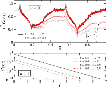
Figure 2: Upper panel: connected density-density correlation function $G(x,t)$ for $X=x/L=1/4$, as a function of the rescaled time $\theta=t/L$, after a quench from the ground state at the critical point $\bar{\mu}_{i}=0$ to $\bar{\mu}_{f}$ such that $\kappa_{f}=\bar{\mu}_{f}L=2$. Continuous curves are for a purely unitary dynamics ($u=0$), where the dynamic FSS (3) is verified; dotted curves are in the presence of incoherent particle losses, with the dissipative coupling $u$ such that $uL^{1.25}=1$. Lower panel: temporal decay of $G(x,t)$ for a dissipative dynamics with $u=1$, at criticality ($\bar{\mu}_{i}=\bar{\mu}_{f}=0$). A much faster decay to an uncorrelated state emerges, with a slope that asymptotically depends only on $x$. All curves are sufficiently accurate to be considered as practically exact, on the scale of this and of all next figures. Here and in the next figures, times are in units of $\hbar/J$.

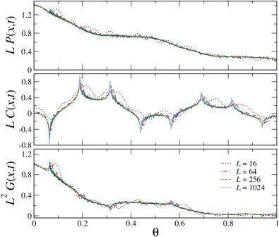
Figure 3: The correlation functions $P(x,t)$ (upper panel), $C(x,t)$ (central panel), and $G(x,t)$ (lower panel), for $X=1/4$, versus $\theta=t/L$. The system has been driven out of equilibrium through a quench from the critical point $\kappa_{i}=0$ to $\kappa_{f}=2$, and by the dissipation induced by incoherent particle losses, for $\gamma=uL=1$. The curves clearly approach a scaling function with increasing $L$, thus supporting the dynamic FSS in Eq. (6) (here and in Fig. 4, data for $L=256$ are hardly distinguishable from those for $L=1024$). Results for other values of $X$, $\kappa_{i,f}$ and $\gamma$ confirm it.

Our protocol starts from the ground state of $\hat{H}_{K}$ for a generic $\bar{\mu}_{i}$, sufficiently small to stay within the critical regime. We then study the time evolution after a quench of the Hamiltonian parameter to $\bar{\mu}_{f}$, and a simultaneous sudden turning on of the dissipation coupling $u$ (see Appendix for details). We consider the fixed-time correlations

$$P(x,t) \!=\! {\rm Tr}[\rho(t)\,(\hat{c}_{j}^{\dagger}\hat{c}_{j+x}^{\dagger}+\hat{c}_{j+x}\hat{c}_{j})],$$ (12a)

$$C(x,t) \!=\! {\rm Tr}[\rho(t)\,(\hat{c}_{j}^{\dagger}\hat{c}_{j+x}+\hat{c}_{j+x}^{\dagger}\hat{c}_{j})],$$ (12b)

$$G(x,t) \!=\! {\rm Tr}[\rho(t)\,\hat{n}_{j}\hat{n}_{j+x}]-{\rm Tr}[\rho(t)\,\hat{n}_{j}]\,{\rm Tr}[\rho(t)\,\hat{n}_{j+x}],\qquad$$ (12c)

where $j,x\in[1,L/2]$ and $\rho(t)$ is the system’s density matrix. The dynamic FSS behavior of the observables (12a)-(12c) is expected to be given by Eq. (6), with $y_{\mu}=1$, $z=1$. Moreover, $\varphi=1$ for the correlations $P$ and $C$ (since the RG dimension of the fermionic operator is $y_{\hat{c}}=y_{\hat{c}^{\dagger}}=1/2$), while $\varphi=2$ for $G$ (since $y_{\hat{n}}=1$). This scaling scenario should hold for all the considered dissipation mechanisms, cf. Eq. (11). Of course, the corresponding scaling functions are expected to differ.

Before analyzing the full model, let us neglect the bath coupling and only consider the unitary dynamics ($u=0$). As is visible from the upper panel of Fig. 2, for density-density correlations $G(x,t)$ (continuous curves), the scaling behavior (3) emerges in the large-$L$ limit after the proper rescaling of the pre- and post-quench control parameter and of time as in Eq. (4). An analogous scenario emerges when $u\ll L^{-z}$; for example for $u\sim L^{-\zeta}$ with $\zeta>z$, the system asymptotically converges to the dynamic FSS scenario with $u=0$ (dotted curves in the upper panel), and thus the coherent dynamics prevails. Conversely, if the coupling $u$ is switched on and kept fixed with $L$, the dissipative dynamics overcomes the critical coherence. Indeed the system exponentially collapses to an uncorrelated state, in a much shorter time scale (bottom panel —the time $t$ has not been rescaled here). The decay rate only depends on the distance $x$, thus no scaling behavior emerges. Similar scenarios appear whenever $u\gg L^{-z}$.

A nontrivial competition between critical coherence and dissipation can be only observed for $u\sim L^{-z}$, cf. Eq. (5), as shown in Fig. 3 for a quench protocol in the presence of incoherent particle losses with rescaled strength $\gamma=uL^{z}=1$. The dynamic FSS prediction (6) is clearly verified. A global check is also provided by the results shown in Fig. 4, for the integrated correlations

$$A_{P}(z,t)=\sum_{x=z}^{L/2}P(x,t),\quad A_{C}(z,t)=\sum_{x=z}^{L/2}C(x,t),$$ (13)

with $0<z<L/2$, which are expected to scale as

$$A_{O}(z,t,\bar{\mu}_{i},\bar{\mu}_{f},u,L)\approx L^{1-2y_{O}}{\cal A}_{O}(Z,\theta,\kappa_{i},\kappa_{f},\gamma)$$ (14)

for $Z\equiv z/L>0$. Note that this definition cannot be extended to $z\to 0$ (more precisely $Z\to 0$), because the integral of the two-point function is singular, in that in the critical continuum limit at equilibrium $C(x)\sim P(x)\sim 1/x$ at small distance Sachdev-book .

Analogous outcomes are obtained for the dissipators related to pumping (not shown) and dephasing (see right panels of Fig. 4). We have validated our picture also for a lattice gas of free nonrelativistic fermions, i.e. $\delta=0$ in Eq. (8), which undergoes a quantum transition lying in a different universality class, with dynamic exponent $z=2$ (not shown).

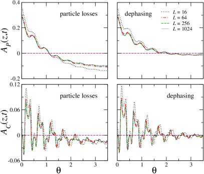
Figure 4: The integrated correlations $A_{P}$ and $A_{C}$, for $Z=z/L=1/4$, versus $\theta=t/L$. The system is quenched from $\kappa_{i}=0$ to $\kappa_{f}=2$, and dissipation is induced either by the presence of incoherent particle losses ($\hat{L}_{{\rm l},j}$, left panels) or by an incoherent dephasing mechanism ($\hat{L}_{{\rm d},j}$, right panels), with $\gamma=1$. The results nicely support Eq. (14), since curves appear to converge to a scaling function with increasing $L$.

IV Conclusions

In summary, our findings confirm the existence of a dynamic regime characterized by the competition between critical coherent and dissipative dynamics, supporting the scaling behaviors put forward within the dynamic FSS framework. We will report elsewhere a more thorough discussion of the numerical results, their convergence rate [which is generally $O(L^{-1})$ in the critical Kitaev model], the particular features of the scaling curves, such as the emerging spikes in the rescaled time $\theta$ (reminiscent of the behavior at dynamical phase transitions Heyl-18 , see Figs. 2 and 3), and the asymptotic behaviors in the large-$\theta$ limit. The dynamic FSS framework can be also used to study other protocols in the presence of dissipation, for example when slowly changing the Hamiltonian parameters across a quantum transition.

The arguments leading to the above scaling scenario are quite general. Analogous phenomena are expected to develop in any homogeneous $d$-dimensional many-body system at a continuous quantum transition, whose Markovian interaction with the bath can be described by local or extended dissipators within a Lindblad equation (1). The regime showing competition of critical coherent and dissipative dynamics is realized when the dissipation parameter $u$ scales as the gap $\Delta$ of the Hamiltonian of the many-body system, i.e.,

$$u\sim\Delta\,.$$ (15)

Since at a quantum transition $\Delta\sim L^{-z}$, this is a low-dissipation regime. This reflects the fact that at a quantum transition the perturbation arising from dissipation is always relevant, such the temperature at equilibrium Sachdev-book ; SGCS-97 ; CPV-14 . Therefore, when $u\gg\Delta$, critical coherent fluctuations do not survive dissipation. These arguments should also apply to non-Markovian system-bath couplings DA-17 (not described by Lindblad equations), replacing $u$ with the parameter controlling the decay rate.

This dynamic scenario has been checked within fermion wires, cf. Eq. (8), in the presence of local dissipation mechanisms associated with the Lindblad operators (11). Further studies would serve to achieve a conclusive validation of our competition theory, for other many-body systems and/or dissipation mechanisms, including nonlocal ones VWC-09 ; DRBZ-11 ; LPK-16 . Further interesting issues may concern quantum thermodynamic properties Thermo-book ; Thermo-book2 ; CF-16 in the competition regime.

Other issues worth being investigated concern the emergence, and characterization, of analogous competition scaling phenomena at first-order quantum transitions, for which dynamic FSS frameworks have been also developed PRV-18 , and new features may arise, like a particular sensitivity on the type of boundary conditions CNPV-14 ; PRV-18c .

We finally mention that some experimental breakthroughs have been recently achieved in the control of dissipative quantum many-body dynamics, through different platforms, such as Rydberg atoms or circuit-QED technology. For example, a quantum critical behavior in such out-of-equilibrium context was reported CRWAW-13 ; TNDTT-17 ; FSLKH-17 . These studies encourage the verification of our competition theory, using a limited (relatively small, say, few tens) amount of controlled objects, which may already suffice to highlight some signatures of dynamic scaling.

Appendix A Solution of Eq. (1) for our Fermi lattice gas model

It is useful to first distinguish between the different schemes of system-bath coupling employed in this work. Specifically, if the dissipation is linear in the creation and/or annihilation operators, as is the case for incoherent particle losses ($\hat{L}_{{\rm l},\,j}=\hat{c}_{j}$) or pumping ($\hat{L}_{{\rm p},\,j}=\hat{c}^{\dagger}_{j}$), the corresponding driven-dissipative quantum dynamics can be exactly solved using an analogous strategy as for standard quadratic Fermi models, which reduces the exponential complexity of the problem to a polynomial one. In contrast, a different method has to be adopted for a dephasing mechanism ($\hat{L}_{{\rm d},\,j}=\hat{n}_{j}$), where, although the full dynamics cannot be simply obtained, it is however possible to track the time evolution of certain expectation values, using a polynomial amount of resources.

In this respect, this appendix contains an excerpt of some technicalities which have been already detailed in Refs. Prosen-08 ; HC-13 ; KMSFR-17 . These are reported here for the sake of clarity, and in order to make our discussion self consistent and useful to anyone who needs to reproduce our results. On top of that, we also provide additional details on the specific observables discussed in Sec. III, and on the implementation of the antiperiodic boundary conditions for our model.

A.1 Quantum dynamics in the presence of incoherent losses or pumping

For $\hat{L}_{j}=\hat{c}^{(\dagger)}_{j}$, the dissipator ${\mathbb{D}}[\rho]=\sum_{o}{\mathbb{D}}_{o}[\rho]$ in Eq. (1) turns out to be quadratic in the fermionic creation and annihilation operators (notice that the index $o$ here corresponds to a lattice site, denoted by $j$). The same feature holds for the Kitaev Hamiltonian in Eq. (8). As a consequence and since the system is translationally invariant, it is useful to perform a Fourier transformation applied to creation/annihilation operators for fermions on the chain Sachdev-book :

$$\hat{c}_{j}=\frac{e^{-i\pi/4}}{\sqrt{L}}\sum_{k}\hat{c}_{k}e^{ikj},\qquad(j=1,\ldots,L).$$ (16)

This transformation preserves the fermionic anticommutation rules, that is,

$$\{\hat{c}_{j},\hat{c}_{l}\}\!=\!0,\;\; \{\hat{c}_{j}^{\dagger},\hat{c}_{l}\}\!=\!\delta_{j,l},$$ real space, (17a)

$$\{\hat{c}_{k},\hat{c}_{q}\}\!=\!0,\;\; \{\hat{c}_{k}^{\dagger},\hat{c}_{q}\}\!=\!\delta_{k,q},$$ momentum space. (17b)

Considering, without loss of generality, an even number $L$ of sites in the chain, antiperiodic boundary conditions can be enforced by choosing the following set of momenta:

$$k=\Big{\{}\pm\frac{\pi}{L}(2n+1)\Big{\}},\quad n=0,1,\cdots,L/2-1.$$ (18)

Indeed, adopting such choice and using the definition in Eq. (16), it is easy to see that

$$\hat{c}^{(\dagger)}_{j+L}=-\hat{c}^{(\dagger)}_{j},\qquad\forall j\in[1,L].$$ (19)

The density operator $\rho(t)$ at time $t=0$ is taken as the ground state of $\hat{H}_{\rm K}$. This can be cast in a tensor product form, after going in momentum space:

$$\rho(0)=\bigotimes_{k>0}\rho_{k}(0).$$ (20)

Here $\rho_{k}(0)$ denotes the restricted density operator describing the configuration of the $k$-sector (with $k>0$), that is, the sector containing contributions associated to excitations having momentum $\pm|k|$. Due to the structure of the Lindblad master equation, $\rho(t)$ is factorized in momentum space for any time $t$. As a consequence, the behavior in each $k$-sector can be determined by solving a differential system having the following structure (in units of $\hslash=1$):

$$\frac{d}{dt}\rho_{k}(t)=-i\big{[}\hat{H}_{k},\rho_{k}(t)\big{]}+u\,\mathbb{D}[\rho_{k}],\quad k>0.$$ (21)

The Hamiltonian

$$\hat{H}_{k}=\left(\begin{matrix}0&0&0&2\,|\!\sin k|\\ 0&-2f_{k}(\mu)&0&0\\ 0&0&-2f_{k}(\mu)&0\\ 2\,|\!\sin k|&0&0&-4f_{k}(\mu)\end{matrix}\right),$$ (22)

with $f_{k}(\mu)=\mu/2+\cos k$ [we put $J=\delta=1$ in Eq. (8)], governs the dynamics in the four dimensional state basis $\{|0_{k}\rangle,\,|1_{k}\rangle,\,|1_{-k}\rangle,\,|1_{k},\,1_{-k}\rangle\}$. The dissipator in the corresponding $k$-sector violates the fermion parity; for the case of homogeneous particle losses (i.e., $\hat{L}_{j}=\hat{c}_{j}$) this is given by

$$\mathbb{D}[\rho_{k}] = \hat{c}_{k}\rho_{k}\hat{c}^{\dagger}_{k}-\tfrac{1}{2}(\hat{n}_{k}\rho_{k}+\rho_{k}\hat{n}_{k})+$$ (23)

$$+ \hat{c}_{-k}\rho_{k}\hat{c}^{\dagger}_{-k}-\tfrac{1}{2}(\hat{n}_{-k}\rho_{k}+\rho_{k}\hat{n}_{-k}).$$

A very similar expression for $\mathbb{D}[\rho_{k}]$ holds, with analogous properties as those for Eq. (23), in the case of homogeneous particle pumping (i.e., $\hat{L}_{j}=\hat{c}^{\dagger}_{j}$), provided these substitutions are applied in the above equation:

$$\hat{c}_{k}\to\hat{c}^{\dagger}_{k}, \hat{c}_{-k}\to\hat{c}^{\dagger}_{-k},$$ (24a)

$$\hat{c}^{\dagger}_{k}\to\hat{c}_{k}, \hat{c}^{\dagger}_{-k}\to\hat{c}_{-k},$$ (24b)

$$\hat{n}_{k}\to\hat{c}_{k}\hat{c}^{\dagger}_{k}, \hat{n}_{-k}\to\hat{c}_{-k}\hat{c}^{\dagger}_{-k}.$$ (24c)

Once the structure of all the $\rho_{k}(t)$ matrices is determined by explicitly solving Eq. (21) in the corresponding four-dimensional Hilbert $k$-subspace (recall that $k>0$), the time evolution of any observable can be computed simply by inverting the mapping in Eq. 16. Indeed, given an observable $\hat{\mathcal{O}}(\{\hat{c}_{j}\},\{\hat{c}_{j}^{\dagger}\})$ in real space, its explicit time evolution is obtained by moving into momentum space: $\hat{\mathcal{O}}(\{\hat{c}_{k}\},\{\hat{c}^{\dagger}_{k}\})$ and then considering the average

$$\langle\hat{\mathcal{O}}\rangle(t)=\mbox{Tr}\Big{[}\hat{\mathcal{O}}\big{(}\{\hat{c}_{k}\},\{\hat{c}^{\dagger}_{k}\}\big{)}\,\bigotimes_{k>0}\rho_{k}(t)\Big{]}.$$ (25)

In the present case, we also have that

$$\langle\hat{c}_{k}\rangle(t)=\langle\hat{c}^{\dagger}_{k}\rangle(t)=0,\quad\forall t,\,k\,.$$ (26)

This can be easily shown by considering the equations of motion for such amplitudes. As a consequence, the only operators that can have non-zero expectation value are those corresponding to products of an even number of fermionic operators in each $k$-subspace. In all the other cases, the expectation values are zero, due to Eq. 26 and to the anticommutation rules (17).

Let us now explicitly consider the pairing correlation function $P(x,t)$ [see Eq. (12a)], that is,

$$P(x,t)=\langle\hat{c}^{\dagger}_{j}\hat{c}^{\dagger}_{j+x}\rangle(t)+\langle\hat{c}_{j+x}\hat{c}_{j}\rangle(t).$$ (27)

Such quantity in momentum space is given by

$$P(x,t)=\bigg{[}\frac{e^{i\pi/2}}{L}\!\!\sum_{k,q}e^{-i[kj+q(j+x)]}\langle\hat{c}^{\dagger}_{k}\hat{c}^{\dagger}_{q}\rangle(t)\bigg{]}+{\rm h.c.}$$ (28)

Due to the constraint listed above, we also have that

$$\langle\hat{c}_{k}\hat{c}_{q}\rangle(t)\neq 0\quad\Longleftrightarrow\quad k=-q.$$ (29)

As a consequence, the expression in Eq. (28) further simplifies into

$$P(x,t)=\bigg{[}\frac{e^{i\pi/2}}{L}\sum_{k}e^{ikx}\langle\hat{c}^{\dagger}_{k}\hat{c}^{\dagger}_{-k}\rangle(t)\bigg{]}+{\rm h.c.},$$ (30)

which can be eventually written in a more compact form as

$$P(x,t)=-\frac{2}{L}\sum_{k>0}\sin(kx)\left[\langle c^{\dagger}_{k}c^{\dagger}_{-k}\rangle(t)+{\rm h.c.}\right].$$ (31)

By exploiting the same strategy, it is possible to decompose any mean value as a combination of amplitudes that involve expectation values in momentum space. For instance, if one considers the correlation function $C(x,t)$ of Eq. (12b), one finds the expression

$$C(x,t)=\frac{2}{L}\sum_{k>0}\cos(kx)\left[\langle\hat{c}^{\dagger}_{k}\hat{c}_{k}\rangle(t)+\langle\hat{c}^{\dagger}_{-k}\hat{c}_{-k}\rangle(t)\right].$$ (32)

As the number of operators in real space increases, the structure in momentum space becomes more cumbersome. This is the case for the four-point connected density-density operator $G(x,t)$ of Eq. (12c), which can be expressed as

$$G(x,t)=\frac{\delta_{x,0}}{L}\sum_{k>0}\left[\langle\hat{n}_{k}\rangle+\langle\hat{n}_{-k}\rangle\right]+\frac{2}{L^{2}}\sum_{k>0}\Big{\{}\big{[}\cos(2kx)-1\big{]}\big{[}\langle\hat{n}_{k}\rangle\langle\hat{n}_{-k}\rangle-\langle\hat{n}_{k}\hat{n}_{-k}\rangle+\langle\hat{c}^{\dagger}_{k}\hat{c}^{\dagger}_{-k}\rangle\langle\hat{c}_{-k}\hat{c}_{k}\rangle\big{]}\Big{\}}$$

$$+\frac{4}{L^{2}}\bigg{\{}\!\sum_{k>0}\sin(kx)\langle\hat{c}^{\dagger}_{k}\hat{c}^{\dagger}_{-k}\rangle\!\bigg{\}}\bigg{\{}\!\sum_{k>0}\sin(kx)\langle\hat{c}_{-k}\hat{c}_{k}\rangle\!\bigg{\}}\!-\!\frac{1}{L^{2}}\bigg{\{}\!\sum_{k>0}\left[e^{ikx}\langle\hat{n}_{k}\rangle+e^{-ikx}\langle\hat{n}_{-k}\rangle\right]\!\bigg{\}}\bigg{\{}\!\sum_{k>0}\left[e^{-ikx}\langle\hat{n}_{k}\rangle+e^{ikx}\langle\hat{n}_{-k}\rangle\right]\!\bigg{\}},$$ (33)

where, for the ease of compactness, we have omitted the time dependence of all the expectation values.

We end up by mentioning that antiperiodic boundary conditions are automatically guaranteed by adopting the choice of momenta $k$ written in Eq. (18). The expressions we have reported for the correlations in $k$-space correspond to measuring them in real space within the chain length, that is, by taking $j,x\in[1,L/2]$ in Eq. (27) (and similar). Otherwise, a minus sign would appear each time the boundary is crossed an odd number of times, since

$$\hat{c}^{(\dagger)}_{j+mL}=(-1)^{m}\hat{c}^{(\dagger)}_{j},\quad\forall j\in[1,L].$$ (34)

Notice also that the following symmetries always hold (where $x\in[1,L]$), due to antiperiodic boundaries:

$$P(x,t) = P(L-x,t),$$ (35a)

$$C(x,t) = -C(L-x,t),$$ (35b)

$$G(x,t) = G(L-x,t).$$ (35c)

A.2 Quantum dynamics in the presence of dephasing

Unfortunately, the quantum dynamics of the fermionic Kitaev chain in the presence of dephasing Lindblad terms $\hat{L}_{{\rm d},j}=\hat{n}_{j}=\hat{c}^{\dagger}_{j}\hat{c}_{j}$ does not factorize in momentum space, since the dissipator ${\mathbb{D}}[\rho]$ now becomes quartic in the creation/annihilation operators. As a consequence, the method described in App. A.1 cannot be exploited and, in general, an exact solution in terms of a polynomial scaling with $L$ cannot be obtained. Nonetheless, one could pay attention only to the time evolution of certain observables of interest. We recall that, in order to determine the behavior of a given time-dependent expectation value $\langle\hat{\mathcal{O}}\rangle(t)$, one needs to solve the following differential equation BP-book

$$\frac{d}{dt}\hat{\mathcal{O}}=i\big{[}\hat{H},\hat{\mathcal{O}}\big{]}+u\,\tilde{\mathbb{D}}[\hat{\mathcal{O}}],$$ (36)

where

$$\tilde{\mathbb{D}}[\hat{\mathcal{O}}]=\sum_{j}\left[\hat{L}^{\dagger}_{j}\hat{\mathcal{O}}\hat{L}_{j}-\tfrac{1}{2}\big{\{}\hat{L}^{\dagger}_{j}\hat{L}_{j},\hat{\mathcal{O}}\big{\}}\right]$$ (37)

denotes the dissipator in the Heisenberg picture.

Solving Eq. (36) for a many-body system is generally an hard task, unless explicit constructions as the one reported in App. A.1 are possible. Indeed, the time evolution of a given operator usually depends also on that of other observables. As a consequence, solving a single equation of motion actually requires to deal with a number of differential equations that usually grows exponentially with the system size $L$.

In the present case, for the two-point observables $P(x,t)$ and $C(x,t)$ of Eqs. (12a) and (12b), it is however possible to find a closed set of equations of motion, whose dimension grows only polynomially with increasing $L$. Such set is given by all the quadratic observables in the fermionic operators. In such case, the time evolution of any two point amplitude [as is the case for $P(x,t)$ and $C(x,t)$], can be rephrased in terms of the behavior of the following 4$L$ amplitudes:

$$\langle\mathcal{\hat{A}}_{x}\rangle(t) \equiv \langle\hat{c}_{j}\hat{c}_{j+x}\rangle(t),$$ (38a)

$$\langle\mathcal{\hat{B}}_{x}\rangle(t) \equiv \langle\hat{c}_{j}\hat{c}^{\dagger}_{j+x}\rangle(t),$$ (38b)

$$\langle\mathcal{\hat{C}}_{x}\rangle(t) \equiv \langle\hat{c}^{\dagger}_{j}\hat{c}_{j+x}\rangle(t),$$ (38c)

$$\langle\mathcal{\hat{D}}_{x}\rangle(t) \equiv \langle\hat{c}^{\dagger}_{j}\hat{c}^{\dagger}_{j+x}\rangle(t).$$ (38d)

Here we always suppose that $j\in[1,L]$ and $j+x\in[1,L]$, such that the boundaries of the chain are never crossed. By plugging these operators in Eq. (36), one arrives at the following set of $4L$ coupled differential equations governing the time evolution of the corresponding amplitudes in Eqs. (38):

$$\frac{d\mathcal{\hat{A}}_{x}}{dt} = 2i(\mathcal{\hat{A}}_{x-1}+\mathcal{\hat{A}}_{x+1})+i(\mathcal{\hat{C}}_{x-1}-\mathcal{\hat{C}}_{x+1})-i(\mathcal{\hat{B}}_{x-1}-\mathcal{\hat{B}}_{x+1})+2i\mu\mathcal{\hat{A}}_{x}-u\,\mathcal{\hat{A}}_{x},$$ (39a)

$$\frac{d\mathcal{\hat{B}}_{x}}{dt} = i(\mathcal{\hat{D}}_{x-1}-\mathcal{\hat{D}}_{x+1})+i(\mathcal{\hat{A}}_{x-1}-\mathcal{\hat{A}}_{x+1})-u\,\mathcal{\hat{B}}_{x}(1-\delta_{x,0}),$$ (39b)

$$\frac{d\mathcal{\hat{C}}_{x}}{dt} = -i(\mathcal{\hat{D}}_{x-1}-\mathcal{\hat{D}}_{x+1})-i(\mathcal{\hat{A}}_{x-1}-\mathcal{\hat{A}}_{x+1})-u\,\mathcal{\hat{C}}_{x}(1-\delta_{x,0}),$$ (39c)

$$\frac{d\mathcal{\hat{D}}_{x}}{dt} = -2i(\mathcal{\hat{D}}_{x-1}+\mathcal{\hat{D}}_{x+1})+i(\mathcal{\hat{C}}_{x-1}-\mathcal{\hat{C}}_{x+1})-i(\mathcal{\hat{B}}_{x-1}-\mathcal{\hat{B}}_{x+1})-2i\mu\mathcal{\hat{D}}_{x}-u\,\mathcal{\hat{D}}_{x}.$$ (39d)

Since one is looking for the structure of four different kinds of amplitudes and $x$ can take values from $0$ to $L-1$, the number of coupled equations is $4L$. Indeed, due to the presence of first-neighbor coupling terms in the Kitaev chain, the amplitudes corresponding to operators at distance $x$ are related to those at distance $x+1$ and $x-1$. However, due to translational invariance and fermionic statistics, such amplitudes possess symmetry properties that enable to reduce the amount of coupled equations of motion to be solved. Indeed the following relations hold ($x\in[0,L-1]$):

$$\mathcal{\hat{A}}_{x} = -\mathcal{\hat{A}}_{-x},$$ (40a)

$$\mathcal{\hat{B}}_{x} = -\mathcal{\hat{C}}_{-x}+\delta_{x,0},$$ (40b)

$$\mathcal{\hat{D}}_{x} = -\mathcal{\hat{D}}_{-x}.$$ (40c)

In addition, by exploiting antiperiodic boundary conditions, we have that ($y\in[0,L/2-1]$):

$$\mathcal{\hat{A}}_{L/2+y}=\hat{c}_{L/2}\hat{c}_{L+y}=-\hat{c}_{L/2}\hat{c}_{y}=\hat{c}_{y}\hat{c}_{L/2}=\mathcal{\hat{A}}_{L/2-y},$$

$$\mathcal{\hat{B}}_{L/2+y}=\hat{c}_{L/2}\hat{c}^{\dagger}_{L+y}=-\hat{c}_{L/2}\hat{c}^{\dagger}_{y}=\hat{c}^{\dagger}_{y}\hat{c}_{L/2}=\mathcal{\hat{C}}_{L/2-y},$$

$$\mathcal{\hat{C}}_{L/2+y}=\hat{c}^{\dagger}_{L/2}\hat{c}_{L+y}=-\hat{c}^{\dagger}_{L/2}\hat{c}_{y}=\hat{c}_{y}\hat{c}^{\dagger}_{L/2}=\mathcal{\hat{B}}_{L/2-y},$$

$$\mathcal{\hat{D}}_{L/2+y}=\hat{c}^{\dagger}_{L/2}\hat{c}^{\dagger}_{L+y}=-\hat{c}^{\dagger}_{L/2}\hat{c}^{\dagger}_{y}=\hat{c}^{\dagger}_{y}\hat{c}^{\dagger}_{L/2}=\mathcal{\hat{D}}_{L/2-y},$$ (41)

where we have plugged $j=L/2$ in Eqs. (38). It is thus clear that the full problem for the above two-point correlators is actually $(2L+2)$-dimensional, since it is sufficient to write the corresponding coupled equations for the operators: $\mathcal{\hat{A}}_{x\in[1,L/2]}$, $\mathcal{\hat{B}}_{x\in[0,L/2]}$, $\mathcal{\hat{C}}_{x\in[0,L/2]}$, $\mathcal{\hat{D}}_{x\in[1,L/2]}$. Notice also that one trivially has $\mathcal{\hat{A}}_{0}=\mathcal{\hat{D}}_{0}=0$.

The initial conditions for the differential system (39) correspond to the expectation values of such operators evaluated on the ground state of the Kitaev chain for a given value of the control parameter $\mu=\mu_{i}$, and can be immediately found by means of a Bogoliubov transformation in real space, which generalizes the standard procedure in $k$-space to nonhomogeneous quadratic systems. Once the time evolution of the amplitudes (38) is determined, the behavior of the two-point observables $P(x,t)$ and $C(x,t)$ for $x\in[1,L/2]$ can be easily accessed by noticing that

$$P(x,t) = \langle\mathcal{\hat{D}}_{x}\rangle(t)-\langle\mathcal{\hat{A}}_{x}\rangle(t)=2\,{\rm Re}\big{[}\langle\mathcal{\hat{D}}_{x}\rangle(t)\big{]},\qquad$$ (42a)

$$C(x,t) = \langle\mathcal{\hat{C}}_{x}\rangle(t)-\langle\mathcal{\hat{B}}_{x}\rangle(t).$$ (42b)

References

- (1) A. A. Houck, H. E. Türeci, and J. Koch, On-chip quantum simulation with superconducting circuits, Nat. Phys. 8, 292 (2012).
- (2) M. Müller, S. Diehl, G. Pupillo, and P. Zoller, Engineered open systems and quantum simulations with atoms and ions, Adv. At. Mol. Opt. Phys. 61, 1 (2012).
- (3) I. Carusotto and C. Ciuti, Quantum fluids of light, Rev. Mod. Phys. 85, 299 (2013).
- (4) M. Aspelmeyer, T. J. Kippenberg, and F. Marquardt, Cavity optomechanics, Rev. Mod. Phys. 86, 1391 (2014).
- (5) S. Sachdev, Quantum Phase Transitions, (Cambridge University, Cambridge, England, 1999).
- (6) H.-P. Breuer and F. Petruccione, The Theory of Open Quantum Systems (Oxford University Press, New York, 2002).
- (7) A. Rivas and S. F. Huelga, Open Quantum System: An Introduction (SpringerBriefs in Physics, Springer, 2012).
- (8) A. Yu. Kitaev, Unpaired Majorana fermions in quantum wires, Phys. Usp. 44, 131 (2001).
- (9) S. L. Sondhi, S. M. Girvin, J. P. Carini, and D. Shahar, Continuous quantum phase transitions, Rev. Mod. Phys. 69, 315 (1997).
- (10) G. Lindblad, On the generators of quantum dynamical semigroups, Commun. Math. Phys. 48, 119 (1976).
- (11) V. Gorini, A. Kossakowski, and E. C. G. Sudarshan, Completely positive dynamical semigroups of N-level systems, J. Math. Phys. 17, 821 (1976).
- (12) L. M. Sieberer, M. Buchhold, and S. Diehl, Keldysh field theory for driven open quantum systems, Rep. Prog. Phys. 79, 096001 (2016).
- (13) M. Campostrini, A. Pelissetto, and E. Vicari, Finite-size scaling at quantum transitions, Phys. Rev. B 89, 094516 (2014).
- (14) M. Campostrini, J. Nespolo, A. Pelissetto, and E. Vicari, Finite-size scaling at first-order quantum transitions, Phys. Rev. Lett. 113, 070402 (2014).
- (15) A. Pelissetto, D. Rossini, and E. Vicari, Dynamic finite-size scaling after a quench at quantum transitions, Phys. Rev. E 97, 052148 (2018).
- (16) D. Nigro, D. Rossini, and E. Vicari, Scaling properties of work fluctuations after quenches near quantum transitions, J. Stat. Mech. (2019) 023104.
- (17) S. Yin, P. Mai, and F. Zhong, Nonequilibrium quantum criticality in open systems: The dissipation rate as an additional indispensable scaling variable, Phys. Rev. B 89, 094108 (2014); S. Yin, C.-Y. Lo, and P. Chen, Scaling behavior of quantum critical relaxation dynamics of a system in a heat bath, Phys. Rev. B 93, 184301 (2016).
- (18) D. Rossini and E. Vicari, Scaling behavior of the stationary states arising from dissipation at continuous quantum transitions, arXiv:1907.02631 (2019) [Phys. Rev. B, to be published].
- (19) Note however that the non-local Jordan-Wigner transformation of the Ising chain with periodic or antiperiodic boundary conditions does not map into the fermionic model (8) with periodic or antiperiodic boundary conditions. Indeed further considerations apply Katsura-62 ; Pfeuty-70 , leading to a less straightforward correspondence, depending on the parity of the particle number eigenvalue. Therefore, although their bulk behaviors in the infinite-volume limit, and thus their phase diagram, are analogous, the resulting FSS functions differ, since they depend on the choice of the boundary conditions.
- (20) S. Katsura, Statistical mechanics of the anisotropic linear Heisenberg model, Phys. Rev. 127, 1508 (1962).
- (21) P. Pfeuty, The one-dimensional Ising model with a transverse field, Ann. Phys. 57, 79 (1970).
- (22) B. Horstmann, J. I. Cirac, and G. Giedke, Noise-driven dynamics and phase transitions in fermionic systems, Phys.Rev. A 87, 012108 (2013).
- (23) M. Keck, S. Montangero, G. E. Santoro, R. Fazio, and D. Rossini, Dissipation in adiabatic quantum computers: lessons from an exactly solvable model, New. J. Phys. 19, 113029 (2017).
- (24) T. Prosen, Third quantization: a general method to solve master equations for quadratic open Fermi systems, New J. Phys. 10, 043026 (2008).
- (25) V. Eisler, Crossover between ballistic and diffusive transport: the quantum exclusion process, J. Stat. Mech. (2011) P06007.
- (26) E. B. Davies, Quantum stochastic processes II, Commun. Math. Phys. 19, 83 (1970); Quantum stochastic processes, Commun. Math. Phys. 15, 277 (1969).
- (27) D. E. Evans, Irreducible Quantum Dynamical Semigroups, Commun. math. Phys. 54, 293 (1977).
- (28) S. G. Schirmer and X. Wang, Stabilizing open quantum systems by Markovian reservoir engineering, Phys. Rev. A 81, 062306 (2010).
- (29) D. Nigro, On the uniqueness of the steady-state solution of the Lindblad-Gorini-Kossakowski-Sudarshan equation, J. Stat. Mech. (2019) 043202.
- (30) M. Heyl, Dynamical quantum phase transitions: a review, Rep. Prog. Phys. 81, 054001 (2018).
- (31) I. de Vega and D. Alonso, Dynamics of non-Markovian open quantum systems, Rev. Mod. Phys. 89, 015001 (2017).
- (32) F. Verstraete, M. Wolf, and J. I. Cirac, Quantum computation and quantum-state engineering driven by dissipation, Nat. Phys. 5, 633 (2009).
- (33) S. Diehl, E. Rico, M. A. Baranov, and P. Zoller, Topology by dissipation in atomic quantum wires, Nat. Phys. 7, 971 (2011).
- (34) A. C. Y. Li, F. Petruccione, and J. Koch, Resummation for nonequilibrium perturbation theory and application to open quantum lattices, Phys. Rev. X 6, 021037 (2016).
- (35) Thermodynamics in the quantum regime: Fundamental aspects and new directions, F. Binder, L. A. Correa, C. Gogolin, J. Anders, and G. Adesso (Eds.) (Springer International Publishing, 2018).
- (36) S. Deffner and S. Campbell, Quantum Thermodynamics: An introduction to the thermodynamics of quantum information (Morgan & Claypool Publishers, San Rafael, CA, 2019).
- (37) M. Campisi and R. Fazio, The power of a critical heat engine, Nat. Commun. 7, 11895 (2016).
- (38) A. Pelissetto, D. Rossini, and E. Vicari, Finite-size scaling at first-order quantum transitions when boundary conditions favor one of the two phases, Phys. Rev. E 98, 032124 (2018).
- (39) C. Carr, R. Ritter, C. G. Wade, C. S. Adams, and K. J. Weatherill, Nonequilibrium phase transition in a dilute Rydberg ensemble, Phys. Rev. Lett. 111, 113901 (2013).
- (40) T. Tomita, S. Nakajima, I. Danshita, Y. Takasu, and Y. Takahashi, Observation of the Mott insulator to superfluid crossover of a driven-dissipative Bose-Hubbard system, Sci. Adv. 3, e1701513 (2017).
- (41) M. Fitzpatrick, N. M. Sundaresan, A. C. Y. Li, J. Koch, and A. A. Houck, Observation of a Dissipative Phase Transition in a One-Dimensional Circuit QED Lattice, Phys. Rev. X 7, 011016 (2017).