Self-excited oscillation and synchronization of an on-fiber optomechanical cavity

Abstract

We study a fully on-fiber optomechanical cavity and characterize its performance as a sensor. The cavity is formed by patterning a suspended metallic mirror near the tip of an optical fiber and by introducing a static reflector inside the fiber. Optically induced self-excited oscillation (SEO) is observed above a threshold value of the injected laser power. The SEO phase can be synchronized by periodically modulating the optical power that is injected into the cavity. Noise properties of the system in the region of synchronization are investigated. Moreover, the spectrum is measured near different values of the modulation frequency, at which phase locking occurs. A universal behavior is revealed in the transition between the regions of phase locked and free running SEO.

I Introduction

Resonant detection is a widely employed technique in a variety of applications. A detector belonging to this class typically consists of a resonator, which is characterized by an angular resonance frequency $\omega_{0}$ and characteristic damping rate $\gamma_{0}$. Detection is achieved by coupling a physical parameter of interest, denoted here as $q$, to the resonator in such a way that $\omega_{0}$ becomes $q$ dependent. The sensitivity of the detection scheme that is employed for monitoring the parameter of interest $q$ can be characterized by the minimum detectable change in $q$, denoted as $\delta_{q}$. For small changes, $\delta_{q}$ is related to the minimum detectable relative change in the frequency $\sigma_{\mathrm{\omega}}=\delta_{\omega_{0}}/\omega_{0}$ by the relation $\delta_{q}=\left|\partial\omega_{0}/\partial q\right|^{-1}\omega_{0}\sigma_{\mathrm{\omega}}$. The dimensionless parameter $\sigma_{\mathrm{\omega}}$, in turn, typically depends on the noises affecting the resonator and on the averaging time $t_{\mathrm{a}}$ of the measurement.

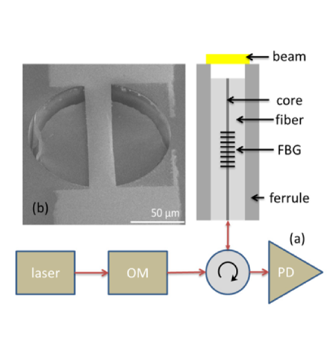
Figure 1: Experimental setup. (a) A schematic drawing of the sample and the experimental setup. An on-fiber optomechanical cavity is excited by a tunable laser with external optical modulator (OM). The mechanical resonator has quality factor $\omega_{0}/2\gamma_{0}=3800$ and the cavity has finesse $\beta_{\mathrm{F}}=2.1$. The reflected light intensity is measured using a photodetector (PD), which is connected to both a spectrum analyzer and an oscilloscope (not shown in the sketch). (b) Electron micrograph of the suspended micromechanical mirror, whose mass is $m=1.1\times 10^{-12}\operatorname{kg}$.

A commonly employed detection scheme is based on externally driving the resonator with a monochromatic force at a frequency close to the resonance frequency and monitoring the response using homodyne detection. For this case the normalized minimum detectable change in the frequency is found to be given by $\sigma_{\mathrm{\omega}}=\sigma_{\mathrm{{\omega}0}}$, where Cleland_2758

$$\sigma_{\mathrm{{\omega}0}}=\left(\frac{2\gamma_{0}k_{\mathrm{B}}T_{\mathrm{eff}}}{U_{0}\omega_{0}^{2}t_{\mathrm{a}}}\right)^{1/2}\ ,$$ (1)

$k_{\mathrm{B}}$ is the Boltzmann’s constant, $T_{\mathrm{eff}}$ is the noise effective temperature and $U_{0}$ is the energy stored in the externally driven resonator in steady state. Note that Eq. (1) is derived by assuming that the response of the resonator is linear and by assuming the classical limit, i.e. $k_{\mathrm{B}}T_{\mathrm{eff}}\gg\hbar\omega_{0}$, where $\hbar$ is Planks’s constant. The generalization of Eq. (1) for the case of nonlinear response is discussed in Ref. Buks_026217 . Note that other contributions to $\sigma_{\mathrm{\omega}}$ (e.g. instrumental noise) are not analyzed in this paper.

In the just mentioned scheme the resonator is driven into a so-called state of forced oscillation (FO) by applying a fixed periodic external force. Alternatively, in some cases back-reaction effects can be exploited for generating a so-called state of self-excited oscillation (SEO) Rugar1989 ; Arcizet2006a ; Forstner2012 ; Weig2013 . In this paper we study SEO in an on-fiber optomechanical cavity device (see Fig. 1), which is formed between a fiber Bragg grating (FBG) mirror, serving as a static reflector, and a vibrating mirror fabricated on a mechanical resonator next to the tip of the single mode optical fiber. The movable mirror can be driven into the SEO state by injecting a monochromatic laser light into the fiber. The SEO occurs via bolometric feedback effects. Further, by periodically modulating the laser intensity it is possible to lock the phase of SEO to a rational fraction of the modulation frequency.

Driving an on-fiber optomechanical cavity into the state of SEO is easier in comparison with the case of FO, which requires the fabrication of additional elements near the tip of the fiber that need to be electrically wired. In contrast, SEO can be induced by optical excitation only. In this paper, we study the performance of the device as a sensor in the regime of SEO, both with and without synchronization, and compare the results to the case of FO [see Eq. (1)]. We find that synchronization gives rise to a suppression in phase noise, which in turn allows a sensitivity enhancement.

Optomechanical cavities Braginsky_653 ; Hane_179 ; Gigan_67 ; Metzger_1002 ; Kippenberg_1172 ; Favero_104101 ; Marquardt2009 are widely employed for various sensing Rugar1989 ; Arcizet2006a ; Forstner2012 ; Weig2013 and photonics Lyshevski&Lyshevski_03 ; Stokes_et_al_90 ; Hossein_Zadeh_276 ; Wu_et_al_06 ; MattEichenfield2007 ; Bahl2011 ; FlowersJacobs_221109 applications. Such systems may allow experimental study of the crossover between classical to quantum realms Poot_273 . The effect of radiation pressure typically governs the optomechanical coupling (i.e. the coupling between the electromagnetic cavity and the mechanical resonator that serves as a movable mirror) when the finesse of the optical cavity is sufficiently high Kippenberg_et_al_05 ; Rokhsari2005 ; Arcizet2006 ; Gigan_67 ; Cooling_Kleckner06 ; Kippenberg_1172 , whereas, bolometric effects can contribute to the optomechanical coupling when optical absorption by the vibrating mirror is significant Metzger_1002 ; Jourdan_et_al_08 ; Marino&Marin2011PRE ; Metzger_133903 ; Restrepo_860 ; Liberato_et_al_10 ; Marquardt_103901 ; Paternostro_et_al_06 ; Yuvaraj_430 . Generally, bolometric effects are dominant in systems comprising of relatively large mirrors, in which the thermal relaxation rate is comparable to the mechanical resonance frequency Aubin_1018 ; Marquardt_103901 ; Paternostro_et_al_06 ; Liberato_et_al_10_PRA . These systems Metzger_133903 ; Metzger_1002 ; Aubin_1018 ; Jourdan_et_al_08 ; Zaitsev_046605 ; Zaitsev_1589 exhibit many intriguing phenomena including mode cooling Hane_179 ; Kim_1454225 ; Aubin_1018 ; Carmon_223902 ; Marquardt_103901 ; Corbitt_021802 ; Carmon_123901 ; Metzger_133903 and synchronization Shlomi_032910 ; Wang_023007 .

II Experimental setup

The optomechanical cavity, which is schematically shown in Fig. 1(a), was fabricated on the flat polished tip of a single mode fused silica optical fiber with outer diameter of $126\operatorname{\mu m}$ (Corning SMF-28 operating at wavelength band around $1550\operatorname{nm}$) held in a zirconia ferrule Yuvaraj_210403 . A $10\operatorname{nm}$ thick chromium layer and a $200\operatorname{nm}$ gold layer were successively deposited by thermal evaporation. The bilayer was directly patterned by a focused ion beam to the desired mirror shape ($20\operatorname{\mu m}$ wide doubly clamped beam). Finally, the mirror was released by etching approximately $12\operatorname{\mu m}$ of the underlying silica in 7% HF acid ($90\operatorname{min}$ etch time at room temperature). The suspended mirror remained supported by the zirconia ferrule, which is resistant to HF.

The static mirror of the optomechanical cavity was provided by a FBG mirror Zaitsev_046605 (made using a standard phase mask technique Anderson_566 , with grating period of $0.527\operatorname{\mu m}$ and length $\approx 8\operatorname{mm}$) having reflectivity band of $0.4\operatorname{nm}$ full width at half maximum centered at $\lambda_{0}=1545\operatorname{nm}$. The length of the optical cavity was $l\approx 10\operatorname{mm}$, providing a free spectral range of $\Delta\lambda=\lambda_{0}^{2}/2n_{\mathrm{eff}}l\approx 80$ pm (where $n_{\mathrm{eff}}$ $=1.468$ is the effective refraction index for SMF-28).

Monochromatic light was injected into the fiber bearing the cavity on its tip from a laser source with an adjustable output wavelength $\lambda$ and power level $P_{\mathrm{L}}$. The laser was connected through an optical circulator, that allowed the measurement of the reflected light intensity $P_{\mathrm{R}}$ by a fast responding photodetector [see Fig. 1(a)]. The detected signal was analyzed by an oscilloscope and a spectrum analyzer. The experiments were performed in vacuum (at residual pressure below $0.01\operatorname{Pa}$) at a base temperature of $77\operatorname{K}$.

The optically-induced SEO in our device is attributed to the bolometric optomechanical coupling between the optical mode and the mechanical resonator Zaitsev_046605 ; Zaitsev_1589 . While the phase of SEO randomly diffuses in time when the laser power that is injected into the cavity is kept constant, phase locking Anishchenko_117 ; Pandey_3 ; Paciorek_1723 ; Adler_351 ; Jensen_1637 ; DosSantos_1147 may occur when the laser power is periodically modulated in time. Such locking results in entrainment Hamerly_1504_04410 , i.e. synchronization huygens1986pendulum ; Rosenblum_401 between the SEO and the external modulation Georg_043603 .

III Evolution equation

In the limit of small displacement the dynamics of the system can be approximately described using a first order evolution equation given by Zaitsev_1589 ; Dykman_1646

$$\dot{A}+\left(\Gamma_{\mathrm{eff}}+i\Omega_{\mathrm{eff}}\right)A=\xi\left(t\right)+\vartheta\left(t\right)\;.$$ (2)

The complex amplitude $A$ is related to the mechanical displacement $x\left(t\right)$ by $x\left(t\right)=x_{0}+2\operatorname{Re}A$, where $x_{0}$ is an optically-induced static displacement. Overdot denotes a derivative with respect to time $t$. To lowest nonvanishing order in $\left|A\right|^{2}$ the damping rate $\Gamma_{\mathrm{eff}}$ and the angular resonance frequency $\Omega_{\mathrm{eff}}$ are given by $\Gamma_{\mathrm{eff}}=\Gamma_{0}+\Gamma_{2}\left|A\right|^{2}$ and $\Omega_{\mathrm{eff}}=\Omega_{0}+\Omega_{2}\left|A\right|^{2}$. The term $\xi\left(t\right)$ represents the effective force that is generated due to the laser power modulation. The fluctuating term $\vartheta\left(t\right)=\vartheta_{x}\left(t\right)+i\vartheta_{y}\left(t\right)$, where both $\vartheta_{x}$ and $\vartheta_{y}$ are real, represents white noise Risken_Fokker-Planck ; Fong_023825 and the following is assumed to hold: $\left\langle\vartheta_{x}\left(t\right)\vartheta_{x}\left(t^{\prime}\right)\right\rangle=\left\langle\vartheta_{y}\left(t\right)\vartheta_{y}\left(t^{\prime}\right)\right\rangle=2\Theta\delta\left(t-t^{\prime}\right)$ and $\left\langle\vartheta_{x}\left(t\right)\vartheta_{y}\left(t^{\prime}\right)\right\rangle=0$, where $\Theta=\gamma_{0}k_{\mathrm{B}}T_{\mathrm{eff}}/4m\omega_{0}^{2}$, $\gamma_{0}$ and $\omega_{0}$ are, respectively, the intrinsic damping rate and angular frequency of the resonator, $m$ is its mass, $k_{\mathrm{B}}$ is the Boltzmann’s constant and $T_{\mathrm{eff}}$ is the effective noise temperature. Expressions for the coefficients $x_{0}$, $\Gamma_{0}$, $\Gamma_{2}$, $\Omega_{0}$ and $\Omega_{2}$, which all depend on the properties of the optical cavity and on the laser wavelength and power, are given in appendix A.

IV Resonance detection with SEO

In the absence of laser modulation, i.e. when $\xi\left(t\right)=0$, the equation of motion (2) describes a van der Pol oscillator Pandey_3 . Consider the case where $\Gamma_{2}>0$, for which a supercritical Hopf bifurcation occurs when the linear damping coefficient $\Gamma_{0}$ vanishes. Above threshold, i.e. when $\Gamma_{0}$ becomes negative, the amplitude $A_{r}$ of SEO is given by $r_{0}=\sqrt{-\Gamma_{0}/\Gamma_{2}}$ and the angular frequency $\Omega_{\mathrm{H}}$ of SEO by $\Omega_{\mathrm{H}}=\Omega_{\mathrm{eff}}\left(r_{0}\right)$.

The method of resonance detection can be implemented in the regime of SEO. The normalized minimum detectable change in the frequency $\sigma_{\mathrm{\omega}}$ in this regime has been evaluated in Baskin_563 , and it was found to be given by

$$\sigma_{\mathrm{\omega}}=\sigma_{\mathrm{{\omega}}0}\left(1+\frac{\zeta_{0}^{2}}{4\left|\Gamma_{0}\right|\Gamma_{2}}\right)^{1/2}\;,$$ (3)

where $\zeta_{0}=\mathrm{d}\Omega_{\mathrm{eff}}/\mathrm{d}\left|A\right|$. The above result (3) indicates that for the same value of the stored energy $U_{0}$ the smallest detectable change $\delta_{q}$ in the measured parameter $q$ is $\left(1+\zeta_{0}^{2}/4\left|\Gamma_{0}\right|\Gamma_{2}\right)^{1/2}$ larger for the current case of SEO in comparison with the case of FO [see Eq. (1)]. The reduced sensitivity is attributed to the dependence of $\Omega_{\mathrm{eff}}$ on the amplitude $\left|A\right|$ of oscillation, which gives rise to elevated phase noise. Recall that in the regime of SEO, in which no periodic driving is applied, the phase of oscillation is not externally dictated, and consequently it becomes more susceptible to noise. For the device under study in this work the degradation factor is given by $\left(1+\zeta_{0}^{2}/4\left|\Gamma_{0}\right|\Gamma_{2}\right)^{1/2}\simeq 10$.

V Synchronization

In the regime of SEO phase noise can be suppressed by modulating the injected laser power at an angular frequency $\omega_{\mathrm{d}}$ close to the angular frequency $\Omega_{\mathrm{eff}}$. When fluctuations are dominated by phase noise Eq. (2) can be simplified by disregarding fluctuations in the amplitude $\left|A\right|$ (i.e. by assuming that $\left|A\right|=r_{0}$). In this approach one finds that the relative phase $\gamma$ between mechanical oscillation and the applied modulation evolves in time according to [see Eq. (22)]

$$\frac{\mathrm{d}\gamma}{\mathrm{d}\tau}+\sin\gamma=i_{\mathrm{b}}+i_{\mathrm{n}}\;,$$ (4)

where $i_{\mathrm{b}}=\left(\omega_{\mathrm{d}}-\Omega_{\mathrm{eff}}\right)/\omega_{\mathrm{a}}$ is a normalized detuning, $\tau=\omega_{\mathrm{a}}t$ is a dimensionless time variable and $\omega_{\mathrm{a}}$ is the modulation amplitude. The term $i_{\mathrm{n}}$ represents white noise having a vanishing expectation value $\left\langle i_{\mathrm{n}}\right\rangle=0$ and autocorrelation function $\left\langle i_{\mathrm{n}}\left(\tau\right)i_{\mathrm{n}}\left(\tau^{\prime}\right)\right\rangle=\left(2\Theta/\omega_{\mathrm{a}}r_{0}^{2}\right)\delta\left(\tau-\tau^{\prime}\right)$ [see Eq. (24)].

In the region of synchronization, in which $\left|i_{\mathrm{b}}\right|\leq 1$, Eq. (4) has a stationary solution given by $\gamma=\sin^{-1}i_{\mathrm{b}}$, whereas $\gamma$ becomes time dependent when $\left|i_{\mathrm{b}}\right|>1$. In that region and when noise is disregarded the time evolution of $\gamma\left(\tau\right)$, which is given by Eq. (26), is a periodic function of $\tau$ with a period given by $T_{\mathrm{J}}=2\pi/\sqrt{i_{\mathrm{b}}^{2}-1}$ [see Eq. (27)]. The Fourier series expansion of $\mathrm{d}\gamma/\mathrm{d}\tau$ is given by Eqs. (35) and (36). The periodic time evolution of the relative phase $\gamma$ gives rise to sidebands in the spectrum at the angular frequencies $\omega_{\mathrm{d}}+n\omega_{\mathrm{s}}$, where $n$ is an integer and the sideband spacing $\omega_{\mathrm{s}}$ is given by $\omega_{\mathrm{s}}=2\pi\omega_{\mathrm{a}}/T_{\mathrm{J}}=\sqrt{\left(\omega_{\mathrm{d}}-\Omega_{\mathrm{eff}}\right)^{2}-\omega_{\mathrm{a}}^{2}}$.

The equation of motion (4) indicates that the dynamics of the relative phase $\gamma$ is governed by a potential $U_{\mathrm{b}}\left(\gamma\right)=-\cos\gamma-i_{\mathrm{b}}\gamma$ having the shape of a tilted washboard. The shape of the barriers separating local minima points of $U_{\mathrm{b}}\left(\gamma\right)$ (when $\left|i_{\mathrm{b}}\right|<1$) can be controlled by adjusting the frequency detuning $\omega_{\mathrm{d}}-\Omega_{\mathrm{eff}}$ and modulation amplitude $\omega_{\mathrm{a}}$. The highly nonlinear response of the system near to onset point of synchronization can be exploited for some sensing applications. Near synchronization threshold, i.e. when $\left|i_{\mathrm{b}}\right|\lesssim 1$, noise may give rise to phase slip events (i.e. transitions between neighboring potential wells). The average rate of noise-induced events can be estimated using the Kramers formula Kramers_284 ; Hanggi_251 . Note that an equation of motion similar to (4) governs the dynamics of a current-biased Josephson junction in the so-called overdamped regime Tinkham1975 . The effect of the noise term $i_{\mathrm{n}}$ on voltage fluctuations across a Josephson junction in the quantum regime has been investigated in Kogan_ElectronicNoise ; Levinson_184504 .

VI SA measurements

The measured power spectrum of the photodetector signal is plotted in Fig. 2(a) as a function of $\left(\omega_{\mathrm{d}}-\Omega_{\mathrm{eff}}\right)/\Omega_{\mathrm{eff}}=i_{\mathrm{b}}\omega_{\mathrm{a}}/\Omega_{\mathrm{eff}}$. In the absence of power laser modulation the frequency of SEO is given by $\Omega_{\mathrm{eff}}/2\pi=236.4\operatorname{kHz}$. As can be seen from Fig. 2(a), in the region $\left|\left(\omega_{\mathrm{d}}-\Omega_{\mathrm{eff}}\right)/\Omega_{\mathrm{eff}}\right|\leq 2.1\times 10^{-4}$ synchronization occurs, and thus $\omega_{\mathrm{a}}/2\pi=49.6\operatorname{Hz}$ for this measurement. The above-discussed side bands are clearly visible in the region $\left|\left(\omega_{\mathrm{d}}-\Omega_{\mathrm{eff}}\right)/\Omega_{\mathrm{eff}}\right|>\omega_{\mathrm{a}}/\Omega_{\mathrm{eff}}$, i.e. when $\left|i_{\mathrm{b}}\right|>1$. The theoretically calculated power spectrum is presented in Fig. 2(b) for comparison. The amplitudes of the sidebands are determined using the Fourier series expansion [see Eqs. (35) and (36)]. Good agreement between data and theory is found.

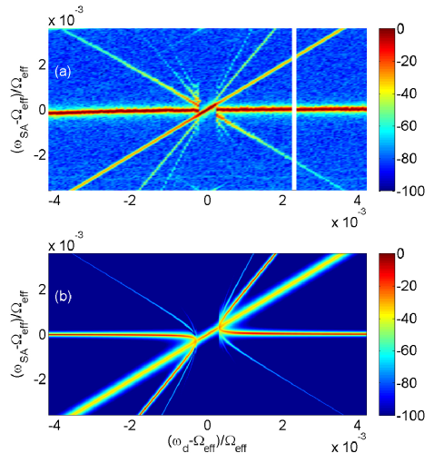
Figure 2: Power spectrum (in dB units) vs. detuning. (a) The measured power spectrum as a function of $\left(\omega_{\mathrm{d}}-\Omega_{\mathrm{eff}}\right)/\Omega_{\mathrm{eff}}$, where $\Omega_{\mathrm{eff}}/2\pi=236.4\operatorname{kHz}$. In this measurement the average laser power is set to $P_{\mathrm{L}}=12\operatorname{mW}$, the wavelength to $\lambda=1545.498\operatorname{nm}$ and the dimensionless laser modulation amplitude to $0.025$. (b) Theoretical calculation of the power spectrum based on the solution of Eq. (4). In both plots synchronization occurs when $\left|i_{\mathrm{b}}\right|<1$ and sidebands are observed when $\left|i_{\mathrm{b}}\right|>1$.

For the data presented in Fig. 2(a) synchronization occurs when $\omega_{\mathrm{d}}/\Omega_{\mathrm{eff}}\simeq 1$. Similar synchronization is observed when the ratio $\omega_{\mathrm{d}}/\Omega_{\mathrm{eff}}$ is tuned close to other rational values Shlomi_032910 ; Wang_023007 . As an example, the measured power spectrum for the case where $\omega_{\mathrm{d}}/\Omega_{\mathrm{eff}}\simeq 1/2$ is shown in Fig. 3. As can be seen from the comparison with Fig. 2(a), the results are qualitatively similar. Not shown here, but very similar behaviors were also experimentally observed at other ratios including $\omega_{\mathrm{d}}/\Omega_{\mathrm{eff}}\simeq 1/3$, $2/3$, $1/4$, $3/4$, $1/5$, $2/5$, $3/5$ and $4/5$. This highlights universal aspects of the phase-locking phenomenon when the drive frequency approximately matches a rational multiple of the natural self-oscillation frequency.

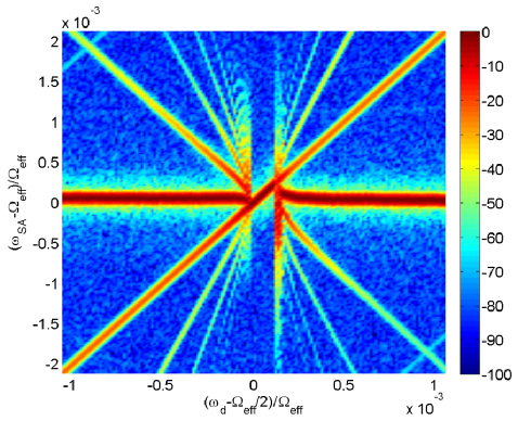
Figure 3: Measured power spectrum (in dB units) vs. detuning for the case where $\omega_{\mathrm{d}}/\Omega_{\mathrm{eff}}\simeq 1/2$. Other experimental parameters are listed in the caption of Fig. 2.

Phase locking near rational values of the ratio $\omega_{\mathrm{d}}/\Omega_{\mathrm{eff}}$ is qualitatively discussed in appendix C. It is found that just outside the locking regime the frequency of oscillation undergoes a transition from a value dictated by the externally applied modulation to the value corresponding to free running SEO. Moreover, this transition is expected to obey a “square root law” for both integer and fractional values of the ratio $\omega_{\mathrm{d}}/\Omega_{\mathrm{eff}}$. That is, the unlocking occurs continuously, with the deviation between the oscillator frequency from the (fraction of) drive frequency depending on the control parameter $\delta$ (drive amplitude, or detuning) as $\propto\sqrt{|\delta-\delta_{c}|}$, where $\delta_{c}$ is the critical – “unlocking” – value of $\delta$. This universality in the behavior just outside locking regime is demonstrated by the similarity of the spectrum measured near different locking regions (see Figs. 2 and 3).

VII Resonance detection in the region of synchronization

The effect of noise, which is assumed to be weak, can be taken into account by linearizing Eq. (4), which becomes

$$\frac{\mathrm{d}\gamma_{\mathrm{n}}}{\mathrm{d}\tau}+\gamma_{\mathrm{n}}\cos\gamma=i_{\mathrm{n}}\;,$$ (5)

where $\gamma$ represents a solution in the noiseless case and $\gamma_{\mathrm{n}}$ is a fluctuating term added to $\gamma$ due to noise. For the case $\left|i_{\mathrm{b}}\right|<1$ one finds from the stationary solution of Eq. (4) that $\cos\gamma=\sqrt{1-i_{\mathrm{b}}^{2}}$. The power spectrum $S_{\gamma}\left(w\right)$ of $\gamma_{\mathrm{n}}$ as a function of the dimensionless angular frequency $w$ can be found using Eq. (5) and the autocorrelation function $\left\langle i_{\mathrm{n}}\left(\tau\right)i_{\mathrm{n}}\left(\tau^{\prime}\right)\right\rangle$

$$S_{\gamma}\left(w\right)=\frac{\Theta}{\pi\omega_{\mathrm{a}}r_{0}^{2}}\frac{1}{1-i_{\mathrm{b}}^{2}+w^{2}}\;.$$ (6)

The correlation function $C_{\gamma}\left(\tau^{\prime}\right)=\left\langle\gamma_{\mathrm{n}}\left(\tau+\tau^{\prime}\right)\gamma_{\mathrm{n}}\left(\tau\right)\right\rangle$ can be determined using the Wiener-Khinchine theorem

$$C_{\gamma}\left(\tau^{\prime}\right)=\int_{-\infty}^{\infty}\mathrm{d}w\;e^{iw\tau^{\prime}}S_{\gamma}\left(w\right)=\frac{\Theta e^{-\sqrt{1-i_{\mathrm{b}}^{2}}\left|\tau^{\prime}\right|}}{\omega_{\mathrm{a}}r_{0}^{2}\sqrt{1-i_{\mathrm{b}}^{2}}}\;,$$ (7)

and thus the following holds $\left\langle\exp\left(i\left(\gamma_{\mathrm{n}}\left(\tau+\tau^{\prime}\right)-\gamma_{\mathrm{n}}\left(\tau\right)\right)\right)\right\rangle=1-\gamma_{\mathrm{g}}\left|\tau^{\prime}\right|+O\left(\left|\tau^{\prime}\right|^{2}\right)$, where $\gamma_{\mathrm{g}}$, which is given by $\gamma_{\mathrm{g}}=\Theta/\omega_{\mathrm{a}}r_{0}^{2}$, is the jitter rate. Note that $\gamma_{\mathrm{g}}$ is independent on $i_{\mathrm{b}}$. In terms of the the energy $U_{0}$ stored in the mechanical resonator the dimensionfull jitter rate is given by $\omega_{\mathrm{a}}\gamma_{\mathrm{g}}=\left(k_{\mathrm{B}}T_{\mathrm{eff}}/U_{0}\right)\gamma_{0}$. Note that the same jitter rate is obtained for the case of FO (provided that $U_{0}$ is unchanged).

In the region of synchronization, i.e. when $\left|i_{\mathrm{b}}\right|<1$, the resonance frequency $\Omega_{\mathrm{eff}}$ can be determined by monitoring the relative phase $\gamma$. Consider an estimate of the averaged value of $\gamma$ based on a sampling of the signal $\gamma+\gamma_{\mathrm{n}}\left(\tau\right)$ over a sampling time of duration $\tau_{\mathrm{a}}$. The standard deviation $\delta_{\gamma}$ in this estimate is given by

$$\delta_{\gamma}=\left(\frac{2\pi S_{\gamma}\left(0\right)}{\tau_{\mathrm{a}}}\right)^{1/2}=\left(\frac{2\Theta}{\omega_{\mathrm{a}}\tau_{\mathrm{a}}r_{0}^{2}\left(1-i_{\mathrm{b}}^{2}\right)}\right)^{1/2}\;.$$ (8)

The corresponding deviation $\delta_{\Omega}$ in the estimated value of $\Omega_{\mathrm{eff}}$ is given by $\delta_{\Omega}=\mathcal{R}\delta_{\gamma}$, where the responsivity $\mathcal{R}$ is given by $\mathcal{R}=\left(\left|\mathrm{d}\gamma/\mathrm{d}\Omega_{\mathrm{eff}}\right|\right)^{-1}=\omega_{\mathrm{a}}\sqrt{1-i_{\mathrm{b}}^{2}}$ , and thus the normalized minimum detectable change in the frequency is given by $\delta_{\Omega}/\Omega_{\mathrm{H}}=\sigma_{\mathrm{{\omega}0}}$, where $\sigma_{\mathrm{{\omega}0}}$ is given by Eq. (1). Thus for the same given stored energy $U_{0}$ in the mechanical resonator the same sensitivity is expected in the regions of synchronization and FO. In other words, the above-discussed degradation in sensitivity occurring in the region of SEO [see Eq. (3)] can be fully eliminated by synchronization-induced suppression of phase noise. Similarly to the case of FO, in the regime of synchronization the phase of mechanical oscillation is externally dictated, and consequently noise is suppressed.

VIII Summary

In summary, the sensitivity of a detector based on a mechanical resonator is studied in the SEO regime. It is found that phase noise can be suppressed by externally applying a modulation. Moreover, the transition from the regions of synchronization and free running SEO is explored, and a universal behavior referred to as the square-root law is revealed.

IX Acknowledgements

On-fiber optomechanical cavities have been fabricated by former members of the Technion group K. Shlomi, D. Yuvaraj and I. Baskin. Argonne National Laboratory’s contribution is based upon work supported by Laboratory Directed Research and Development (LDRD) funding from Argonne National Laboratory, provided by the Director, Office of Science, of the U.S. Department of Energy under Contract No. DE-AC02-06CH11357.

Appendix A Evolution equation

The theoretical model Zaitsev_1589 ; Zaitsev_046605 that is used to derive the evolution equation (2) is briefly described below. The micromechanical mirror in the optical cavity is treated as a mechanical resonator with a single degree of freedom $x$ having mass $m$ and linear damping rate $\gamma_{0}$ (when it is decoupled from the optical cavity). It is assumed that the angular resonance frequency of the mechanical resonator depends on the temperature $T$ of the suspended mirror. For small deviation of $T$ from the base temperature $T_{0}$ (i.e. the temperature of the supporting substrate) it is taken to be given by $\omega_{0}-\beta T_{\mathrm{R}}$, where $T_{\mathrm{R}}=T-T_{0}$ and where $\beta$ is a constant. Furthermore, to model the effect of thermal deformation Metzger_133903 it is assumed that a temperature dependent force given by $m\theta T_{\mathrm{R}}$, where $\theta$ is a constant, acts on the mechanical resonator Yuvaraj_430 . When noise is disregarded, the equation of motion governing the dynamics of the mechanical resonator is taken to be given by

$$\frac{\mathrm{d}^{2}x}{\mathrm{d}t^{2}}+2\gamma_{0}\frac{\mathrm{d}x}{\mathrm{d}t}+\left(\omega_{0}-\beta T_{\mathrm{R}}\right)^{2}x=\theta T_{\mathrm{R}}\;.$$ (9)

The intra-cavity optical power incident on the suspended mirror is denoted by $P_{\mathrm{L}}I\left(x\right)$, where $P_{\mathrm{L}}$ is the injected laser power, and the function $I\left(x\right)$ depends on the mechanical displacement $x$ [see Eq. (11) below]. The time evolution of the relative temperature $T_{\mathrm{R}}$ is governed by the thermal balance equation

$$\frac{\mathrm{d}T_{\mathrm{R}}}{\mathrm{d}t}=Q-\kappa T_{\mathrm{R}}\;,$$ (10)

where $Q=\eta P_{\mathrm{L}}I\left(x\right)$ is proportional to the heating power, $\eta$ is the heating coefficient due to optical absorption and $\kappa$ is the thermal decay rate.

The function $I\left(x\right)$ depends on the properties of the optical cavity that is formed between the suspended mechanical mirror and the on-fiber static reflector. The finesse of the optical cavity is limited by loss mechanisms that give rise to optical energy leaking out of the cavity. The main escape routes are through the on-fiber static reflector, through absorption by the metallic mirror, and through radiation. The corresponding transmission probabilities are respectively denoted by $\mathcal{T}_{\mathrm{B}}$, $\mathcal{T}_{\mathrm{A}}$ and $\mathcal{T}_{\mathrm{R}}$. In terms of these parameters, the function $I\left(x\right)$ is given by Zaitsev_046605

$$I\left(x\right)=\frac{\beta_{\mathrm{F}}\left(1-\frac{\beta_{-}^{2}}{\beta_{+}^{2}}\right)\beta_{+}^{2}}{1-\cos\frac{4\pi x_{\mathrm{D}}}{\lambda}+\beta_{+}^{2}}\;,$$ (11)

where $x_{\mathrm{D}}=x-x_{\mathrm{R}}$ is the displacement of the mirror relative to a point $x_{\mathrm{R}}$, at which the energy stored in the optical cavity in steady state obtains a local maximum, $\beta_{\pm}^{2}=\left(\mathcal{T}_{\mathrm{B}}\pm\mathcal{T}_{\mathrm{A}}\pm\mathcal{T}_{\mathrm{R}}\right)^{2}/8$ and where $\beta_{\mathrm{F}}$ is the cavity finesse. The reflection probability $R_{\mathrm{C}}=P_{\mathrm{R}}/P_{\mathrm{L}}$ is given in steady state by Yurke_5054 ; Zaitsev_046605 $R_{\mathrm{C}}=1-I\left(x\right)/\beta_{\mathrm{F}}$. For sufficiently small $x$, the expansion $I\left(x\right)=I_{0}+I_{0}^{\prime}x+\left(1/2\right)I_{0}^{\prime\prime}x^{2}+O\left(x^{3}\right)$ can be employed, where a prime denotes differentiation with respect to the displacement $x$.

Consider the case where the laser power $P_{\mathrm{L}}$ is modulated in time according to $P_{\mathrm{L}}\left(t\right)=P_{0}+P_{1}\left(t\right)$, where $P_{0}$ is a constant and $P_{1}\left(t\right)$ is assumed to have a vanishing average. When both $P_{1}$ and $I-I_{0}$ are sufficiently small, the problem can be significantly simplified by employing the approximation $Q\simeq\eta P_{0}I+\eta P_{1}I_{0}$. The displacement $x\left(t\right)$ is expressed in terms of the complex amplitude $A$ as $x\left(t\right)=x_{0}+2\operatorname{Re}A$, where $x_{0}$, which is given by $x_{0}=\eta\theta P_{0}I_{0}/\kappa\omega_{0}^{2}$, is the averaged optically-induced static displacement. For a small displacement, the evolution equation for the complex amplitude $A$ is found to be given by Eq. (2) Zaitsev_1589 ; Shlomi_032910 , where both the effective resonance frequency $\Omega_{\mathrm{eff}}$ and the effective damping rate $\Gamma_{\mathrm{eff}}$ are real even functions of $\left|A\right|$. To second order in $\left|A\right|$ they are given by $\Gamma_{\mathrm{eff}}=\Gamma_{0}+\Gamma_{2}\left|A\right|^{2}$ and $\Omega_{\mathrm{eff}}=\Omega_{0}+\Omega_{2}\left|A\right|^{2}$, where $\Gamma_{0}=\gamma_{0}+\eta\theta P_{0}I_{0}^{\prime}/2\omega_{0}^{2}$, $\Gamma_{2}=\gamma_{2}+\eta\beta P_{0}I_{0}^{\prime\prime}/4\omega_{0}$, $\gamma_{2}$ is the intrinsic mechanical nonlinear quadratic damping rate Zaitsev_859 , $\Omega_{0}=\omega_{0}-\eta\beta P_{0}I_{0}/\kappa$ and $\Omega_{2}=-\eta\beta P_{0}I_{0}^{\prime\prime}/\kappa$. Note that the above expressions for $\Gamma_{\mathrm{eff}}$ and $\Omega_{\mathrm{eff}}$ are obtained by making the following assumptions: $\kappa^{2}/\omega_{0}^{3}\lambda\ll\beta/\theta\ll 1/2\omega_{0}x_{0}$ and $\kappa\ll\omega_{0}$, both typically hold experimentally Zaitsev_046605 . The term $\xi\left(t\right)$ in Eq. (2) represents the thermal force that is generated due to the laser power modulation. For the case of a monochromatic modulation at angular frequency $\omega_{\mathrm{d}}\simeq\Omega_{\mathrm{eff}}$ it is given by $\xi\left(t\right)=\eta P_{1}I_{0}\theta\Omega_{0}^{-2}e^{-i\omega_{\mathrm{d}}t}$.

Appendix B Monochromatic modulation with $\omega_{\mathrm{d}}\simeq\Omega_{\mathrm{eff}}$

In cylindrical coordinates the complex amplitude of mechanical oscillation $A$ is expressed as $A=A_{r}e^{iA_{\theta}}$, where $A_{r}=\sqrt{A_{x}^{2}+A_{y}^{2}}$ is positive, $A_{\theta}$ is real Hempstead_350 , and Eq. (2) is written as

$$\dot{A}_{r}+A_{r}\Gamma_{\mathrm{eff}}=\xi_{r}+\vartheta_{r}\;,$$ (12)

and

$$\dot{A}_{\theta}+\Omega_{\mathrm{eff}}\left(A_{r}\right)=\frac{\xi_{\theta}+\vartheta_{\theta}}{A_{r}}\;,$$ (13)

where

$$\xi_{r} =\frac{A_{x}\xi_{x}+A_{y}\xi_{y}}{A_{r}}\;,$$ (14)

$$\vartheta_{r} =\frac{A_{x}\vartheta_{x}+A_{y}\vartheta_{y}}{A_{r}}\;,$$ (15)

$$\xi_{\theta} =\frac{A_{x}\xi_{y}-A_{y}\xi_{x}}{A_{r}}\;,$$ (16)

$$\vartheta_{\theta} =\frac{A_{x}\vartheta_{y}-A_{y}\vartheta_{x}}{A_{r}}\;,$$ (17)

$A=A_{x}+iA_{y}$, $\xi=\xi_{x}+i\xi_{y}$, where $A_{x}$, $A_{y}$, $\xi_{x}$ and $\xi_{y}$ are all real, and the noise terms satisfy the following relations

$$\left\langle\vartheta_{r}\left(t\right)\vartheta_{r}\left(t^{\prime}\right)\right\rangle =2\Theta\delta\left(t-t^{\prime}\right)\;,$$ (18)

$$\left\langle\vartheta_{\theta}\left(t\right)\vartheta_{\theta}\left(t^{\prime}\right)\right\rangle =2\Theta\delta\left(t-t^{\prime}\right)\;,$$ (19)

$$\left\langle\vartheta_{r}\left(t\right)\vartheta_{\theta}\left(t^{\prime}\right)\right\rangle =0\;.$$ (20)

Consider the case of a monochromatic modulation at angular frequency $\omega_{\mathrm{d}}$, which is assumed to be close to the angular frequency $\Omega_{\mathrm{eff}}$. When fluctuations in the amplitude $A_{r}$ of SEO are disregarded, i.e. when it is assumed that $A_{r}=r_{0}$, Eq. (13) becomes [see Eq. (16)]

$$\dot{A}_{\theta}+\Omega_{\mathrm{eff}}=-\omega_{\mathrm{a}}\sin\left(A_{\theta}+\omega_{\mathrm{d}}t\right)+\frac{\vartheta_{\theta}}{r_{0}}\;,$$ (21)

where $\Omega_{\mathrm{eff}}\$is treated as a constant and where $\omega_{\mathrm{a}}$, which is given by $\omega_{\mathrm{a}}=\eta P_{1}I_{0}\theta/\Omega_{0}^{2}r_{0}$, represents the modulation amplitude. In terms of the relative phase $\gamma=A_{\theta}+\omega_{\mathrm{d}}t$ and the dimensionless time $\tau=\omega_{\mathrm{a}}t$ Eq. (21) can be rewritten as

$$\frac{\mathrm{d}\gamma}{\mathrm{d}\tau}+\sin\gamma=i_{\mathrm{b}}+i_{\mathrm{n}}\;,$$ (22)

where

$$i_{\mathrm{b}}=\frac{\omega_{\mathrm{d}}-\Omega_{\mathrm{eff}}}{\omega_{\mathrm{a}}}\;,$$ (23)

and where $i_{\mathrm{n}}=\vartheta_{\theta}/\left(\omega_{\mathrm{a}}r_{0}\right)$. With the help of Eq. (19) one finds that

$$\left\langle i_{\mathrm{n}}\left(\tau\right)i_{\mathrm{n}}\left(\tau^{\prime}\right)\right\rangle=\frac{2\Theta}{\omega_{\mathrm{a}}r_{0}^{2}}\delta\left(\tau-\tau^{\prime}\right)\;.$$ (24)

B.1 The noiseless case

Consider first the noiseless case, for which $i_{\mathrm{n}}=0$. Below the time evolution of $\gamma$ in the region $\left|i_{\mathrm{b}}\right|>1$ is derived. Rewriting Eq. (22) as $\mathrm{d}\tau=\mathrm{d}\gamma/\left(i_{\mathrm{b}}-\sin\gamma\right)$ leads by integration to

$$\tau=\frac{2}{\sqrt{i_{\mathrm{b}}^{2}-1}}\tan^{-1}\frac{i_{\mathrm{b}}\tan\frac{\gamma}{2}-1}{\sqrt{i_{\mathrm{b}}^{2}-1}}\;.$$ (25)

Inverting this relation yields

$$\gamma=2\tan^{-1}\frac{1+\sqrt{i_{\mathrm{b}}^{2}-1}\tan\frac{\pi\tau}{T_{\mathrm{J}}}}{i_{\mathrm{b}}}\;,$$ (26)

where the normalized period time $T_{\mathrm{J}}$ is given by

$$T_{\mathrm{J}}=\frac{2\pi}{\sqrt{i_{\mathrm{b}}^{2}-1}}\;,$$ (27)

and thus

$$A_{\theta}=2\tan^{-1}\frac{1+\sqrt{i_{\mathrm{b}}^{2}-1}\tan\left(\frac{\sqrt{i_{\mathrm{b}}^{2}-1}\omega_{\mathrm{a}}}{2\omega_{\mathrm{d}}}\omega_{\mathrm{d}}t\right)}{i_{\mathrm{b}}}-\omega_{\mathrm{d}}t\;.$$ (28)

The averaged derivative $\left\langle\mathrm{d}\gamma/\mathrm{d}\tau\right\rangle$ is related to the period time $T_{\mathrm{J}}$ by

$$\left\langle\frac{\mathrm{d}\gamma}{\mathrm{d}\tau}\right\rangle=\frac{1}{T_{\mathrm{J}}}\int_{0}^{T_{\mathrm{J}}}\frac{\mathrm{d}\gamma}{\mathrm{d}\tau}\mathrm{d}\tau=\frac{2\pi}{T_{\mathrm{J}}}\;,$$ (29)

thus [see Eqs. (23) and (27)]

$$\left\langle\frac{\mathrm{d}\gamma}{\mathrm{d}\tau}\right\rangle=\sqrt{i_{\mathrm{b}}^{2}-1}\;,$$ (30)

and

$$-\left\langle\frac{\mathrm{d}A_{\theta}}{\mathrm{d}t}\right\rangle=\left\{\begin{array}[c]{cc}\omega_{\mathrm{d}}&\left|i_{\mathrm{b}}\right|<1\\ \omega_{\mathrm{d}}-\omega_{\mathrm{a}}\sqrt{i_{\mathrm{b}}^{2}-1}&\left|i_{\mathrm{b}}\right|\geq 1\end{array}\right.\;.$$ (31)

Therefore, the signal $\cos A_{\theta}$ when $\left|i_{\mathrm{b}}\right|\geq 1$ has Fourier spectrum made of peaks at the angular frequencies $\omega_{\mathrm{d}}+n\omega_{\mathrm{s}}$, where $n$ is an integer and the sideband spacing $\omega_{\mathrm{s}}$, which is given by $\omega_{\mathrm{s}}=2\pi\omega_{\mathrm{a}}/T_{\mathrm{J}}=\sqrt{\left(\omega_{\mathrm{d}}-\Omega_{\mathrm{eff}}\right)^{2}-\omega_{\mathrm{a}}^{2}}$ [see Eqs. (23) and (27)], depends on both the amplitude $\omega_{\mathrm{a}}$ and frequency $\omega_{\mathrm{d}}$ of the forcing term $\xi=r_{0}\omega_{\mathrm{a}}A_{r}e^{-i\omega_{\mathrm{d}}t}$.

B.2 Fourier expansion

With the help of Eqs. (22), (26) and (27) together with the identity $\sin\left(2\tan^{-1}\left(s\right)\right)=2s/\left(1+s^{2}\right)$ one finds that

$$\frac{\mathrm{d}\gamma}{\mathrm{d}\tau}=\mathcal{V}\left(\frac{2\pi\tau}{T_{\mathrm{J}}}+x_{0}\right)\;,$$ (32)

where the function $\mathcal{V}\left(x\right)$ is defined by

$$\mathcal{V}\left(x\right)=\frac{i_{\mathrm{b}}^{2}-1}{i_{\mathrm{b}}+\sin x}\;,$$ (33)

and where

$$x_{0}=\tan^{-1}\frac{1}{\sqrt{i_{\mathrm{b}}^{2}-1}}\;.$$ (34)

The Fourier expansion of the function $\mathcal{V}\left(x\right)$ is expressed as [see Eq. (33)]

$$\mathcal{V}\left(x\right)=\sum\limits_{k=-\infty}^{\infty}g_{k}e^{ikx}\;,$$ (35)

where

$$g_{k}=\frac{i_{\mathrm{b}}}{\left|i_{\mathrm{b}}\right|}\sqrt{i_{\mathrm{b}}^{2}-1}i^{k}\left(i_{\mathrm{b}}-\frac{i_{\mathrm{b}}}{\left|i_{\mathrm{b}}\right|}\sqrt{i_{\mathrm{b}}^{2}-1}\right)^{\left|k\right|}\;.$$ (36)

Thus, the magnitude of the sideband peaks is relatively large when $\left|i_{\mathrm{b}}\right|\gtrsim 1$. For $\left|i_{\mathrm{b}}\right|\gg 1$ the sidebands become small, and the relative phase becomes $\gamma\simeq\left(\omega_{\mathrm{d}}-\Omega_{\mathrm{eff}}\right)t$ [see Eq. (26)], i.e. the effect of laser modulation becomes weak.

Appendix C Square root law

In each of the regions of phase locking Paciorek_1723 ; Adler_351 the so-called winding number, which measures the oscillator phase accumulation relative to the phase of the drive, shows a plateau Jensen_1637 ; Ben-Jacob_822 ; Reichhardt_414 ; Shim_95 . For concreteness, consider the region just outside the primary plateau where (for positive $i_{\mathrm{b}}$) $0<i_{\mathrm{b}}-1\ll 1$, where $i_{\mathrm{b}}$ is the normalized detuning (recall that $\left|i_{\mathrm{b}}\right|=1$ at the onset of synchronization). The dimensionless frequency $T_{\mathrm{J}}^{-1}$ in this region is related to the critical parameter $i_{\mathrm{b}}-1$ by $T_{\mathrm{J}}^{-1}\simeq 2^{-1/2}\pi^{-1}\sqrt{i_{\mathrm{b}}-1}$ [see Eq. (27)]. Below it is shown that a similar ’square root law’ can be obtained for the region just outside any other plateau.

Consider a general 1D map having the form

$$\theta_{n+1}=\theta_{n}-\alpha+{W_{\mathrm{a}}\mathcal{F}\left(\theta_{n}\right)}\;,$$ (37)

that describes, e.g. the phase of the oscillator motion observed every period of the applied drive. The detuning $\alpha$ is approximately $(\Omega_{\mathrm{eff}}-\omega_{\mathrm{d}})2\pi/\omega_{\mathrm{d}}$. $W_{\mathrm{a}}$ parametrizes the strength of applied periodic drive (zero in the absence of drive). The “map function” is a periodic real function, if we assume that the phase at the sampling step $n+1$ only depends on phase at step $n$, and the phases $\theta$ and $\theta+2\pi$ are physically indistinguishable, $\mathcal{F}\left(\theta+2\pi\right)=\mathcal{F}\left(\theta\right)$.

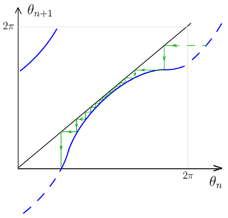
Figure 4: Phase locking-unlocking transition. Blue line represents mapping of Eq. (37), on the unlocked side of the transition. Green line is the staircase diagram that bounces between the map function and the diagonal $\theta_{n+1}=\theta_{n}$, graphically implementing the iteration procedure. Note that most of the iterations (longest time) is spend around the near-touching region. This leads to the “square-root” law for the splitting between the drive frequency and the oscillator frequency.

If the drive frequency is near the oscillator frequency, then the detuning is close to zero. The phase locking corresponds to a stable fixed point of the map, which can be found by solving the equation $\theta_{n+1}=\theta_{n}\equiv\theta^{*}$, that is

$$\alpha={W_{\mathrm{a}}\mathcal{F}\left(\theta^{*}\right)}\;,$$ (38)

where $\theta^{*}$ is the stroboscopic value of the oscillator phase at the fixed point. Since the function $\cal F$ is continuous and periodic, it is bounded, and the fixed point of this map only exists for a small enough detuning.

Suppose now that the drive frequency is an integer fraction of the oscillator frequency, $\omega_{\mathrm{d}}\approx\Omega_{\mathrm{eff}}/p$. Then, since the phase is defined modulo $2\pi$, the effective detuning in this case is still small and the analysis of the locking transition is based on the same map equation. The locking will occur to $\Omega_{\mathrm{eff}}=p\omega_{\mathrm{d}}$ On the other hand, if the frequency of the drive is an integer multiple ($\omega_{\mathrm{d}}\approx p\Omega_{\mathrm{eff}}$) of the oscillator frequency, then during one period of the drive, oscillator will only accrue a fraction $\approx 2\pi/p$ phase, which in general will correspond to too large of a detuning over single period of the drive to allow for a fixed point solution. However, the problem can be reduced to a formally equivalent one by iterating the map $p$ times,

$$\theta_{n+p}=\theta_{n}-p\alpha+{\tilde{W}_{\mathrm{a}}\mathcal{\tilde{F}}\left(\theta_{n}\right)}\;,$$ (39)

where the effective detuning $p\alpha$ is now close to $2\pi$, and the original treatment for the simple locking applies, with the resulting locked frequency being $\Omega_{\mathrm{eff}}=\omega_{\mathrm{d}}/p$. Note however, that the amplitude and the form of the map function are now different, and generically smaller in magnitude that the $p=1$ case. This makes locking to high frequency drives in general less stable.

Now, let us look more carefully at the transition out of the locking regime as a function of detuning, $\alpha$. Let us define $\alpha_{c}$ as the value of detuning and $\theta_{c}$ as the value of the fixed point $\theta^{*}$ at the transition between locked and the running phase (unlocked) regimes, $\theta_{c}=\theta^{*}(\alpha_{c})$. At the critical detuning, the slope of the map function $\cal F$ vanishes (see Figure 4). We can expand the map function around this point up to the second order,

$$\mathcal{F}\left(\theta\right)=\frac{\alpha_{\mathrm{c}}}{W_{\mathrm{a}}}\left[1-z^{2}\left(\theta-\theta_{\mathrm{c}}\right)^{2}\right]+O\left(\left(\theta-\theta_{\mathrm{c}}\right)^{3}\right)\;,$$ (40)

where $z$ is a parameter that characterizes the curvature of the map function near $\theta_{c}$. Indeed, as can be seen from Eq. (37), the map has a fixed point (i.e. a solution to the equation $\theta_{n+1}=\theta_{n}$) provided that $\alpha<\alpha_{\mathrm{c}}$ (the fixed point is given by $\theta^{*}=\theta_{\mathrm{c}}+\sqrt{1-\alpha/\alpha_{\mathrm{c}}}/z$).

On the unlocked side, it is convenient to treat the discreet series $y_{n}=\theta_{n}-\theta_{\mathrm{c}}$ as a continuous function $y\left(n\right)$, since near $\theta_{c}$ each iteration step changes $\theta$ only slightly (“staircase” diagram in Figure 4). Then, from (37) and (40)

$$\frac{\mathrm{d}y}{\mathrm{d}n}=\alpha_{\mathrm{c}}-\alpha-\alpha_{\mathrm{c}}z^{2}y^{2}\;.$$ (41)

This equation can be easily integrated in order to determine how long it takes the phase to pass through the bottleneck (Fig. 4). For that, the limits of integration over $y$ can be extended to the full real axis (details of the map function away from $\theta_{c}$ do not matter in this regime, since it takes much shorter time to go through regions other than the bottleneck).

Thus the estimate for the total number of drive periods for the phase to wind by $2\pi$ relative to the drive, is

$$N(\alpha) =\frac{1}{\alpha-\alpha_{\mathrm{c}}}\int_{-\infty}^{\infty}\frac{\mathrm{d}y}{1+\frac{\alpha_{\mathrm{c}}}{\alpha-\alpha_{\mathrm{c}}}z^{2}y^{2}}$$

$$=\frac{\pi}{z\sqrt{\alpha_{\mathrm{c}}|\alpha-\alpha_{\mathrm{c}}|}}\;.$$

This translates into the time period $T_{\mathrm{LC}}=2\pi N(\alpha)/\omega_{d}$ per $2\pi$ phase slip. Thus, the periodic oscillation of $y$ gives rise to sideband spectral peaks split from the drive frequency by integer multiples of $2\pi/T_{\mathrm{LC}}\propto\sqrt{|\alpha-\alpha_{\mathrm{c}}|}$.

References

- (1) A. N. Cleland and M. L. Roukes, “Noise processes in nanomechanical resonators,” J. Appl. Phys., vol. 92, no. 5, pp. 2758–2769, Sep 2002.
- (2) E. Buks, S. Zaitsev, E. Segev, B. Abdo, and M. P. Blencowe, “Displacement detection with a vibrating RF SQUID: Beating the standard linear limit,” Phys. Rev. E, vol. 76, p. 26217, 2007.
- (3) D. Rugar, H. J. Mamin, and P. Guethner, “Improved fiber-optic interferometer for atomic force microscopy,” Applied Physics Letters, vol. 55, no. 25, pp. 2588–2590, 1989.
- (4) O. Arcizet, P.-F. Cohadon, T. Briant, M. Pinard, A. Heidmann, J.-M. Mackowski, C. Michel, L. Pinard, O. Français, and L. Rousseau, “High-sensitivity optical monitoring of a micromechanical resonator with a quantum-limited optomechanical sensor,” Phys Rev Lett, vol. 97, p. 133601, Sep 2006.
- (5) S. Forstner, S. Prams, J. Knittel, E. D. van Ooijen, J. D. Swaim, G. I. Harris, A. Szorkovszky, W. P. Bowen, and H. Rubinsztein-Dunlop, “Cavity optomechanical magnetometer,” Phys. Rev. Lett., vol. 108, p. 120801, Mar 2012.
- (6) S. Stapfner, L. Ost, D. Hunger, J. Reichel, I. Favero, and E. M. Weig, “Cavity-enhanced optical detection of carbon nanotube brownian motion,” Applied Physics Letters, vol. 102, no. 15, p. 151910, 2013.
- (7) V. Braginsky and A. Manukin, “Ponderomotive effects of electromagnetic radiation,” Soviet Physics JETP, vol. 25, p. 653, 1967.
- (8) K. Hane and K. Suzuki, “Self-excited vibration of a self-supporting thin film caused by laser irradiation,” Sensors and Actuators A: Physical, vol. 51, pp. 179–182, 1996.
- (9) S. Gigan, H. R. Böhm, M. Paternostro, F. Blaser, J. B. Hertzberg, K. C. Schwab, D. Bauerle, M. Aspelmeyer, and A.Zeilinger, “Self cooling of a micromirror by radiation pressure,” Nature, vol. 444, pp. 67–70, 2006.
- (10) C. H. Metzger and K.Karrai, “Cavity cooling of a microlever,” Nature, vol. 432, pp. 1002–1005, 2004.
- (11) T. J. Kippenberg and K. J. Vahala, “Cavity optomechanics: Back-action at the mesoscale,” Science, vol. 321, no. 5893, pp. 1172–1176, Aug 2008.
- (12) C. M. I. Favero, S. Camerer, D. Konig, H. Lorenz, J. P. Kotthaus, and K. Karrai, “Optical cooling of a micromirror of wavelength size,” Appl. Phys. Lett., vol. 90, p. 104101, 2007.
- (13) F. Marquardt and S. M. Girvin, “Optomechanics,” Physics, vol. 2, p. 40, May 2009.
- (14) S. E. Lyshevski and M. Lyshevski, “Nano- and microoptoelectromechanical systems and nanoscale active optics,” in Third IEEE Conference on Nanotechnology, 2003., vol. 2, Aug 2003, pp. 840–843.
- (15) N. Stokes, F. Fatah, and S. Venkatesh, “Self-excited vibrations of optical microresonators,” Electronics Letters, vol. 24, no. 13, pp. 777–778, 1988.
- (16) M. Hossein-Zadeh and K. J. Vahala, “An optomechanical oscillator on a silicon chip,” IEEE J. Sel. Top. Quantum Electron., vol. 16, no. 1, pp. 276–287, Jan 2010.
- (17) M. C. Wu, O. Solgaard, and J. E. Ford, “Optical MEMS for lightwave communication,” J. Lightwave Technol., vol. 24, no. 12, pp. 4433–4454, Dec 2006.
- (18) M. Eichenfield, C. P. Michael, R. Perahia, and O. Painter, “Actuation of micro-optomechanical systems via cavity-enhanced optical dipole forces,” Nature Photonics, vol. 1, p. 416, 2007.
- (19) G. Bahl, J. Zehnpfennig, M. Tomes, and T. Carmon, “Stimulated optomechanical excitation of surface acoustic waves in a microdevice,” Nature Communications, vol. 2:403, 2011. [Online]. Available: http://dx.doi.org/10.1038/ncomms1412
- (20) N. Flowers-Jacobs, S. Hoch, J. Sankey, A. Kashkanova, A. Jayich, C. Deutsch, J. Reichel, and J. Harris, “Fiber-cavity-based optomechanical device,” Applied Physics Letters, vol. 101, no. 22, p. 221109, 2012.
- (21) M. Poot and H. S. van der Zant, “Mechanical systems in the quantum regime,” Phys. Rep., vol. 511, pp. 273–335, 2012.
- (22) T. J. Kippenberg, H. Rokhsari, T. Carmon, A. Scherer, and K. J. Vahala, “Analysis of radiation-pressure induced mechanical oscillation of an optical microcavity,” Phys. Rev. Lett., vol. 95, p. 033901, July 2005.
- (23) H. Rokhsari, T. Kippenberg, T. Carmon, and K. Vahala, “Radiation-pressure-driven micro-mechanical oscillator,” Opt. Express, vol. 13, no. 14, pp. 5293–5301, Jul 2005.
- (24) O. Arcizet, P. F.Cohadon, T. Briant, M. Pinard, and A. Heidmann, “Radiation-pressure cooling and optomechanical instability of a micromirror,” Nature, vol. 444, pp. 71–74, 2006.
- (25) D. Kleckner and D. Bouwmeester, “Sub-kelvin optical cooling of a micromechanical resonator,” Nature, vol. 444, p. 75, 2006.
- (26) G. Jourdan, F. Comin, and J. Chevrier, “Mechanical mode dependence of bolometric backaction in an atomic force microscopy microlever,” Phys. Rev. Lett., vol. 101, p. 133904, Sep 2008.
- (27) F. Marino and F. Marin, “Chaotically spiking attractors in suspended-mirror optical cavities,” Phys. Rev. E, vol. 83, p. 015202, Jan 2011.
- (28) C. Metzger, M. Ludwig, C. Neuenhahn, A. Ortlieb, I. Favero, K. Karrai, and F. Marquardt, “Self-induced oscillations in an optomechanical system driven by bolometric backaction,” Phys. Rev. Lett., vol. 101, p. 133903, Sep 2008.
- (29) J. Restrepo, J. Gabelli, C. Ciuti, and I. Favero, “Classical and quantum theory of photothermal cavity cooling of a mechanical oscillator,” Comptes Rendus Physique, vol. 12, pp. 860–870, Nov 2011.
- (30) S. D. Liberato, N. Lambert, and F. Nori, “Quantum limit of photothermal cooling,” arXiv:1011.6295, Nov 2010.
- (31) F. Marquardt, J. G. E. Harris, and S. M. Girvin, “Dynamical multistability induced by radiation pressure in high-finesse micromechanical optical cavities,” Phys. Rev. Lett., vol. 96, p. 103901, 2006.
- (32) M. Paternostro, S. Gigan, M. S. Kim, F. Blaser, H. R. Böhm, and M. Aspelmeyer, “Reconstructing the dynamics of a movable mirror in a detuned optical cavity,” New J. Phys., vol. 8, p. 107, Jun 2006.
- (33) D. Yuvaraj, M. B. Kadam, O. Shtempluck, and E. Buks, “Optomechanical cavity with a buckled mirror,” JMEMS, vol. 22, p. 430, 2013.
- (34) K. Aubin, M. Zalalutdinov, T. Alan, R. Reichenbach, R. Rand, A. Zehnder, J. Parpia, and H. Craighead, “Limit cycle oscillations in CW laser-driven NEMS,” J. MEMS, vol. 13, pp. 1018–1026, 2004.
- (35) S. De Liberato, N. Lambert, and F. Nori, “Quantum noise in photothermal cooling,” Phys. Rev. A, vol. 83, p. 033809, Mar 2011.
- (36) S. Zaitsev, A. K. Pandey, O. Shtempluck, and E. Buks, “Forced and self-excited oscillations of optomechanical cavity,” Phys. Rev. E, vol. 84, p. 046605, 2011.
- (37) S. Zaitsev, O. Gottlieb, and E. Buks, “Nonlinear dynamics of a microelectromechanical mirror in an optical resonance cavity,” Nonlinear Dyn., vol. 69, pp. 1589–1610, 2012.
- (38) K. Kim and S. Lee, “Self-oscillation mode induced in an atomic force microscope cantilever,” J. Appl. Phys., vol. 91, pp. 4715–4719, 2002.
- (39) T. Carmon, H. Rokhsari, L. Yang, T. J. Kippenberg, and K. J. Vahala, “Temporal behavior of radiation-pressure-induced vibrations of an optical microcavity phonon mode,” Phys. Rev. Lett., vol. 94, p. 223902, 2005.
- (40) T. Corbitt, D. Ottaway, E. Innerhofer, J. Pelc, and N. Mavalvala, “Measurement of radiation-pressure-induced optomechanical dynamics in a suspended fabry-perot cavity,” Phys. Rev. A, vol. 74, p. 21802, 2006.
- (41) T. Carmon and K. J. Vahala, “Modal spectroscopy of optoexcited vibrations of a micron-scale on-chip resonator at greater than 1 ghz frequency,” Phys. Rev. Lett., vol. 98, p. 123901, 2007.
- (42) K. Shlomi, D. Yuvaraj, I. Baskin, O. Suchoi, R. Winik, and E. Buks, “Synchronization in an optomechanical cavity,” Physical Review E, vol. 91, no. 3, p. 032910, 2015.
- (43) H. Wang, Y. Dhayalan, and E. Buks, “Devil’s staircase in an optomechanical cavity,” Physical Review E, vol. 93, no. 2, p. 023007, 2016.
- (44) Y. Dhayalan, I. Baskin, K. Shlomi, and E. Buks, “Phase space distribution near the self-excited oscillation threshold,” Phys. Rev. Lett., vol. 112, p. 210403, May 2014.
- (45) D. Anderson, V. Mizrahi, T. Erdogan, and A. White, “Production of in-fibre gratings using a diffractive optical element,” Electronics Letters, vol. 29, no. 6, pp. 566–568, 1993.
- (46) V. Anishchenko and T. Vadivasova, “Synchronization of self-oscillations and noise-induced oscillations,” JOURNAL OF COMMUNICATIONS TECHNOLOGY AND ELECTRONICS C/C OF RADIOTEKHNIKA I ELEKTRONIKA, vol. 47, no. 2, pp. 117–148, 2002.
- (47) M. Pandey, R. H. Rand, and A. T. Zehnder, “Frequency locking in a forced mathieu–van der pol–duffing system,” Nonlinear Dynamics, vol. 54, no. 1-2, pp. 3–12, 2008.
- (48) L. Paciorek, “Injection locking of oscillators,” Proc IEEE, vol. 53, pp. 1723–1727, 196.
- (49) R. Adler, “A study of locking phenomena in oscillators,” Proc. IRE, vol. 34, pp. 351–357, 1946.
- (50) M. H. Jensen, P. Bak, and T. Bohr, “Complete devil’s staircase, fractal dimension, and universality of mode- locking structure in the circle map,” Phys. Rev. Lett., vol. 50, pp. 1637–1639, May 1983. [Online]. Available: http://link.aps.org/doi/10.1103/PhysRevLett.50.1637
- (51) S. Dos Santos and M. Planat, “Generation of 1/f noise in locked systems working in nonlinear mode,” Ultrasonics, Ferroelectrics and Frequency Control, IEEE Transactions on, vol. 47, no. 5, pp. 1147–1151, 2000.
- (52) R. Hamerly and H. Mabuchi, “Optical devices based on limit cycles and amplification in semiconductor optical cavities,” arXiv:1504.04410, 2015.
- (53) C. Huygens and H. Oscillatorium, “The pendulum clock,” Trans RJ Blackwell, The Iowa State University Press, Ames, 1986.
- (54) M. Rosenblum and A. Pikovsky, “Synchronization: from pendulum clocks to chaotic lasers and chemical oscillators,” Contemporary Physics, vol. 44, no. 5, pp. 401–416, 2003.
- (55) G. Heinrich, M. Ludwig, J. Qian, B. Kubala, and F. Marquardt, “Collective dynamics in optomechanical arrays,” Physical review letters, vol. 107, no. 4, p. 043603, 2011.
- (56) M. Dykman, X. Chu, and J. Ross, “Stationary probability distribution near stable limit cycles far from hopf bifurcation points,” Physical Review E, vol. 48, no. 3, p. 1646, 1993.
- (57) H. Risken, The Fokker-Planck Equation: Methods of Solution and Applications. Springer, 1996.
- (58) K. Y. Fong, M. Poot, X. Han, and H. X. Tang, “Phase noise of self-sustained optomechanical oscillators,” Physical Review A, vol. 90, no. 2, p. 023825, 2014.
- (59) I. Baskin, D.Yuvaraj, G. Bachar, K. Shlomi, O. Shtempluck, and E. Buks, “Optically induced self-excited oscillations in an on-fiber optomechanical cavity,” JMEMS, vol. 23, pp. 563–569, 2014.
- (60) H. A. Kramers, “Brownian motion in a field of force and the diffusion model of chemical reactions,” Physica, vol. 7, p. 284, 1940.
- (61) P. Hanggi, P. Talkner, and M. Borkovec, “Reaction-rate theory: Fifty years after kramers,” Rev. Mod. Phys., vol. 62, pp. 251–341, 1990.
- (62) M. Tinkham, Introduction to Superconductivity. Florida: Robert E. Krieger, 1975.
- (63) S. Kogan, Electronic noise and fluctuations in solids. Cambridge University Press, 2008.
- (64) Y. Levinson, “Quantum noise in a current-biased josephson junction,” Physical Review B, vol. 67, no. 18, p. 184504, 2003.
- (65) B. Yurke and E. Buks, “Performance of cavity-parametric amplifiers, employing kerr nonlinearites, in the presence of two-photon loss,” J. Lightwave Tech., vol. 24, pp. 5054–5066, 2006.
- (66) S. Zaitsev, O. Shtempluck, E. Buks, and O. Gottlieb, “Nonlinear damping in a micromechanical oscillator,” Nonlinear Dynamics, vol. 67, no. 1, pp. 859–883, 2012.
- (67) R. D. Hempstead and M. Lax, “Classical noise. vi. noise in self-sustained oscillators near threshold,” Phys. Rev., vol. 161, pp. 350–366, Sep 1967. [Online]. Available: http://link.aps.org/doi/10.1103/PhysRev.161.350
- (68) E. Ben-Jacob, Y. Braiman, R. Shainsky, and Y. Imry, “Microwave-induced devil’s staircase structure and chaotic behavior in current-fed josephson junctions,” Applied Physics Letters, vol. 38, no. 10, pp. 822–824, 1981.
- (69) C. Reichhardt and F. Nori, “Phase locking, devil’s staircases, farey trees, and arnold tongues in driven vortex lattices with periodic pinning,” Physical review letters, vol. 82, no. 2, p. 414, 1999.
- (70) S.-B. Shim, M. Imboden, and P. Mohanty, “Synchronized oscillation in coupled nanomechanical oscillators,” Science, vol. 316, no. 5821, pp. 95–99, 2007.