Toward a Complete Understanding of the Magellanic Stream Formation

Abstract

The Magellanic Clouds have lost most of their gas during their passage by the Milky Way, a property that has never been successfully modeled. Here we use accurate and mesh-free hydrodynamic simulations to reproduce the Magellanic Stream and the Magellanic Clouds in the frame of a ’ram-pressure plus collision’ model. This model reproduces many of the observed properties of the HI Stream including most of its density profile along its length and its dual filamentary structure. Besides this, ram-pressure combined with Kelvin-Helmholtz instabilities extracts amounts of ionized and HI gas consistent with those observed. The modeled scenario also reproduces the Magellanic Bridge, including the offset between young and old stars, and the collision between the Clouds, which is responsible of the very elongated morphology of the Small Magellanic Cloud along the line of sight. This model has solved most of the mysteries linked to the formation of the Magellanic Stream. The Leading Arm is not reproduced in the current model because it requires an alternative origin.

1 Introduction

If one was wearing special glasses to see the HI 21cm line, one would see the Milky Way (MW) disc and as the second largest structure in the sky, the Magellanic Stream (hereafter MS, Mathewson, Cleary & Murray, 1974), which subtends an angle of more than 200 degrees (Nidever et al., 2010, 2013). The Stream is linked to the Magellanic Clouds (MCs) and its formation is still challenging to explain. The MCs are likely at their first passage by the MW according to their proper motions from Hubble Space Telescope (${\it HST}$, Kallivayalil et al., 2013) and Gaia Data Releases 2 (DR2, Gaia Collaboration et al., 2018b). In the meantime, Fox et al. (2014) estimated to 2 $\times$ $10^{9}$ $M_{\odot}$ the total mass released by the progenitors of both Magellanic Stream (MS) and Leading Arm (LA), assuming both structures at 55 kpc. Observation from H${\alpha}$ emission (Barger et al., 2017) also leads to a similar amount of ionized gas mass. Further analysis by Richter et al. (2017) leads to an even larger value, 3 $\times$ $10^{9}$ $M_{\odot}$. Since the MS is likely reaching higher distances than the LA, it is quite conservative to consider 1-2 $\times$ $10^{9}$ $M_{\odot}$ for the sole contribution of the MS. Multiple photoionization and collisional ionization processes that might lead to the ionization of the gas have been explored in the literature, e.g., extragalactic background, hot gas, shock, conductive heating, turbulent mixing (D’Onghia & Fox, 2016; Barger et al., 2017). It has been also suggested by Bland-Hawthorn et al. (2013) that the Stream region below the South Galactic Pole (SGP) could be related to the past AGN activity at the Galactic Center. Orbital calculations from proper motions of the MCs indicate that they experienced a strong collision a few hundreds Myr ago (Kallivayalil et al., 2013), which formed the Magellanic Bridge (MB) linking them together.

Explanations of the MS can be classified into two broad families. One is the ’tidal’ model (Besla et al., 2012; Pardy, D’Onghia & Fox, 2018; Tepper-García et al., 2019) assuming that the MS is a tidal tail extracted from the Small Magellanic Cloud (SMC) after a collision with a very massive, 1.5-2.5 $\times$ $10^{11}$ $M_{\odot}$, Large Magellanic Cloud (LMC). The other is the ram-pressure models with moderate mass for the LMC, 3-20 $\times$ $10^{9}$ $M_{\odot}$ (Mastropietro et al., 2005; Hammer et al., 2015), which consider ram-pressure effects and may also account for a recent collision between the Clouds.

The circum-galactic medium (CGM) plays a crucial role on the infalling gas by producing ram-pressure and Kelvin-Helmholtz (K-H) instabilities. The CGM extends to hundreds of kpc and is made of multi-phase gases (Lehner et al., 2012; Richter et al., 2017), hot (Gupta et al., 2012; Miller & Bregman, 2013; Nakashima et al., 2018) and warm phases (Zheng et al., 2019) showing similarities with MW-mass galaxies studied by Werk et al. (2014) and Prochaska et al. (2017). Indirect evidences that the HI Magellanic System is affected by the CGM gas are among others, provided by the exceptionally shrunk HI LMC disc (Salem et al., 2015) and the pressure confined clouds in the Stream (Fox et al., 2005; Kalberla & Haud, 2006; For et al., 2014). As recalled by Fillingham et al. (2016), CGM gas at all temperatures contributes to strip and heat the infalling gas, and its density is in excess of a few $10^{-4}{\rm cm}^{-3}$, strongly affecting the MS. In such a condition, the low HI density LA, is unlikely to survive in the CGM as shown by Tepper-García et al. (2019), requiring another origin, such as stripped gas-rich dwarfs moving ahead of the MCs (Hammer et al., 2015).

Fillingham et al. (2016) convincingly showed that even large gas densities (3-10 $\times$ $10^{-4}{\rm cm}^{-3}$) in the CGM are unable to remove significant fractions of the gas in galaxies with total masses in excess to a few $10^{10}$ $M_{\odot}$, i.e., masses of the MCs in the ’tidal’ scenario. We then choose to follow the ’ram-pressure plus collision’ modeling of Hammer et al. (2015). Here, we use a hydrodynamic solver GIZMO (Hopkins, 2015), which accounts fairly for, e.g., K-H instabilities, conversely to GADGET2.

2 NUMERICAL SIMULATIONS AND INITIAL CONDITIONS

2.1 Initial Conditions for the Milky Way and the Magellanic Clouds

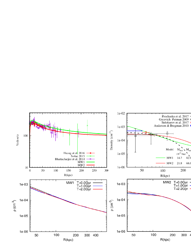
Figure 1: Top-left panel: comparison of the MW observed rotation data (Huang et al., 2016; Sofue, 2015; Bhattacharjee, Chaudhury & Kundu, 2014) and models used in this paper (red and green solid curves). Top-right panel: hot gas density profile used in models compared to several observational constraints, which are indicated on the top-right of the panel (see text). The cool CGM density profile based on Prochaska et al. (2017) is obtained by fitting their mass distribution with a Hernquist density profile with a core. Bottom panels: density profile evolution with time in isolation to test the stability of the two MW models.

The MW model is set up including a stellar disc, gas disc, hot gas halo, and dark matter halo. The stellar and gas disc have the same properties as in Hammer et al. (2015). For the hot gas halo, we use a core-profile similar to the halo profile of Hernquist (1993), which has large flexibility and well converging properties. Most constraints for the gaseous halo are indirect, based on observations at around 50 kpc as shown in the top-right panel of Fig. 1. In the current study, we use two types of hot gas halo profiles as shown by red and green lines (top-right panel of Fig. 1). Model MW1 shows a flatter profile since it includes the outskirt contribution of the IGM with a density of $\sim 2\times 10^{-5}$ cm^-3 at virial radius. For comparison, the observed cool CGM density profile of MW-mass galaxies (Prochaska et al., 2017) is also shown in Fig. 1. with a dashed-black line. The density profile has been calculated from the projected mass density distribution from Fig. 17 of Prochaska et al. (2017), assuming a core density profile (Hernquist, 1993). For the MW dark matter halo, we use a core model as in Barnes (2002), and the dark matter profile is then adjusted to fit the observed rotation curve, which is shown in the left panel of Fig. 1. Total and halo gas masses within the virial radius (260 kpc) are given in the top-right panel of Fig. 1 for the two adopted models. To reduce the particle number and numerical calculation in the simulation, the dark matter halo has been considered as causing a gravitational potential fully accounted by analytic formulae, such as: $\rho\propto(r+a_{\rm halo})^{-4}$ with $a_{\rm halo}$= 6 kpc and central density $\rho_{0}$= 0.7379 and 0.4919 M${}_{\odot}{\rm pc}^{-3}$ for MW1 and MW2, respectively.

To test the stability of the MW gas halo model, we run it in isolation for 2 Gyr, which is similar to the time duration during which the MCs simulations are made. The two panels in the bottom row of Fig. 1 show the hot gas density profile evolution over a 2 Gyr time scale. The two models of MW hot gas halo are stable enough for our studies.

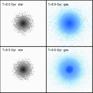
Figure 2: Projected density distribution of stars and gas for one model of the LMC at T$=0.0$ Gyr and after an evolution in isolation after 0.5 Gyr. The size of each panel is $100{\times}100$ kpc.

Table 1: Initial condition parameters

Model components	Model-27		Model-28		Model-52
	LMC	SMC	LMC	SMC	LMC	SMC
Stellar disc mass ($10^{9}$M⊙)	2.5	0.3	2.5	0.3	2.0	0.3
Gas disc mass ($10^{9}$M⊙)	2.5	2.4	2.5	2.4	2.0	2.4
Stellar Spheriod mass ($10^{9}$M⊙)	0	0.3	0	0.3	0	0.3
Scale-length of Stellar Disk (kpc)	1.4	1.5	1.4	1.5	1.4	1.5
Scaleheight of Stellar Disk (kpc)	1.0	0.8	1.0	0.8	1.0	0.8
Scale-length of gas Disk (kpc)	7.0	5.0	4.0	5.0	5.0	5.0
Scale size of Spheroid (kpc)	0.0	1.5	0.0	1.5	0.0	1.5
Number of Stellar Particles	150000	72000	300000	72000	240000	72000
Number of Gas Particles	150000	288000	300000	288000	240000	288000

The Large Magellanic Cloud, is assumed to be the combination of an exponential stellar disc with a neutral gas disc, for which the scale-length of the neutral gas disc is much larger than that of the stellar component as shown in Table 1 (van der Kruit, 2007; Pardy, D’Onghia & Fox, 2018; Tepper-García et al., 2019). For the Small Magellanic Cloud, we assume that there are two stellar components and one neutral gas disc. The stellar component consists of an exponential stellar disc and a spheroid, following Diaz & Bekki (2012). The stellar spheroid has a core density profile and is made of ancient stars, which is motivated by the recent observations of Ripepi et al. (2017) who found such a distribution using 3D mapping based on RR Lyrae stars. All the parameters used for the MCs are given in Table 1. The initial condition is created with a Schwarzschild orbit superposition method (Vasiliev, 2013; Vasiliev & Athanassoula, 2015). To test the stability of the initial model of the MCs, we let them evolve in isolation for 0.5 Gyr, without important changes as shown in Fig. 2. We have also tested cases after evolving MCs in isolation as progenitors, and the results do not change significantly. For both the MCs we have considered the possible presence of a dark matter halo. However their masses have been limited to be equal or up to 10 times the mass of the baryonic component that is few $10^{9}M_{\odot}$, since the MW CGM gas would not be able to extract the cold gas from more massive galaxies (Fillingham et al., 2016).

2.2 The Hydrodynamic Code GIZMO

The numerical simulations were carried out with GIZMO (Hopkins, 2015), which is based on a new Lagrangian method for hydrodynamics, and has simultaneously properties of both smoothed particle hydrodynamics (SPH) and grid-based/adaptive mesh refinement (AMR) methods. It has considerable advantages when compared to SPH, for instances, proper convergence, good capturing of fluid-mixing instabilities, dramatically reduced numerical viscosity, sharp shock capturing, and so on. These features make GIZMO providing a considerable advance when compared to GADGET-2, which was unable to properly account for K-H instabilities, considered by Hammer et al. (2015) as the main limitation for their study of the Magellanic Stream.

To use this code, we implemented into GIZMO star formation and feedback processes as in Wang et al. (2012) following the method of Cox et al. (2006). This code has been used for investigating the formation history of M31 (Hammer et al., 2018). For the radiative cooling process, we have used the updated version of Katz, Weinberg & Hernquist (1996). It assumes the gas as a primordial plasma, and ionization states of H and He are explicitly tracked under the assumption of collisional ionization equilibrium (Hopkins, 2015).

2.3 Convergence of the simulation

All the simulations are using a softening of 40 pc, which is large enough to minimize discreteness noise and also small enough to sample a reasonable resolution. The particles mass ratio between the hot gas of the MW and cold gas of the MCs are important for ram-pressure, which can result in spurious enhancement of ram-pressure stripping when this ratio is too large (Mastropietro et al., 2005; Kazantzidis et al., 2017; Abadi, Moore & Bower, 1999). In our simulations this ratio ranged from 2.4 to 12. To test convergence, we also run a high resolution simulation for Model-28, this ratio changed from 12 to 1.2, but our result did not change significantly, which indicate that our results are not affected by artificial effects.

2.4 Definition of Neutral Gas and Warm+Hot Gas

Since there is no radiative transfer used in the simulation, neutral and ionized gas can not be directly distinguished properly (Marasco et al., 2015). To compare the properties of neutral HI and warm+hot ionized gas stripped from the MCs with that from observations, we define particles with temperatures below 2 $\times$ $10^{4}$ K as neutral gas and assume simple collisional ionization equilibrium (Sutherland & Dopita, 1993), while particles with temperatures above 2 $\times$ $10^{4}$K are defined as warm+hot gas. The neutral hydrogen mass is derived by assuming that the gas has an universal hydrogen mass fraction of 0.76 (Sutherland & Dopita, 1993). This simple definition between neutral and ionized gas is consistent with studies of gas properties in simulations (Marasco et al., 2015; Sokołowska et al., 2016), and with observational conventions (Sokołowska et al., 2016; Putman, Peek & Joung, 2012).

2.5 Orbital Parameters

Determination of orbital parameters is a three-body problem (interaction between the two MCs and the MW), which is further complicated by gas dissipation properties. To calculate the initial position and velocity of the MCs before entering the MW hot medium, we use the solver defined by Yang & Hammer (2010) that has been improved in Hammer et al. (2015), and which can provide the final position and velocity of MCs at the current observing time and can match that of observations as shown in Sec. 3.

3 Results of Modeling

3.1 Gas Modeling

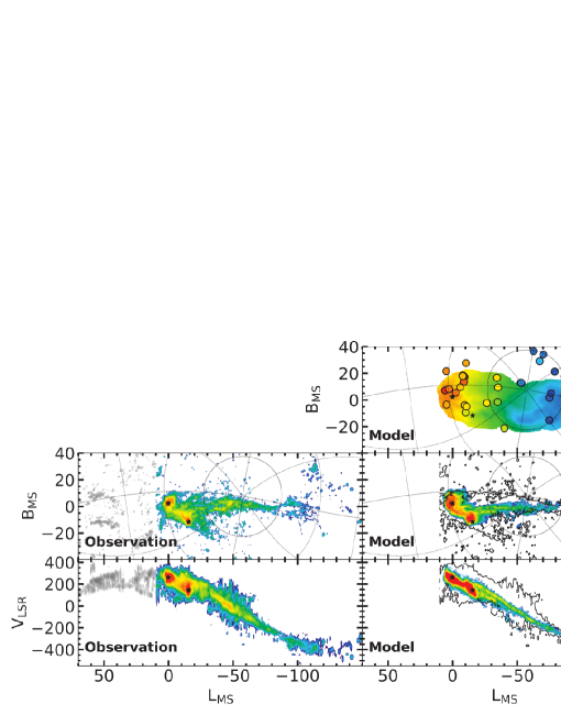
Figure 3: Comparing HI and warm+hot gas, from Model-28, distributions with observations in the Magellanic coordinate system (Nidever, Majewski & Butler Burton, 2008). The top right panel shows the sky distribution of the simulated warm+hot ionized gas with a color coding for the line of sight velocity. Points represent QSOs absorption line observations by HST/COS (Fox et al., 2014). The simulated ionized gas mass (0.81-0.94$\times$$10^{9}$M_⊙) is consistent with that observed ${\sim}10^{9}$M_⊙ (D’Onghia & Fox, 2016). Most of them are lying in the same area as the simulations, though observations indicate an even larger area for the ionized gas. The bottom two rows compare observed HI distributions of the Magellanic Stream with that of simulations, of which the left column are results of HI observations from Nidever et al. (2010), while the right column shows results from simulation of Model-28. The black stars in each panel indicate the position of LMC and SMC. The HI mass in the MS is in the range of 1.4-5${\times}10^{8}$M_⊙, which is consistent with observations, 2.7${\times}10^{8}$M_⊙ (D’Onghia & Fox, 2016). In the simulation panels observations are marked by contours. The LA is shown with grey color in the left side of the observation panel to indicate that it is not reproduced by our models, because it is assumed to have another origin rather than the MC gas (Yang et al., 2014; Hammer et al., 2015; Tepper-García et al., 2019).

In the current model, the MCs enter the gas corona of the MW and their HI content is stripped by ram-pressure effects, which result in the formation of the HI MS. Fig. 3 shows the HI sky distribution and its velocity along the Magellanic longitude. As in Hammer et al. (2015) the simulated HI Stream reproduces well the observations, including the two ram-pressure tails lagging behind each MC that mimic the MS structure with its two twisting filaments (Nidever et al., 2010). Observations of HI kinematics (Nidever, Majewski & Butler Burton, 2008) and chemical abundances (Fox et al., 2013; Richter et al., 2013) show that one of the two main filaments has LMC-like chemistry and kinematics, whereas the other has SMC-like properties. This indicates that one filament originates in the LMC, whereas the other originates in the SMC. This observed dual filamentary features is naturally formed by the ram-pressure stripping scenario, as ram-pressure acts separately on each Cloud, stripping gas to form two trailing stream tails of MCs (for a detailed comparison, see Hammer et al. 2015 and Fig. 5). The HI gas mass of the MS ranges from 1.4 to 5 $\times$ $10^{8}$M_⊙, to be compared to the observed value, 2.7 $\times$ $10^{8}$M_⊙ (D’Onghia & Fox, 2016). The two values are in good agreement, since the latter is likely underestimated by assuming a 55 kpc distance for all the MS extent. Moreover, the column density profile of the HI gas is well reproduced (see Sec.3.4).

The main difference with Hammer et al. (2015) modeling is the use of the GIZMO (Hopkins, 2015, 2017) hydrodynamic solver instead of GADGET2. The former code accounts for K-H instabilities far much better than GADGET2 (Hopkins, 2015), that do not only strips the MC gas but also dissolves the HI phase, helping it to be heated and then ionized. The high density of hot gas results in high ram-pressure (Gunn & Gott, 1972), which strips HI gas of the MCs and then heats it up. It has led us to assume much higher initial gas mass than in Hammer et al. (2015) as well as higher density of hot gas. This is to warrant a sufficient amount of residual MS HI gas, and large quantities of ionized gas as found by Fox et al. (2014) and confirmed by Richter et al. (2017). In fact K-H instabilities are so efficient that the modeling of the MS naturally leads to a much larger fraction of ionized gas than of HI gas. The extent of the simulated hot gas associated to the MS (see top panel of Fig. 3) is far larger than that of the HI and matches quite well the large extended area where quasistellar objects (QSOs) absorption lines reveal the presence of the MS ionized gas (Fox et al., 2014; Richter et al., 2017). In total the gas mass associated to the MS ranges from 0.8 to 1.5 $\times$ $10^{9}$M_⊙, and these numbers can be increased by using models with progenitors having larger gas fractions and shallower gas distributions.

3.2 The SMC Morphologies

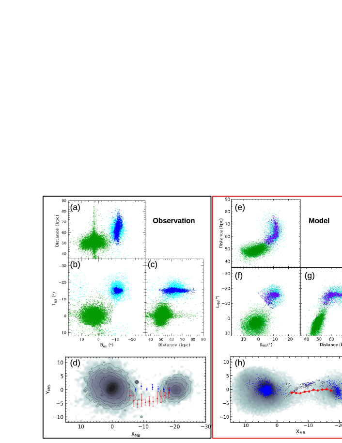
Figure 4: Comparison of the observed stellar distribution (the left panels enclosed within rectangle a black box) of the MCs with that of simulations from Model-52 (the right panels enclosed within a red box). In the observation panels (a, b, c), the observed stars are separated into ancient stars (green for LMC and cyan for SMC) and young stars (blue, age$<$300 Myr). The former are traced by RR Lyrae stars and the latter by classical Cepheids (Ripepi et al., 2017). The top right panels (panels e, f, g, h) particles in ancient stars (green and cyan) are randomly selected to reach the same number as in the observations. In both observations and simulations young stars follow an elongated shape distribution along the line-of-sight, which is well explained by the interaction of the gas from which they formed with the LMC. The bottom-left panel (panel e) shows RR Lyrae stars from Gaia DR2, overlapped with the results from Belokurov et al. (2017): ancient star (red, RR Lyrae) and young stars (blue, main sequence). The bottom-right panel (panel h) shows results from Model-52 (blue points are stars with age $<$ 150 Myr). The offset between the young and ancient stars in the Bridge occurs in both observations and simulations. In the bottom right panel (panel h) the relative velocity of Bridge young stars are shown with vectors, for which the systematic motion of the SMC has been removed. They indicate that young stars are leaving the SMC, which is fully consistent with recent observations (Oey et al., 2018).

The recent collision between the MCs has a strong effect on the SMC, particularly on the young, $\leq$300 Myr stars, which formed from the gas during the most violent phases of interactions. The young stars identified by Classical Cepheids (CCs) with ages less than 300 Myr indeed show a very unusual 3D shape heavily elongated to about 30 kpc along the line of sight (Ripepi et al., 2017). Fig. 4 compares the 3D stellar distributions of the MCs. Simulations shows that the SMC gas is pressurized by LMC gravitational tides, leading to a strongly elongated 3D shape in which star formation is favored. Fig. 4 shows that young, $\leq$300 Myr stars formed during the interaction have shapes with similar elongations along the line-of-sight than that observed. In both simulations and observations, old stars linked to the initial disc and spheroid have a much less elongated distribution.

There are some apparent differences between the model and data in the distribution of stars. In the observation panel (panel a) of Fig. 4, there are RR Lyrae stars with verticle (distance) distribution which is absent in the simulations (panel e). The large majority of these stars are true Galactic RR Lyrae variables along the line of sight, the rest are pulsators with large distance errors (Ripepi et al., 2017). The differences with respect to the morphology traced by young stars (blue points) can be resolved by fine-tuning of the collision parameters between the MCs, e.g., the mass ratio of progenitors, the relative inclination of the SMC disk, and the pericenter distance. The collision affects the disk of LMC too. Sec. 3.4 shows the results of 3 different models with slightly different parameters. Because the parameter space is huge, finely tuning the parameters will further imply optimizing the match between observations and modeling.

3.3 The Magellanic Bridge for gas and stars

The model reproduces well the HI Bridge as shown in Fig.3. Young, intermediate-age and old stars have been identified in the Bridge (Irwin, Demers & Kunkel, 1990; Skowron et al., 2014; Bagheri, Cioni & Napiwotzki, 2013; Noël et al., 2013). Belokurov et al. (2017) has discovered an offset between young main sequence stars and old stars (traced by RR Lyrae from Gaia Data Release 1, DR1) as shown in the bottom left panel of Fig. 4.

In this section we are verifying whether our modeling of the Bridge is consistent with the discovery by Belokurov et al. (2017) that there is an offset between the distribution of young and old star locations in the Bridge. However Belokurov et al. (2017) used Gaia DR1 data, and in the Appendix A we have used a larger sample from Gaia DR2 to select RR Lyrae stars for analyzing the old population in the Bridge. Here we compare the resulting observed distributions of old and young stellar populations with our simulation. In the right panel of Fig.4, simulations also show a similar offset between young and old stars, though less pronounced, between the young and old stars. Thanks to Gaia, proper motions of OB stars in the Wing region of the SMC indicate a systematic peculiar motion away from the SMC of $64{\pm}8$ km/s (Oey et al., 2018; Schmidt et al., 2018). The bottom right panel of Fig. 4 shows a similar trend: young, $<$150 Myr stars (motions indicated by white arrows) are leaving the SMC towards the LMC. Young stars within the -16 $<X_{\rm MS}<$-10 range have a mean velocity of 19 km/s in the simulation, which is around a third of that observed. We also recover the observed fact (Zivick et al., 2019) that Bridge stars are moving faster when they lie closer to the LMC (see increasing arrow sizes).

3.4 Model variance

Table 2: Simulated Magellanic Clouds and Stream properties

		Magellanic Clouds				Magellanic Stream
Model	MCs	Total Mass	Gas mass	Stellar Mass	Gas fraction	HI mass	warm+hot gas
		$10^{9}$M⊙	$10^{9}$M⊙	$10^{9}$M⊙	%	$10^{9}$M⊙	$10^{9}$M⊙
		R$<$3.5kpc	R$<$3.5kpc	R$<$3.5kpc	R$<$3.5kpc	L${}_{\rm MS}<-25$deg	L${}_{\rm MS}<-25$deg
Mod27	LMC	2.88	0.83	2.05	29%	0.5	0.93
	SMC	0.40	0.22	0.18	55%
Mod28	LMC	3.05	0.93	2.12	30%	0.14	0.81
	SMC	1.73	1.30	0.43	75%
Mod52	LMC	2.45	0.83	1.62	34%	0.15	0.94
	SMC	0.81	0.50	0.31	62%

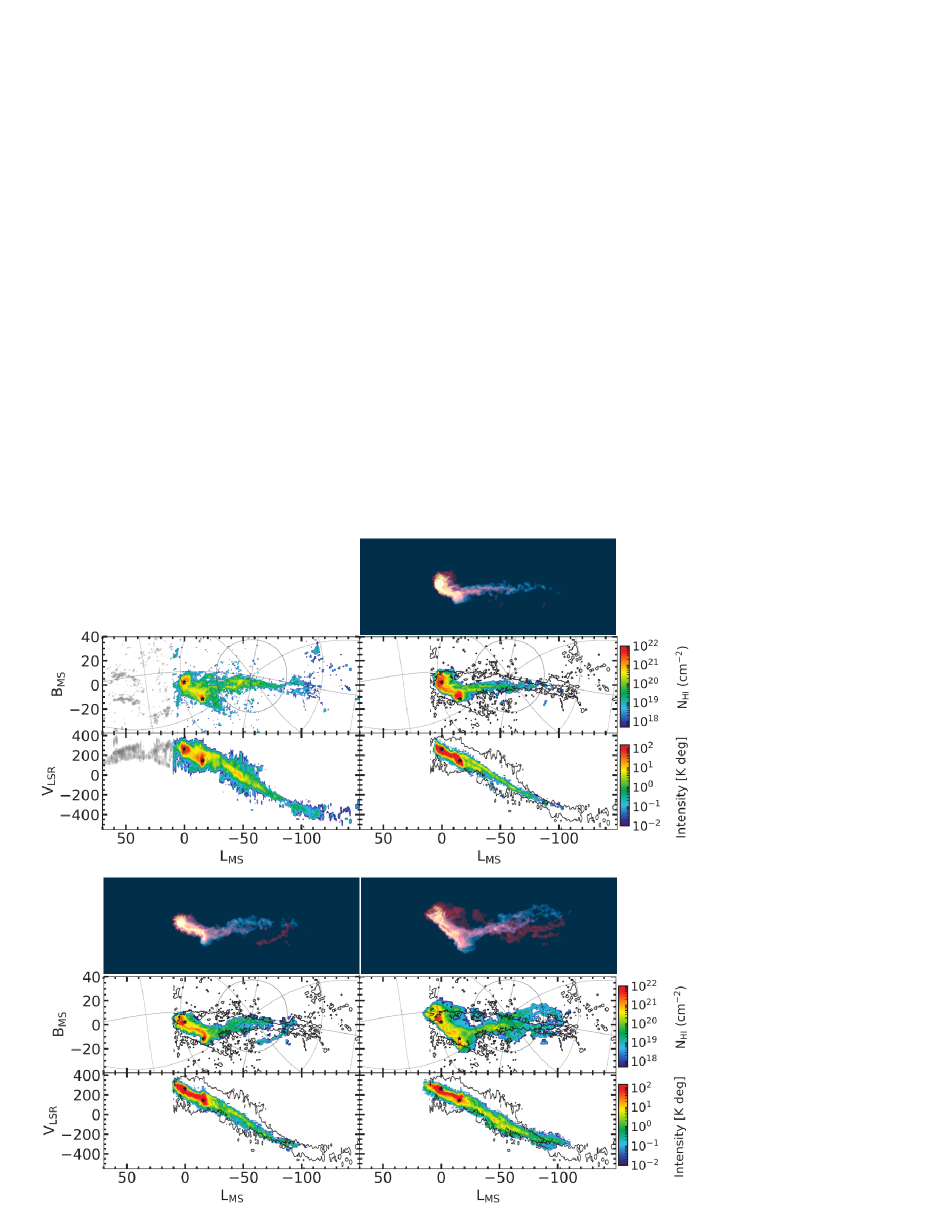
Figure 5: Comparison of three simulated models of Magellanic Stream HI gas distribution with observations (top-left) from Nidever et al. (2010). The simulations refer to Model-28 (top-right), Model-52 (bottom-left), and Model-27 (bottom-right). On the top of each simulation panel, a color image shows the distribution of particles, which have been separated into LMC (red) and SMC (blue) according to their origins.

We have explored a total of $\sim$ 200 different models to compare with observed properties. A comparison between 3 of them is given in Fig. 5, Fig. 6 and Fig. 7 for the HI distribution on the sky, the projected column density distribution, and the 3D star distribution for both MCs. The final results of our models are listed in Table 2.

In Fig. 5 we have distinguished gas particles from LMC and SMC progenitors, which are shown with different colors on the top of each sub-panel of Fig. 5. The MS is composed from both LMC and SMC particles, which form two filaments as observed (Hammer et al., 2015; Nidever et al., 2010). All models reproduce well the main properties, though with some differences.

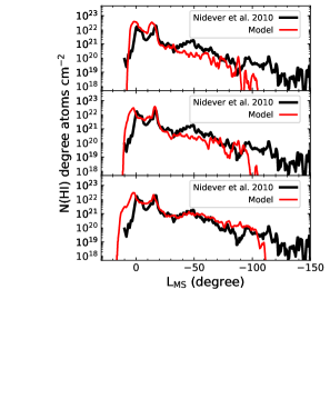
Figure 6: Comparison of the observed HI column density projected along the Magellanic longitude with that provided by three simulation models: Model-28 (top), Model-52 (centre), and Model-27 (bottom). The black line is from observational data (Nidever et al., 2010), and red lines are from simulations.

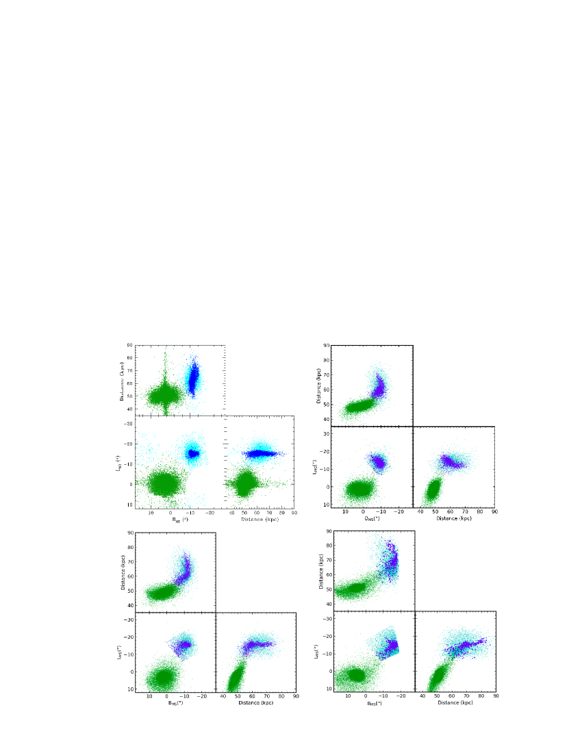
Figure 7: Stellar distribution in 3D for both observations by Ripepi et al. (2017) (top-left panel) and simulations of three models, Model-28 (top-right), Model-52 (bottom-left), and Model-27 (bottom-right). Observed data refer to RR Lyrae for ancient stars (green and cyan), and Classic Cepheids for young stars (blue). In the simulations young stars are selected with having ages lower than 300 Myr. The observing selecting box on the SMC stars (Ripepi et al., 2017) has been applied on the simulation images as it is shown in the sky plane (L_MS, B_MS) sub-panels.

3.5 Limitations of the Modeling

Our model has some weaknesses, linked to the complexity of the problem and to observational uncertainties. The most important one is our choice to model the MW halo gas by a single hot gas component in equilibrium with the MW mass distribution (T $\sim$ $10^{6}K$). Simulations are also not accounting for gas cooling that is metal dependent, or for shielding and UV background. Although ram-pressure depends only on gas-density, a high temperature helps to heat the MS gas, rendering easier the formation of a large ionized gas fraction. It is however likely that the MW halo gas is multi-phased (Lehner et al., 2012; Richter et al., 2017; Prochaska et al., 2017), and this may affect the global balance between ionized and neutral gas in the MS. However uncertainties about the different components of the multi-phase gas in the MW are too large to improve our modeling of the MW halo gas. Moreover, while it is well known (Fox et al., 2014; Richter et al., 2017) that the MS is dominated by the ionized gas, its density along the MS longitude (or distance) is far from being well known, leading to large uncertainties on the total density deposited by the MC, from 1 to 5 $\times 10^{9}$ M_⊙ according to Richter et al. (2017). The above weaknesses are then not affecting the conclusion of the paper : it is the first time the release of more than 50% of the initial gas from the MCs has been modeled.

The series of simulations reproduce all features, but not always at the same time (e.g., for a single model). Of more concern is the fact that a few features are not reproduced by any model. For example, the simulated HI velocity along the Magellanic longitude is not as broad as observed. This could be due to an insufficient account of shocks, or perhaps of contamination by background structures such as HI emission from the Sculptor group. Most other discrepancies (e.g., number of young stars in the Bridge) can be solved by fine tuning orbital parameters or the star formation efficiency.

4 CONCLUSION

The recent infalling of the MCs into the MW gaseous halo and their mutual interaction have formed the gigantic MS and the Bridge, which are fully reproduced by a simulation based on a very precise hydrodynamic solver. This includes detailed properties such as the two filamentary structures of the MS (see Fig.5). Accounting for K-H effects automatically generates large amounts of ionized gas. It is the first time that a physical modeling is able to explain and reproduce the enormous quantities of gas stripped from the MCs, i.e., more than 50% of their initial content. This adds another challenge to the ’tidal’ scenario, which is unable to provide such large gas amounts extracted from a single tidal tail (Pardy, D’Onghia & Fox, 2018; Tepper-García et al., 2019; Diaz & Bekki, 2012). Masses in excess of $10^{11}$ M_⊙ for the LMC are then likely excluded, while we verified that our modeling may accommodate for masses up to 2 $\times 10^{10}$ M_⊙.

Appendix A RR Lyrae star distribution in the intra-cloud region of the Bridge

Due to their typical variability, relatively easy detection and ubiquity, the RR Lyrae variables are important tracers of the old (age$>$10 Gyr) population of the host galaxy. The OGLE group (Udalski et al., 2015; Soszyński et al., 2016) has identified tens of thousands such pulsators in the LMC and SMC, whereas the all sky survey carried out by the Gaia spacecraft (Gaia Collaboration et al., 2016b), presented in DR1 and DR2 (Gaia Collaboration et al., 2016a, 2018a) contributed to the detection of RR Lyrae variables in the outskirt of the MCs and in the intra-cloud region, beyond the OGLE survey footprint (Clementini et al., 2016, 2019).

The Gaia DR1 data were exploited by Belokurov et al. (2017), who found bona fide RR Lyrae candidate variables relying only on the Gaia’s mean flux and its associated errors. On these bases Belokurov et al. (2017) claimed the presence of a second old Bridge between the MCs, not aligned with the gaseous MB, and shifted by $\sim$5 deg from the young main sequence Bridge. Giving the limited information available, the Belokurov et al. (2017)’s RR Lyrae sample completeness and purity are low in comparison with surveys where light curve and colour data are available. This is the case of Gaia DR2 where light curves for $\sim$140K RR Lyrae were published in the Gaia $G$ band and for $\sim$83K also in the $G_{BP}$ and $G_{RP}$ bands. These data, in conjunction with the OGLE dataset, provide a reliable sample of RR Lyrae to study the distribution of old stars around and in-between the MCs. This dataset can be used to update the Belokurov et al. (2017) analysis and the result of this operation is shown in Fig. 4, where to select objects likely belonging to the Magellanic System, we displayed only RR Lyrae with V$>$18 mag (diffuse gray regions). An inspection of the figure reveals that the old Bridge (red symbols) suggested by Belokurov et al. (2017) is substantially confirmed. There are also differences, such as a concentration of objects at ${\rm X}_{\rm MB},{\rm Y}_{\rm MB}$=-11,-2 deg, where the distribution of the pulsators traced by the Gaia DR2 dataset is displaced towards the north by $\sim$2 deg with respect to Belokurov et al. (2017), lying very close to the young main sequence Bridge (blue symbols).

References

- Abadi, Moore & Bower (1999) Abadi M. G., Moore B., Bower R. G., 1999, MNRAS, 308, 947
- Bagheri, Cioni & Napiwotzki (2013) Bagheri G., Cioni M.-R. L., Napiwotzki R., 2013, A&A, 551, A78
- Barger et al. (2017) Barger K. A. et al., 2017, ApJ, 851, 110
- Barnes (2002) Barnes J. E., 2002, MNRAS, 333, 481
- Belokurov et al. (2017) Belokurov V., Erkal D., Deason A. J., Koposov S. E., De Angeli F., Evans D. W., Fraternali F., Mackey D., 2017, MNRAS, 466, 4711
- Besla et al. (2012) Besla G., Kallivayalil N., Hernquist L., van der Marel R. P., Cox T. J., Kereš D., 2012, MNRAS, 421, 2109
- Bhattacharjee, Chaudhury & Kundu (2014) Bhattacharjee P., Chaudhury S., Kundu S., 2014, ApJ, 785, 63
- Bland-Hawthorn et al. (2013) Bland-Hawthorn J., Maloney P. R., Sutherland R. S., Madsen G. J., 2013, ApJ, 778, 58
- Clementini et al. (2016) Clementini G. et al., 2016, A&A, 595, A133
- Clementini et al. (2019) Clementini G. et al., 2019, A&A, 622, A60
- Cox et al. (2006) Cox T. J., Jonsson P., Primack J. R., Somerville R. S., 2006, MNRAS, 373, 1013
- Diaz & Bekki (2012) Diaz J. D., Bekki K., 2012, ApJ, 750, 36
- D’Onghia & Fox (2016) D’Onghia E., Fox A. J., 2016, ARA&A, 54, 363
- Fillingham et al. (2016) Fillingham S. P., Cooper M. C., Pace A. B., Boylan-Kolchin M., Bullock J. S., Garrison-Kimmel S., Wheeler C., 2016, MNRAS, 463, 1916
- For et al. (2014) For B.-Q., Staveley-Smith L., Matthews D., McClure-Griffiths N. M., 2014, ApJ, 792, 43
- Fox et al. (2013) Fox A. J., Richter P., Wakker B. P., Lehner N., Howk J. C., Ben Bekhti N., Bland-Hawthorn J., Lucas S., 2013, ApJ, 772, 110
- Fox et al. (2014) Fox A. J. et al., 2014, ApJ, 787, 147
- Fox et al. (2005) Fox A. J., Wakker B. P., Savage B. D., Tripp T. M., Sembach K. R., Bland-Hawthorn J., 2005, ApJ, 630, 332
- Gaia Collaboration et al. (2018a) Gaia Collaboration et al., 2018a, A&A, 616, A1
- Gaia Collaboration et al. (2016a) Gaia Collaboration et al., 2016a, A&A, 595, A2
- Gaia Collaboration et al. (2018b) Gaia Collaboration et al., 2018b, A&A, 616, A12
- Gaia Collaboration et al. (2016b) Gaia Collaboration et al., 2016b, A&A, 595, A1
- Gunn & Gott (1972) Gunn J. E., Gott, III J. R., 1972, ApJ, 176, 1
- Gupta et al. (2012) Gupta A., Mathur S., Krongold Y., Nicastro F., Galeazzi M., 2012, ApJL, 756, L8
- Hammer et al. (2015) Hammer F., Yang Y. B., Flores H., Puech M., Fouquet S., 2015, ApJ, 813, 110
- Hammer et al. (2018) Hammer F., Yang Y. B., Wang J. L., Ibata R., Flores H., Puech M., 2018, MNRAS, 475, 2754
- Hernquist (1993) Hernquist L., 1993, Survey. ApJ Suppl. Ser., 86, 389
- Hopkins (2015) Hopkins P. F., 2015, MNRAS, 450, 53
- Hopkins (2017) Hopkins P. F., 2017, arXiv:1712.01294
- Huang et al. (2016) Huang Y. et al., 2016, MNRAS, 463, 2623
- Irwin, Demers & Kunkel (1990) Irwin M. J., Demers S., Kunkel W. E., 1990, Astron. J., 99, 191
- Kalberla & Haud (2006) Kalberla P. M. W., Haud U., 2006, A&A, 455, 481
- Kallivayalil et al. (2013) Kallivayalil N., van der Marel R. P., Besla G., Anderson J., Alcock C., 2013, ApJ, 764, 161
- Katz, Weinberg & Hernquist (1996) Katz N., Weinberg D. H., Hernquist L., 1996, ApJS, 105, 19
- Kazantzidis et al. (2017) Kazantzidis S., Mayer L., Callegari S., Dotti M., Moustakas L. A., 2017, ApJL, 836, L13
- Lehner et al. (2012) Lehner N., Howk J. C., Thom C., Fox A. J., Tumlinson J., Tripp T. M., Meiring J. D., 2012, MNRAS, 424, 2896
- Marasco et al. (2015) Marasco A., Debattista V. P., Fraternali F., van der Hulst T., Wadsley J., Quinn T., Roškar R., 2015, MNRAS, 451, 4223
- Mastropietro et al. (2005) Mastropietro C., Moore B., Mayer L., Wadsley J., Stadel J., 2005, MNRAS, 363, 509
- Mathewson, Cleary & Murray (1974) Mathewson D. S., Cleary M. N., Murray J. D., 1974, ApJ, 190, 291
- Miller & Bregman (2013) Miller M. J., Bregman J. N., 2013, ApJ, 770, 118
- Nakashima et al. (2018) Nakashima S., Inoue Y., Yamasaki N., Sofue Y., Kataoka J., Sakai K., 2018, ApJ, 862, 34
- Nidever et al. (2013) Nidever D. L. et al., 2013, in American Astronomical Society Meeting Abstracts, Vol. 221, American Astronomical Society Meeting Abstracts #221, p. 404.04
- Nidever, Majewski & Butler Burton (2008) Nidever D. L., Majewski S. R., Butler Burton W., 2008, ApJ, 679, 432
- Nidever et al. (2010) Nidever D. L., Majewski S. R., Butler Burton W., Nigra L., 2010, ApJ, 723, 1618
- Noël et al. (2013) Noël N. E. D., Conn B. C., Carrera R., Read J. I., Rix H.-W., Dolphin A., 2013, ApJ, 768, 109
- Oey et al. (2018) Oey M. S. et al., 2018, ApJL, 867, L8
- Pardy, D’Onghia & Fox (2018) Pardy S. A., D’Onghia E., Fox A. J., 2018, ApJ, 857, 101
- Prochaska et al. (2017) Prochaska J. X. et al., 2017, ApJ, 837, 169
- Putman, Peek & Joung (2012) Putman M. E., Peek J. E. G., Joung M. R., 2012, ARA&A, 50, 491
- Richter et al. (2013) Richter P., Fox A. J., Wakker B. P., Lehner N., Howk J. C., Bland-Hawthorn J., Ben Bekhti N., Fechner C., 2013, ApJ, 772, 111
- Richter et al. (2017) Richter P. et al., 2017, A&A, 607, A48
- Ripepi et al. (2017) Ripepi V. et al., 2017, MNRAS, 472, 808
- Salem et al. (2015) Salem M., Besla G., Bryan G., Putman M., van der Marel R. P., Tonnesen S., 2015, ApJ, 815, 77
- Schmidt et al. (2018) Schmidt T., Cioni M.-R., Niederhofer F., Diaz J., Matijevic G., 2018, arXiv: 1810.02701
- Skowron et al. (2014) Skowron D. M. et al., 2014, ApJ, 795, 108
- Sofue (2015) Sofue Y., 2015, PASJ, 67, 75
- Sokołowska et al. (2016) Sokołowska A., Mayer L., Babul A., Madau P., Shen S., 2016, ApJ, 819, 21
- Soszyński et al. (2016) Soszyński I. et al., 2016, Acta Astronomica, 66, 131
- Sutherland & Dopita (1993) Sutherland R. S., Dopita M. A., 1993, ApJS, 88, 253
- Tepper-García et al. (2019) Tepper-García T., Bland-Hawthorn J., Pawlowski M. S., Fritz T. K., 2019, arXiv:1901.05636
- Udalski et al. (2015) Udalski A. et al., 2015, Acta Astronomic, 65, 341
- van der Kruit (2007) van der Kruit P. C., 2007, A&A, 466, 883
- Vasiliev (2013) Vasiliev E., 2013, MNRAS, 434, 3174
- Vasiliev & Athanassoula (2015) Vasiliev E., Athanassoula E., 2015, MNRAS, 450, 2842
- Wang et al. (2012) Wang J., Hammer F., Athanassoula E., Puech M., Yang Y., Flores H., 2012, A&A, 538, A121
- Werk et al. (2014) Werk J. K. et al., 2014, ApJ, 792, 8
- Yang & Hammer (2010) Yang Y., Hammer F., 2010, ApJL, 725, L24
- Yang et al. (2014) Yang Y., Hammer F., Fouquet S., Flores H., Puech M., Pawlowski M. S., Kroupa P., 2014, MNRAS, 442, 2419
- Zheng et al. (2019) Zheng Y., Peek J. E. G., Putman M. E., Werk J. K., 2019, ApJ, 871, 35
- Zivick et al. (2019) Zivick P. et al., 2019, ApJ, 874, 78