Thermo-magnetic corrections to $\pi$-$\pi$ Scattering Lengths in the Linear Sigma Model

Abstract

In this article, we extend our previous study of the $\pi$-$\pi$ scattering lengths under the presence of an external magnetic field, including finite temperature effects. The novelty of this work is precisely the introduction of temperature into the discussion, and its interplay with the magnetic field. As in the previous article, we base our analysis in the linear sigma-model, and our calculations are exact within this context. Although the effects are comparatively small, it is interesting to remark that magnetic field and temperature display opposite effects over the scattering lengths.

I Introduction

An interesting and relevant question in the field of heavy ion collision experiments is to search for the possibility of disentangling temperature and magnetic effects. In this article we will refer to $\pi-\pi$ scattering lengths, extending our previous results PRDT0 at zero temperature and finite magnetic fields. In this work, we shall present analytical results that fully capture both thermal and magnetic effects without any restriction or special ordering in these parameters. For this purpose, our calculations will be based on the linear sigma model using techniques associated to the spectral density functions that allows us to handle the infinite series over Landau levels in a closed analytical form. Infinite Matsubara sums were also performed exactly with complex contour integration techniques.

The paper is organized as follows: In section II, we introduce the Linear sigma model and the general formalism for scattering lengths. In section III, the detailed Feynman diagrams are displayed, using the Schwinger propagators for finite magnetic fields. The two master integrals required for the calculation of all the diagrams are formulated. Therein, we also display the analytical results for the scattering lengths, with mathematical details deferred to Appendixes. Finally, in section IV we show our numerical results, discussing the combined effects of temperature and magnetic field.

II Linear sigma model and $\pi$-$\pi$ scattering

In our previous article PRDT0 we studied the $\pi$-$\pi$ scattering lengths within the context of the linear sigma model in the phase where the chiral symmetry is broken,

$$\mathcal{L} = \bar{\psi}\left[i\gamma^{\mu}\partial_{\mu}-m_{\psi}-g(\sigma+i\vec{\pi}\cdot\vec{\tau}\gamma_{5})\right]\psi$$

$$+\frac{1}{2}\left[(\partial\vec{\pi})^{2}+m_{\pi}^{2}\vec{\pi}^{2}\right]+\frac{1}{2}\left[(\partial\sigma)^{2}+m_{\sigma}^{2}\sigma^{2}\right]$$

$$-\lambda^{2}v\sigma(\sigma^{2}+\vec{\pi}^{2})-\frac{\lambda^{2}}{4}(\sigma^{2}+\vec{\pi}^{2})^{2}+(\varepsilon c-vm_{\pi}^{2})\sigma.$$

The model includes a doublet of Fermi fields, which in our case will be ignored since they represent nucleons which are too heavy as compared with the scalar sigma meson and the relevant energy scale. The role of the sigma meson is to break explicitly the chiral symmetry. Then, as usual, the sigma field is expanded around its expectation value and its not difficult to see that $m_{\psi}=gv$, $m_{\pi}^{2}=\mu^{2}+\lambda^{2}v^{2}$ and $m_{\sigma}^{2}=\mu^{2}+3\lambda^{2}v^{2}$. For details see Lee . Perturbation theory at the tree level allows us to identify the pion decay constants as $f_{\pi}=v$. Finite temperature effects on this model have been studied by several authors, discussing the thermal evolution of masses, $f_{\pi}(T)$, the effective potential, etc. cep ; renor ; masa ; super ; magn ; inverse ; sigma ; Loewe ; Larsen ; Bilic ; Petropolus ; wagner ; kovacs1 ; kovacs2 ; kovacs3 .

The most general decomposition for the scattering amplitude for particles with definite isospin quantum numbers is Collins ; Gasser

$$T_{\alpha\beta;\delta\gamma} = A(s,t,u)\delta_{\alpha\beta}\delta_{\delta\gamma}+A(t,s,u)\delta_{\alpha\gamma}\delta_{\beta\delta}$$ (2)

$$+A(u,t,s)\delta_{\alpha\delta}\delta_{\beta\gamma},$$

where $\alpha$, $\beta$, $\gamma$, $\delta$ denote isospin components.

By using appropriate projection operators, it is possible to find the following isospin dependent scattering amplitudes

$$T^{0} =3A(s,t,u)+A(t,s,u)+A(u,t,s),$$ (3)

$$T^{1} =A(t,s,u)-A(u,t,s),$$ (4)

$$T^{2} =A(t,s,u)+A(u,t,s),$$ (5)

where $T^{I}$ denotes a scattering amplitude in a given isospin channel $I=\{0,1,2\}$.

As it is well known Collins , below the inelastic threshold any scattering amplitude can be expanded in terms of partial amplitudes which can be parametrized by the phase shifts for each angular momentum channel $\ell$. Therefore, in the low-energy region the isospin dependent scattering amplitude can be expanded in partial wave components $T_{\ell}^{I}$. The real part of this amplitude

$$\Re\left(T_{\ell}^{I}\right)=\left(\frac{p^{2}}{m_{\pi}^{2}}\right)^{\ell}\left(a_{\ell}^{I}+\frac{p^{2}}{m_{\pi}^{2}}b_{\ell}^{I}+\ldots\right)$$ (6)

is expressed in terms of the scattering lengths $a_{\ell}^{I}$, and the scattering slopes $b_{\ell}^{I}$, respectively. The scattering lengths satisfy the hierarchy $|a_{0}^{I}|>|a_{1}^{I}|>|a_{2}^{I}|...$. In particular, in order to obtain the scattering lengths $a_{0}^{I}$, it is sufficient to calculate the scattering amplitude $T^{I}$ in the static limit, i.e. when $s\to 4m_{\pi}^{2}$, $t\to 0$ and $u\to 0$

$$a_{0}^{I}=\frac{1}{32\pi}T^{I}\left(s\to 4m_{\pi}^{2},t\to 0,u\to 0\right).$$ (7)

The first measurement of $\pi$-$\pi$ scattering lengths was carried on by Rosellet et al.  Rosellet . More recently, these parameters have been measured using pionium atoms in the DIRAC experiment DIRAC and also through the decay of heavy quarkonium states into $\pi$-$\pi$ final states where the so called cusp-effect was found quarkonium . In our recent work PRDT0 , we obtained an exact analytical expression for Eq. (7) for $I=0,2$ in a background magnetic field of arbitrary strength, at zero temperature. In this article, we extend our previous result to include finite temperatures. Therefore, in what follows we shall present the exact expression for the scattering lengths Eq.(7) at arbitrary magnitudes of the external magnetic field and temperature.

III Scattering lengths at finite magnetic field and finite temperature

In a previous work, based on a perturbative treatment of the bosonic Schwinger propagator valid for small magnetic fields, some of us discussed the magnetic dependence of the $\pi$-$\pi$ scattering lengths within the context of the linear sigma model Leandro . We found that this magnetic evolution displays an opposite trend with respect to thermal corrections on the scattering lengths, in agreement with the literature TLSM . At low magnetic field intensities, the scattering lengths in the isospin channel $I=2$ increase, whereas their projection into the channel $I=0$ diminishes, both as functions of the magnetic field. More recently, we extended the analysis in the zero temperature scenario, thus obtaining exact analytical expressions valid in the whole range of magnetic field intensities PRDT0 .

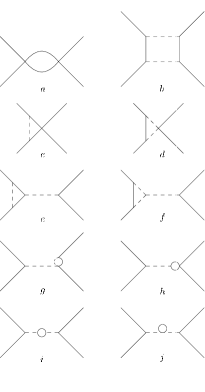
Figure 1: One-loop diagrams relevant to the $\pi$-$\pi$ scattering lengths

. Continuous and dashed lines represent pions and $\sigma$ mesons respectively.

In the linear sigma model, the relevant diagrams that contribute to $\pi$-$\pi$ scattering are shown in Fig. 1. Notice that tadpole-like diagrams associated to mass corrections of the sigma field, do not contribute to the $\pi$-$\pi$ scattering amplitudes, since their imaginary part vanishes. These tadpoles are extremely small in the limit of a very large mass of the sigma field. This approximation is valid since, as we know, $m_{\sigma}\approx 550$ MeV is much larger than the pion mass. Fermions, i.e. nucleons that may interact with pions, are not considered in our discussion. As a consequence, the sigma field propagator is contracted to a point.

(a) $s$-channel diagram.

(b) $t$ and $u$ channel diagram.

Figure 2: “Fish-type” diagrams.

From these considerations, we see that all relevant diagrams reduce to a horizontal ($s$-channel) or vertical ($t$ and $u$ channels) “fish-type” pion loops contributions, as shown in Fig. 2. Then, we need to compute such diagrams as a function of the magnetic field intensity and finite temperature. This is an interesting problem, not only because of physical implications, but also due to new analytical results that we shall present below.

Let us derive our starting expression for the bosonic propagator as a sum of Landau levels Ayalaetal ; PRDT0 . The bosonic Schwinger propagator for a charged pion of charge $q$ subject to a uniform magnetic field along the third spatial coordinate, in the proper time representation is given by

$$iD^{B}(k) =\int_{0}^{\infty}\frac{ds}{\cos(qBs)}e^{is\left(k_{||}^{2}-k_{\perp}^{2}\frac{\tan(qBs)}{qBs}-m_{\pi}^{2}+i\epsilon\right)}.$$ (8)

After inserting this propagator in the fish-type diagrams, one finds that all contributions reduce to two types of integrals PRDT0

$$I_{1}[B,p_{0}] = \int\frac{d^{4}k}{(2\pi)^{4}}iD^{B}(k_{0},\mathbf{k})iD^{B}(k_{0}-2p_{0},\mathbf{k}),$$ (9)

$$I_{2}[B] = \int\frac{d^{4}k}{(2\pi)^{4}}\left[iD^{B}(k_{0},\mathbf{k})\right]^{2}.$$ (10)

For technical purposes, we shall calculate the integrals with the expression for the propagator at finite magnetic field in terms of Landau levels, as presented in Ayalaetal .

$$iD^{B}(k)=2\sum_{l=0}^{\infty}(-1)^{l}L_{l}\left(\frac{2k_{\perp}^{2}}{qB}\right)e^{-k_{\perp}^{2}/qB}i\Delta_{l}^{B}(k_{\parallel}),$$ (11)

where $L_{l}(z)$ are the Laguerre polynomials, and we have defined the effective “parallel” propagators

$$i\Delta_{l}^{B}(k_{\parallel})=\frac{i}{k_{\parallel}^{2}-(2l+1)qB-m_{\pi}^{2}+i\epsilon}.$$ (12)

The above expressions correspond to the zero-temperature scenario. However, it is straightforward to generalize them to the finite temperature case by analytic continuation into Matsubara frequency space, i.e.

$$k_{0}\rightarrow i\omega_{n}=2\pi n/\beta, n\in Z,$$

$$p_{0}\rightarrow i\nu_{m}=2\pi m/\beta, m\in Z$$ (13)

where $\beta=1/T$, and the corresponding substitution of the integral in $k_{0}$ by a sum,

$$\int\frac{d^{2}k_{\parallel}}{(2\pi)^{2}}\rightarrow\frac{i}{\beta}\sum_{n\in Z}\int_{-\infty}^{+\infty}\frac{dk_{3}}{2\pi}$$ (14)

Let us first consider the calculation of $I_{1}[T,B,p_{0}]$, after its definition in Eq.(10), substituting the infinite series for the propagators, Eq.(11), we are lead to

$$I_{1}[T,B,i\nu_{m}]=\frac{i}{\beta}\sum_{n\in Z}\int\frac{d^{3}k}{(2\pi)^{3}}iD^{B}(i\omega_{n},\mathbf{k})$$

$$\times iD^{B}(i\omega_{n}-2i\nu_{m},\mathbf{k})$$

$$=4\sum_{l=0}^{\infty}\sum_{l^{\prime}=0}^{\infty}(-1)^{l+l^{\prime}}G_{l,l^{\prime}}(i\nu_{m})$$

$$\times\left[\int\frac{d^{2}k_{\perp}}{(2\pi)^{2}}e^{-2\,k_{\perp}^{2}/qB}L_{l}\left(\frac{2k_{\perp}^{2}}{qB}\right)L_{l^{\prime}}\left(\frac{2k_{\perp}^{2}}{qB}\right)\right].$$

Here, we have defined the functions

$$G_{l,l^{\prime}}(T,i\nu_{m}) = \int_{-\infty}^{\infty}\frac{dk_{3}}{2\pi}\frac{i}{\beta}\sum_{n\in Z}i\Delta_{l}^{B}(i\omega_{n},k_{3})$$ (16)

$$\times i\Delta_{l^{\prime}}^{B}(i\omega_{n}-2i\nu_{m},k_{3}).$$

Let us now calculate the integral over the Laguerre polynomials in the second term, by using 2-dimensional “spherical coordinates”, with $0\leq|k_{\perp}|<\infty$,

$$d^{2}k_{\perp} = 2\pi|k_{\perp}|d|k_{\perp}|=\frac{\pi\,q\,B}{2}dx,$$ (17)

where we have defined the auxiliary variable $x=2k_{\perp}^{2}/qB$, with $0\leq x<\infty$. Therefore, we have

$$\int\frac{d^{2}k_{\perp}}{(2\pi)^{2}}e^{-2\,k_{\perp}^{2}/qB}L_{l}\left(\frac{2k_{\perp}^{2}}{qB}\right)L_{l^{\prime}}\left(\frac{2k_{\perp}^{2}}{qB}\right)$$ (18)

$$= \frac{1}{4\pi^{2}}\frac{\pi\,qB}{2}\int_{0}^{\infty}dxe^{-x}L_{l}(x)L_{l^{\prime}}(x)$$

$$= \frac{qB}{8\pi}\delta_{l,l^{\prime}},$$

where the orthogonality relation between Laguerre polynomials was used. Substituting this result into Eq.(LABEL:eq_double_sum), we end up with the expression

$$I_{1}[T,B,i\nu_{m}]=\frac{qB}{2\pi}\sum_{l=0}^{\infty}G_{l,l}(T,i\nu_{m}).$$ (19)

As shown in detail in Appendix, we calculate $G_{l,l}(i\nu_{m})$ by first integrating over $k_{0}$ in the complex plane, and later over $k_{3}$. This procedure allows us to obtain the infinite series

$$I_{1}[T,B,i\nu_{m}] = \frac{qB}{4\pi(i\nu_{m})}$$

$$\times \Im m\,\sum_{l=0}^{\infty}\int_{-\infty}^{+\infty}\frac{dk_{3}}{2\pi}g(T,E_{l}(k_{3}),i\nu_{m}),$$

with $E_{l}(k_{3})=\sqrt{k_{3}^{2}+m_{\pi}^{2}+qB(2l+1)}$, and the functions $g(T,E,i\nu_{m})$ defined by

$$g(T,E,i\nu_{m})=\frac{\coth\left(\beta E/2\right)}{E[E-i\nu_{m}]}.$$ (21)

As discussed in Appendix, we introduce the spectral density

$$\rho(E)=\sum_{l=0}^{\infty}\int_{-\infty}^{\infty}\frac{dk_{3}}{2\pi}\delta\left(E-E_{l}(k_{3})\right),$$ (22)

such that Eq.(19) can be expressed as single integral over the energy domain

$$I_{1}[T,B,i\nu_{m}]=\frac{qB}{4\pi(i\nu_{m})}\Im m\,\int_{0}^{\infty}dE\rho(E)g(T,E,i\nu_{m}),$$

where a closed analytical expression for the spectral density was derived in Appendix,

$$\rho(E) = \frac{E}{\pi\sqrt{2qB}}\Theta\left(E-\sqrt{m_{\pi}^{2}+qB}\right)$$ (24)

$$\times\left\{\zeta\left(\frac{1}{2},\frac{E^{2}-m_{\pi}^{2}-qB}{2qB}-\Bigg{\lfloor}\frac{E^{2}-m_{\pi}^{2}-qB}{2qB}\Bigg{\rfloor}\right)\right.$$

$$\left.-\zeta\left(\frac{1}{2},\frac{E^{2}-m_{\pi}^{2}-qB}{2qB}+1\right)\right\},$$

with $\lfloor z\rfloor$ the integer part of $z$ and $\zeta(s,z)$ the Hurwitz Zeta function. In order to obtain the scattering lengths $a_{0}^{I}$, we use the decomposition of the scattering amplitude in the different isospin channels presented in Section II. Since we are only interested in the scattering lengths $a_{0}^{I}$, it is enough to calculate the scattering amplitude in the static limit. Therefore, we normalize by the experimental values at tree level ($a_{0}^{0}(\text{exp})=0.217$ and $a_{0}^{2}(\text{exp})=-0.041$), to obtain the expressions

$$a_{0}^{0}(T,B) = a_{0}^{0}(\text{exp})+\frac{1}{32\pi}\bigl{(}3A(s,t,u)+A(t,s,u)$$

$$+ A(u,t,s)\bigr{)},$$

$$a_{0}^{2}(T,B) = a_{0}^{2}(\text{exp})+\frac{1}{32\pi}\left(A(t,s,u)+A(u,t,s)\right).$$ (25)

Here, $A(s,t,u)$, $A(t,s,u)$ and $A(u,t,s)$ correspond to all $s$-channel, $t$-channel and $u$-channel contributions, respectively. On the other hand, the $s$-channel contribution is obtained from $I_{1}[T,B,i\nu_{m}\rightarrow p_{0}=m_{\pi}]$, while those for the $t$- and $u$-channels are obtained from $I_{2}[T,B]=I_{1}[T,B,i\nu_{m}\rightarrow p_{0}=0]$, according to the following expressions

$$A(s,t,u) = -4\lambda^{4}\left(1-\frac{12\lambda^{2}v^{2}}{m_{\sigma}^{2}}+\frac{24\lambda^{4}v^{4}}{m_{\sigma}^{4}}\right)$$

$$\times I_{1}[T,B,m_{\pi}],$$

$$A(t,s,u)+A(u,t,s) = -8\lambda^{4}\left(1-\frac{12\lambda^{2}v^{2}}{m_{\sigma}^{2}}+\frac{24\lambda^{4}v^{4}}{m_{\sigma}^{4}}\right)$$ (26)

$$\times I_{1}[T,B,0].$$

The experimental values in the absence of magnetic field $B=0$ are given by peyaud $a_{0}^{0}(\text{exp})=0.217$ and $a_{0}^{2}(\text{exp})=-0.041$. The mass for the sigma meson is set to $m_{\sigma}=550$ MeV, and the mass for the pion $m_{\pi}=140$ MeV, with the parameter $v=89$ and $\lambda^{2}=4.26$.

IV Results and Conclusions

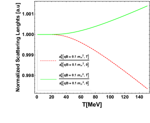
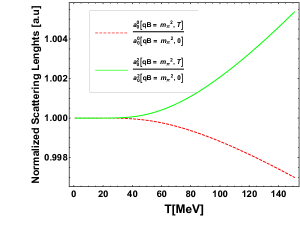
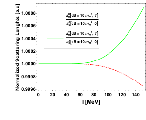
We have presented a novel method to calculate the scattering lengths for $\pi-\pi$ scattering within the linear sigma model at the one-loop level, in the isospin channels $I=\{0,2\}$, as functions of the temperature and external magnetic field intensity. We show three plots of the calculation of the scattering lengths $a_{0}^{0}$ and $a_{0}^{2}$ as a temperature for three magnetic field values. From both figures, it is clear that at finite magnetic field, while $a_{0}^{0}$ increases as a function of temperature, $a_{0}^{2}$ displays the opposite trend. It is interesting to remark that already the presence of a small magnetic field is sufficient to invert the temperature dependence at zero magnetic field TLSM ; Ruiz . This effect can be explained by the symmetry of the scattering length parameters, where $a_{0}^{0}$ arises from the trace of the tensor, which is a scalar, whereas the isospin 2 channel corresponds to the most symmetric realization. Qualitatively, the magnetic moment of the semiclassical orbits associated to the Landau levels tend to align along the magnetic field direction, while temperature tends to randomize those directions. Therefore, under finite magnetic fields the most symmetric state enhances its scattering rate.

Figure 3: (Color online) The scattering parameters $a_{0}^{0}(B,T)/a_{0}^{0}(B,0)$ (dashed) and $a_{0}^{2}(B,T)/a_{0}^{2}(B,0)$ (solid) are displayed as a function of the temperature for $qB=0.1m_{\pi}^{2}$.

Figure 4: (Color online) The scattering parameters $a_{0}^{0}(B,T)/a_{0}^{0}(B,0)$ (dashed) and $a_{0}^{2}(B,T)/a_{0}^{2}(B,0)$ (solid) are displayed as a function of the temperature for $qB=m_{\pi}^{2}$.

Figure 5: (Color online) The scattering parameters $a_{0}^{0}(B,T)/a_{0}^{0}(B,0)$ (dashed) and $a_{0}^{2}(B,T)/a_{0}^{2}(B,0)$ (solid) are displayed as a function of the temperature for $qB=10m_{\pi}^{2}$.

Appendix A Matsubara sums and integrals over $k_{3}$

Here we present in detail the calculation of the Matsubara sums involved in Eq.(19) of the main text. Using the definition of the “parallel” propagators Eq.(12), we have

$$G_{l,l}(T,i\nu_{m}) = \int\frac{dk_{3}}{2\pi}\frac{i}{\beta}\sum_{n\in Z}i\Delta_{l}^{B}(i\omega_{n},k_{3})$$ (27)

$$\times \i\Delta_{l}^{B}(i\omega_{n}-2i\nu_{m},k_{3})$$

$$= i\frac{i^{2}}{2\pi}\int_{-\infty}^{+\infty}dk_{3}f(T,E_{l}(k_{3}),i\nu_{m})$$

where we have defined the expression

$$f(T,E_{l}(k_{3}),i\nu_{m})=\frac{1}{\beta}\sum_{n\in Z}\frac{1}{A(i\omega_{n},k_{3})C(i\omega_{n},k_{3})},$$

(28)

with

$$A(i\omega_{n},k_{3}) = (i\omega_{n})^{2}-E_{l}(k_{3})^{2}+i\epsilon,$$

$$C(i\omega_{n},k_{3}) = (i\omega_{n}-2i\nu_{m})^{2}-E_{l}(k_{3})^{2}+i\epsilon,$$ (29)

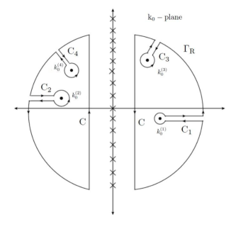
and $E_{l}(k_{3})=\sqrt{k_{3}^{2}+m_{\pi}^{2}+qB(2l+1)}$. The Matsubara sum can be evaluated, as usual, by constructing a contour integral on the complex $k_{0}$-plane,

$$\oint_{C\oplus C_{1}\oplus C_{2}\oplus C_{3}\oplus C_{4}}dk_{0}\frac{n_{B}(k_{0})}{A(k_{0},k_{3})C(k_{0},k_{3})}$$ (30)

where the contour is depicted in Fig.(6). Here, the integrand contains as a factor the Bose-Einstein distribution,

$$n_{B}(k_{0})=\left(\exp(\beta k_{0})-1\right)^{-1}$$ (31)

that possesses infinitely-many simple poles at the Matsubara frequencies $k_{0}=i\omega_{n}=i2\pi n/\beta$, with residue

$$\lim_{k_{0}\rightarrow i\omega_{n}}\frac{k_{0}-i\omega_{n}}{e^{i\omega_{n}}\exp(\beta(k_{0}-i\omega_{n}))-1}=\frac{1}{\beta}.$$ (32)

In addition, the integrand in Eq.(30) possesses four simple poles at $k_{0}^{(1,2)}=\pm E_{l}(k_{3})\mp i\epsilon^{\prime}$ and $k_{0}^{(3,4)}=2i\nu_{m}\pm E_{l}(k_{3})\mp i\epsilon^{\prime}$, i.e., two of them located on the positive imaginary plane, while the other two are located on the negative imaginary plane. By direct application of the residue theorem, we have

$$\oint dk_{0}\frac{n_{B}(k_{0})}{A(k_{0},k_{3})C(k_{0},k_{3})}=0=2\pi i\left(\sum_{j=1}^{4}n_{B}(k_{0}^{(j)})\lim_{k_{0}\rightarrow k_{0}^{(j)}}\frac{(k_{0}-k_{0}^{(j)})}{A(k_{0},k_{3})C(k_{0},k_{3})}+\frac{1}{\beta}\sum_{n\in Z}\frac{1}{A(i\omega_{n},k_{3})C(i\omega_{n},k_{3})}\right).$$ (33)

Clearly, the second term within the parenthesis is precisely the function $f_{l}(T,k_{3},i\nu_{m})$ defined in Eq.(28), and hence we have

$$f(T,E_{l}(k_{3}),i\nu_{m})=-\sum_{j=1}^{4}n_{B}(k_{0}^{(j)})$$

$$\times \lim_{k_{0}\rightarrow k_{0}^{(j)}}\frac{(k_{0}-k_{0}^{(j)})}{A(k_{0},k_{3})C(k_{0},k_{3})}$$

$$= \frac{\left[n_{B}(E_{l}(k_{3}))-n_{B}(-E_{l}(k_{3}))\right]}{4i\nu_{m}E_{l}(k_{3})}$$

$$\times \left\{\frac{1}{2E_{l}(k_{3})-2i\nu_{m}}-\frac{1}{2E_{l}(k_{3})+2i\nu_{m}}\right\},$$

where we used the elementary property of the Bose distribution $n_{B}(z+i\nu_{m})=n_{B}(z)$. Moreover, we also have $n_{B}(-z)=-1-n_{B}(z)$. Therefore, $n_{B}(E_{l}(k_{3}))-n_{B}(-E_{l}(k_{3})=2n_{B}(E_{l}(k_{3}))+1=\coth(\beta E_{l}(k_{3})/2)$, and we finally obtain

$$f(T,E_{l}(k_{3}),i\nu_{m}) =\frac{\coth\left(\beta E_{l}(k_{3})/2\right)}{8i\nu_{m}E_{l}(k_{3})}$$

$$\times\left\{\frac{1}{E_{l}(k_{3})-i\nu_{m}}-\frac{1}{E_{l}(k_{3})+i\nu_{m}}\right\}.$$ (35)

Let us define the functions

$$g(T,E,i\nu_{m})=\frac{\coth\left(\beta E/2\right)}{E[E-i\nu_{m}]},$$ (36)

such that

$$f(T,E_{l}(k_{3}),i\nu_{m}) = \frac{1}{8i\nu_{m}}\bigl{[}g(T,E_{l}(k_{3}),i\nu_{m})$$ (37)

$$- g(T,E_{l}(k_{3}),-i\nu_{m})\bigr{]}.$$

Now we calculate the integral over $k_{3}$. Inserting Eq.(LABEL:eq_f) into Eq.(27), we have

$$G_{l,l}(T,i\nu_{m}) = -\frac{i}{8i\nu_{m}}\int_{-\infty}^{\infty}\frac{dk_{3}}{2\pi}\left(g(T,E_{l}(k_{3}),i\nu_{m})\right.$$

$$\left.-g(T,E_{l}(k_{3}),-i\nu_{m})\right)$$

$$= \frac{1}{4i\nu_{m}}\Im m\,\int_{-\infty}^{\infty}\frac{dk_{3}}{2\pi}g(T,E_{l}(k_{3}),i\nu_{m}).$$

Figure 6: Integration contour in the complex $k_{0}$-plane

.

Appendix B Spectral density

As defined in the main text, here we present the analytical calculation for the spectral density $\rho(E)$. By definition, we have

$$\rho(E)=\sum_{l=0}^{\infty}\int_{-\infty}^{\infty}\frac{dk_{3}}{2\pi}\delta(E-E_{l}(k_{3})).$$ (39)

The condition enforced by the argument of the delta function possesses two algebraic solutions, i.e. $k_{3}=\pm\sqrt{E^{2}-m_{\pi}^{2}-qB(2l+1)}$, but only the positive one possesses support under the integration domain,

$$\delta(E-E_{l}(k_{3}))=\frac{E}{|k_{3}|}\left[\delta\left(k_{3}+\sqrt{E^{2}-m_{\pi}^{2}-qB(2l+1)}\right)\right.$$

$$\left.+\delta\left(k_{3}-\sqrt{E^{2}-m_{\pi}^{2}-qB(2l+1)}\right)\right].$$

By carrying out the integration explicitly, we obtain the expression

$$\rho(E)=\frac{E}{\pi}\sum_{l=0}^{\infty}\frac{\Theta\left(E-\sqrt{m_{\pi}^{2}+qB(2l+1)}\right)}{\sqrt{E^{2}-m_{\pi}^{2}-qB(2l+1)}}.$$ (41)

The infinite sum can be calculated, after noticing that the Heaviside step function restricts the upper limit of the Landau level $0\leq l\leq l_{max}(E)$ for each given value of the energy, through the condition,

$$l_{max}(E)=\Bigg{\lfloor}\frac{E^{2}-m_{\pi}^{2}-qB}{2qB}\Bigg{\rfloor},$$ (42)

with $\lfloor z\rfloor$ the integer part of $z$. Therefore, from this definition, the analytical expression for the spectral density becomes

$$\rho(E) = \frac{E}{\pi\sqrt{2qB}}\Theta\left(E-\sqrt{m_{\pi}^{2}+qB}\right)$$ (43)

$$\times\sum_{l=0}^{l_{max}(E)}\frac{1}{\sqrt{\frac{E^{2}-m_{\pi}^{2}-qB}{2qB}-l}}.$$

It is now convenient to organize the finite sum differently, by defining $\bar{l}=l_{max}(E)-l$. Clearly, we have $0\leq\bar{l}\leq l_{max}(E)$. Therefore, the expression above can be written in the equivalent form

$$\rho(E) = \frac{E}{\pi\sqrt{2qB}}\Theta\left(E-\sqrt{m_{\pi}^{2}+qB}\right)$$ (44)

$$\times\sum_{\bar{l}=0}^{l_{max}(E)}\frac{1}{\sqrt{\frac{E^{2}-m_{\pi}^{2}-qB}{2qB}-l_{max}(E)+\bar{l}}}.$$

By applying the identity that follows from the definition of the Hurwitz Zeta function, for $n\in\mathbb{N}_{0}$,

$$\sum_{l=0}^{n}\frac{1}{\left(z+l\right)^{s}}=\zeta(s,z)-\zeta(s,z+n+1),$$ (45)

we can reduce the density of states to the analytical expression

$$\rho(E) = \frac{E}{\pi\sqrt{2qB}}\Theta\left(E-\sqrt{m_{\pi}^{2}+qB}\right)$$ (46)

$$\times\left\{\zeta\left(\frac{1}{2},\frac{E^{2}-m_{\pi}^{2}-qB}{2qB}-l_{max}(E)\right)\right.$$

$$\left.-\zeta\left(\frac{1}{2},\frac{E^{2}-m_{\pi}^{2}-qB}{2qB}+1\right)\right\}.$$

References

(1) M. Loewe, L. Monje, E. Muñoz, A. Raya and R. Zamora, Phys. Rev. D 99, 056002 (2019).
(2)
B. Lee, “Chiral Dynamics”, Gordon and Breach, 1972.
(3)
A. Ayala, M. Loewe, L. A. Hernandez, J. C. Rojas and R. Zamora, arXiv:1904.11905 [hep-ph].
(4)
M. Correa, M. Loewe, D. Valenzuela and R. Zamora, arXiv:1901.06426 [hep-ph].
(5)
A. Ayala, R. L. S. Farias, S. Ortiz, L. A. Hernandez, D. Manreza Paret and R. Zamora, Phys. Rev. D 98, 114008 (2018).
(6) A. Ayala, M. Hentschinski, L. A. Hernandez, M. Loewe, R. Zamora, Phys. Rev. D 98, 114002 (2018).
(7) A. Ayala, C. A. Dominguez, L. A. Hernandez, M. Loewe and R. Zamora, Phys. Rev. D 92, 096011 (2015).
(8)A. Ayala, M. Loewe and R. Zamora, Phys. Rev. D 91, 016002 (2015).
(9) M. Loewe, C. Villavicencio and R. Zamora, Phys. Rev. D 89, 016004 (2014).
(10)
C. Contreras and M. Loewe, Int. Jour. of Mod. Phys. A5, 2297 (1990).
(11)
A. Larsen, Z. Phys. C 33, 291 (1986).
(12)
N. Bilic and H.Nikolic, Eur. Phys. J. C6, 513 (1999).
(13)
H. Mao, N. Petropoulos and W-K. Zhao, J. Phys. G32, 2187 (2006); N. Petropoulos, arXiv: hep-ph/0402136 and references
therein.
(14)
B. J. Schaefer and M. Wagner, Phys. Rev. D79, 014018 (2009).
(15)
P. Kovacs and Z. Szep, Phys. Rev. D77, 065016 (2008).
(16)
P. Kovacs and Z. Szep, Phys. Rev. D75, 025015 (2007).
(17)
P. Kovacs and Z. Szep, Phys. Rev. D93, 114014 (2016).
(18)
J. Gasser, H. Leutwyler, “Chiral Perturbation Theory to one loop”, Ann. of Physics 158, 142 (1984).
(19)
P. D. B. Collins, “An Introduction to Regge Theory on High Energy Physics”, Cambridge University Press, (1977).
(20)
L. Rosellet, et al. Phys. Rev. D15, 574 (1977).
(21) B. Adeva et al. Phys. Lett. B 701, 24 (2011).