The Effect of Network Width on Stochastic Gradient Descent
and Generalization: an Empirical Study
Supplementary Material
Abstract
We investigate how the final parameters found by stochastic gradient descent are influenced by over-parameterization. We generate families of models by increasing the number of channels in a base network, and then perform a large hyper-parameter search to study how the test error depends on learning rate, batch size, and network width. We find that the optimal SGD hyper-parameters are determined by a “normalized noise scale,” which is a function of the batch size, learning rate, and initialization conditions. In the absence of batch normalization, the optimal normalized noise scale is directly proportional to width. Wider networks, with their higher optimal noise scale, also achieve higher test accuracy. These observations hold for MLPs, ConvNets, and ResNets, and for two different parameterization schemes (“Standard” and “NTK”). We observe a similar trend with batch normalization for ResNets. Surprisingly, since the largest stable learning rate is bounded, the largest batch size consistent with the optimal normalized noise scale decreases as the width increases.
1 Introduction
Generalization is a fundamental concept in machine learning, but it remains poorly understood (Zhang et al., 2016). Theoretical generalization bounds are usually too loose for practical tasks (Harvey et al., 2017; Neyshabur et al., 2017; Bartlett et al., 2017; Dziugaite & Roy, 2017; Zhou et al., 2018; Nagarajan & Kolter, 2018), and practical approaches to hyper-parameter optimization are often developed in an ad-hoc fashion (Sculley et al., 2018). A number of authors have observed that Stochastic Gradient Descent (SGD) can be a surprisingly effective regularizer (Keskar et al., 2016; Wilson et al., 2017; Sagun et al., 2017; Mandt et al., 2017; Smith & Le, 2017; Chaudhari & Soatto, 2017; Soudry et al., 2018). In this paper, we provide a rigorous empirical study of the relationship between generalization and SGD, which focuses on how both the optimal SGD hyper-parameters and the final test accuracy depend on the network width.
This is a broad topic, so we restrict the scope of our investigation to ensure we can collect thorough and unambiguous experimental results within a reasonable (though still substantial) compute budget. We consider training a variety of neural networks on classification tasks using SGD without learning rate decay (“constant SGD”), both with and without batch normalization (Ioffe & Szegedy, 2015). We define the performance of a network by its average test accuracy at “late times” and over multiple training runs. The set of optimal hyperparameters denote the hyper-parameters for which this average test accuracy was maximized. We stress that optimality is defined purely in terms of the performance of the trained network on the test set. This should be distinguished from references to ideal learning rates in the literature, which are often defined as the learning rate which converges fastest during training (LeCun et al., 1996; Karakida et al., 2017). Our use of optimality should also not be confused with references to optimality or criticality in some recent studies (Shallue et al., 2018; McCandlish et al., 2018) where these terms are defined with respect to efficiency of training, rather than final performance.
Given these definitions, we study the optimal hyper-parameters and final test accuracy of networks in the same class but with different widths. Two networks are in the same class if one can be obtained from the other by adjusting the numbers of channels. For example, all three-layer perceptrons are in the same class, while a two-layer perceptron is in a different class to a three-layer perceptron. For simplicity, we consider a “linear family” of networks,
| (1) |
each of which is obtained from a base network by introducing a widening factor, much in the spirit of wide residual networks (Zagoruyko & Komodakis, 2016). That is, network can be obtained from by widening every layer by a constant factor of . We aim to identify a predictive relationship between the optimal hyper-parameters and the widening factor . We also seek to understand the relationship between network width and final test accuracy.
We will find that a crucial factor governing both relationships is the “normalized noise scale”. As observed in (Mandt et al., 2017; Chaudhari & Soatto, 2017; Jastrzebski et al., 2017; Smith & Le, 2017), and reviewed in section 2.2, when the learning rate is sufficiently small, the behaviour of SGD is determined by the noise scale , where for SGD,
| (2) |
and for SGD with momentum,
| (3) |
Here, is the learning rate, is the batch size, is the momentum coefficient, and is the size of the training set. Smith & Le (2017) showed that there is an optimal noise scale , and that any setting of the hyper-parameters satisfying will achieve optimal performance at late times, so long as the effective learning rate is sufficiently small. We provide additional empirical evidence for this claim in section 4. However in this work we argue that to properly define the noise introduced by SGD, should be divided by the square of a weight scale. A quick way to motivate this is through dimensional analysis. In a single SGD step, the parameter update is proportional to the learning rate multiplied by the gradient. Assigning the parameters units of , and the loss units of , the gradient has units of . This implies that the learning rate has dimensions of . The scale of the loss is controlled by the choice of cost function and the dataset. However the weight scale can vary substantially over different models in the same class. We hypothesize that this weight scale is controlled by the scale of the weights at initialization, and it will therefore depend on the choice of parameterization scheme (Jacot et al., 2018). Since the noise scale is proportional to the learning rate, we should therefore divide it by the square of this weight scale.
In this work we will consider two parameterization schemes, both defined in section 2.1. In the “standard” scheme most commonly used in deep learning, the weights are initialized from an isotropic Gaussian distribution whose standard deviation is inversely proportional to the square root of the network width. As detailed above, this work will consider families of networks obtained by multiplying the width of every hidden layer in some base network by a multiplicative factor . Thus the normalized noise scale,
| (4) |
The standard deviation defines the weight scale of the base network, which for our purposes is just a constant. An alternative parameterization was recently proposed, commonly referred to as “Neural Tangent Kernel” parameterization, or “NTK” (van Laarhoven, 2017; Karras et al., 2017; Jacot et al., 2018; Karras et al., 2018). In this scheme, the weights are initialized from a Gaussian distribution whose standard deviation is constant, while the pre-activations are multiplied by the initialization factor (Glorot & Bengio, 2010; He et al., 2015) after applying the weights to the activations in the previous layer. Since the weight scale in this scheme is independent of the widening factor,
| (5) |
By finding the optimal normalized noise scale for families of wide residual networks (WRNs), convolutional networks (CNNs) and multi-layer perceptrons (MLPs) for image classification tasks on CIFAR-10 (Krizhevsky, 2009), Fashion-MNIST (F-MNIST) (Xiao et al., 2017) and MNIST (LeCun et al., 2010), we are able to make the following observations:
-
1.
Without batch normalization, the optimal normalized noise is proportional to the widening factor. That is,
(6) See section 4 for plots. This result implies,
-
•
For the standard scheme, the optimal value of stays constant with respect to the widening factor.
-
•
For the NTK scheme, the optimal value of is proportional to the widening factor.
-
•
-
2.
The definition of the noise scale does not apply to networks with batch normalization, since the gradients of individual examples depend on the rest of the batch. However we have observed that the trend expressed in equation 6 still holds in a weaker sense. Considering networks parameterized using the NTK scheme,
-
•
When the batch size is fixed, the optimal learning rate increases with the widening factor.
-
•
When the learning rate is fixed, the optimal batch size decreases with the widening factor.
-
•
Residual networks (He et al., 2016) obey the trend implied by equation 6 both with and without batch normalization. Furthermore for all networks, both with and without batch normalization, wider networks consistently perform better on the test set (Neyshabur et al., 2018; Lee et al., 2018).
The largest stable learning rate is proportional to in the standard scheme, while it is constant for the NTK scheme (discussed further in section 2.1). This implies that the largest batch size consistent with equation 6 decreases as the network width rises. Since the batch size cannot be smaller than one, these bounds imply that there is a critical network width above which equation 6 cannot be satisfied.
2 Background
2.1 Standard vs. NTK Parameterization Schemes
In the standard scheme, the pre-activations of layer are related to the activations of layer by
| (7) |
and weights and biases are initialized according to
| (8) |
The scalar denotes the input dimension of the weight matrix, and is a common weight scale shared across all models in the same class. For fully connected layers is the dimension of the input, while for convolutional layers is the filter size multiplied by the number of input channels. By inspecting equation 8, we can see that the weight scale is inversely proportional to the square root of the widening factor . Following the discussion in the introduction, we arrive at equation 4 by normalizing the learning rate accordingly:
| (9) |
Meanwhile in the NTK scheme (van Laarhoven, 2017; Jacot et al., 2018), the pre-activations are related to the activations of the previous layer by,
| (10) |
and weights and biases are initialized according to
| (11) |
Notice that the scaling factor is introduced after applying the weights, while the parameter controls the effect of bias. We set in all experiments. The weight scale is independent of the widening factor , leading to a normalized learning rate which also does not depend on ,
| (12) |
We therefore arrive at the normalized noise scale of equation 5. The test set performance of NTK and standard networks are compared in section I of the supplemental material.
The learning rate has an upper-bound defined by convergence criteria and numerical stability. This upper-bound will also be on the order of the square of the weight scale, which implies that the upper-bound for is approximately constant with respect to the widening factor. It follows that the stability bound for the bare learning rate scales like for the standard scheme (Karakida et al., 2017), while it remains constant for the NTK scheme. We provide empirical evidence supporting these stability bounds in section H of the supplementary material. A major advantage of the NTK parameterization is that we can fix a single learning rate and use it to train an entire family of networks without encountering numerical instabilities. We therefore run the bulk of our experiments using the NTK scheme.
2.2 Noise in SGD
Smith & Le (2017) showed that for SGD and SGD with momentum, if the effective learning rate is sufficiently small the dynamics of SGD are controlled solely by the noise scale (equations 2 and 3). This implies that the set of hyperparameters for which the network achieves maximal performance at “late times” is well approximated by a level set of (i.e., the set of hyperparameters for which ). We define “late times” to mean sufficiently long for the validation accuracy to equilibrate. To verify this claim, in our experiments we will make two independent measurements of . One is obtained by holding the learning rate fixed and sweeping over the batch size, while the other is obtained by holding the batch size fixed and sweeping over the learning rate. We find that these two measures of agree closely, and they obtain the same optimal test performance. We refer the reader to section 3.2 for further discussion of training time, and section G of the supplementary material for experiments comparing the test set performance of an MLP across a two dimensional grid of learning rates and batch sizes.
This analysis breaks down when the learning rate is too large (Yaida, 2018). However empirically for typical batch sizes (e.g., on ImageNet), the optimal learning rate which maximizes the test set accuracy is within the range where the noise scale holds111i.e., linear scaling of and does not degrade performance. (Goyal et al., 2017; Smith et al., 2017; McCandlish et al., 2018; Shallue et al., 2018). Our experiments will demonstrate that this does not contradict the common observation that, at fixed batch size, the test set accuracy drops rapidly above the optimal learning rate.
When a network is trained with batch normalization, the gradients for individual samples depend on the rest of the batch, breaking the analysis of Smith & Le (2017). Batch normalization also changes the gradient scale. We therefore do not expect equation 6 to hold when batch normalization is introduced. However we note that at fixed batch size, the SGD noise scale is still proportional to the learning rate.
3 Experiments
3.1 Overview
We run experiments by taking a linear family of networks, and finding the optimal normalized noise scale for each network on a given task. We measure the optimal noise scale in two independent ways—we either fix the learning rate and vary the batch size, or fix the batch size and vary the learning rate. We use fixed Nesterov momentum .
We first describe our experiments at fixed learning rate. We train 20 randomly initialized networks for each model in the family at a range of batch sizes, and compute the test accuracy after training “sufficiently long” (section 3.2). We then compute the average trained network performance and find the batch size with the best average performance . The “trained performance” refers to the average test accuracy of “trained runs” (runs whose final test accuracy exceeds ). We compute the standard deviation of the trained accuracy at this batch size and find all contiguous batch sizes to whose average accuracy is above , where is the number of trained runs at batch size . This procedure selects all batch sizes whose average accuracy is within two standard error deviations of , and it defines the “best batch size interval” , from which we compute the “best normalized noise scale interval” . We estimate the optimal normalized noise scale by . When , we include an error bar to indicate the range. The procedure for computing the optimal normalized noise scale in experiments with fixed batch size is analogous to the procedure above; we train all networks 20 times for a range of learning rates and compute the best learning rate interval .
Our main result is obtained by plotting the optimal normalized noise scale against the widening factor (in the absence of batch normalization). When batch normalization is introduced, the definition of the noise scale is not valid. In this case, we simply report the optimal inverse batch size (learning rate) observed when fixing the learning rate (batch size), respectively. To make the plots comparable, we rerun the estimation procedure used for finding the optimal value of when estimating the optimal value of (batch size search) and (learning rate search).
3.2 Training Time
To probe the asymptotic “late time” behaviour of SGD, we run our experiments with a very large compute budget, where we enforce a lower bound on the training time both in terms of the number of training epochs and the number of parameter updates. When we run learning rate searches with fixed batch size, we take a reference learning rate, for which the training steps are computed based on the epoch/step constraints, and then scale this reference training time accordingly for different learning rates. Although we find consistent relationships between the batch size, learning rate, and test error, it is still possible that our experiments are not probing asymptotic behavior (Shallue et al., 2018).
We terminate early any training run whose test accuracy falls below at any time beyond of the total training time . We verified that at least 15 training runs completed successfully for each experiment (learning rate/batch size pair). See sections B and C of the supplementary material for a detailed description of the procedure used to set training steps and impose lower bounds on training time.
3.3 Networks and Datasets
We consider three classes of networks; multi-layer perceptrons, convolutional neural networks and residual networks. We use ReLU nonlinearities in all networks, with softmax readout. The weights are initialized at criticality with (He et al., 2015; Schoenholz et al., 2016).
We perform experiments on MLPs, CNNs and ResNets. We consider MLPs with 1, 2 or 3 hidden layers and denote the -layered perceptron with uniform width by the label . Our family of convolutional networks is obtained from the celebrated LeNet-5 (figure 2 of Lecun et al. (1998)) by scaling all the channels, as well as the fully connected layers, by a widening factor of . Our family of residual networks is obtained from table 1 of Zagoruyko & Komodakis (2016) by taking and . Batch normalization is only explored for CNNs and WRNs.
We train these networks for classification tasks on MNIST, Fashion-MNIST (F-MNIST), and CIFAR-10. More details about the networks and datasets used in the experiments can be found in section A of the supplementary material.
We train with a constant learning rate, and do not consider data augmentation, weight decay or other regularizers in the main text. Learning rate schedules and regularizers introduce additional hyper-parameters which would need to be tuned for every network width, minibatch size, and learning rate. This would have been impractical given our computational resources. However we selected a subset of common regularizers (label smoothing, data augmentation and dropout) and ran batch size search experiments for training WRNs on CIFAR-10 in the standard parameterization with commonly used hyper-parameter values. We found that equation 6 still held in these experiments, and increasing network width improved the test accuracy. These results can be found in section F of the supplementary material.
 |
 |
 |
 |
 |
 |
 |
 |
 |
 |
 |
 |
 |
 |
 |
 |
 |
 |
 |
 |
4 Experiment Results
Most of our experiments are run with networks parameterized in the NTK scheme without batch normalization. These experiments, described in section 4.1, provide the strongest evidence for our main result, (equation 6). We independently optimize both the batch size at constant learning rate and the learning rate at constant batch size, and confirm that both procedures predict the same optimal normalized noise scale and achieve the same test accuracy.
We have conducted experiments on select dataset-network pairs with standard parameterization and without batch normalization in section 4.2. In this section we only perform batch size search at fixed learning rate. Finally we run experiments on NTK parameterized WRN and CNN networks with batch normalization in section 4.3, for which we perform both batch size search and learning rate search. Some additional batch size search experiments for WRNs parameterized in the standard scheme with batch normalization can be found in section E of the supplementary material, while we provide an empirical comparison of the test performance of standard and NTK parameterized networks in section I. We provide a limited set of experiments with additional regularization in section F of the supplementary material.
In section 4.4, we study how the final test accuracy depends on the network width and the normalized noise scale.
4.1 NTK without Batch Normalization
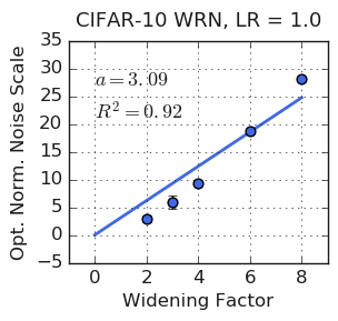
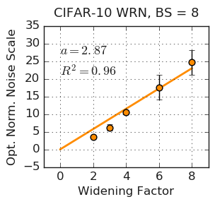
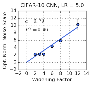
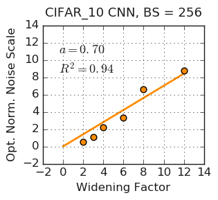
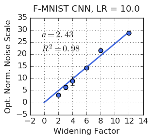
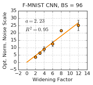
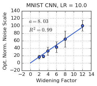
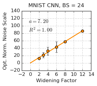
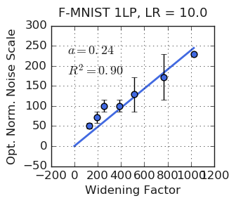
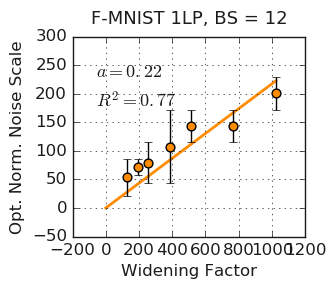
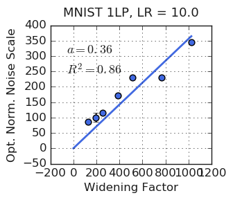
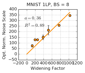
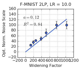
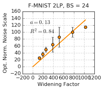
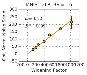
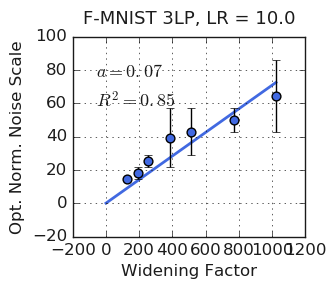
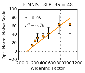
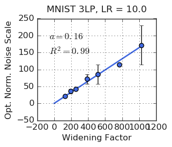
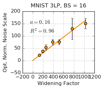
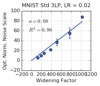
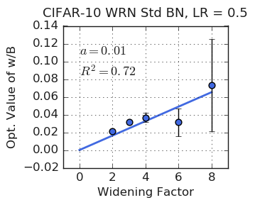
In figure 1, we plot the optimal normalized noise scale against the widening factor for a wide range of network families. The blue plots were obtained by batch size search with fixed learning rate, while the orange plots were obtained by learning rate search with fixed batch size. The fixed batch size or learning rate is given in the title of each plot alongside the dataset and network family. As explained in section 3.1, the error bars indicate the range of normalized noise scales that yield average test accuracy within the % confidence interval of the best average test accuracy. For each plot we fit the proportionality constant to the equation , and provide both and the value. We observe a good fit in each plot. The proportionality constant is computed independently for each dataset-network family pair by both batch size search and learning rate search, and these two constants consistently agree well.
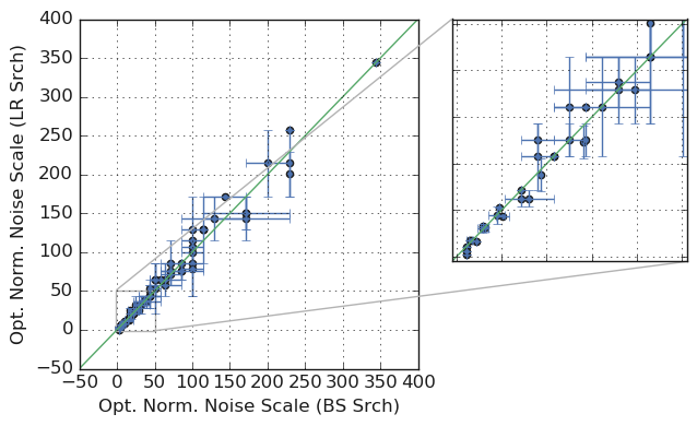
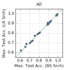
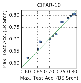
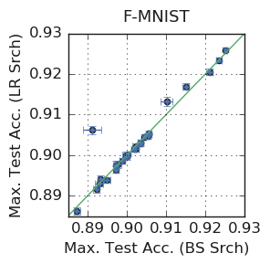
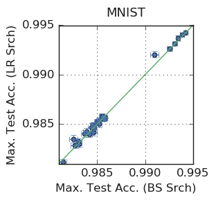
We can verify the validity of our assumption that the set of hyper-parameters yielding optimal performance is given by a level set of , by comparing both the optimal normalized noise scale and the maximum test set accuracy obtained by batch size search and learning rate search. The obtained values for both search methods for all experiments have been plotted against each other in figures 2 and 3. Further evidence for our assumption can be found in section G of the supplementary material. Finally, for each triplet of dataset-network-experiment type, we have plotted the test set accuracy against the scanned parameter (either batch size or learning rate) in figure 8 of section D.
 |
 |
 |
 |
 |
 |
 |
 |
 |
 |
 |
 |
 |
 |
 |
 |
 |
 |
 |
 |
 |
 |
 |
4.2 Standard without Batch Normalization
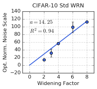
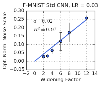
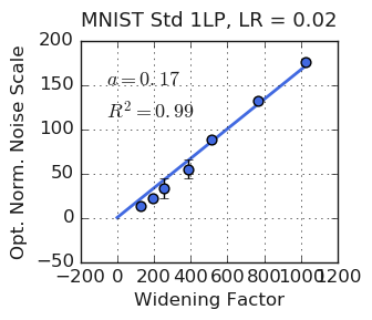
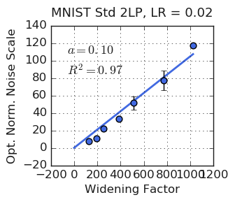
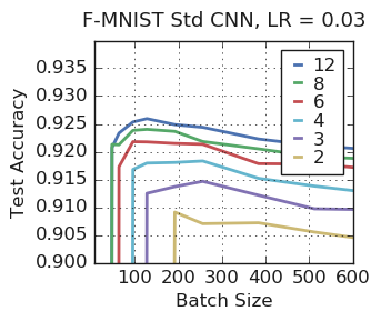
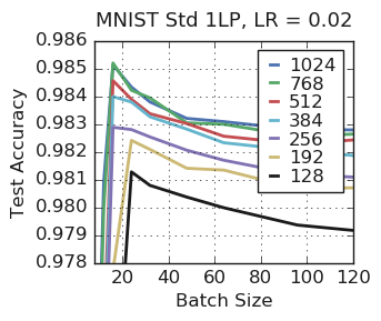
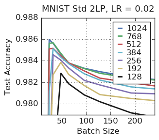
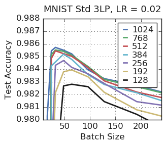
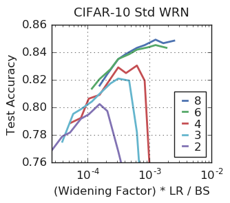
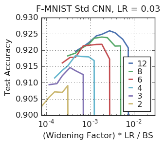
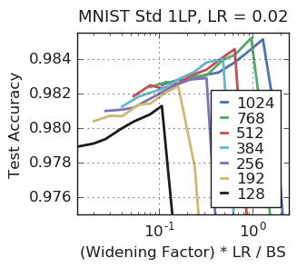
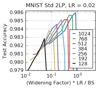
Due to resource constraints, we have only conducted experiments for select dataset-network pairs when using the standard parameterization scheme, shown in figure 4. The optimal normalized noise scale is found using batch size search only. For CIFAR-10 on WRN, networks with were trained with the learning rate , while networks with were trained with a smaller learning rate of due to numerical instabilities (causing high failure rates for wide models when ). Once again, we observe a clear linear relationship between the optimal normalized noise scale and the widening factor. We provide additional experiments incorporating data augmentation, dropout and label smoothing in section F of the supplementary material, which also show the same linear relationship.
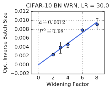
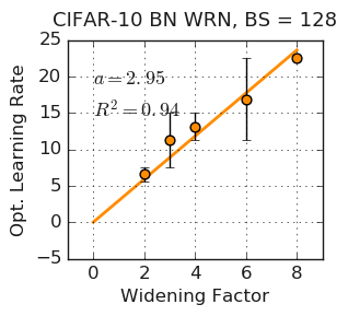
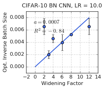
4.3 NTK with Batch Normalization
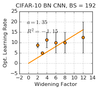
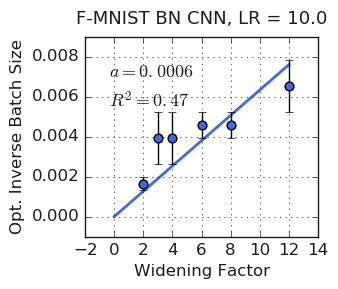
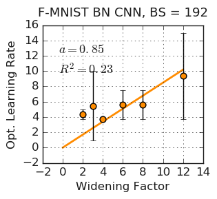
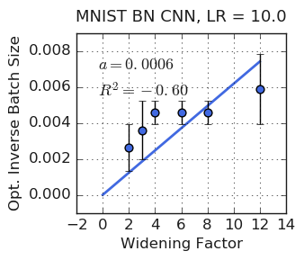
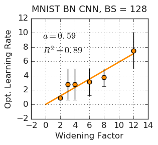
We have only conducted experiments with batch normalization for families of wide residual networks and CNNs. We perform both batch size search and learning rate search. The results of these experiments are summarized in figure 5. Unlike the previous sets of experiments, we do not report an optimal normalized noise scale, as this term is poorly defined when batch normalization is used. Rather, we report the optimal inverse batch size (learning rate) for the given fixed learning rate (batch size) respectively. However as discussed previously, when the batch size is fixed, the SGD noise is still proportional to the learning rate. A clear linear trend is still present for wide residual networks, however this trend is much weaker in the case of convolutional networks.
4.4 Generalization and Network Width
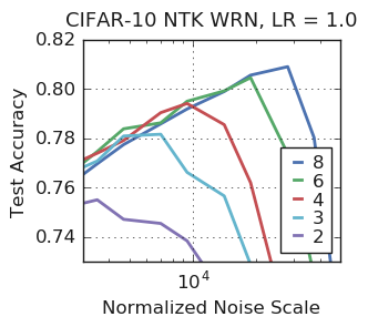
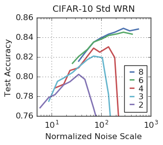
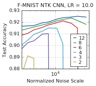
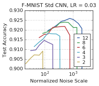
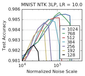
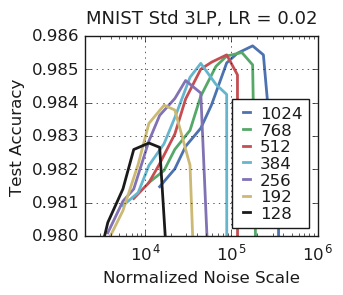
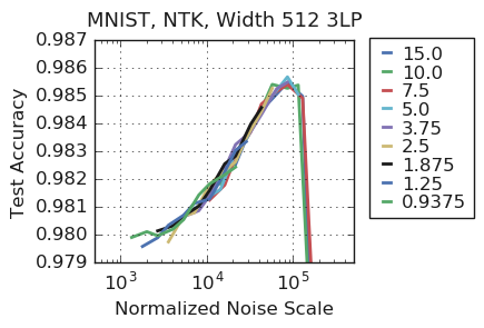
We showed in section 4.1 that in the absence of batch normalization, the test accuracy of a network of a given width is determined by its normalized noise scale. Therefore in figure 6, we plot the test accuracy as a function of noise scale for a range of widths. We include a variety of networks trained without batch normalization with both standard and NTK parameterizations. In all cases the best observed test accuracy increases with width. This is consistent with previous work showing that test accuracy improves with increasing over-parameterization (Neyshabur et al., 2018; Lee et al., 2018; Novak et al., 2018). See section D of the supplementary material for plots of test accuracy in terms of the raw learning rate and batch size instead of noise scale.
More surprisingly, the dominant factor in the improvement of test accuracy with width is usually the increased optimal normalized noise scale of wider networks. To see this, we note that for a given width the test accuracy often improves slowly below the optimum noise scale and then falls rapidly above it. Wider networks have larger optimal noise scales, and this enables their test accuracies to rise higher before they drop. Crucially, when trained at a fixed noise scale below the optimum, the test accuracy is very similar across networks of different widths, and wider networks do not consistently outperform narrower ones. This suggests the empirical performance of wide over-parameterized networks is closely associated with the implicit regularization of SGD.
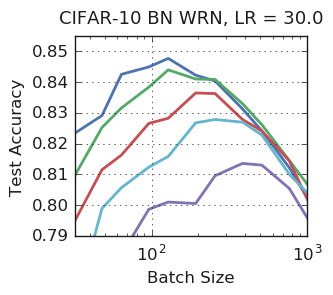
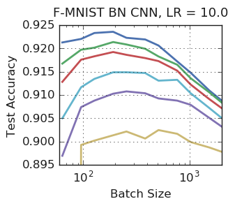
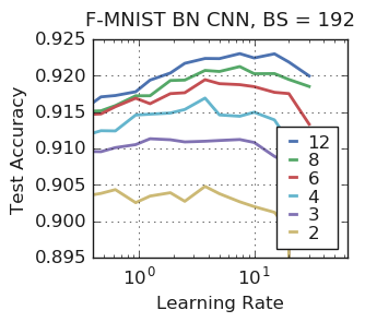
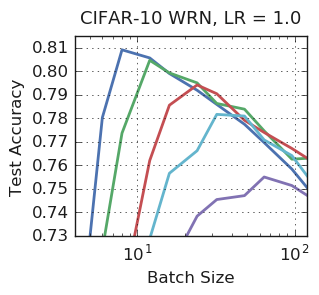
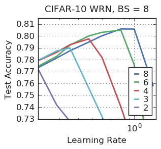
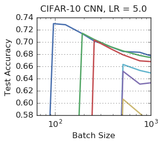
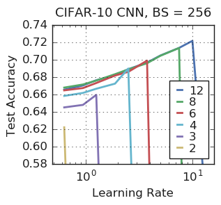
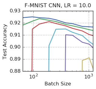
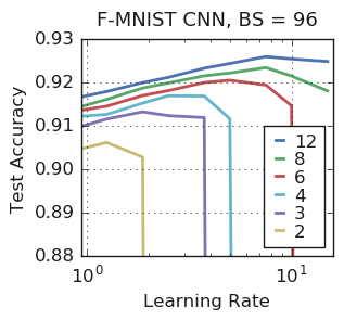
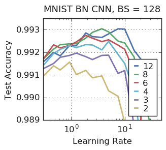
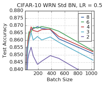
In figure 7 we examine the relationship between generalization and network width for experiments with batch normalization. Since the normalized noise scale is not well-defined, we plot the test accuracy for a range of widths as a function of both the batch size at fixed learning rate, and the learning rate at fixed batch size. We provide plots for WRNs on CIFAR-10 and CNNs on F-MNIST, both in the NTK parameterization. Once again, we find that the best observed test accuracy consistently increases with width. However the qualitative structure of the data differs substantially for the two architectures. In the case of WRNs, we observe similar trends both with and without batch normalization. In the NTK parameterization, wider networks have larger optimal learning rates (smaller optimal batch sizes), and this is the dominant factor behind their improved performance on the test set. For comparison, see figure 8 in section D of the supplementary material for equivalent plots without batch normalization. However in the case of CNNs the behaviour is markedly different, wider networks perform better across a wide range of learning rates and batch sizes. This is consistent with our earlier observation that WRNs obey equation 6 with batch normalization, while CNNs do not.
 |
 |
 |
 |
5 Discussion
Speculations on main result: The proportionality relation (equation 6) between the optimal normalized noise scale and network width holds remarkably robustly in all of our experiments without batch normalization. This relationship provides a simple prescription which predicts how to tune SGD hyper-parameters as width increases. We do not have a theoretical explanation for this phenomenon. However intuitively it appears that noise enhances the final test performance, while the amount of noise a network can tolerate is proportional to the network width. Wider networks tolerate more noise, and thus achieve higher test accuracies. Why SGD noise enhances final performance remains a mystery (Keskar et al., 2016; Sagun et al., 2017; Mandt et al., 2017; Chaudhari & Soatto, 2017; Smith & Le, 2017).
Implications for very wide networks: As noted in the introduction, the largest batch size consistent with equation 6 decreases with width (when training with SGD + momentum without regularization or batch normalization). To clarify this point, we consider NTK networks and standard networks separately. For NTK networks, the learning rate can stay constant with respect to the width without introducing numerical instabilities. As the network gets wider equation 6 requires , which forces the batch size of wide networks to have a small value to achieve optimality. For standard networks, . However in this case the learning rate must decay as the width increases in order for the SGD to remain stable (Karakida et al., 2017). We provide empirical evidence for these stability bounds in section H of the supplementary material. In both cases the batch size must eventually be reduced if we wish to maintain optimal performance as width increases.
Unfortunately we have not yet been able to perform additional experiments at larger widths. However if the trends above hold for arbitrary widths, then there would be a surprising implication. Since the batch size is bounded from below by one, and the normalized learning rate is bounded above by some value due to numerical stability, there is a maximum noise scale we can achieve experimentally. Meanwhile the optimal noise scale increases proportional to the network width. This suggests there may be a critical width for each network family, at which the optimal noise scale exceeds the maximum noise scale, and beyond which the test accuracy does not improve as the width increases, unless additional regularization methods are introduced.
Comments on batch normalization: The analysis of small learning rate SGD proposed by Smith & Le (2017) does not hold with batch normalization, and we therefore anticipated that networks trained using batch normalization might show a different trend. Surprisingly, we found in practice that residual networks trained using batch normalization do follow the trend implied by equation 6, while convolutional networks trained with batch normalization do not.
Conclusion: We introduce the normalized noise scale, which extends the analysis of small learning rate SGD proposed by Smith & Le (2017) to account for the choice of parameterization scheme. We provide convincing empirical evidence that, in the absence of batch normalization, the normalized noise scale which maximizes the test set accuracy is proportional to the network width. We also find that wider networks perform better on the test set. A similar trend holds with batch normalization for residual networks, but not for convolutional networks. We consider two parameterization schemes and three model families including MLPs, ConvNets and ResNets. Since the largest stable learning rate is bounded, the largest batch size consistent with the optimal noise scale decreases as the width increases.
Acknowledgements
We thank Yasaman Bahri, Soham De, Boris Hanin, Simon Kornblith, Jaehoon Lee, Luke Metz, Roman Novak, George Philipp, Ben Poole, Chris Shallue, Ola Spyra, Olga Wichrowska and Sho Yaida for helpful discussions.
References
- Bartlett et al. (2017) Bartlett, P. L., Foster, D. J., and Telgarsky, M. J. Spectrally-normalized margin bounds for neural networks. In Advances in Neural Information Processing Systems, pp. 6240–6249, 2017.
- Chaudhari & Soatto (2017) Chaudhari, P. and Soatto, S. Stochastic gradient descent performs variational inference, converges to limit cycles for deep networks. CoRR, abs/1710.11029, 2017. URL http://arxiv.org/abs/1710.11029.
- Dziugaite & Roy (2017) Dziugaite, G. K. and Roy, D. M. Computing nonvacuous generalization bounds for deep (stochastic) neural networks with many more parameters than training data. arXiv preprint arXiv:1703.11008, 2017.
- Glorot & Bengio (2010) Glorot, X. and Bengio, Y. Understanding the difficulty of training deep feedforward neural networks. In AISTATS 2010, 2010.
- Goyal et al. (2017) Goyal, P., Dollár, P., Girshick, R. B., Noordhuis, P., Wesolowski, L., Kyrola, A., Tulloch, A., Jia, Y., and He, K. Accurate, large minibatch SGD: training imagenet in 1 hour. CoRR, abs/1706.02677, 2017. URL http://arxiv.org/abs/1706.02677.
- Harvey et al. (2017) Harvey, N., Liaw, C., and Mehrabian, A. Nearly-tight vc-dimension bounds for piecewise linear neural networks. In Conference on Learning Theory, pp. 1064–1068, 2017.
- He et al. (2015) He, K., Zhang, X., Ren, S., and Sun, J. Delving deep into rectifiers: Surpassing human-level performance on imagenet classification. CoRR, abs/1502.01852, 2015. URL http://arxiv.org/abs/1502.01852.
- He et al. (2016) He, K., Zhang, X., Ren, S., and Sun, J. Deep residual learning for image recognition. In Proceedings of the IEEE conference on computer vision and pattern recognition, pp. 770–778, 2016.
- Ioffe & Szegedy (2015) Ioffe, S. and Szegedy, C. Batch normalization: Accelerating deep network training by reducing internal covariate shift. CoRR, abs/1502.03167, 2015. URL http://arxiv.org/abs/1502.03167.
- Jacot et al. (2018) Jacot, A., Gabriel, F., and Hongler, C. Neural tangent kernel: Convergence and generalization in neural networks. CoRR, abs/1806.07572, 2018. URL http://arxiv.org/abs/1806.07572.
- Jastrzebski et al. (2017) Jastrzebski, S., Kenton, Z., Arpit, D., Ballas, N., Fischer, A., Bengio, Y., and Storkey, A. J. Three factors influencing minima in SGD. CoRR, abs/1711.04623, 2017. URL http://arxiv.org/abs/1711.04623.
- Karakida et al. (2017) Karakida, R., Akaho, S., and ichi Amari, S. Universal statistics of fisher information in deep neural networks: Mean field approach. arXiv preprint arXiv:, abs/1806.01316, 2017. URL http://arxiv.org/abs/1806.01316.
- Karras et al. (2017) Karras, T., Aila, T., Laine, S., and Lehtinen, J. Progressive growing of gans for improved quality, stability, and variation. CoRR, abs/1710.10196, 2017. URL http://arxiv.org/abs/1710.10196.
- Karras et al. (2018) Karras, T., Laine, S., and Aila, T. A style-based generator architecture for generative adversarial networks. CoRR, abs/1812.04948, 2018. URL http://arxiv.org/abs/1812.04948.
- Keskar et al. (2016) Keskar, N. S., Mudigere, D., Nocedal, J., Smelyanskiy, M., and Tang, P. T. P. On large-batch training for deep learning: Generalization gap and sharp minima. arXiv preprint arXiv:1609.04836, 2016.
- Krizhevsky (2009) Krizhevsky, A. Learning multiple layers of features from tiny images. 2009.
- LeCun et al. (1996) LeCun, Y., Bottou, L., Orr, G. B., and Müller, K.-R. Effiicient backprop. In Neural Networks: Tricks of the Trade, 1996.
- Lecun et al. (1998) Lecun, Y., Bottou, L., Bengio, Y., and Haffner, P. Gradient-based learning applied to document recognition. In Proceedings of the IEEE, pp. 2278–2324, 1998.
- LeCun et al. (2010) LeCun, Y., Cortes, C., and Burges, C. J. MNIST handwritten digit database. 2010. URL http://yann.lecun.com/exdb/mnist/.
- Lee et al. (2018) Lee, J., Bahri, Y., Novak, R., Schoenholz, S., Pennington, J., and Sohl-dickstein, J. Deep neural networks as gaussian processes. In International Conference on Learning Representations, 2018. URL https://openreview.net/forum?id=B1EA-M-0Z.
- Mandt et al. (2017) Mandt, S., Hoffman, M. D., and Blei, D. M. Stochastic gradient descent as approximate bayesian inference. arXiv preprint arXiv:, abs/1704.04289, 2017. URL http://arxiv.org/abs/1704.04289.
- McCandlish et al. (2018) McCandlish, S., Kaplan, J., Amodei, D., and Team, O. D. An empirical model of large-batch training. CoRR, abs/1812.06162, 2018. URL http://arxiv.org/abs/1812.06162.
- Nagarajan & Kolter (2018) Nagarajan, V. and Kolter, Z. Deterministic pac-bayesian generalization bounds for deep networks via generalizing noise-resilience. 2018.
- Neyshabur et al. (2017) Neyshabur, B., Bhojanapalli, S., and Srebro, N. A pac-bayesian approach to spectrally-normalized margin bounds for neural networks. arXiv preprint arXiv:1707.09564, 2017.
- Neyshabur et al. (2018) Neyshabur, B., Li, Z., Bhojanapalli, S., LeCun, Y., and Srebro, N. Towards understanding the role of over-parametrization in generalization of neural networks. arXiv preprint arXiv:1805.12076, 2018.
- Novak et al. (2018) Novak, R., Bahri, Y., Abolafia, D. A., Pennington, J., and Sohl-Dickstein, J. Sensitivity and generalization in neural networks: an empirical study. In International Conference on Learning Representations, 2018. URL https://openreview.net/forum?id=HJC2SzZCW.
- Sagun et al. (2017) Sagun, L., Evci, U., Guney, V. U., Dauphin, Y., and Bottou, L. Empirical analysis of the hessian of over-parametrized neural networks. arXiv preprint arXiv:1706.04454, 2017.
- Schoenholz et al. (2016) Schoenholz, S. S., Gilmer, J., Ganguli, S., and Sohl-Dickstein, J. Deep information propagation. CoRR, abs/1611.01232, 2016. URL http://arxiv.org/abs/1611.01232.
- Sculley et al. (2018) Sculley, D., Snoek, J., Wiltschko, A. B., and Rahimi, A. Winner’s curse? on pace, progress, and empirical rigor. In ICLR (Workshop) Sculley et al. (2018). URL http://dblp.uni-trier.de/db/conf/iclr/iclr2018w.html#SculleySWR18.
- Shallue et al. (2018) Shallue, C. J., Lee, J., Antognini, J. M., Sohl-Dickstein, J., Frostig, R., and Dahl, G. E. Measuring the effects of data parallelism on neural network training. CoRR, abs/1811.03600, 2018. URL http://arxiv.org/abs/1811.03600.
- Smith & Le (2017) Smith, S. L. and Le, Q. V. A bayesian perspective on generalization and stochastic gradient descent. CoRR, abs/1710.06451, 2017. URL http://arxiv.org/abs/1710.06451.
- Smith et al. (2017) Smith, S. L., Kindermans, P., and Le, Q. V. Don’t decay the learning rate, increase the batch size. CoRR, abs/1711.00489, 2017. URL http://arxiv.org/abs/1711.00489.
- Soudry et al. (2018) Soudry, D., Hoffer, E., Nacson, M. S., Gunasekar, S., and Srebro, N. The implicit bias of gradient descent on separable data. The Journal of Machine Learning Research, 19(1):2822–2878, 2018.
- van Laarhoven (2017) van Laarhoven, T. L2 regularization versus batch and weight normalization. CoRR, abs/1706.05350, 2017. URL http://arxiv.org/abs/1706.05350.
- Wilson et al. (2017) Wilson, A. C., Roelofs, R., Stern, M., Srebro, N., and Recht, B. The marginal value of adaptive gradient methods in machine learning. In Advances in Neural Information Processing Systems, pp. 4148–4158, 2017.
- Xiao et al. (2017) Xiao, H., Rasul, K., and Vollgraf, R. Fashion-mnist: a novel image dataset for benchmarking machine learning algorithms. CoRR, abs/1708.07747, 2017. URL http://arxiv.org/abs/1708.07747.
- Yaida (2018) Yaida, S. Fluctuation-dissipation relations for stochastic gradient descent. arXiv preprint arXiv:, abs/1810.00004, 2018. URL http://arxiv.org/abs/1810.00004.
- Zagoruyko & Komodakis (2016) Zagoruyko, S. and Komodakis, N. Wide residual networks. CoRR, abs/1605.07146, 2016. URL http://arxiv.org/abs/1605.07146.
- Zhang et al. (2016) Zhang, C., Bengio, S., Hardt, M., Recht, B., and Vinyals, O. Understanding deep learning requires rethinking generalization. CoRR, abs/1611.03530, 2016. URL http://arxiv.org/abs/1611.03530.
- Zhou et al. (2018) Zhou, W., Veitch, V., Austern, M., Adams, R. P., and Orbanz, P. Non-vacuous generalization bounds at the imagenet scale: a pac-bayesian compression approach. 2018.
Appendix A Networks and Datasets
We consider MLPs with 1, 2 or 3 hidden layers. Each layer has the same number of hidden units, . We denote the -layered perceptron with width by the label . We do not consider batch normalization for these networks, and we consider the range of widths,
| (13) |
We consider a family of convolutional networks , obtained from LeNet-5 (figure 2 of Lecun et al. (1998)) by scaling all the channels, as well as the widths of the fully connected layers, by a widening factor of (the factor of allows integer for all experiments). Thus, LeNet-5 is identified as CNN2. We also consider batch normalization, which takes place after the dense or convolutional affine transformation, and before the activation function, as is standard. We do not use biases when we use batch normalization. We consider the widening factors,
| (14) |
Finally, we consider a family of wide residual networks , where is equivalent to table 1 of Zagoruyko & Komodakis (2016) if and . For consistency with Zagoruyko & Komodakis (2016) the first wide ResNet layer, a 3 to 16 channel expansion, is not scaled with . As for CNNs, we study WRNs both with and without batch normalization. We consider the widening factors,
| (15) |
The training sets of MNIST and Fashion-MNIST have been split into training-validation sets of size 55000-5000 while for CIFAR-10, the split is given by 45000-5000. We have used the official test set of 10000 images for each dataset. For MNIST and F-MNIST, we normalize the pixels of each image to range from -0.5 to 0.5. For CIFAR-10, we normalize the pixels to have zero mean and unit variance. We do not use data augmentation for any of the experiments presented in the main text.
Appendix B Training Time for Experiments
For experiments with fixed learning rate , we set the number of training steps by setting both an epoch bound and a step bound . So for a given batch size the number of training steps is set by,
| (16) |
After running the batch size search, we may choose a reasonable batch size to hold fixed during learning search rate. Experiments with fixed batch size and variable learning rate are always paired to such a “parent experiment.” When the batch size is fixed and the learning rate varies, we must scale the number of training steps proportional to the learning rate. We pick the reference learning rate to be the learning rate at which the original batch size search was run, and a reference number of training steps , which is computed at the fixed batch size using the epoch and step bound provided in equation 16. Then for learning rate , the number of training steps is given by
| (17) |
That is, for learning rates larger than we perform updates, while for learning rates smaller than , we scale the number of updates inversely proportional to the learning rate.
Appendix C Experiment Details and Configurations
In this section we detail the specific configurations of experiments run in this work.
C.1 NTK without Batch Normalization
| Dataset | Networks | ||||||
|---|---|---|---|---|---|---|---|
| MNIST | 1LP | 120 | 80k | 10.0 | 8 | 10.0 | 825k |
| MNIST | 2LP | 120 | 80k | 10.0 | 16 | 10.0 | 412.5k |
| MNIST | 3LP | 120 | 80k | 10.0 | 16 | 10.0 | 412.5k |
| MNIST | CNN | 120 | 80k | 10.0 | 24 | 10.0 | 275k |
| F-MNIST | 1LP | 240 | 160k | 10.0 | 12 | 10.0 | 1100k |
| F-MNIST | 2LP | 240 | 160k | 10.0 | 24 | 10.0 | 550k |
| F-MNIST | 3LP | 240 | 160k | 10.0 | 48 | 10.0 | 275k |
| F-MNIST | CNN | 240 | 160k | 10.0 | 96 | 10.0 | 160k |
| CIFAR-10 | CNN | 540 | 320k | 5.0 | 256 | 10.0 | 160k |
| CIFAR-10 | WRN | 270 | 80k | 1.0 | 8 | 1.0 | 1500k |
We run both batch size search and learning rate search to determine the optimal normalized noise scale for networks trained with NTK parameterization and without batch normalization. The relevant parameters used for the search experiments are listed in table 1. The scalar denotes the fixed learning rate used for batch size search, while denotes the fixed batch size used during learning rate search.
The epoch bound and the training step bound are defined in section B of the supplementary material. Also as we explained in section B, the training time is scaled with respect to a reference training time and a reference learning rate for the learning rate search experiments. These are denoted and in the table respectively.
C.2 Standard without Batch Normalization
| Dataset | Networks | ||||
|---|---|---|---|---|---|
| MNIST | MLP | All | 120 | 80k | 0.02 |
| F-MNIST | CNN | All | 480 | 320k | 0.03 |
| CIFAR-10 | WRN | 2, 3, 4 | 540 | 160k | 0.0025 |
| CIFAR-10 | WRN | 6, 8 | 1080 | 320k | 0.00125 |
For standard networks without batch normalization, we only carry out batch size search experiments at a fixed learning rate . For CIFAR-10 experiments on wide residual networks, we chose to use two different learning rates depending on the width of the networks (narrower networks can be trained faster with a bigger learning rate, while wider networks require a smaller learning rate for numerical stability). The experiment configurations are listed in table 2.
C.3 NTK with Batch Normalization
| Dataset | Networks | ||||||
|---|---|---|---|---|---|---|---|
| MNIST | CNN | 120 | 80k | 10.0 | 128 | 10.0 | 80k |
| F-MNIST | CNN | 480 | 320k | 10.0 | 192 | 10.0 | 320k |
| CIFAR-10 | CNN | 540 | 320k | 10.0 | 192 | 10.0 | 320k |
| CIFAR-10 | WRN | 270 | 80k | 30.0 | 192 | 30.0 | 80k |
The experiment configurations for networks parameterized using the NTK scheme with batch normalization are listed in table 3. Both batch size search and learning rate search have been carried out. The parameters defined are equivalent to those used for NTK networks without batch normalization in section C.1.
Appendix D Plots from Batch Search and Learning Rate Search
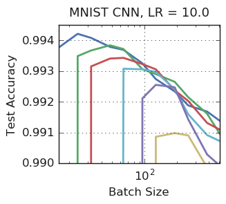
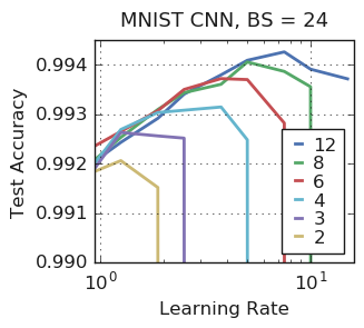
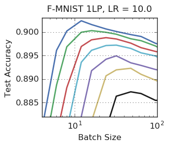
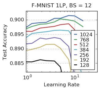
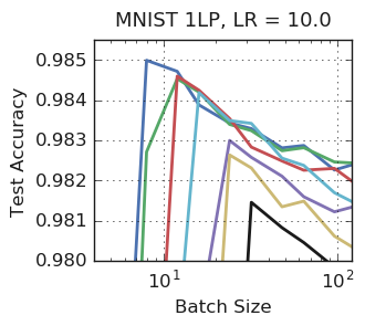
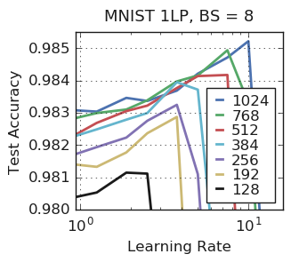
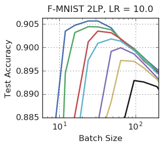
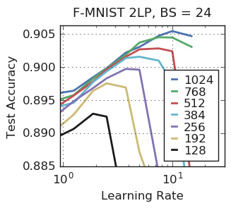
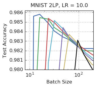
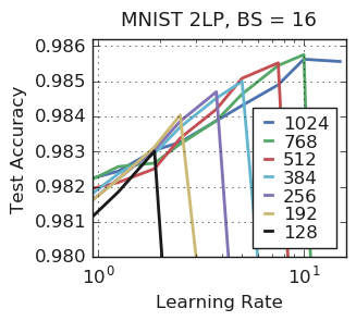
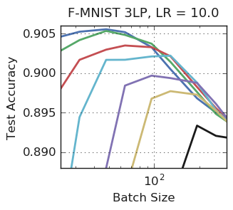
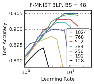
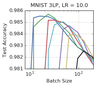
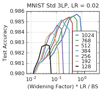
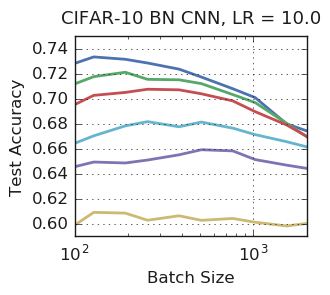
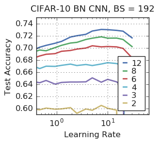
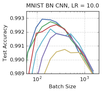
In this section, we present plots of the average test set accuracy vs. batch size/learning rate for batch size/learning rate search experiments with fixed learning rate/batch size respectively. All the learning rate search experiments are paired with batch size search experiments, and share the same color-code and legend describing the network widening factors.
 |
 |
 |
 |
 |
 |
 |
 |
 |
 |
 |
 |
 |
 |
 |
 |
 |
 |
 |
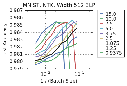
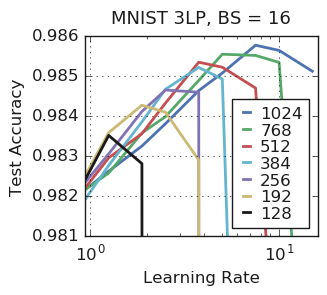 |
Figure 8 plots the results of batch size/learning rate search experiments run with NTK-parameterized networks without batch normalization. Here, the x-axis is plotted in log-scale. Since , if the performance of the network is determined by the noise scale, then the figures for batch size search and learning rate search experiments on the same dataset-network pair should be symmetric to one another. This symmetry is nicely on display in figure 8.
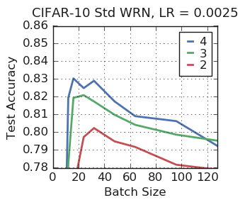
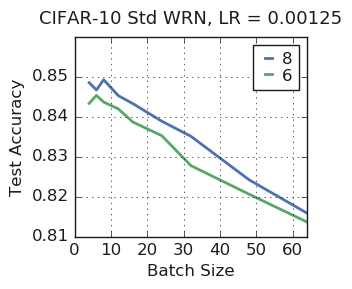
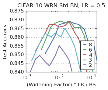
Figure 9 plots batch size search experiments run with standard parameterization and without batch normalization. Standard-parameterized WRN6 and WRN8 were run with a reduced learning rate due to numerical stability issues, and the results of their batch size search experiments have been plotted separately. In contrast to NTK-parameterized networks, the normalized noise is width-dependent for networks parameterized using the standard scheme. Also, we have batch searches conducted over varying learning rates in one instance. Thus it is more informative to put everything together and plot the performance of the network against . This has been done in figure 10. This plot reproduces the qualitative features of figure 8, which is strong evidence for being the correct indicator of the performance of networks within a linear family.
Figure 11 plots the results of batch size/learning rate search run with NTK-parameterized networks with batch normalization.
When both batch size and learning rate search have been carried out, the y-axes of the plots, along which the network performance is plotted, are aligned so that the maximal performance obtained from the search can be compared.
 |
 |
 |
 |
 |
 |
 |
 |
 |
 |
 |
|
|
 |
 |
|
|
 |
 |
Appendix E Networks with Standard Parameterization and Batch Normalization
In this section, we present results of batch search experiments with WRNs with batch normalization that are parameterized using the standard scheme. We train with a constant schedule with epoch bound and step bound k.
 |
 |
 |
As was with the case with NTK parameterized WRNs, the scaling rule for the optimum batch size coincides with that of the case when batch normalization is absent, i.e., the optimal batch size is constant with respect to the widening factor.
Appendix F Batch Search Experiments with Regularization
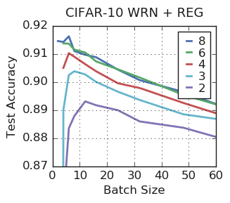
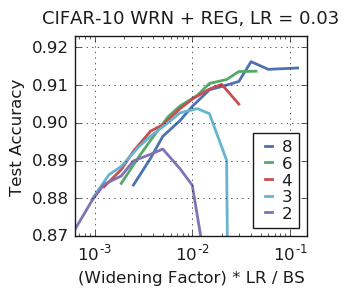
In this section, we present the results of training WRNs on CIFAR-10 with regularization. We use dropout with probability and label smoothing with uncertainty . Data augmentation is also applied by first taking a random crop of the image padded by 4 pixels and then applying a random flip. Note that we have chosen these regularization schemes because we do not anticipate that the associated hyper-parameters will depend strongly on the network width or the noise scale.
We carry out batch search experiments for WRNs parameterized in the standard scheme on CIFAR-10, with epoch bound and step bound k. The results are given in figure 13. We have used the fixed learning rate .
 |
 |
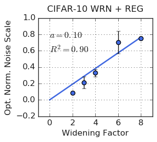 |
The scaling rule still holds in the presence of these three regularizers. The use of regularization schemes significantly increases the final test accuracies, however these test accuracies still depend strongly on the SGD noise scale.
Appendix G The Performance of 3LP on a 2D Grid of Learning Rates and Batch Sizes
Our main result (equation 6) is based on the theory of small learning rate SGD, which claims that the final performance of models trained using SGD is controlled solely by the noise scale . To provide further evidence for this claim, here we consider 3LP512 and measure its performance on MNIST across a 2D grid of batch sizes and a range of learning rates as indicated in figure 14. We run 20 experiments for each learning rate/batch size pair and compute the mean test set accuracy. We set the epoch bound to and the training set bound with and . The results are shown in figure 14, where we plot the performance curves as a function of the batch size and the noise scale. As expected, the final test accuracy is governed solely by the noise scale.
 |
 |
Appendix H Numerical Stability and the Normalized Learning Rate
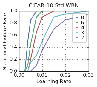
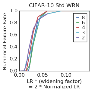
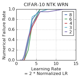
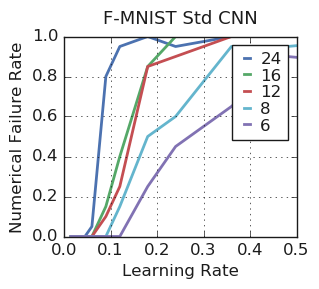
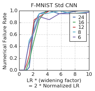
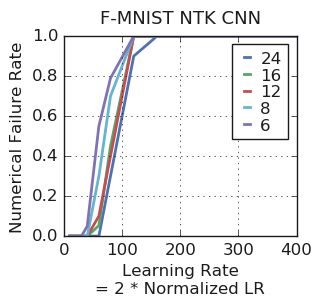
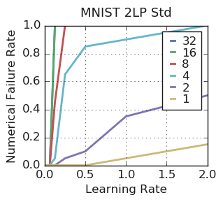
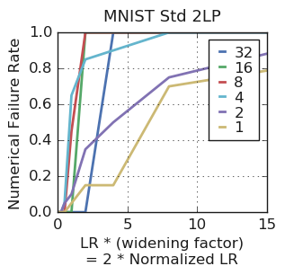
In this section, we present experiments to verify the claim that (in the absence of batch normalization), numerical instabilities affect training when , where is constant with respect to the width for NTK parameterization while as for networks parameterized using the standard scheme. This is equivalent to saying that the scale at which the normalized learning rate becomes unstable is constant with respect to the width of the network.
To do so, we take families of NTK and standard parameterized networks, and compute the failure rate after 20 epochs of training with a fixed batch size (64) at a range of learning rates. For each network, we run 20 experiments, and compute the failure rate, which is defined to be the portion of experiments terminated by a numerical error. We run the experiments for CIFAR-10 on WRNw (), F-MNIST on CNNw () and MNIST on 2LP512⋅w ().
For CNNs and 2-layer perceptrons, we consider much wider networks than are studied in the main text. This is because we are ultimately interested in observing numerical instabilities which occur when is large. For the purpose of studying this break-down of numerical stability, we can afford to use much wider networks. The width dependence of becomes more evident by focusing on these wide networks, as the behaviour of narrow networks is less predictable.
Figure 15 depicts 3 figures for each dataset-network combination. The first figure shows the failure rate plotted against the learning rate for networks using the standard parameterization. The second is the failure rate plotted against the product of the learning rate and the widening factor—i.e., twice the normalized learning rate—for the same networks (trained using the standard parameterization). The third figure shows the failure rate plotted against the learning rate for networks parameterized using the NTK scheme. Here, the normalized learning rate is simply half the learning rate.
 |
 |
 |
 |
 |
 |
 |
 |
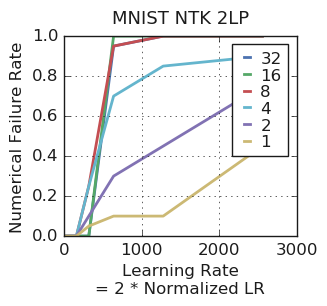 |
It is clear from these plots that is independent of the widening factor for WRNs and CNNs, while the definition of for the 2LP seems more subtle. Nevertheless for all three network families, we see similar stability curves as width increases for both parameterization schemes, when measured as a function of the normalized learning rate.
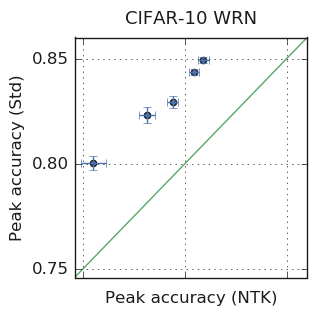
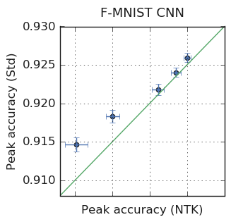
Appendix I Performance Comparison between NTK Networks and Standard Networks
Here we provide a brief comparison of the performance of both parameterization schemes on the test set. In figure 16, the peak test accuracy of a network parameterized with the standard scheme is plotted against the peak test accuracy obtained when the same network is parameterized with the NTK scheme. The dataset-network pairs are indicated in the title—CIFAR-10 on WRNw, F-MNIST on CNNw and MNIST on MLPs. We see that standard parameterization consistently out-performs NTK parameterization on WRNs and CNNs, although the performance is comparable for MNIST on MLPs.
 |
 |
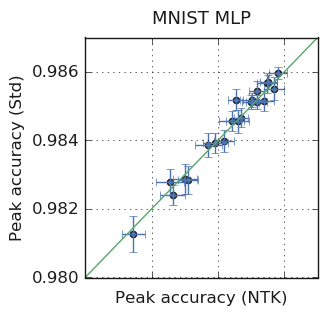 |
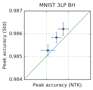
The reason that performance agrees well for the particular MLPs investigated in the main text of the paper, is because all the hidden layers have equal width. In this limit, NTK parameterization and standard parameterization are essentially identical. However by varying the network architecture, we can observe a discrepancy between the performance of MLPs as well. As an example, we consider the following bottom-heavy (BH) and top-heavy (TH) 3LPs with hidden layer widths,
| (18) |
We consider the widening factors . In figure 17, we display the discrepancy between the performance between both bottom-heavy and top-heavy networks parameterized in the NTK and standard schemes.
 |
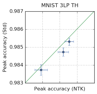 |
In the bottom heavy case, MLPs parameterized in the standard scheme appear to outperform MLPs parameterized in the NTK scheme. However in the top heavy case, MLPs parameterized in the NTK scheme appear to outperform MLPs parameterized in the standard scheme. These results suggest that neither scheme is superior to the other, but that the final performance will depend on the combination of parameterization scheme, initialization conditions and network architecture. We note that we initialize all our networks at critical initialization (), and that this overall weight scale was not tuned.