Measuring Spin of the Remnant Black Hole from Maximum Amplitude
Abstract
Gravitational waves emitted during the merger of two black holes carry information about the remnant black hole, namely its mass and spin. This information is typically found from the ringdown radiation as the black hole settles to a final state. We find that the remnant black hole spin is already known at the peak amplitude of the gravitational wave strain. Using this knowledge, we present a new method for measuring the final spin that is template independent, using only the chirp mass, the instantaneous frequency of the strain and its derivative at maximum amplitude, all template independent.
pacs:
04.80.Nn, 04.25.dg, 04.25.D-, 04.30.-wI Introduction
The advent of gravitational wave (GW) astronomy has granted us the opportunity to observationally study compact binary coalescences. During the course of the first two observing runs, LIGO Aasi et al. (2015) and Virgo Acernese et al. (2015) detected GWs from a total of ten coalescing binary black holes (BBHs) and one binary neutron star The LIGO Scientific Collaboration and the Virgo Collaboration (2018); Collaboration and Collaboration (2017). These systems have hinted at the population properties of BBHs such as the distributions of mass, spin and redshifts The LIGO Scientific Collaboration and The Virgo Collaboration (2018), and have placed GW observations into the new era of multi-messenger astronomy Collaboration and Collaboration (2017); Maészàros et al. (2019).
In the few years since the first detection of GWs Collaboration and Collaboration (2016), we have learned a tremendous amount about the parameter space of stellar-mass black holes (BHs) The LIGO Scientific Collaboration and The Virgo Collaboration (2018). Each stage of the coalescence provides information about the BBH system; this study focuses on the parameters describing the remnant BH. The product of a BBH merger is a perturbed BH that emits ringdown radiation as it settles to a Kerr BH. This process provides fundamental information to understand gravity in its most extreme regime. Perturbation theory tells a compelling story about how perturbed BHs, like the remnant of a BBH merger, lose the information about the disturbance, often called hair, in the form of GWs Vishveshwara (1970). Perturbed BHs ring down or emit GWs with a frequency () and decay time () characterized by the BH mass and spin Press (1971), providing the means to determine the remnant BH parameters upon the detection of GWs.
The GW during this ringdown phase is generally represented as the sum of quasi-normal modes (QNMs), each expressible as a damped sinusoid with its own and , fixed by the mass and spin of the final BH Nollert and Price (1999); Kokkotas and Schmidt (1999); Berti et al. (2009). The Echeverria formulas Echeverria (1989) provide relationships to determine the BH mass and spin from and using spheroidal harmonics.
There have been attempts to measure and of the ringdown Abbott et al. (2009); Goggin and the LIGO Scientific Collaboration (2006); Berti et al. (2007); Carullo et al. (2019a); Yang et al. (2017); Nakano et al. (2018); Cabero et al. (2018) and as the detectors improve in sensitivity, this will become more viable. One commonly considered method is to estimate the ringdown parameters by matching directly to the exponentially decaying ringdown, where Ref.Carullo et al. (2019a) finds consistent results for GW150914 searching for damped sinusoids. The possibility of using GWs to detect this spectrum of radiation is often referred to as BH spectroscopy Dreyer et al. (2004); Berti et al. (2006); Brito et al. (2018). The short duration and low-amplitude of the signal expected from stellar-mass mergers, however, makes this post-merger phase challenging to detect, which is further compounded by the reliance upon knowing when ringdown begins Bhagwat et al. (2018); Carullo et al. (2018).
Due to these challenges, current approaches Abbott et al. (2016); Healy et al. (2014); Rezzolla et al. (2008) to estimate the spin of the final BH match the data to theoretical models of the inspiral. Fortunately, numerical relativity (NR) provides the map from initial to final parameters Healy and Lousto (2017); Jiménez-Forteza et al. (2017); Hofmann et al. (2016) that are used to estimate the final spin. For systems with many cycles of inspiral, this method can predict the remnant spin with precision, assuming general relativity (GR). It is desirable to obtain the remnant spin independently of matched filtering of either the inspiral or ringdown in order to perform tests of GR Abbott et al. (2016, 2019); Ghosh et al. (2018, 2016). One can also perform tests of GR directly from the peak frequency Carullo et al. (2019b).
With the goal of avoiding the use of the exponentially decaying ringdown, we propose a method of determining the final spin that takes advantage of the higher amplitude at the merger of two BHs. The method proposed here builds on earlier work by Healy et al Healy et al. (2014) which connected the instantaneous frequency of the GW at peak amplitude to and of the ringdown. While it is not obvious that such a relationship should exist, there have been hints of the merged black hole entering a perturbative regime as early as the peak amplitude Buonanno et al. (2007); Kamaretsos et al. (2012); Healy et al. (2014); Giesler et al. (2019) with the radiation near the peak amplitude of the strain being described by QNMs that include the overtones. In this paper, we find that the spin of the remnant black hole is already known at the peak amplitude.
Inspired by the results of Healy et al, we create a map linking the instantaneous frequency at maximum amplitude (), the derivative of the instantaneous frequency at maximum amplitude (), and the chirp mass () to the dimensionless remnant spin (). One advantage of this method is that all measurements involved, , , and , are independent of fitting the data to a model waveform. Furthermore, has the advantage of needing only a few pre-peak cycles to obtain a good measurement using a well known gravitational-wave algorithm, Coherent WaveBurst (cWB) Tiwari et al. (2016). In the following we: a) demonstrate a tight relation between the frequency properties measured at peak and the spin of the final BH and b) develop an algorithm to exploit this relationship on GW observations.
In the Methodology section, we describe the NR data used to derive a connection from , , to and discuss the associated errors. In the Final Spin section, we examine the viability of the relationship as a form of parameter estimation with noisy data. Finally, we summarize our findings in the Conclusions section.
II Methodology
II.1 NR Catalog and Errors
The relationships found in this paper are based upon the use of 112 NR simulations provided by the Georgia Tech waveform catalog, 47 of which are nonspinning and 65 of which are aligned spin, with mass ratios Jani et al. (2016). The Georgia Tech waveforms are produced using the MAYA code Herrmann et al. (2007); Vaishnav et al. (2007); Healy et al. (2009); Pekowsky et al. (2013a), a branch of the Einstein Toolkit Loffler et al. (2012), a NR code built upon Cactus with mesh refinement from Carpet Schnetter et al. (2004) with the addition of thorns to calculate various quantities during the simulation including an apparent horizon solver Thornburg (2004).
We create a map from , , to . As will be described in subsection “Fitting to final spin,” this equates to a mapping from the dimensionless instantaneous frequency at maximum amplitude (), the derivative of the dimensionless instantaneous frequency at maximum amplitude (), and the symmetric mass ratio () to .
In order to create this mapping, , , and are obtained from the NR simulation data. In this paper we use the strain, , for ease of working with the GW detectors, given
and computed according to Reisswig and Pollney (2011). Strain is represented as a sum of spin-weighted spherical harmonics given by
where are excited depending on the inspiral parameters and the binary’s orientation with respect to the observer. In aligned spin scenarios and face on orientations, the , m=2 mode dominates the signal; and, therefore, this study uses only the , mode Calderón Bustillo et al. (2017, 2016); Pekowsky et al. (2013b); Varma and Ajith (2017).
The GW amplitude is thus , and the instantaneous frequency is found as the derivative of the phase, i.e. where . and are obtained simply by identifying the time at which the amplitude reaches a maximum and grabbing the instantaneous frequency and its time derivative at that time. This is shown visually in Fig. 1.
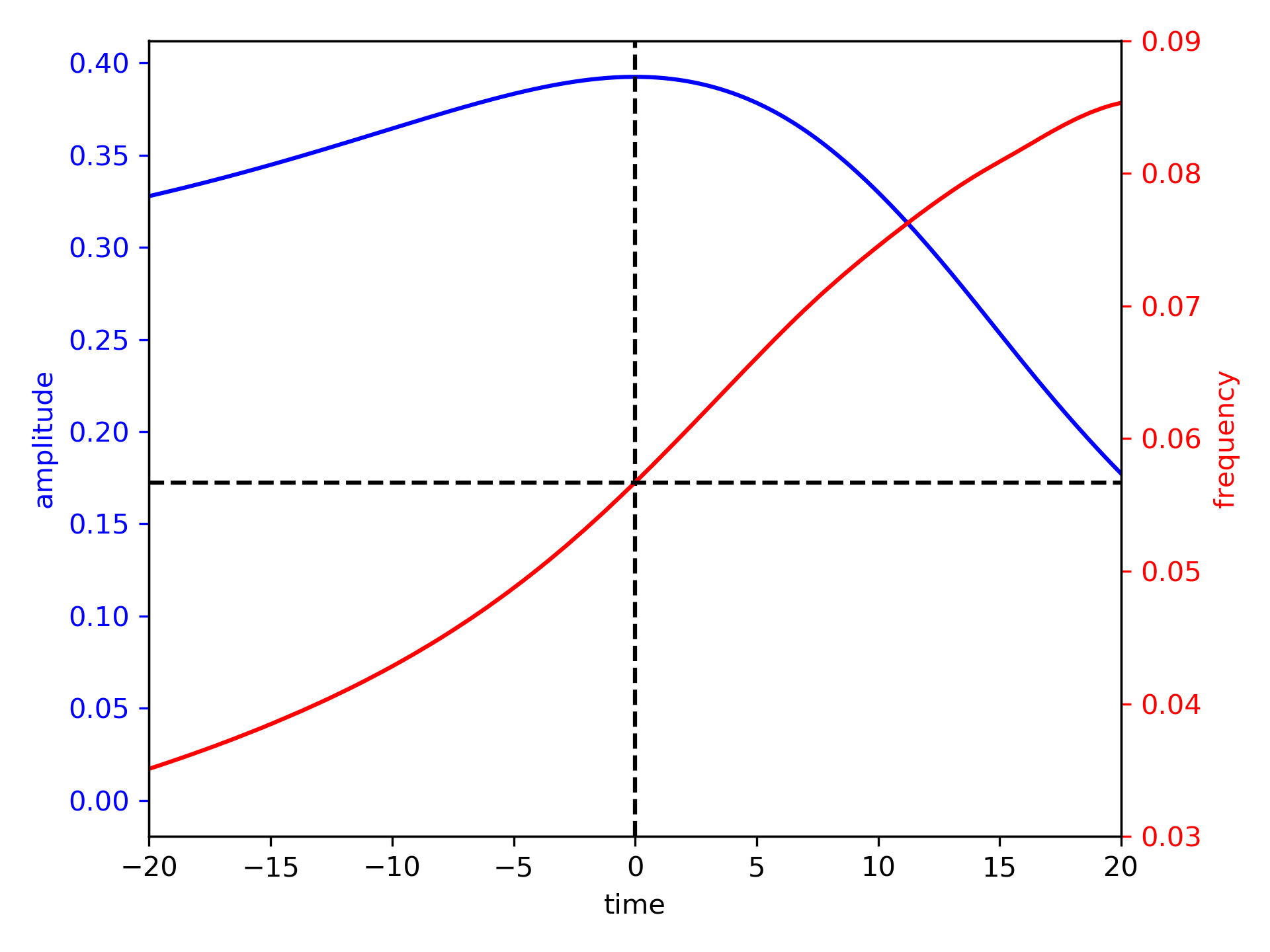
Note is determined from the apparent horizon of the remnant BH.
The finite spatial and temporal resolutions of NR simulations introduce systematic uncertainty into the estimates of frequency and spin. By repeating each simulation at multiple resolutions, the error is found to be of order 0.01% for , 1% for , and 1.4% for . These uncertainties account for the spread in the fit shown in Fig. 2.
II.2 Fitting to final spin
With the data selected and the NR errors understood, we can create a fit that connects the peak amplitude of GW strain to the final BH spin. In order to create this fitting from , , and to using NR simulations, we utilize the following relationships
| (1) |
| (2) |
where is the symmetric mass ratio defined as a function of the initial masses, and :
| (3) |
and is the chirp mass expressible as:
| (4) |
These lead us to plot the spin of the remnant BH against a function of and which will take the form
| (5) |
The resulting fit is shown in Fig 2.
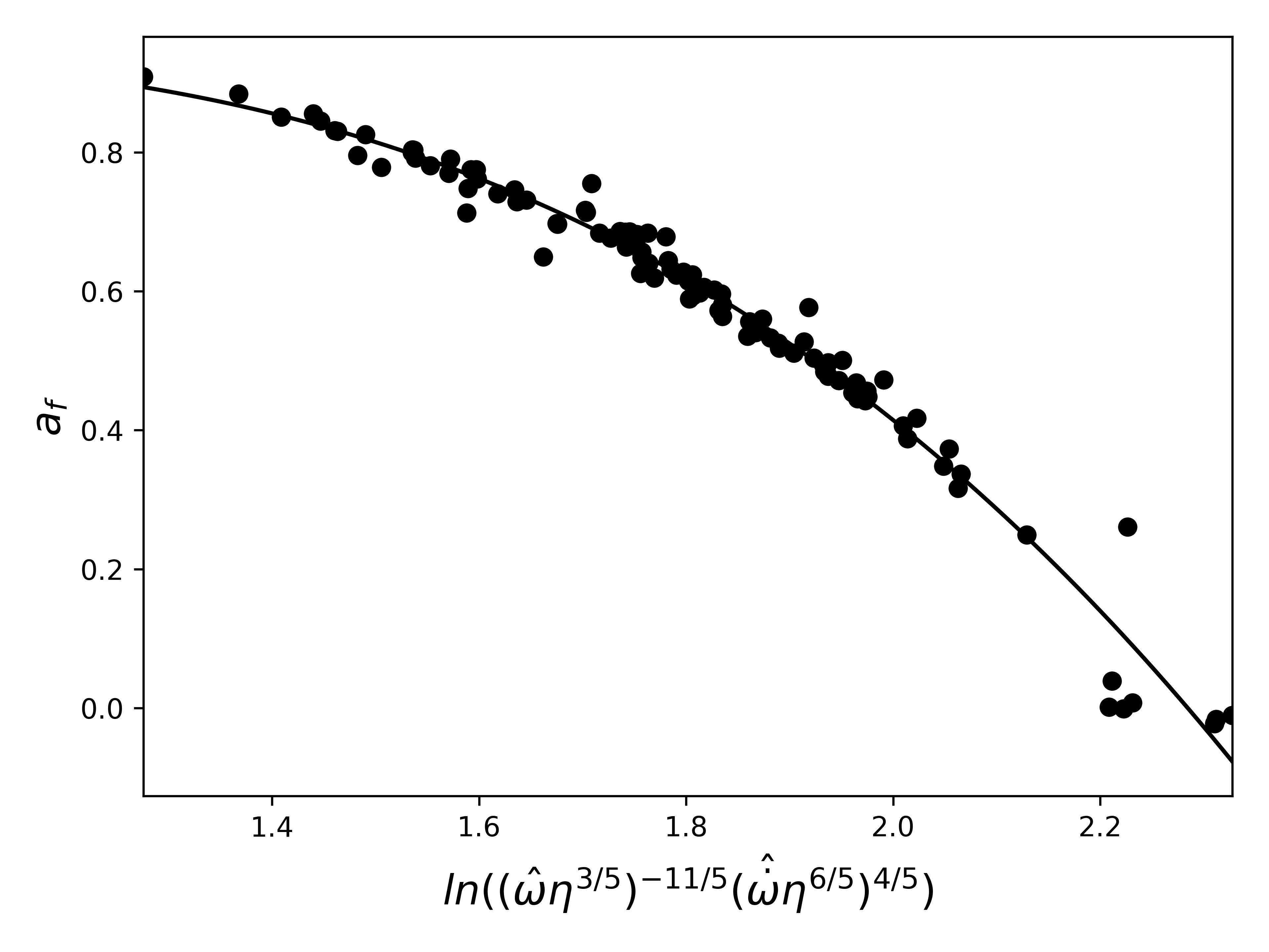
Adopting the same functional form as Healy et.al Healy et al. (2014), we obtain the following best fit relationship
| (6) |
with an average spread of .
III Final Spin
Having found an NR derived relationship relating , , and to , it’s important to study how these values are obtained from real data and how precise this method will be when faced with a detection. is measured by burst searches that fit the frequency evolution of the signal Tiwari et al. (2016). By analyzing the recovered of existing cWB runs, and using the knowledge that the uncertainty scales as 1/signal-to-noise ratio (SNR) Vallisneri (2008), we estimate that the uncertainty in as recovered by cWB is 1.5/SNR. This contributes an additional uncertainty of (126/SNR) % to . For the SNR=100 runs we analyze in this paper, this adds an uncertainty of 1.26% to .
Since GW detector data is noisy, we can’t reliably obtain and directly without first de-noising it. In order to reconstruct a signal out of the noise, we use BayesWave, a search pipeline that relies on modeling the GW as a number of sine Gaussians whose sum results in a coherent GW signal in a detector network Cornish and Littenberg (2015). By using this morphology-agnostic approach, the reconstructed waveform is robust against uncertainties which may be present in templated analyses. The latter model the waveform based on the time orbital evolution of Compact Binary Coalescences and are hence often referred to as CBC analyses Fairhurst and Brady (2008). BayesWave provides an independent, complementary estimate of the waveform morphology, and consequently avoids systematic uncertainty in the frequency evolution which might be present in the best fit CBC waveform Veitch et al. (2015); Messick et al. (2017). In this study we analyze the waveform as reconstructed by BayesWave for the Livingston detector only.
To quantify the expected uncertainty in the remnant spin, we performed a systematic Monte-Carlo study whereby sets of BBH signals with increasing SNR Parzen (2006) were added to stationary Gaussian noise colored with the power spectral density of O1 era LIGO detectors. The underlying waveforms for these “injections” were then recovered using BayesWave. For a SNR of 100, we injected a signal consistent with that of GW150914 in 2000 realizations of Gaussian noise and recovered and for the median waveform of each. The value of was obtained by first calculating the amplitude envelope of the median whitened waveform (using a python implementation of the Hilbert-Huang transform Huang et al. (1998)) and then locating the time at which the amplitude is maximum. Then the median time frequency track, outputted by BayesWave, is used to identify the frequency and the time derivative of the frequency at the given time.
Fig 3 shows the cumulative probability distribution of the estimated for our 2000 injections. The solid black line denotes the median, the solid red line denotes the true final spin, and the dotted lines show the 90% confidence interval, which is =(0.51, 0.77) for SNR of 100.
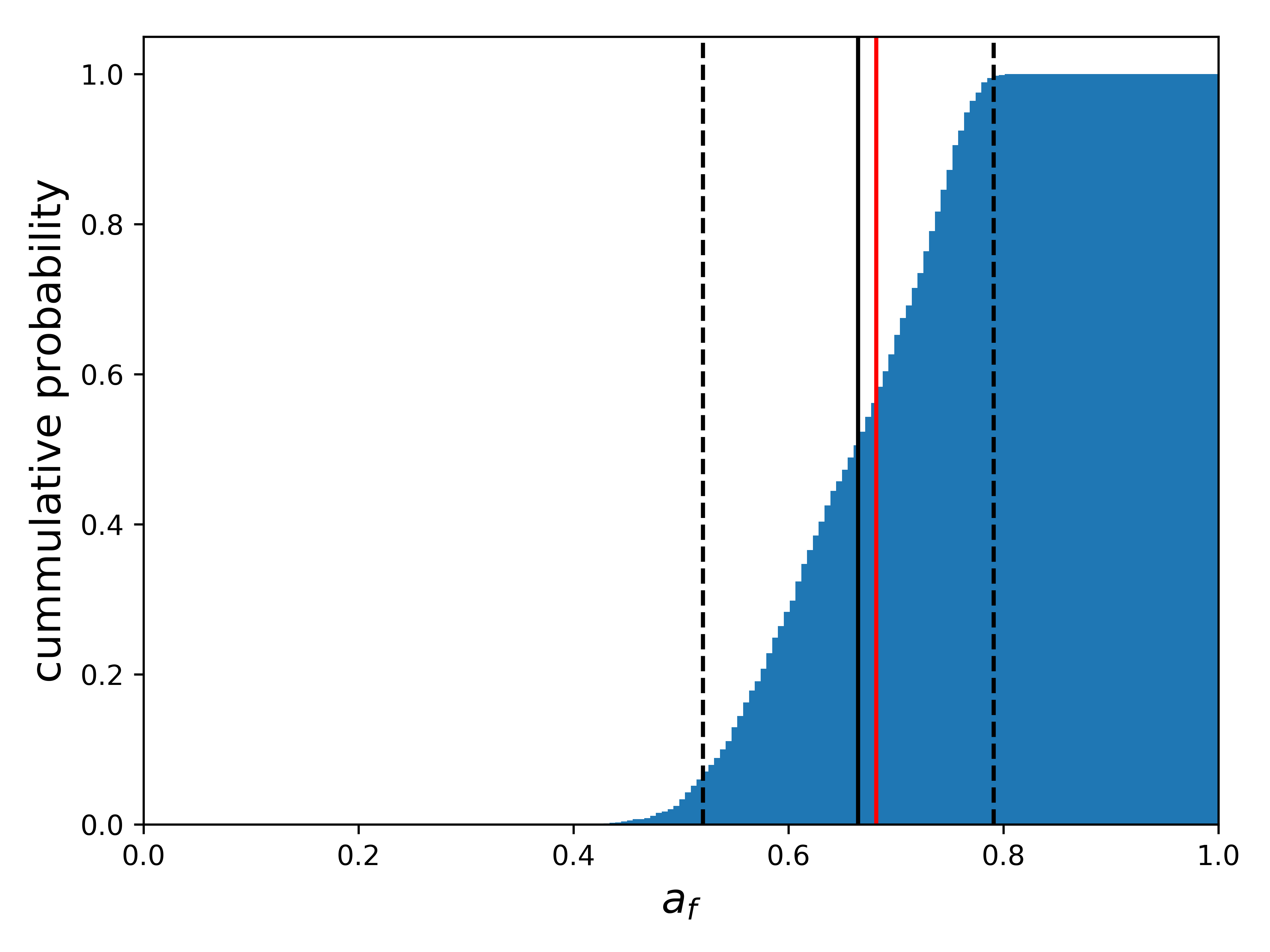
To better understand how this error scales with SNR, we used the same technique just described with 250 injections each for SNRs 40, 60, 80, and 100. The resulting medians and 90% confidence intervals are shown in Table 1.
| SNR | median | lower 90% confidence | upper 90% confidence |
|---|---|---|---|
| 40 | 0.671 | 0.437 | 0.802 |
| 60 | 0.677 | 0.484 | 0.785 |
| 80 | 0.654 | 0.497 | 0.782 |
| 100 | 0.667 | 0.510 | 0.772 |
IV Conclusions
This study finds that the remnant spin is known at the peak amplitude and presents a method of estimating it from the chirp mass, the frequency at maximum amplitude of the strain, and its derivative in an analytic relationship. This allows us to make use of the high SNR at the peak to estimate the final spin before entering the perturbative ringdown regime.
In order to understand the viability of this study as a parameter estimation method, we analyzed the distribution of the remnant spin obtained via recovering the waveform of a GW150914-like signal with increasing SNRs from 40 to 100. We demonstrate that we can reliably place bounds on the spin of the remnant BH using information found near the peak amplitude when the signal is dominated by the , mode.
Our method avoids the usage of BBH templates, instead obtaining and from a BayesWave reconstruction and from cWB. While matched filtering methods likely place a tighter bound on the remnant spin, our alternate approach is not subject to the same systematic biases due to waveform modeling present in the matched filter search. There remain systematic errors due to the fit we are using to determine the final spin from the peak amplitude. In addition, the fitting formula is an interpolation over a discrete set of NR templates and might change if more NR simulations are added to the fit.
Next steps in this study will see the method applied to all the LIGO/VIRGO BBH detections with reasonable BayesWave reconstructions from O1, O2 and, soon, O3. It will also be interesting to see the effect of adding precessing runs to the fit and whether this analysis can be expanded to include higher modes.
Acknowledgements
PL and DS gratefully acknowledge support from the NSF grants PHY-1806580, PHY-1809572, PHY-1550461 and 1333360, XSEDE TG-PHY120016. JCB also acknowledges support from Australian Research Council Discovery Project DP180103155. This research was also supported in part through research cyberinfrastructure resources and services provided by the Partnership for an Advanced Computing Environment (PACE) at the Georgia Institute of Technology. The authors are grateful for computational resources provided by the LIGO Laboratory and supported by National Science Foundation Grants PHY-0757058 and PHY-0823459. We also thank Karan Jani for useful discussions.
References
- Aasi et al. (2015) J. Aasi et al. (LIGO Scientific), Class. Quant. Grav. 32, 074001 (2015), arXiv:1411.4547 [gr-qc] .
- Acernese et al. (2015) F. Acernese et al. (VIRGO), Class. Quant. Grav. 32, 024001 (2015), arXiv:1408.3978 [gr-qc] .
- The LIGO Scientific Collaboration and the Virgo Collaboration (2018) The LIGO Scientific Collaboration and the Virgo Collaboration, arXiv e-prints , arXiv:1811.12907 (2018), 1811.12907 [astro-ph.HE] .
- Collaboration and Collaboration (2017) L. S. Collaboration and V. Collaboration, Phys. Rev. Lett. 119, 161101 (2017).
- The LIGO Scientific Collaboration and The Virgo Collaboration (2018) The LIGO Scientific Collaboration and The Virgo Collaboration, arXiv e-prints , arXiv:1811.12940 (2018), 1811.12940 [astro-ph.HE] .
- Maészàros et al. (2019) P. Maészàros, D. B. Fox, C. Hanna, and K. Murase, (2019), arXiv:1906.10212 [astro-ph.HE] .
- Collaboration and Collaboration (2016) L. S. Collaboration and V. Collaboration, Phys. Rev. Lett. 116, 061102 (2016).
- Vishveshwara (1970) C. V. Vishveshwara, Phys. Rev. D 1, 2870 (1970).
- Press (1971) W. H. Press, ApJ Letters 170, L105 (1971).
- Nollert and Price (1999) H.-P. Nollert and R. H. Price, Journal of Mathematical Physics 40, 980 (1999), arXiv:gr-qc/9810074 [gr-qc] .
- Kokkotas and Schmidt (1999) K. D. Kokkotas and B. G. Schmidt, Living Reviews in Relativity 2, 2 (1999), arXiv:gr-qc/9909058 [gr-qc] .
- Berti et al. (2009) E. Berti, V. Cardoso, and A. O. Starinets, Classical and Quantum Gravity 26, 163001 (2009), arXiv:0905.2975 [gr-qc] .
- Echeverria (1989) F. Echeverria, Phys. Rev. D 40, 3194 (1989).
- Abbott et al. (2009) B. P. Abbott et al. (LIGO Scientific), Phys. Rev. D80, 062001 (2009), arXiv:0905.1654 [gr-qc] .
- Goggin and the LIGO Scientific Collaboration (2006) L. M. Goggin and the LIGO Scientific Collaboration, Classical and Quantum Gravity 23, S709 (2006).
- Berti et al. (2007) E. Berti, J. Cardoso, V. Cardoso, and M. Cavaglia, Phys. Rev. D76, 104044 (2007), arXiv:0707.1202 [gr-qc] .
- Carullo et al. (2019a) G. Carullo, W. Del Pozzo, and J. Veitch, arXiv:1902.07527 (2019a).
- Yang et al. (2017) H. Yang, K. Yagi, J. Blackman, L. Lehner, V. Paschalidis, F. Pretorius, and N. Yunes, Phys. Rev. Lett. 118, 161101 (2017).
- Nakano et al. (2018) H. Nakano, T. Narikawa, K.-i. Oohara, K. Sakai, H.-a. Shinkai, H. Takahashi, T. Tanaka, N. Uchikata, S. Yamamoto, and T. S. Yamamoto, (2018), arXiv:1811.06443 [gr-qc] .
- Cabero et al. (2018) M. Cabero, C. D. Capano, O. Fischer-Birnholtz, B. Krishnan, A. B. Nielsen, A. H. Nitz, and C. M. Biwer, Phys. Rev. D 97, 124069 (2018).
- Dreyer et al. (2004) O. Dreyer, B. J. Kelly, B. Krishnan, L. S. Finn, D. Garrison, and R. Lopez-Aleman, Class. Quant. Grav. 21, 787 (2004), arXiv:gr-qc/0309007 [gr-qc] .
- Berti et al. (2006) E. Berti, V. Cardoso, and C. M. Will, Phys. Rev. D73, 064030 (2006), arXiv:gr-qc/0512160 [gr-qc] .
- Brito et al. (2018) R. Brito, A. Buonanno, and V. Raymond, Phys. Rev. D 98, 084038 (2018).
- Bhagwat et al. (2018) S. Bhagwat, M. Okounkova, S. W. Ballmer, D. A. Brown, M. Giesler, M. A. Scheel, and S. A. Teukolsky, Phys. Rev. D97, 104065 (2018), arXiv:1711.00926 [gr-qc] .
- Carullo et al. (2018) G. Carullo, L. van der Schaaf, L. London, P. T. H. Pang, K. W. Tsang, O. A. Hannuksela, J. Meidam, M. Agathos, A. Samajdar, A. Ghosh, T. G. F. Li, W. Del Pozzo, and C. Van Den Broeck, Phys. Rev. D 98, 104020 (2018).
- Abbott et al. (2016) B. P. Abbott et al. (Virgo, LIGO Scientific), Phys. Rev. Lett. 116, 221101 (2016), [Erratum: Phys. Rev. Lett.121,no.12,129902(2018)], arXiv:1602.03841 [gr-qc] .
- Healy et al. (2014) J. Healy, C. O. Lousto, and Y. Zlochower, Phys. Rev. D90, 104004 (2014), arXiv:1406.7295 [gr-qc] .
- Rezzolla et al. (2008) L. Rezzolla, P. Diener, E. N. Dorband, D. Pollney, C. Reisswig, E. Schnetter, and J. Seiler, Astrophys. J. 674, L29 (2008), arXiv:0710.3345 [gr-qc] .
- Healy and Lousto (2017) J. Healy and C. O. Lousto, PRD 95, 024037 (2017), arXiv:1610.09713 [gr-qc] .
- Jiménez-Forteza et al. (2017) X. Jiménez-Forteza, D. Keitel, S. Husa, M. Hannam, S. Khan, and M. Pürrer, PRD 95, 064024 (2017), arXiv:1611.00332 [gr-qc] .
- Hofmann et al. (2016) F. Hofmann, E. Barausse, and L. Rezzolla, ApJL 825, L19 (2016), arXiv:1605.01938 [gr-qc] .
- Abbott et al. (2019) B. P. Abbott et al. (LIGO Scientific, Virgo), (2019), arXiv:1903.04467 [gr-qc] .
- Ghosh et al. (2018) A. Ghosh, N. K. Johnson-Mcdaniel, A. Ghosh, C. K. Mishra, P. Ajith, W. Del Pozzo, C. P. L. Berry, A. B. Nielsen, and L. London, Class. Quant. Grav. 35, 014002 (2018), arXiv:1704.06784 [gr-qc] .
- Ghosh et al. (2016) A. Ghosh et al., Phys. Rev. D94, 021101 (2016), arXiv:1602.02453 [gr-qc] .
- Carullo et al. (2019b) G. Carullo, G. Riemenschneider, K. W. Tsang, A. Nagar, and W. Del Pozzo, Class. Quant. Grav. 36, 105009 (2019b), arXiv:1811.08744 [gr-qc] .
- Healy et al. (2014) J. Healy, P. Laguna, and D. Shoemaker, Classical and Quantum Gravity 31, 212001 (2014), arXiv:1407.5989 [gr-qc] .
- Buonanno et al. (2007) A. Buonanno, G. B. Cook, and F. Pretorius, Phys. Rev. D75, 124018 (2007), arXiv:gr-qc/0610122 [gr-qc] .
- Kamaretsos et al. (2012) I. Kamaretsos, M. Hannam, and B. S. Sathyaprakash, Phys. Rev. Lett. 109, 141102 (2012).
- Giesler et al. (2019) M. Giesler, M. Isi, M. Scheel, and S. Teukolsky, (2019), arXiv:1903.08284 [gr-qc] .
- Tiwari et al. (2016) V. Tiwari, S. Klimenko, V. Necula, and G. Mitselmakher, Class. Quant. Grav. 33, 01LT01 (2016), arXiv:1510.02426 [astro-ph.IM] .
- Jani et al. (2016) K. Jani, J. Healy, J. A. Clark, L. London, P. Laguna, and D. Shoemaker, Classical and Quantum Gravity 33, 204001 (2016), arXiv:1605.03204 [gr-qc] .
- Herrmann et al. (2007) F. Herrmann, I. Hinder, D. Shoemaker, and P. Laguna, Classical and Quantum Gravity 24, S33 (2007), arXiv:gr-qc/0601026 [gr-qc] .
- Vaishnav et al. (2007) B. Vaishnav, I. Hinder, F. Herrmann, and D. Shoemaker, Phys. Rev. D 76, 084020 (2007), arXiv:0705.3829 [gr-qc] .
- Healy et al. (2009) J. Healy, J. Levin, and D. Shoemaker, Phys. Rev. Lett. 103, 131101 (2009).
- Pekowsky et al. (2013a) L. Pekowsky, R. O’Shaughnessy, J. Healy, and D. Shoemaker, Phys. Rev. D 88, 024040 (2013a).
- Loffler et al. (2012) F. Loffler et al., Class. Quant. Grav. 29, 115001 (2012), arXiv:1111.3344 [gr-qc] .
- Schnetter et al. (2004) E. Schnetter, S. H. Hawley, and I. Hawke, Class. Quant. Grav. 21, 1465 (2004), arXiv:gr-qc/0310042 [gr-qc] .
- Thornburg (2004) J. Thornburg, Class. Quant. Grav. 21, 743 (2004), arXiv:gr-qc/0306056 [gr-qc] .
- Reisswig and Pollney (2011) C. Reisswig and D. Pollney, Class. Quant. Grav. 28, 195015 (2011), arXiv:1006.1632 [gr-qc] .
- Calderón Bustillo et al. (2017) J. Calderón Bustillo, P. Laguna, and D. Shoemaker, Phys. Rev. D95, 104038 (2017), arXiv:1612.02340 [gr-qc] .
- Calderón Bustillo et al. (2016) J. Calderón Bustillo, S. Husa, A. M. Sintes, and M. Pürrer, Phys. Rev. D93, 084019 (2016), arXiv:1511.02060 [gr-qc] .
- Pekowsky et al. (2013b) L. Pekowsky, J. Healy, D. Shoemaker, and P. Laguna, Phys. Rev. D87, 084008 (2013b), arXiv:1210.1891 [gr-qc] .
- Varma and Ajith (2017) V. Varma and P. Ajith, Phys. Rev. D96, 124024 (2017), arXiv:1612.05608 [gr-qc] .
- Vallisneri (2008) M. Vallisneri, Phys. Rev. D77, 042001 (2008), arXiv:gr-qc/0703086 [GR-QC] .
- Cornish and Littenberg (2015) N. J. Cornish and T. B. Littenberg, Class. Quant. Grav. 32, 135012 (2015), arXiv:1410.3835 [gr-qc] .
- Fairhurst and Brady (2008) S. Fairhurst and P. Brady, Class. Quant. Grav. 25, 105002 (2008).
- Veitch et al. (2015) J. Veitch, V. Raymond, B. Farr, W. Farr, P. Graff, S. Vitale, B. Aylott, K. Blackburn, N. Christensen, M. Coughlin, et al., Physical Review D 91, 042003 (2015).
- Messick et al. (2017) C. Messick, K. Blackburn, P. Brady, P. Brockill, K. Cannon, R. Cariou, S. Caudill, S. J. Chamberlin, J. D. E. Creighton, R. Everett, C. Hanna, D. Keppel, R. N. Lang, T. G. F. Li, D. Meacher, A. Nielsen, C. Pankow, S. Privitera, H. Qi, S. Sachdev, L. Sadeghian, L. Singer, E. G. Thomas, L. Wade, M. Wade, A. Weinstein, and K. Wiesner, Phys. Rev. D 95, 042001 (2017), arXiv:1604.04324 [astro-ph.IM] .
- Parzen (2006) E. Parzen, IEEE Trans. Inf. Theor. 9, 127 (2006).
- Huang et al. (1998) N. E. Huang, Z. Shen, S. R. Long, M. C. Wu, H. H. Shih, Q. Zheng, N.-C. Yen, C. C. Tung, and H. H. Liu, Proceedings of the Royal Society of London. Series A: Mathematical, Physical and Engineering Sciences 454, 903 (1998), https://royalsocietypublishing.org/doi/pdf/10.1098/rspa.1998.0193 .