$\alpha$-attractor dark energy in view of next-generation cosmological surveys

Abstract

The $\alpha$-attractor inflationary models are nowadays favored by CMB Planck observations. Their similarity with canonical quintessence models motivates the exploration of a common framework that explains both inflation and dark energy. We study the expected constraints that next-generation cosmological experiments will be able to impose for the dark energy $\alpha$-attractor model. We systematically account for the constraining power of SNIa from WFIRST, BAO from DESI and WFIRST, galaxy clustering and shear from LSST and Stage-4 CMB experiments. We assume a tensor-to-scalar ratio, $10^{-3}<r<10^{-2}$, which permits to explore the wide regime sufficiently close, but distinct, to a cosmological constant, without need of fine tunning the initial value of the field. We find that the combination S4CMB + LSST + SNIa will achieve the best results, improving the FoM by almost an order of magnitude; respect to the S4CMB + BAO + SNIa case. We find this is also true for the FoM of the $w_{0}-w_{a}$ parameters. Therefore, future surveys will be uniquely able to probe models connecting early and late cosmic acceleration.

1 Introduction

The standard model of cosmology relies on two epochs of accelerated expansion. A first inflationary phase in the very early universe leading to a very homogeneous, isotropic and spatially flat with a near scale invariant spectrum of curvature perturbations [1, 2]. The second acceleration era, when dark energy (DE) dominates the energy density in the late universe, is necessary to explain observations of type Ia supernovae (e.g. Refs. [3, 4, 5]), the cosmic microwave background (CMB) (e.g. Refs. [6, 7]) and the large-scale structure (LSS) in the matter distribution (e.g. Ref. [8]). An ambitious observational program aims at elucidating the physics behind inflation and DE.

In this context, the dark-energy $\alpha$-attractor model [9] is one of the models that try to describe both accelerated expansions in a common framework. These models typically have a scalar field in a potential with two plateaus that allow for a slow roll at early times, which produces inflation, and a freezing behavior at late times, that yields a cosmological constant-like expansion [10, 11, 12, 13]. In addition, there are models that would produce dark energy from a symmetry breaking mechanism [14, 15, 16]. However, there are other studies that try to study the connection of the late and early Universe, but focus only on the late time cosmology. Among them there are those describing dark energy as quintessence, which base their Lagrangian on an $\alpha$-attractor model [9, 17, 18, 19, 20], or those which study the relation between them and $f(R)$ gravity, from extensions of the Starobinsky $R^{2}$ gravity [21], as in Refs. [22, 23]. Others, instead, use the $\alpha$-attractors as source of dark matter [24].

During inflation, the $\alpha$-attractors class of models shines as a group of models able to reproduce the observations, which strongly support concave potential models. CMB Planck sets tight constraints on the tensor-to-scalar ratio, $r$, with $r<0.11$ (at $95\%$ CL) and the spectral index, $n_{s}$, with $n_{s}=0.9649\pm 0.0042$ (at $95\%$ CL), favoring slow-roll models with a concave potential ($V(\phi)^{\prime\prime}<0$) [2], as was already anticipated by WMAP results [25]. In this context, the $\alpha$-attractor models are able to give the correct predictions thanks to the fact that, for $N$ e-folds [26],

$$n_{s}=1-2N^{-1}\quad\mbox{ and }\quad r=12\alpha N^{-2}\,,$$ (1.1)

where $\alpha$ is a parameter shared by all models in this class and is present in their Lagrangian, whose canonical expression is given by

$${\mathcal{L}}=\sqrt{-g}\,\left[\frac{1}{2}M_{P}^{2}R-\frac{1}{2}(\partial\phi)^{2}-\alpha f^{2}(x)\right]\ ,$$ (1.2)

where $x=\tanh(\phi/\sqrt{6\alpha})$. The fact that their Lagrangian is the same as the one for canonical quintessence dark energy models is exploited to connect both inflation and dark energy with the same scalar field.

The $\alpha$-attractor models are connected with fundamental theories with various fields with local conformal (i.e. rescaling) invariance. This symmetry allows to rewrite the original Lagrangian as a single-field one [26, 27],

$${\mathcal{L}}=\sqrt{-g}\,\left[\frac{1}{2}M_{P}^{2}R-\frac{\alpha}{(1-\varphi^{2}/6)^{2}}\,\frac{1}{2}(\partial\varphi)^{2}-\alpha f^{2}\left(\frac{\varphi}{\sqrt{6}}\right)\right]\ .$$ (1.3)

Here, $g$ is the metric and $R$ the Ricci scalar, $M_{P}$ is the Planck mass, and $\alpha f^{2}$ is the potential function dependent on the field $\varphi$ which is measured in $M_{P}$ units. The second order pole in the kinetic term is the reason behind the common predictions for $n_{s}$ and $r$ (Eq. 1.1). Finally, in order to obtain its canonical version, one needs to define $\phi=\sqrt{6\alpha}\,\operatorname{arctanh}(\varphi/\sqrt{6})$. In this way, one also pushes the boundaries of the connected region ($\varphi\in(-\sqrt{6},\sqrt{6})$) to infinity ($\phi\in(-\infty,\infty)$).

In this paper, we will extend the previous work of Ref. [19] that studied the phenomenology and the observational constraints of a generalized $\alpha$-attractor dark energy model, based on Starobinsky $R^{2}$ inflationary Lagrangian [21]. It was shown that the generalized Starobinsky-model had an infinite $\Lambda$CDM-like region which made that, imposing only late time observational constraints (and a true model close to $\Lambda$CDM), one could only have lower bounds on the initial position of the field and $\alpha$ and the requirement on the exponents of being of the same order, so that the field slow rolls.

We will systematically study how future observations will affect the constraints on the model’s parameters. Next spectroscopic experiments generation will reduce the relative error on the angular diameter distance and the Hubble parameter to order of a few percents, while deepening up to $z\sim 3$ [28, 29]. Baryonic Acoustic Oscillations (BAO) measurements will also significantly improve their accuracy, what will be reflected on the parameter constraints [19]. On the other hand, Stage 4-CMB experiments are expected to measure the tensor-to-scalar ratio to order $\sigma(r)\sim 0.001$ [30]. Lowering the $r$ upper-bound below $\sim 0.01$ might be able to constrain $\alpha$ through Eq. 1.1 and, in turn, the initial value of the field. Finally, from the Large Synoptic Survey Telescope [31], a photometric experiment, we will take into account their predictions for galaxy clustering and shear measurements, which will effectively constrain cosmological parameters by means of precise measurements of the matter power spectrum at different redshifts.

It is important to note that some of these next-generation experiments will overlap, allowing to beat cosmic variance when cross-correlations are taken into account [32]. In order to take advantage of this piece of information, we will use the multi-tracer formalism as described in Ref. [33], which is reviewed in Section 4.

In Section 2, we will introduce the $\alpha$-attractor dark energy model and summarize its properties. In Section 3, we will briefly summarize the models used to describe each observational probe that enter our forecast: Stage-4 CMB experiments, the Large Synoptic Survey Telescope [31], DESI [28] and WFIRST [6]. In Section 4, we will review the multi-tracer Fisher formalism and the computational tools that carry out the computations. In Section 5, the forecasted constraints will be shown and analyzed. Finally, in section 7, we will conclude.

2 The generalized $\alpha$-attractor model

The generalized $\alpha$-attractor model was first proposed in Ref. [9] and further studied in Refs. [17, 19]. It generalizes the Starobinsky inflationary model [21], freeing the potential’s exponents and amplitude:

$$V(x)=\alpha c^{2}\,\frac{x^{p}}{(1+x)^{2n}}=\alpha c^{2}2^{-2n}(1-y)^{p}(1+y)^{2n-p}\ ,$$ (2.1)

where $c$, $p$, $n$ are constant parameters, $x=\tanh(\phi/\sqrt{6\alpha})$ and $y\equiv e^{-2\phi/\sqrt{6\alpha}}$. The Starobinsky model is obtained with $\alpha=1$, $p=2$, $n=1$ [34, 35, 36], in natural units, i.e. reduced Planck mass $M_{P}=1$ and speed of light, $c=1$. We assume a flat Universe as a consequence of inflation.

In this section, we will summarize the properties of this model, already studied in Ref. [9, 19]. We will use the scaled field variable, $\psi\equiv\phi/\sqrt{6}$, introduced in Ref. [19], as it better reflects what is the determining quantity in $V(x)$. Let us list them bellow:

• The potential Eq. 2.1 has two limits – it has a power law regime at low $\psi$ and a plateau at large $\psi$ [9]:

  $$V(|\psi|\ll\sqrt{6}) \approx \alpha c^{2}6^{-p/2}\,\psi^{p}\ ,$$ (2.2)

  $$V(\psi\gg\sqrt{6}) \approx \alpha c^{2}\,2^{-2n}\,\left[1-2(p-n)\,e^{-2\psi/\sqrt{6}}\right]$$ (2.3)

  $$\xrightarrow[\psi\to\infty]{} \frac{\alpha c^{2}}{2^{2n}}\ .$$ (2.4)

• Viable models are of the thawing class and $\Delta\psi\equiv\psi_{0}-\psi_{i}$ (the field excursion, i.e. the difference between its initial, $\psi_{i}$ and today’s, $\psi_{0}$, values), can be approximated as $\Delta\psi\sim\sqrt{1+w_{0}}/\sqrt{\alpha}$. In addition, it can be shown that $1+w_{0}\sim 1/\alpha$, yielding $\Delta\psi\sim 1/\alpha$ [19].

• If $n<p$, the field always decreases [9] and its velocity is inversely related to its initial value ($\psi_{ini}$). Also, $p$ determine the transition regime slope [19].

• If $n>p$, it has a maximum located at $x_{max}=p/(2n-p)$ [9], whose height for viable models is controlled by $n$ and the transition regime slope by $p-n$. Around the inflection points the field evolution is fast [19].

The observational constraints obtained with Planck 2015 [37], BAO from BOSS DR12 [8] and supernovae (through an $E(z)$ estimate with Pantheon compressed sample) [38] show that large $\alpha$ and $\psi_{ini}$ are favored as they make the field move slowly. For the same reason, $p\sim n$ is also preferred. Finally, despite of having viable tachyonic solutions, this model would not cause dark energy to cluster significantly, since dark energy perturbation do not have enough time to grow appreciably [19].

Note that the lower boundary of $\psi_{ini}$ depends on the maximum value accessible for $\alpha$, since the total evolution of the field is inversely related to $\alpha$ (second item of previous list). As a consequence, constraining $\alpha$ through Eq. 1.1 and $n_{s}$ and $r$ measurements could significantly improve the previous result of Ref. [19], cutting out a big portion of the available space for $\psi_{ini}$. Quantitatively,

$$\alpha=\frac{r}{3(1-n_{s})^{2}}\,,$$ (2.5)

so that if Stage 4-CMB experiments measured $r<0.01$, $\alpha\lesssim 3.5$, which would highly constrain the initial position of the field, restricting its values to positions close to the plateau or the maximum, where the field slow-rolls. It would be even more dramatic if $r\sim 10^{-3}$ (exhausting the intended minimum uncertainty [30]), as $\alpha\sim 0.35$. However, if $r$ remained close to its upper bound value of Planck 2018 results ($r\sim 0.1$) [2], $\alpha\sim 38$. Then, the available space for $\psi_{ini}$ would expand towards values closer to the potential minimum and the inflection points, thanks to the friction $\alpha$ causes.

In this work, we will study the case with $r\lesssim 0.01$, which will allow to explore the regimes in which the model is both close and different to a cosmological constant. The mild upper bound in $\alpha$ ($\alpha\lesssim 3.5$) will restrict $\psi_{ini}$ to values where the field does not roll down fast, but far enough to the plateau and maximum, allowing a mild evolution. A tighter constraint, as that set by the most precise expected measurement of $r$, $r\sim 10^{-3}$ [30], fixes $\alpha\sim 0.35$, pushing the equation of state towards $w\sim-1$ to avoid the parts of the potential where the field would move fast and yield inviable models, letting alone the maximum (instable), the plateau and their closest points. In addition, we choose to avoid the high $\alpha$ regime (i.e. high $r$) as it was shown to be unbounded by current data [19]. The only hope of constraining the parameter space relies on finding new data that favors a model sufficiently distinct to $\Lambda$CDM and, in that case, our choice of $r\lesssim 0.01$ ($\alpha\lesssim 3.5$) is broad enough to account for a wide range of cosmologies that deviate from $\Lambda$CDM.

3 Observational probes

A cohort of next-generation cosmology experiments will collect an unprecedented amount of data during the next decade, which will allow us to vastly improve our understanding of cosmology. Our forecasts will include two experiments modelled after two of the most promising facilities: CMB Stage-4 and the Large Synoptic Survey Telescope (LSST). The assumptions made to describe these datasets will be described here.

3.1 CMB Stage 4

Third-generation CMB experiments, such as ACTPol [39], SPT-3G [40], BICEP2/Keck [41] or Simons Array [42] will be progressively upgraded to an Stage 4 experiment, increasing the number of detectors, frequency channels, and sky coverage, allowing us to cover around $40\%$ of the sky, with a white-noise level $\sigma_{T}\sim 1\mu K$-arcmin in temperature [30].

S4 will measure primordial CMB temperature and polarization anisotropies as well as the reconstructed CMB lensing convergence, among other secondary anisotropies. These measurements will be limited in resolution by the beam size. We assume a Gaussian beam with a full width at half maximum $\theta_{FWHM}=3$ arcmin. The corresponding noise power spectrum, assuming white noise, is given by

$$N_{\ell}^{x}=\sigma_{x}^{2}\exp\left[\ell(\ell+1)\theta^{2}_{FWHM}/8\log 2\right]\,,$$ (3.1)

where $x$ stands for temperature ($T$) or polarization maps ($E$) and $\sigma^{2}_{x}$ is in units of $\mathrm{}[\mu K^{2}{\rm sr}]$ (we assume $\sigma_{E}=\sigma_{T}\sqrt{2}$). At large scales, statistical and systematic uncertainties, associated to ground-based facilities such as atmospheric contamination dominate, and therefore we discard multipoles $l<30$ and use the Planck noise levels in this regime [43] (corresponding to $\sigma_{T}\simeq 30\,\mu{\rm K}$-arcmin. Furthermore, given the contamination in the temperature power spectrum by astrophysical foregrounds, we choose different scale cuts for polarization ($\ell_{\rm max}=5000$) and temperature ($\ell_{\rm max}=3000$) multipoles.

Lensing noise is obtained by quadratic combinations of the CMB maps [44] and estimating the reconstruction noise with the minimum variance weighting, by combinations of the $TT\,,TE\,,TB\,,EB$ and $EE$ individual estimators. This technique significantly reduces the noise of individual estimators which are noise limited at high-$\ell$ [45]. We include CMB lensing information in the range $30<\ell<3000$.

3.2 The Large Synoptic Survey Telescope

The Large Synoptic Survey Telescope (LSST) is a photometric Stage 4 experiment that will cover around $20,000\,{\rm deg}^{2}$ and reach a limit magnitude $r\sim 27$ [31]. Photometric catalogs are dense and deep, which make them excellent for weak lensing studies and multi-probe analyses, where one does not need high accuracy on the spatial distribution of the tracers or clustering statistics at small scales.

Photometric surveys infer the individual galaxies redshifts from their fluxes in a few broad frequency bands and, as a consequence, have large uncertainties in the radial clustering pattern. This procedure, will allow LSST to obtain constraints from different sources: tomographic galaxy clustering and cosmic shear, galaxy cluster counts, SN Ia and strong lenses. Among these, the combination of galaxy clustering and cosmic shear is the most promising source of information for LSST when combined with measurements of the distance-redshift relation (through e.g. supernovae or baryon acoustic oscillations). We will follow Ref. [46] in the modelling of both tracers.

• Galaxy clustering. For galaxy clustering, the most relevant observable is the shape of the angular power spectrum or the two-point correlation function of the galaxy distribution. In tomographic clustering, we divide the galaxy sample in redshift bins and compute the auto- and cross-correlation functions between them. In order to simplify the analysis, we assume that galaxies can be grouped in two different categories – red galaxies (early-type, elliptical and high-bias) and blue galaxies (late-type, spiral and low-bias). This is just an approximation, since red spiral galaxies exist, for example, but it is based on the strong bimodality of the galaxy color space [47]. For instance, red galaxies are less abundant, but show strong features in their spectra that allow to extract more accurate photo-$z$ distributions. Furthermore, they also show a higher clustering amplitude (i.e. they have a larger galaxy bias) than their blue counterparts. In addition tho these two classes of galaxies, we group together all galaxies whose magnitude is above $r\simeq 25.3$, which correspond to the so-called ‘gold sample’ of LSST [31], and will be used as the galaxy shear sample for weak lensing. In galaxy clustering, the main source of statistical noise is shot noise and, following Ref. [46], the noise power spectra is given by

  $$N_{l}^{ij}=\frac{\delta_{ij}}{n^{i}}\,$$ (3.2)

  where $n^{i}$ is the angular number density of galaxies in the $i$-th tomographic bin, characterized by its window function $w^{i}(z)$,

  $$n^{i}=\int_{0}^{\infty}dz\,\bar{N}(z)w^{i}(z)\,.$$ (3.3)

  We assume, Gaussian photo-$z$ distributions ($p(z_{p}|z)$), for which the window function is

  $$w^{i}(z) = \int_{z_{0}^{i}}^{z_{f}^{i}}dz_{p}\,p(z_{p}|z)$$ (3.4)

  $$= \frac{1}{2}\left[\mbox{erf}\left(\frac{z-z_{0}^{i}}{\sqrt{2}\sigma_{z}}\right)-\mbox{erf}\left(\frac{z-z_{f}^{i}}{\sqrt{2}\sigma_{z}}\right)\right]\,.$$ (3.5)

  Here $\sigma_{z}$ is the Gaussian photo-$z$ standard deviation, which we parametrize as $\sigma_{z}(z)=\sigma_{0}(1+z)$. We use $\sigma_{0}=0.02$ for red galaxies and $\sigma_{0}=0.05$ for the blue and gold samples (red galaxies have usually more precise photo-$z$ due to their stronger spectral features). Finally, the list of initial and final redshifts for each redshift bin can be found in Table 1, and the galaxy distributions in Fig. 1. Note that the redshift spacing was chosen such that the width of each bin is equal to 3 times the photo-$z$ uncertainty at the center of the bin. This is a compromise between the need to sample the redshift range sufficiently well, and avoiding strong correlations between different bins due to their overlap.

  

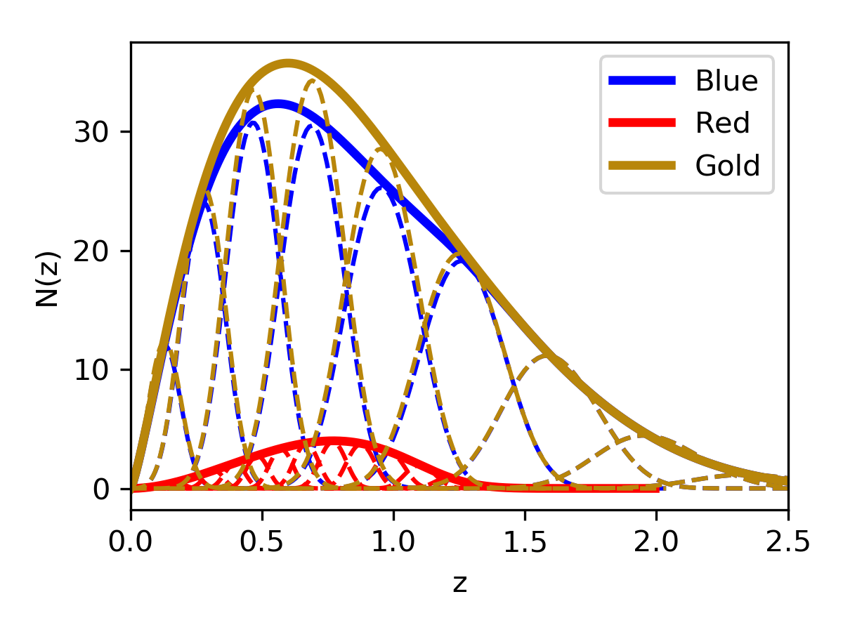
  Figure 1: Galaxy density distributions for red, blue and gold samples of LSST. Dashed lines show the windows functions ($W^{i}\propto\bar{N}(z)w^{i}(z)$) for each redshift bin.

  The main source of uncertainty for galaxy clustering is the relation between the galaxy and matter overdensities. On sufficiently large scales, this relation is assumed to be linear, and the proportionality constant is the so-called galaxy bias $b$ [48]. We use a model for the bias of red and blue galaxies as

  $$b_{red}(z)=1+z,\qquad b_{blue}=1+0.84z\,.$$ (3.6)

  This is motivated by simulations [49] and observations [50], and takes into account the stronger clustering properties of red galaxies.

  Given that the linear bias parametrization breaks on small scales, our scale cuts for galaxy clustering need to be more conservative. We will define it in a redshift dependent manner as $\ell_{\rm max}(\overline{z})=\chi(\overline{z})k_{\rm max}$, where $\overline{z}$ is the mean redshift of the redshift bin, $\chi$ is the radial comoving distance and $k_{\rm max}$ is the threshold comoving scale, which we choose to be $k_{\rm max}=0.2h\,\mathrm{Mpc^{-1}}$. This is the scale up to which a good estimate of the covariance matrix of the matter power spectrum in the quasi-linear regime can be made at $z=0$ [51].

  Sample	Redshift bin edges
  Blue (cl)	[0, 0.16, 0.35, 0.57, 0.82, 1.12, 1.46, 1.86, 2.33]
  Red (cl) &	[0, 0.06, 0.13, 0.20, 0.27, 0.35, 0.43,
  Gold (sh)	[0.52, 0.62, 0.72, 0.82, 0.94, 1.1, 1.2, 1.3]

  Table 1: Redshift bin edges for the angular galaxy density distribution of each sample. cl $\equiv$ clustering; sh $\equiv$ shear. Refer to appendix B.4.2 in Ref [46] for details on the distributions.

  As a final remark, we will neglect the effect of magnification bias, given the small effect it has on the final constraints [52].

• Galaxy shear. Weak lensing is an unbiased estimator of the projected matter perturbations, and is quantified by correlating the projected ellipticities of galaxies. The noise power spectrum is directly proportional to the variance of the intrinsic galaxy ellipticities, and inversely to the angular projected galaxy number density; i.e. $N_{l}^{ij}=\delta_{ij}\sigma_{\gamma}^{2}/n^{i}$. Here, $\sigma_{\gamma}$ includes both the dispersion of the intrinsic galaxy ellipticities and the measurements uncertainties, and is set to $\sigma_{\gamma}=0.28$ [31]. We marginalize over shape measurement systematics in the form of a free multiplicative bias parameter for each reshift bin. Other sources of systematic uncertainty, such as intrinsic alignment, shape-measurement systematics or baryonic uncertainties will be neglected. We expect their effect on the constraints on the parameter space of the $\alpha$-attractor dark energy model to be negligible compared to other sources of systematic uncertainties, particularly the multiplicative bias. We will however impose a scale cut $\ell\leq 2000$ to avoid uncertainties associated with the modelling of baryonic effects in the matter power spectrum [53, 54, 55, 56, 57, 58, 59]. The redshift bins for the gold sample used for weak lensing are given in Table 1

Tracer	Noise contribution
S4CMB	$N_{l}^{x}=\sigma_{x}^{2}\exp\left[l(l+1)\theta^{2}_{FWHM}/8\log 2\right]$ ,
gal. cl.	$N_{l}^{ij}=\delta_{ij}/n^{i}n^{j}$
gal. sh.	$N_{l}^{i}=\sigma_{\gamma}^{2}/N_{\Omega}^{i}$

Table 2: Noise contribution to the power spectra for LSST measurements. For S4CMB experiments, the noise level $\sigma_{x}=\sigma_{T},\,\sigma_{E}$, where $\sigma_{E}/\sqrt{2}=\sigma_{T}\sim 1\mu K$-arcmin and $\Theta_{FWHM}=\mathrm{3}[arcmin]$. For galaxy clustering (gal. cl.), $\delta_{ij}$ is the identity matrix and $n^{i}$ is the galaxy number in the z-bin $i$, given by Eq. 3.3. For galaxy shear (gal. sh.), the variance of the intrinsic galaxy ellipticities, $\sigma_{\gamma}=0.28$ and $N^{i}_{\Omega}$ is the angular galaxy number density of z-bin $i$.

3.3 Spectroscopic Surveys: DESI and WFIRST

Spectroscopic surveys are especially aimed to study phenomena at smaller scales, like BAO and redshift-space distortions. The high redshift resolution of spectroscopic surveys makes a tomographic analysis as described in the previous section computationally intractable and inefficient. The standard analysis studying the multipoles of the 3D galaxy power spectrum is however not easy to incorporate into our forecasting formalism, in terms of fully characterizing the correlations with overlapping tomographic data.

Instead, we will directly incorporate the BAO forecasts for DESI [28] and WFIRST [6, 29], using the error estimates summarized in Table 3. The errors are given on the angular diameter distance ($D_{A}=(1+z)^{-1}\int_{0}^{z}dz^{\prime}H^{-1}(z^{\prime})$) and Hubble parameter ($H(z)$).

BAO error predictions
DESI			WFIRST
$z$	$\frac{\sigma_{D_{A}/s}}{D_{A}/s}(\%)$	$\frac{\sigma_{Hs}}{Hs}(\%)$	$z$	$\frac{\sigma_{D_{A}/s}}{D_{A}/s}(\%)$	$\frac{\sigma_{Hs}}{Hs}(\%)$
0.05	6.12	12.10	1.05	1.51	2.72
0.15	2.35	4.66	1.15	1.43	2.56
0.25	1.51	2.97	1.25	1.35	2.42
0.35	1.32	2.44	1.35	1.29	2.30
0.45	2.39	3.69	1.45	1.24	2.21
0.65	0.82	1.50	1.55	1.23	2.16
0.75	0.69	1.27	1.65	1.25	2.15
0.85	0.69	1.22	1.75	1.28	2.16
0.95	0.73	1.22	1.85	1.33	2.19
1.05	0.89	1.37	1.95	1.41	2.27
1.15	0.94	1.39	2.05	2.51	3.52
1.25	0.96	1.39	2.15	2.60	3.62
1.35	1.50	2.02	2.25	2.74	3.78
1.45	1.59	2.13	2.35	3.02	4.09
1.55	1.90	2.52	2.45	3.38	4.52
1.65	2.88	3.80	2.55	3.87	5.11
1.75	4.64	6.30	2.65	4.52	5.90
1.85	4.71	6.39	2.75	5.41	6.99

Table 3: WFIRST and DESI BAO errors. Respectively, they have been taken from Table VII in Ref. [29] and Tables 2.3 and 2.5 of Ref. [28]. The early-time BAO error predictions from Ly-$\alpha$ and quasars (QSO) have been omitted as they are above the $H$ and $D_{A}$ partial derivatives (see Fig. 3) values, having little contribution to the total Fisher matrix.

DESI [28] will cover $\sim 14000\,\mathrm{deg^{2}}$ from the North Hemisphere and target Luminous Red Galaxies (LRGs), Emission Line Galaxies (ELGs) and quasars. Their BAO $D_{A}$ and $H$ error estimations cover 18 redshifts, uniformly distributed in the redshift range $0.05\leq z\leq 1.85$. The details of their forecast analysis can be found in Ref. [28]. On the other hand, WFIRST will measure redshifts for $\sim 2.6\times 10^{7}$ galaxies over $\sim 2000\,\mathrm{deg^{2}}$. Their forecast assumed the galaxy number densities from from Ref. [6]. We use forecast errors on the BAO parameters over 18 redshift bins, uniformly distributed in $1.05\leq z\leq 2.75$. Additionally, WFIRST will also be able to measure the expansion of the Universe through type Ia supernovae. We will include this probe through the forecast for $E(z)=H(z)/H(0)$ from Ref. [38] (see Table 4), the same way this was done in Ref. [19]. We will neglect correlations between different redshifts as this effect is negligible in comparison with the constraining power of the other experiments. The predictions for $E(z)$ were obtained from a simulation based on Ref. [60], plus an external sample at $z<0.1$. The predictions for $E(z)$ for WFIRST are based in simulations done by Ref. [60] for WFIRST, where the systematic errors in the adopted model fall below the statistical errors. The number of supernovae in each redshift bin is shown in Table 5.

WFIRST SN Ia
$E(z)$ predictions
$z$	$\sigma(E(z))(\%)$
0.07	1.3
0.2	1.1
0.35	1.5
0.6	1.5
0.8	2.0
1.0	2.3
1.3	2.6
1.7	3.4
2.5	8.9

Table 4: $E(z)=H(z)/H(0)$ estimated relative errors from WFIRST SN Ia. Values have been taken from Table 7 of Ref. [38], based on Ref. [60] simulations plus an external sample at $z<0.1$.

$z\in$	SN
$[0,0.1]$	800
$[0.1,0.4]$	557
$[0.4,0.8]$	4807
$[0.8,1.7]$	5892

Table 5: Redshift bins and number of supernovae obtained in a realistic simulation of the Imaging All-z observational strategy [60], used in Ref [38] to forecast the uncertainties on $E(z)$. The first 800 SN are assumed to be obtained from a different experiment.

4 Fisher formalism

This section summarizes the Fisher formalism introduced in Ref. [33]. Each projected probe (CMB primary and lensing, photometric galaxy clustering and cosmic shear) labelled as $a$ is composed of a number of sky maps $N^{a}_{\rm maps}$, which can be fully described by their harmonic coefficients ($a_{\ell m}^{a\,,i}$, $i\in[0,N^{a}_{\rm maps}]$). They can be grouped into a vector ${\bf a}_{\ell m}$, the covariance matrix of which is the power spectrum::

$$\langle{\bf a}_{\ell m}{\bf a}_{\ell^{\prime}m^{\prime}}^{\dagger}\rangle=\delta_{\ell\ell^{\prime}}\delta_{mm^{\prime}}{\sf C}_{l}\,.$$ (4.1)

Under the assumption of being Gaussian distributed, the likelihood is given by

$$-2\log L=\sum_{\ell_{\rm min}}^{\ell_{\rm max}}\sum_{m=-\ell}^{m=\ell}\left[{\bf a}^{\dagger}_{\ell m}{\sf C}_{\ell}^{-1}{\bf a}_{\ell m}+\log(\det(2\pi{\sf C}_{\ell}))\right]\,,$$ (4.2)

which can be expanded around the maximum in order to find the Fisher matrix

$$F_{\mu\nu}=\sum_{\ell=\ell_{\rm min}}^{\ell_{\rm max}}f_{\rm sky}\frac{2\ell+1}{2}\mbox{tr}\left(\partial_{\mu}C_{\ell}C_{\ell}^{-1}\partial_{\nu}C_{\ell}C_{\ell}^{-1}\right).$$ (4.3)

The covariance matrix of the parameters $\theta$ can then be obtained by inverting $F$. In the previous equation, $\partial_{\mu}$ is the partial derivative respect to the parameter $\theta_{\mu}$ and $f_{sky}$ is the sky fraction covered by the considered probes.

Furthermore, we will assume that noise and cosmological signal are uncorrelated in the observed anisotropies, i.e. given ${\bf a}_{\ell m}={\bf s}_{\ell m}+{\bf n}_{\ell m}$, ${\sf C}_{\ell}={\sf C}_{\ell}^{S}+{\sf C}_{\ell}^{N}=\langle{\bf s}_{\ell m}{\bf s}_{\ell m}^{\dagger}\rangle+\langle{\bf n}_{\ell m}{\bf n}_{\ell m}^{\dagger}\rangle$, where ${\sf C}^{S}_{\ell}$ and ${\sf C}^{N}_{\ell}$ are the signal and noise power spectra.

The Fisher matrix with DESI and WFIRST probes will be computed as

$$F_{\mu\nu}=\sum_{i}\frac{\partial_{\mu}q_{i}\partial_{\nu}q_{i}}{\sigma_{i}^{2}},$$ (4.4)

where $q_{i}$ is the measurement of a given quantity $q$ (which stands for $D_{A}(z)$, or $E(z)$) in the $i$-th redshift bin, and $\sigma_{i}^{2}$ is the forecasted error on that quantity. This Fisher matrix is added to the one computed for CMB and photometric survey data. This ignores possible correlations between both sets of observables. We do not expect our results to be very sensitive to this assumption.

Finally, all partial derivatives with respect to $\theta_{\mu}$ will be computed via finite central differences,

$$\partial_{\mu}f=\frac{f(\theta_{\mu}+\delta\theta_{\mu})-f(\theta_{\mu}-\delta\theta_{\mu})}{2\delta\theta_{\mu}}+O(\delta\theta^{3}).$$ (4.5)

In addition, the power spectra, ${\sf C}_{\ell}^{S}$, will be obtained using hi_class [61], a modified version of CLASS [62] that incorporates Horndeski models [63] without assuming the quasi-static approximation, which ensures results are valid at scales larger than the sound horizon [64]. Finally, we will use the Limber approximation [65] in the full range of scales. The software used to combine all these ingredients is available online.

5 Results

The next generation of data, despite its increase on accuracy, will fail to fully constrain the generalized $\alpha$-attractor model, as present observations did, if they continue preferring a $\Lambda$CDM background evolution. One must recall that this model has an infinite region of the parameter space that is indistinguishable from $\Lambda$CDM, corresponding to large $\alpha$ (acts as a friction to the field motion) or having $\psi_{ini}$ on the plateau (or, with more fine tunning, close to a maximum) [19].

We will investigate the parameter space that lies $1\sigma$ off the best fit result of Ref. [19], which is able to differentiate from a cosmological constant. Current observations prefer the cosmological constant-like regime, which correspond to an unbounded region on the parameter space [19]. Therefore, as we said before, if future observations were to continue favoring $\Lambda$CDM, they would not be able to constrain the parameter space. At best, they will be able to rise the lower bounds for $\alpha$ and $\psi_{ini}$. As a consequence, the only hope of finding tight constraints relies on new data that favors models slightly different (they still have to be compatible with current observations, at their level of accuracy) to $\Lambda$CDM. This regime correspond to the parameters $1\sigma$ off the best-fit of Ref. [19].

The cosmological parameters have been chosen as in Table 3 of Ref. [19], i.e. $\Omega_{cdm}h^{2}=0.1183$, $\Omega_{b}h^{2}=0.02221$, $h=0.682$, $10^{9}A_{s}=2.14$, $n_{s}=0.9649$, $\tau_{reio}=$ = 0.067. For the $\alpha$-attractor parameters, we study two distinct cases, corresponding to models with and without a maximum ($p\geq n$ and $p<n$, respectively). In the first case, the $1\sigma$-off parameters are $\{\psi_{ini},\,\alpha,\,p,\,n\}=\{1.5,\,2,\,2,\,1\}$. In the second case, we choose $\{\alpha,p,n\}=\{2,2,3.5\}$ and we study two further options for $\psi_{ini}$: $0.8$ and $1.4$. This corresponds to the cases with $\psi_{ini}$ smaller and larger than $\psi_{max}=1.04$ (see Fig. 2). A summary of the fiducial models and constraints can be found in Table 6. In next sections, we will discuss them in detail. The $c$ parameter, which fixes the potential amplitude, is fixed via the Friedman equation ($1=\sum_{i}\Omega_{i}$).

Pars.	$\psi_{ini}$	$\alpha$	$p$	$n$	FoM	$\mbox{FoM}_{\mbox{\scriptsize CPL}}$
Fid (no max).	1.5	2	2	1	$-$	$-$
$\sigma$	$\lesssim 1$	0.5	$\lesssim 1$	$\lesssim 1$	$\sim 10$	$10^{3}$
Fid ($\psi_{ini}<\psi_{max}$).	0.8	2	2	3.5	$-$	$-$
$\sigma$	0.2	$\sim 0.5$	0.4	1	$\sim 100$	$10^{2}$
Fid ($\psi_{ini}>\psi_{max}$).	1.4	2	2	3.5	$-$	$-$
$\sigma$	2	$\sim 1$	2	2	$\sim 1$	$10^{4}$

Table 6: Fiducial values and predicted constraints using all probes. Recall that $\psi_{max}=1.04$. The results with a ’$\sim$’ sign mean that little changes on the numerical derivative yield changes on the first significant digit. This is consequence of the strong correlations between the model parameters. $\mbox{FoM}\equiv\mbox{FoM}(\psi_{ini},\,\alpha,\,p,\,n)$ and $\mbox{FoM}_{\mbox{CPL}}\equiv\mbox{FoM}(w_{0},\,w_{a})$. The potential shape when $\psi_{ini}<\psi_{max}$ allows for a larger variety of evolutions and, therefore, of $w_{0}-w_{a}$ values. This causes a greater $\mbox{FoM}_{\mbox{CPL}}$ than in the other cases.

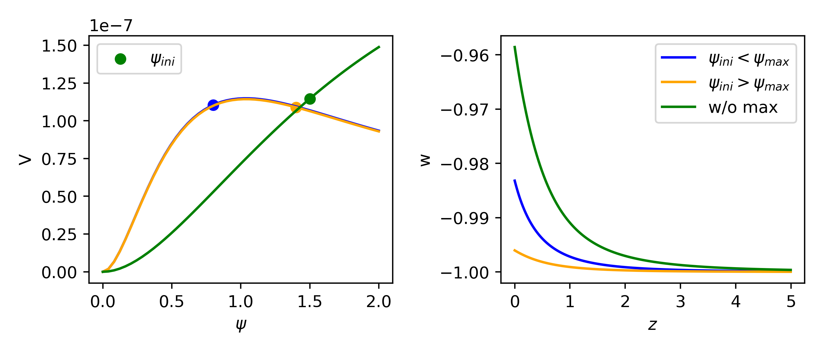
Figure 2: Fiducial potentials ($V$) and equations of state ($w$). The dots mark the initial position of the field.

5.1 Case without maximum: $p>n$

The fiducial model parameters are $\{\psi_{ini},\,\alpha,\,p,\,n\}=\{1.5,\,2,\,2,\,1\}$. In Tab. 7 the Figures of Merit (FoM) for different combinations of the experiments are shown. Recall that the FoM is defined by [66]

$$\mbox{FoM}=(\det{C})^{-1/2}.$$ (5.1)

In our case, the covariance matrix ($C$) is obtained inverting the full Fisher matrix and marginalizing over the nuisance and cosmological parameters, so that we describe just the constraining power of the next generation experiments on the parameter space of the $\alpha$-attractor model.

	FoM($\psi_{ini},\,\alpha,\,p,\,n$)
Experiments	w/o max.	$\psi_{ini}<\psi_{max}$	$\psi_{ini}>\psi_{max}$
SN Ia, BAO, gal. sh	–	–	–
S4CMB	–	$2\times 10^{-1}$	–
S4CMB + BAO	$6\times 10^{-2}$	$7\times 10^{-1}$	–
S4CMB + SN Ia	$1\times 10^{-1}$	$1$	–
S4CMB + BAO + SN Ia	$1\times 10^{-1}$	$2$	–
gal. cl	$2\times 10$	$1\times 10^{2}$	$3\times 10^{-1}$
S4CMB + gal.∗ + SNIa	$4\times 10$	$3\times 10^{2}$	$2$
All	$4\times 10$	$3\times 10^{2}$	$2$

Table 7: Figures of Merit for different combinations of future experiment measurements on the parameter space of the $\alpha$-attractor model. BAO combines DESI and WFIRST predictions, SN Ia comes from constraints on $E(z)$ using WFIRST forecasts [38] and galaxy clustering (gal. cl) and shear (gal. sh) are those from LSST. The combination of galaxy clustering and shear has been written as gal^∗. We have omitted FoM$<10^{-1}$, considering those as unable to constraint the parameter space.

Table 7 shows that LSST galaxy clustering is necessary to be able to constrain the parameter space of the dark energy $\alpha$-attractor model. The galaxy power spectrum is the observable that is most sensitive to changes on the model parameters, as shown in Fig. 3. Furthermore, the combination of galaxy clustering and the other probes is able to increase the FoM almost by a factor 2; exhausting the constraining power of future observations. In Fig. 4 we show the predicted 2$\sigma$-regions for the cases with all probes, with S4-CMB + BAO + SNIa and S4-CMB + LSST + SNIa. Galaxy clustering would be able to alleviate the degeneracy between $\alpha$ and $\psi_{ini}$ that made it difficult to find good constraints in Ref. [19]. The strong degeneracy between $\psi_{ini}$ and the exponents is such that slight variations of one can be compensated with any of the other in order to prevent the field from rolling down the potential too fast.

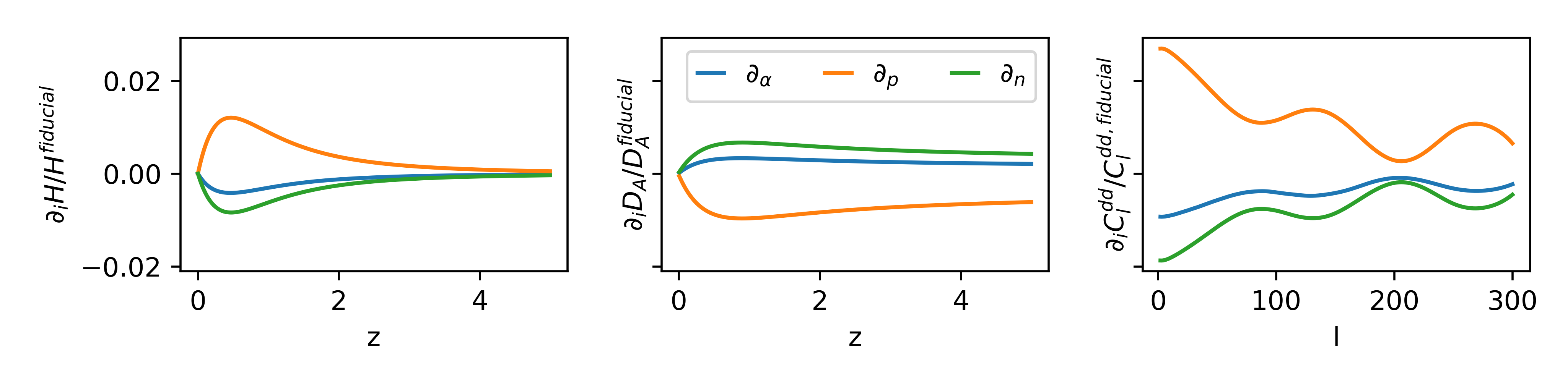
Figure 3: Numerical derivatives of the Hubble parameter, angular diameter distance and matter correlation. The computation was done for the case without maximum.

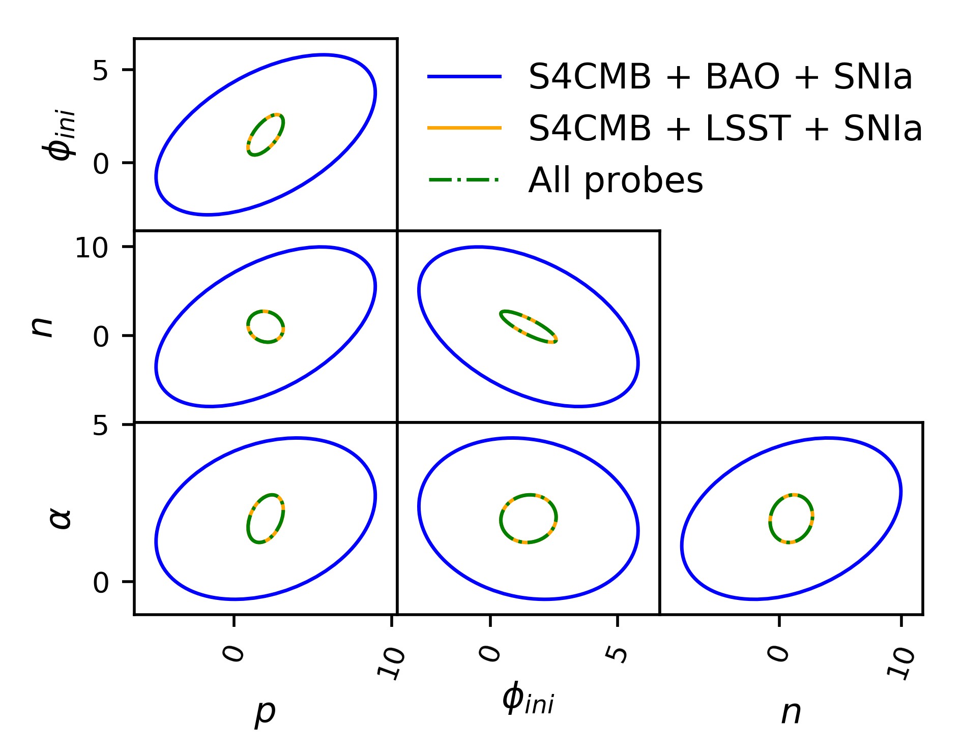
Figure 4: $2\sigma$-regions for the model parameters when the potential has no maximum. Note that the maximum constraints are already found for S4CMB + LSST + SNIa.

These constraints in the parameter space can also be seen in the CPL parametrization of dark energy ($w_{0}-w_{a}$) [67, 68]. In fact, one can see a similar improvement on the FoM (Table 8) of $w_{0}-w_{a}$ as in the model parameters (Table 7). The FoM for the CPL parameters has been defines as

$$\mbox{FoM}(w_{0},w_{a})=\frac{1}{\mbox{area}_{1\sigma}(w_{0},w_{a})},$$ (5.2)

which generalizes Eq. 5.1 for a non elliptical shape. It must be noted, however, that the main reason behind the large FoM is due to the fact that this model belongs to the thawing quintessence class, which is known to have little freedom in the $w_{0}-w_{a}$ plane [69]. Interestingly, it could be expected to detect a $2\sigma$ deviation from a cosmological constant ($w_{0}=-1$, $w_{a}=0$), provided that the fiducial model were the true one and one included LSST galaxy clustering observations (Fig. 5). This would not be the case if galaxy clustering were not taken into account. In fact, the weak constraints from the other cosmological probes would shift the $w_{0}-w_{a}$ $1\sigma$ region towards $w\sim-1$.

	FoM($w_{0},\,w_{a}$)
Experiments	w/o max.	$\psi_{ini}<\psi_{max}$	$\psi_{ini}>\psi_{max}$
S4CMB + BAO + SN Ia	$6\times 10^{2}$	$5\times 10^{1}$	$6\times 10^{2}$
S4CMB + gal.∗ + SNIa	$2\times 10^{3}$	$2\times 10^{2}$	$8\times 10^{3}$
All	$2\times 10^{3}$	$2\times 10^{2}$	$8\times 10^{3}$

Table 8: Figures of Merit (Eq. 5.1) for different combinations of future experiment on the $w_{0}$-$w_{a}$ parameters. BAO combines DESI and WFIRST predictions, SN Ia comes from constraints on $E(z)$ using WFIRST forecasts [38] and galaxy clustering (gal. cl) and shear (gal. sh) are those from LSST. The combination of galaxy clustering and shear has been written as gal.^∗.

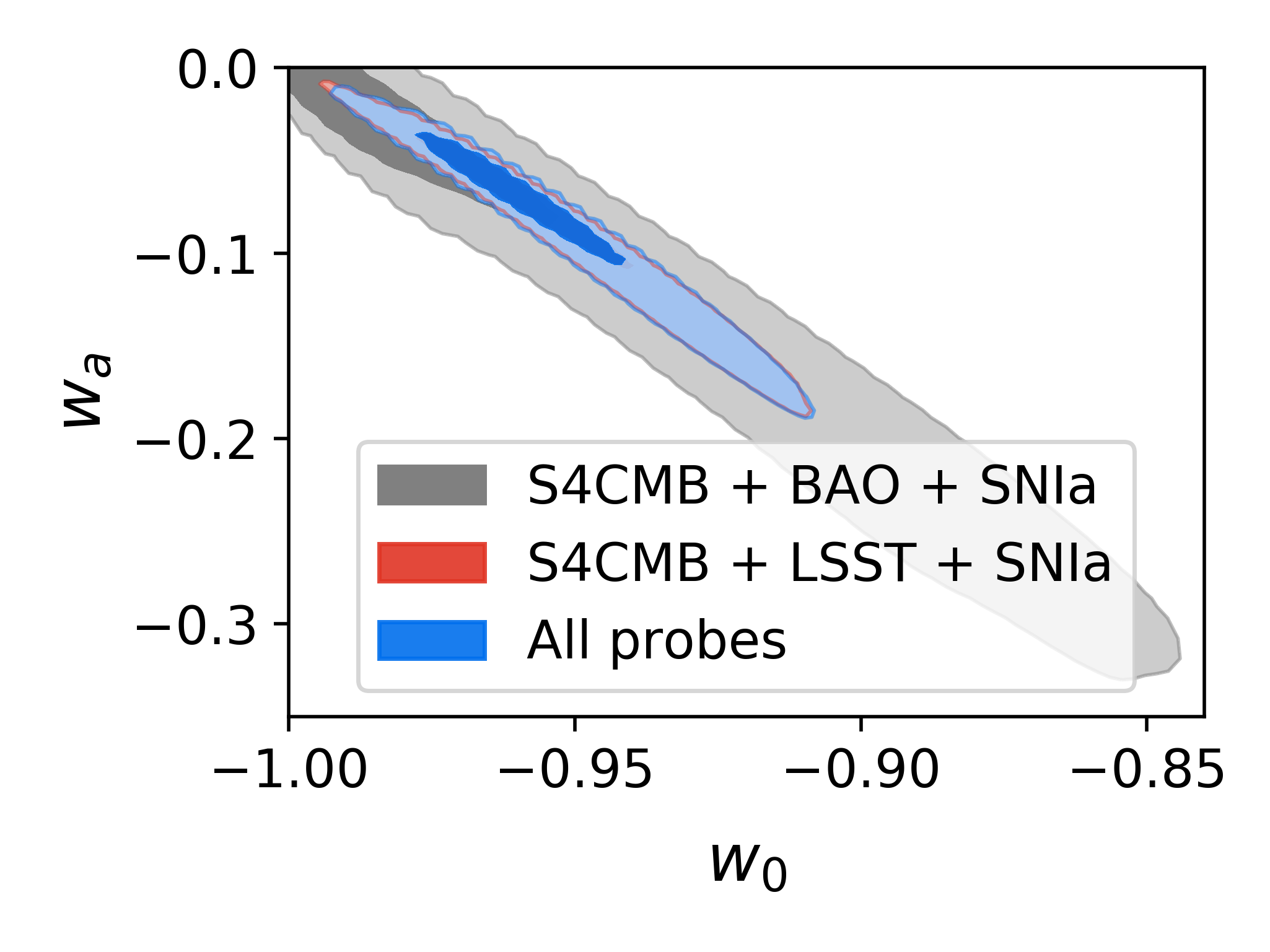
Figure 5: $2\sigma$-regions of the $w_{0}-w_{a}$ parameters parting from a fiducial model 1$\sigma$-off the $\Lambda$CDM regime and no maximum. Note that the maximum constraints are already found for S4CMB + LSST + SNIa.

The $w_{0}$-$w_{a}$ contours were obtained: first, we diagonalize the covariance matrix (i.e. $F^{-1}$). We then take samples of the uncorrelated Gaussian distribution and transform-back to the original basis. In doing so, we reject any model with $p<n$ (i.e. models with maximum) and with negative model parameters. Once selected, we used hi_class [61] to compute the corresponding $w_{0}$-$w_{a}$ parameters, with $w_{a}$ computed as $w_{a}=-dw/d\ln(a)|_{a=1}$). Finally, we used GetDist to produce contours of the corresponding samples.

5.2 Case with maximum: $p<n$

The fiducial model with maximum is given by $\{\alpha,\,p,\,n\}=\{2,\,2,\,3.5\}$. Given that the potential is not symmetric around the maximum, we will study the forecast potential of the next generation experiments with two fiducial models with initial value of the field so that it is at both sides of the maximum. It is located at $\psi_{max}=1.04$, and we will consider the cases with $\psi_{ini}=0.8,1.4$. The results are shown in Table 6, and the quantitative measurement of the constraining power of each probe is shown in Table 7. The found contours are shown in Fig. 6. As before, galaxy clustering will be the most constraining probe. In comparison, the case with $\psi_{ini}<\psi_{max}$ is better constrained, with S4-CMB experiments having a $\mbox{FoM}\sim 10^{-1}$ and, in combination with BAO and/or SNIa, $\mbox{FoM}\sim 1$. Using all probes, one can achieve a $\mbox{FoM}\sim 10^{2}$. However, for the case with $\psi_{ini}>\psi_{max}$, we only reach $\mbox{FoM}\sim 1$, when using all probes. The asymmetry around the maximum is such that at lower values, the potential slope is much more pronounced (see Fig. 2), making the model more sensitive to parameters changes. On the contrary, at values of the field greater than the maximum, the potential is softer and asymptotically flat, allowing for greater changes on the parameters that do not impact the final observables. The greater steepness of the potential is also the reason why the case with $\psi_{ini}<\psi_{max}$ is more constrained than the case without maximum (see Fig. 2), even though the dark energy equation of state of the fiducial model with maximum is closer to $w=-1$ (see Fig. 7), as a slightly lower $\psi_{ini}$ would make the field end up oscillating fast around $0$. It must be noted, however, that it is still $2\sigma$-off the exact $w=-1$.

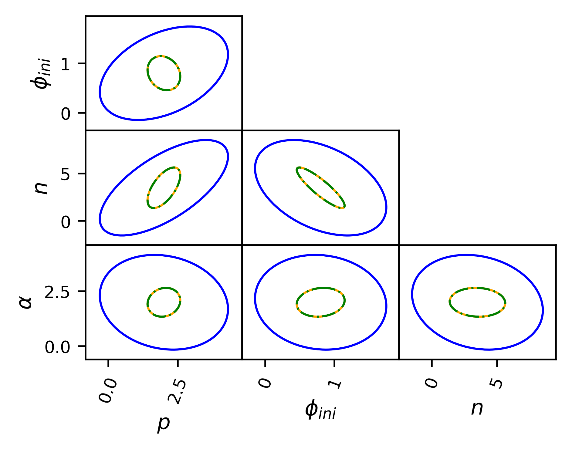
(a) $\psi_{ini}<\psi_{max}$

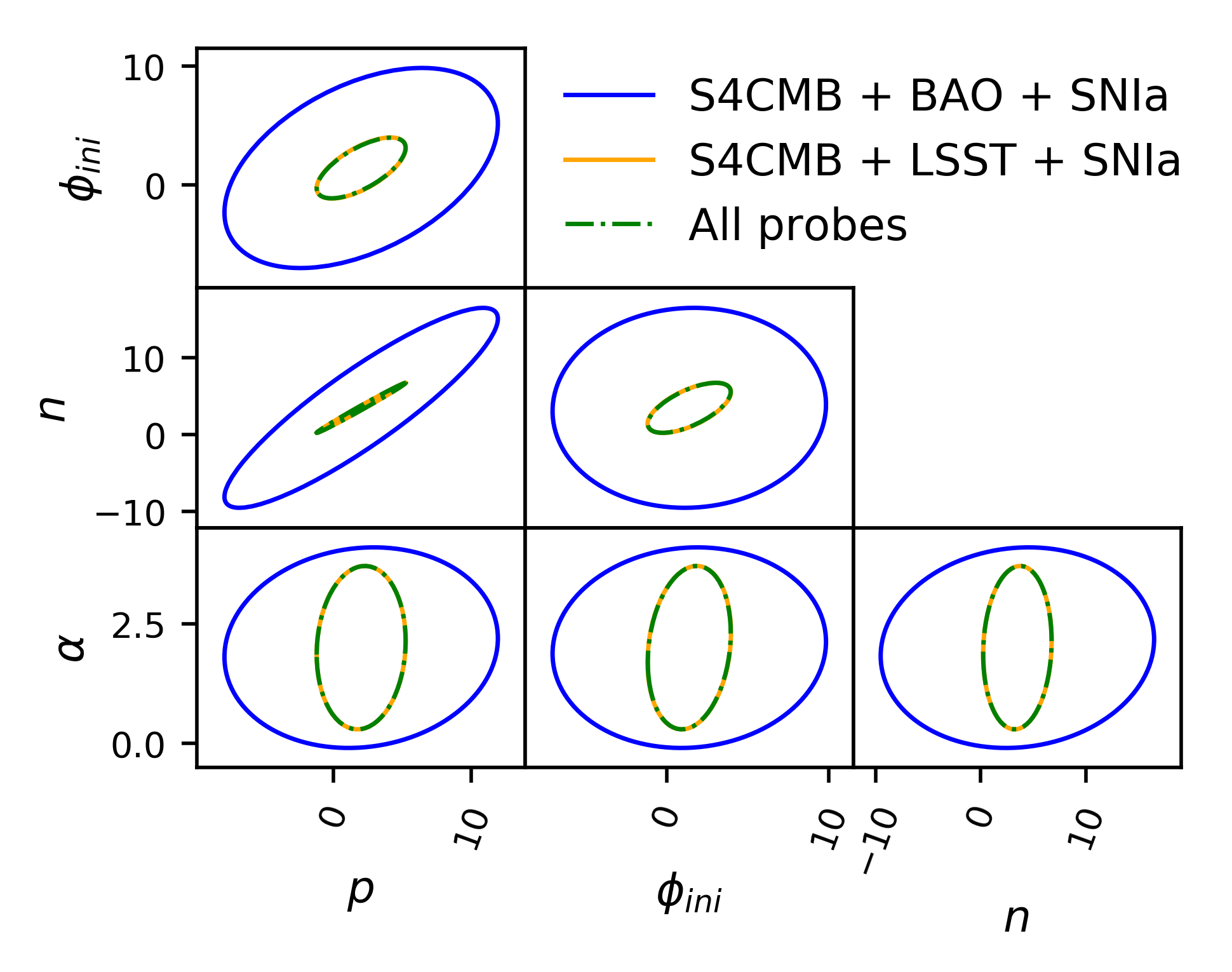
(b) $\psi_{ini}>\psi_{max}$

Figure 6: $2\sigma$-regions for the model parameters when the potential has a maximum. Note that the maximum constraints are already found for S4CMB + LSST + SNIa.

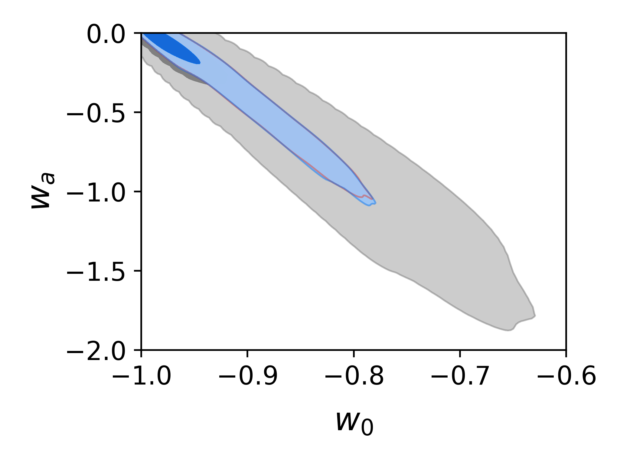
(a) $\psi_{ini}<\psi_{max}$

(b) $\psi_{ini}>\psi_{max}$

Figure 7: $2\sigma$-regions of the $w_{0}-w_{a}$ parameters parting from a fiducial model 1$\sigma$-off the $\Lambda$CDM regime. Note that the maximum constraints are already found for S4CMB + LSST + SNIa.

As in the previous section, the main restriction on the dark energy CPL parameters comes from being a thawing model. In particular, when $\psi_{ini}<\psi_{max}$, the field cannot start at much lower values than the fiducial $\psi_{ini}=0.8$, as the field would roll fast towards $\psi=0$. On the other hand, the constraints allow values of $\psi_{ini}$ that are closer to the maximum and the plateau, in the case with $\psi_{ini}>\psi_{max}$. As a consequence, the most likely parameter combinations that produce a correct late-time acceleration would be those with $w\sim-1$. Finally, the broader $2\sigma$-contours in the $\psi_{ini}<\psi_{max}$ case, despite of having a $\mbox{FoM}\sim 100$, over the model parameters, are a consequence of the larger range of accessible values of $V^{\prime}$ (see the potential shape in Fig. 2), which allows a richer variety of field evolutions. In addition, in all three cases, galaxy clustering is able to increase the $\mbox{FoM}(w_{0},\,w_{a})$ by almost an order of magnitude (see Table 8). The found contours have been plotted in Fig. 7

The FoM of the model and CPL parameters reflect the fact that the phenomenology of this model is mainly determined by its thawing nature and the initial position of the field, which determines what part of the potential is going to control the field evolution, and not all its parameters. In particular, the case with largest FoM on the model parameters is that with $\psi_{ini}<\psi_{max}$, while it is the one with lowest $\mbox{FoM}(w_{0},\,w_{a})$. Similarly, the configuration with $\psi_{ini}>\psi_{max}$ has the lowest FoM on the model parameters, but the greatest for the CPL parametrization. Finally, although the case without maximum has a $\mbox{FoM}(w_{0},\,w_{a})$ of same order as the former, its $\mbox{FoM}(\psi_{ini},\,\alpha,\,p,\,n)$ is an order of magnitude larger. Therefore, this shows the actual degrees of freedom, those that affect the phenomenology, are less than the number of free parameters; which we already know are degenerated. As a consequence, the $\mbox{FoM}(\psi_{ini},\,\alpha,\,p,\,n)$ is not a good quantity to inform us about how well constrained is the phenomenology of this model.

6 Comparison with previous results

Future observations will be able to greatly constrain the $\alpha$-attractor model, provided that the true dark energy model were different from a cosmological constant and $\alpha$ could not be arbitrarily large (i.e. $r\lesssim 0.01$). In this case, we have shown that a combination of S4CMB + LSST + SNIa, will greatily improve present results. In fact, they increase by almost an order of magnitude the FoM of both the parameter space and the $w_{0}-w_{a}$ parameters, when compared with S4CMB + BAO + SNIa.

A special comment is required for the results in the $w_{0}-w_{a}$ plane. In Figure 8 we have plotted the $w_{0}-w_{a}$ best $2\sigma$-contours, together with the results found in Ref. [19]. The available space for $w_{0}-w_{a}$ greatly depends on the fiducial cosmology used. For instance, if $\psi_{ini}<\psi_{max}$, the parameters are much less constrained. As we discussed in the previous section, this is caused by the fact that $V^{\prime}$ can have a broader range of values that will modify the acceleration of the field and, in turn, the evolution of the equation of state. In addition, it also shows that the $w_{0}-w_{a}$ CPL parametrization is not sufficient to describe the full evolution of the equation of state. In fact, viable and equivalent cosmologies can be obtained if the equation of state remains $w=-1$ for most of its evolution but grows fast close to the present or in case the equation of state diverged from $w=-1$ at early times but had a more monotonically growth along time. The other two cases are more restricted as the shape of the potential is softer and allows slower evolutions.

The case without maximum is $3\sigma$-off a cosmological constant solution; while the $\psi_{ini}<\psi_{max}$ is $2\sigma$-off. The case with $\psi_{ini}>\psi_{max}$ is concordant with $w=-1$ and is caused by the fact that a mild evolution of the field is allowed given the steepness at that side of the maximum (see Fig. 2) and the possibility of having $\psi_{ini}$ on the plateau by the loose constraints in the parameter space. It is important to note that the case with $\psi_{ini}>\psi_{max}$ is the only for which the constraints beat those imposed by current observations, which have a $\mbox{FoM}\sim 5\times 10^{3}$; although, given the mild constraints we have found in the parameter space, comparing the order of magnitude is a more conservative approach. This would be the case for the model without maximum. The reason why our result do not reduce the uncertainty in the $w_{0}-w_{a}$ CPL parameters is caused by the fact that the constraints that come from current observations (in blue in Fig. 8) are showing the preference of current data for a cosmological constant solution as this can be easily recovered thanks to the degeneracies of this model (see Section 2). In comparison with our current approach, the constraints from Ref. [19] were obtained by random sampling in the full parameter space, with non-informative priors. On the contrary, the constraints found in this work assume a fiducial model $1\sigma$-off a cosmological constant, and do not allow the parameters to change the case of study (e.g. $p<n$ when studying the case without maximum), limiting the possibility of going to the cosmological constant-like regime.

Figure 8: $w_{0}-w_{a}$ $2\sigma$ predicted regions when using all probes, compared with the result found in Ref. [19]. The case without maximum is $3\sigma$-off a cosmological constant; while the case with $\psi_{ini}<\psi_{max}$ is $2\sigma$-off. Forecast constraints are broader than those imposed by current observations [19] for various reasons. First, we are performing the forecasts around a specific fiducial cosmology, in contrast to the random sampling done in Ref. [19], where they explored all the parameter space without restriction. This shows that current observations favored $\Lambda$CDM, which is easily recovered in this model (Section 2). In addition, a fiducial model $1\sigma$-off a cosmological constant is being used for the forecast analysis. Finally, for the particular case with $\psi_{ini}<\psi_{max}$, the $w_{0}-w_{a}$ parameters are not accurate descriptors of the equation of state, as equivalent cosmological evolutions can be obtained if $w$ slowly varies since early times than in the case it remains close to $w=-1$, but close to the present greatly diverges. Nevertheless, the resulting FoM for the $\psi_{ini}>\psi_{max}$ case ($8\times 10^{3}$) is larger than that with current data ($\sim 5\times 10^{3}$) and for the case without maximum it is still of the same order of magnitude ($2\times 10^{3}$).

7 Conclusions

In this work, we analyze the $\alpha$-attractor dark energy model [9] in the context of near-future cosmological experiments. This model was already studied with current observations in Ref. [19] and seen to be unbounded, as a consequence of the existing parameter degeneracies; in particular, between $\alpha-\psi_{ini}$ and $p-n$, the potential exponents.

Next-generation experiments will be able to measure the cosmological observables with percent-level precision. For the specific case with a maximum ($p<n$) and $\psi_{ini}<\psi_{max}$, we have found an important improvement on the constraints with respect to current bounds. However, this improvement does not translate into a significant reduction of uncertainties in the equation of state parameters under the CPL parametrization. This is due to the restrictions of the model in this space of parameters. On the other hand, the case with $\psi_{ini}>\psi_{max}$ is almost insensitive to the additional constraining power of next-generation datasets. Interestingly, in case that true underlying model were that without maximum, and sufficiently distinct from $\Lambda$CDM, one could detect a $3\sigma$ deviation from a pure cosmological constant; and a $2\sigma$ deviation if $\psi_{ini}<\psi_{max}$.

The use of CMB-S4 and other future CMB experiments to place constraints on the tensor-to-scalar ratio, $r$, and the spectral index, $n_{s}$, to constrain $\alpha$ (see Eq. 2.5), is unlikely to provide any significant improvement over the results shown here, since those constraints will still allow for too much freedom, leaving the results shown in Ref. [19] almost untouched.

Finally, the use of tomographic galaxy clustering would be particularly important in order to achieve this. From the analysis of individual probes (see the Figures of Merit in Table 7), we have shown that galaxy clustering will be the probe with the most constraining capability, since the galaxy power spectrum is the most sensitive observable (Fig. 3) to changes in the $\alpha$-attractor parameters. We find this statement to be true across the different fiducial models studied. In particular, the combination S4CMB + LSST + SNIa will improve the FoM of both the parameter space and $w_{0}-w_{a}$ by almost an order of magnitude with respect to the case with S4CMB + BAO + SNIa.

Next-generation experiments will lead us to an unprecedented level of precision in cosmology, allowing us to test our knowledge about the Universe, its origin and dynamical evolution. In this work we have shown how these observations, in particular a combination of CMB, galaxy and SNIa measurements will be able to set constraints on the dark energy $\alpha$-attractor model and, as a consequence, we would expect that, in general, future surveys will be able to probe whether the late accelerated expansion of the Universe is connected with the one the Universe started with – inflation.

References

- [1] A. Linde, Inflationary Cosmology after Planck 2013, in Proceedings, 100th Les Houches Summer School: Post-Planck Cosmology: Les Houches, France, July 8 - August 2, 2013, pp. 231–316, 2015. arXiv:1402.0526.
- [2] Planck Collaboration, Y. Akrami et al., Planck 2018 results. X. Constraints on inflation, arXiv:1807.06211.
- [3] Supernova Search Team Collaboration, A. G. Riess et al., Observational evidence from supernovae for an accelerating universe and a cosmological constant, Astron. J. 116 (1998) 1009–1038, [astro-ph/9805201].
- [4] Supernova Cosmology Project Collaboration, S. Perlmutter et al., Measurements of Omega and Lambda from 42 high redshift supernovae, Astrophys. J. 517 (1999) 565–586, [astro-ph/9812133].
- [5] DES Collaboration, T. M. C. Abbott et al., First Cosmology Results using Type Ia Supernovae from the Dark Energy Survey: Constraints on Cosmological Parameters, Astrophys. J. 872 (2019), no. 2 L30, [arXiv:1811.02374].
- [6] D. Spergel et al., Wide-Field InfraRed Survey Telescope-Astrophysics Focused Telescope Assets WFIRST-AFTA Final Report, arXiv:1305.5422.
- [7] Planck Collaboration, N. Aghanim et al., Planck 2018 results. VI. Cosmological parameters, arXiv:1807.06209.
- [8] BOSS Collaboration, S. Alam et al., The clustering of galaxies in the completed SDSS-III Baryon Oscillation Spectroscopic Survey: cosmological analysis of the DR12 galaxy sample, Mon. Not. Roy. Astron. Soc. 470 (2017), no. 3 2617–2652, [arXiv:1607.03155].
- [9] E. V. Linder, Dark Energy from -Attractors, Phys. Rev. D91 (2015), no. 12 123012, [arXiv:1505.00815].
- [10] K. Dimopoulos and C. Owen, Quintessential Inflation with -attractors, JCAP 1706 (2017), no. 06 027, [arXiv:1703.00305].
- [11] K. Dimopoulos and C. Owen, Instant Preheating in Quintessential Inflation with -Attractors, arXiv:1712.01760.
- [12] Y. Akrami, R. Kallosh, A. Linde, and V. Vardanyan, Dark energy, -attractors, and large-scale structure surveys, arXiv:1712.09693.
- [13] S. Casas, M. Pauly, and J. Rubio, Higgs-dilaton cosmology: An inflation–dark-energy connection and forecasts for future galaxy surveys, Phys. Rev. D97 (2018), no. 4 043520, [arXiv:1712.04956].
- [14] K. Dimopoulos and T. Markkanen, Dark energy as a remnant of inflation and electroweak symmetry breaking, JHEP 01 (2019) 029, [arXiv:1807.04359].
- [15] S. Casas, G. K. Karananas, M. Pauly, and J. Rubio, Scale-invariant alternatives to general relativity. III. The inflation-dark energy connection, Phys. Rev. D99 (2019), no. 6 063512, [arXiv:1811.05984].
- [16] J. E. Camargo-Molina, T. Markkanen, and P. Scott, Dark energy without fine tuning, arXiv:1905.00045.
- [17] M. Shahalam, R. Myrzakulov, S. Myrzakul, and A. Wang, Observational constraints on the generalized attractor model, Int. J. Mod. Phys. D27 (2018) 1850058, [arXiv:1611.06315].
- [18] S. Bag, S. S. Mishra, and V. Sahni, New tracker models of dark energy, arXiv:1709.09193.
- [19] C. García-García, E. V. Linder, P. Ruíz-Lapuente, and M. Zumalacárregui, Dark energy from -attractors: phenomenology and observational constraints, JCAP 1808 (2018), no. 08 022, [arXiv:1803.00661].
- [20] F. X. L. Cedeño, A. Montiel, J. C. Hidalgo, and G. Germán, Bayesian evidence for -attractor dark energy models, arXiv:1905.00834.
- [21] A. A. Starobinsky, A New Type of Isotropic Cosmological Models Without Singularity, Phys. Lett. 91B (1980) 99–102.
- [22] S. D. Odintsov and V. K. Oikonomou, Inflationary -attractors from gravity, Phys. Rev. D94 (2016), no. 12 124026, [arXiv:1612.01126].
- [23] T. Miranda, J. C. Fabris, and O. F. Piattella, Reconstructing a theory from the -Attractors, JCAP 1709 (2017), no. 09 041, [arXiv:1707.06457].
- [24] S. S. Mishra, V. Sahni, and Y. Shtanov, Sourcing Dark Matter and Dark Energy from -attractors, JCAP 1706 (2017), no. 06 045, [arXiv:1703.03295].
- [25] WMAP Collaboration, G. Hinshaw et al., Nine-Year Wilkinson Microwave Anisotropy Probe (WMAP) Observations: Cosmological Parameter Results, Astrophys. J. Suppl. 208 (2013) 19, [arXiv:1212.5226].
- [26] M. Galante, R. Kallosh, A. Linde, and D. Roest, Unity of Cosmological Inflation Attractors, Phys. Rev. Lett. 114 (2015), no. 14 141302, [arXiv:1412.3797].
- [27] R. Kallosh and A. Linde, Universality Class in Conformal Inflation, JCAP 1307 (2013) 002, [arXiv:1306.5220].
- [28] DESI Collaboration, A. Aghamousa et al., The DESI Experiment Part I: Science,Targeting, and Survey Design, arXiv:1611.00036.
- [29] A. Font-Ribera, P. McDonald, N. Mostek, B. A. Reid, H.-J. Seo, and A. Slosar, DESI and other dark energy experiments in the era of neutrino mass measurements, JCAP 1405 (2014) 023, [arXiv:1308.4164].
- [30] K. N. Abazajian et al., Inflation Physics from the Cosmic Microwave Background and Large Scale Structure, Astropart. Phys. 63 (2015) 55–65, [arXiv:1309.5381].
- [31] LSST Science, LSST Project Collaboration, P. A. Abell et al., LSST Science Book, Version 2.0, arXiv:0912.0201.
- [32] U. Seljak, Extracting primordial non-gaussianity without cosmic variance, Phys. Rev. Lett. 102 (2009) 021302, [arXiv:0807.1770].
- [33] D. Alonso and P. G. Ferreira, Constraining ultralarge-scale cosmology with multiple tracers in optical and radio surveys, Phys. Rev. D92 (2015), no. 6 063525, [arXiv:1507.03550].
- [34] B. Whitt, Fourth Order Gravity as General Relativity Plus Matter, Phys. Lett. 145B (1984) 176–178.
- [35] K.-i. Maeda, Inflation as a Transient Attractor in Cosmology, Phys. Rev. D37 (1988) 858.
- [36] J. D. Barrow, The Premature Recollapse Problem in Closed Inflationary Universes, Nucl. Phys. B296 (1988) 697–709.
- [37] Planck Collaboration, P. A. R. Ade et al., Planck 2015 results. XIV. Dark energy and modified gravity, Astron. Astrophys. 594 (2016) A14, [arXiv:1502.01590].
- [38] A. G. Riess et al., Type Ia Supernova Distances at from the Hubble Space Telescope Multi-Cycle Treasury Programs: The Early Expansion Rate, arXiv:1710.00844.
- [39] E. Calabrese et al., Precision Epoch of Reionization studies with next-generation CMB experiments, JCAP 1408 (2014) 010, [arXiv:1406.4794].
- [40] SPT-3G Collaboration, B. A. Benson et al., SPT-3G: A Next-Generation Cosmic Microwave Background Polarization Experiment on the South Pole Telescope, Proc. SPIE Int. Soc. Opt. Eng. 9153 (2014) 91531P, [arXiv:1407.2973].
- [41] BICEP2, Keck Array Collaboration, P. A. R. Ade et al., Improved Constraints on Cosmology and Foregrounds from BICEP2 and Keck Array Cosmic Microwave Background Data with Inclusion of 95 GHz Band, Phys. Rev. Lett. 116 (2016) 031302, [arXiv:1510.09217].
- [42] POLARBEAR Collaboration, A. Suzuki et al., The POLARBEAR-2 and the Simons Array Experiment, J. Low. Temp. Phys. 184 (2016), no. 3-4 805–810, [arXiv:1512.07299].
- [43] Planck Collaboration, P. A. R. Ade et al., Planck 2013 results. XVI. Cosmological parameters, Astron. Astrophys. 571 (2014) A16, [arXiv:1303.5076].
- [44] A. Lewis and A. Challinor, Weak gravitational lensing of the CMB, Phys. Rept. 429 (2006) 1–65, [astro-ph/0601594].
- [45] W. Hu and T. Okamoto, Mass reconstruction with cmb polarization, Astrophys. J. 574 (2002) 566–574, [astro-ph/0111606].
- [46] D. Alonso, P. Bull, P. G. Ferreira, R. Maartens, and M. Santos, Ultra large-scale cosmology in next-generation experiments with single tracers, Astrophys. J. 814 (2015), no. 2 145, [arXiv:1505.07596].
- [47] SDSS Collaboration, I. Strateva et al., Color separation of galaxy types in the Sloan Digital Sky Survey imaging data, Astron. J. 122 (2001) 1861–1874, [astro-ph/0107201].
- [48] H. J. Mo and S. D. M. White, An analytic model for the spatial clustering of dark matter haloes, Mon. Not. Roy. Astron. Soc. 282 (Sep, 1996) 347–361, [astro-ph/9512127].
- [49] D. H. Weinberg, R. Dave, N. Katz, and L. Hernquist, Galaxy clustering and galaxy bias in a lambda-CDM universe, Astrophys. J. 601 (2004) 1–21, [astro-ph/0212356].
- [50] A. L. Coil et al., The DEEP2 Galaxy Redshift Survey: Color and luminosity dependence of galaxy clustering at z similar to 1, Astrophys. J. 672 (2008) 153–176, [arXiv:0708.0004].
- [51] I. Mohammed, U. Seljak, and Z. Vlah, Perturbative approach to covariance matrix of the matter power spectrum, Mon. Not. Roy. Astron. Soc. 466 (2017), no. 1 780–797, [arXiv:1607.00043].
- [52] C. S. Lorenz, D. Alonso, and P. G. Ferreira, Impact of relativistic effects on cosmological parameter estimation, Phys. Rev. D97 (2018), no. 2 023537, [arXiv:1710.02477].
- [53] D. H. Rudd, A. R. Zentner, and A. V. Kravtsov, Effects of Baryons and Dissipation on the Matter Power Spectrum, Astrophys. J. 672 (2008) 19–32, [astro-ph/0703741].
- [54] M. P. van Daalen, J. Schaye, C. M. Booth, and C. D. Vecchia, The effects of galaxy formation on the matter power spectrum: A challenge for precision cosmology, Mon. Not. Roy. Astron. Soc. 415 (2011) 3649–3665, [arXiv:1104.1174].
- [55] M. P. van Daalen, J. Schaye, I. G. McCarthy, C. M. Booth, and C. Dalla Vecchia, The impact of baryonic processes on the two-point correlation functions of galaxies, subhaloes and matter, Mon. Not. Roy. Astron. Soc. 440 (2014), no. 4 2997–3010, [arXiv:1310.7571].
- [56] W. A. Hellwing, M. Schaller, C. S. Frenk, T. Theuns, J. Schaye, R. G. Bower, and R. A. Crain, The effect of baryons on redshift space distortions and cosmic density and velocity fields in the EAGLE simulation, Mon. Not. Roy. Astron. Soc. 461 (2016), no. 1 L11–L15, [arXiv:1603.03328].
- [57] J. Harnois-Déraps, L. van Waerbeke, M. Viola, and C. Heymans, Baryons, Neutrinos, Feedback and Weak Gravitational Lensing, Mon. Not. Roy. Astron. Soc. 450 (2015), no. 2 1212–1223, [arXiv:1407.4301].
- [58] N. E. Chisari, M. L. A. Richardson, J. Devriendt, Y. Dubois, A. Schneider, M. C. Brun, Amandine Le, R. S. Beckmann, S. Peirani, A. Slyz, and C. Pichon, The impact of baryons on the matter power spectrum from the Horizon-AGN cosmological hydrodynamical simulation, arXiv:1801.08559.
- [59] H.-J. Huang, T. Eifler, R. Mandelbaum, and S. Dodelson, Modeling baryonic physics in future weak lensing surveys, arXiv:1809.01146.
- [60] R. Hounsell et al., Simulations of the WFIRST Supernova Survey and Forecasts of Cosmological Constraints, Astrophys. J. 867 (2018), no. 1 23, [arXiv:1702.01747].
- [61] M. Zumalacárregui, E. Bellini, I. Sawicki, J. Lesgourgues, and P. G. Ferreira, hi_class: Horndeski in the Cosmic Linear Anisotropy Solving System, JCAP 1708 (2017), no. 08 019, [arXiv:1605.06102].
- [62] D. Blas, J. Lesgourgues, and T. Tram, The Cosmic Linear Anisotropy Solving System (CLASS) II: Approximation schemes, JCAP 1107 (2011) 034, [arXiv:1104.2933].
- [63] G. W. Horndeski, Second-order scalar-tensor field equations in a four-dimensional space, Int. J. Theor. Phys. 10 (1974) 363–384.
- [64] I. Sawicki and E. Bellini, Limits of quasistatic approximation in modified-gravity cosmologies, Phys. Rev. D92 (2015), no. 8 084061, [arXiv:1503.06831].
- [65] D. N. Limber, The Analysis of Counts of the Extragalactic Nebulae in Terms of a Fluctuating Density Field., Astrophys. J. 117 (Jan., 1953) 134.
- [66] A. Albrecht et al., Report of the Dark Energy Task Force, astro-ph/0609591.
- [67] M. Chevallier and D. Polarski, Accelerating universes with scaling dark matter, Int. J. Mod. Phys. D10 (2001) 213–224, [gr-qc/0009008].
- [68] E. V. Linder, Exploring the expansion history of the universe, Phys. Rev. Lett. 90 (2003) 091301, [astro-ph/0208512].
- [69] E. V. Linder, Quintessence’s last stand?, Phys. Rev. D91 (2015) 063006, [arXiv:1501.01634].