Probing neutrino transition magnetic moments
with coherent elastic neutrino-nucleus scattering

Abstract

We explore the potential of current and next generation of coherent elastic neutrino-nucleus scattering (CE$\nu$NS) experiments in probing neutrino electromagnetic interactions. On the basis of a thorough statistical analysis, we determine the sensitivities on each component of the Majorana neutrino transition magnetic moment (TMM), $\left|\Lambda_{i}\right|$, that follow from low-energy neutrino-nucleus experiments. We derive the sensitivity to neutrino TMM from the first CE$\nu$NS measurement by the COHERENT experiment, at the Spallation Neutron Source. We also present results for the next phases of COHERENT using HPGe, LAr and NaI[Tl] detectors and for reactor neutrino experiments such as CONUS, CONNIE, MINER, TEXONO and RED100. The role of the CP violating phases in each case is also briefly discussed. We conclude that future CE$\nu$NS experiments with low-threshold capabilities can improve current TMM limits obtained from Borexino data.

1 Introduction

One of the major recent milestones in particle physics has been the discovery of neutrino oscillations [1, 2, 3, 4, 5]. It implies that neutrinos are massive and, hence, new physics must exist in order to provide neutrino masses and mixings [6, 7]. Massive neutrinos are expected to have non-trivial electromagnetic properties such as magnetic moments and charge radius [8, 9, 10, 11, 12, 13, 14, 15]. Here we focus on the former. Although the expected magnitude of magnetic moments is typically small, it is rather model-dependent and constitutes a precious probe of physics beyond the Standard Model (SM).

The recent observation of neutral-current coherent elastic neutrino-nucleus scattering (CE$\nu$NS) by the COHERENT experiment [16, 17] has given access to a wide range of new physics opportunities. This has prompted numerous proposals to search for physics beyond the SM [18, 19, 20, 21] with a special focus on non-standard neutrino interactions with matter [22, 23, 24, 25, 26, 27, 28], sterile neutrinos [29, 30, 31], novel mediators [32, 33, 34, 35] and dark matter [36, 37]. Moreover, CE$\nu$NS has been also suggested as a prominent tool towards exploring important nuclear structure parameters [38, 39], as well as implications for physics within [40, 41] and beyond the Standard Model  [42, 43, 44]. Very recently, it has been emphasized the need for taking into account also the incoherent channel of neutrino-nucleus scattering at momentum transfers ($q$) beyond the coherency frontier, e.g. $qR_{A}\gg 1$ [45] ($R_{A}$ is the nuclear radius), which are particularly relevant for neutrino floor studies at direct detection dark matter experiments [46, 47, 48].

Here, we examine the potential of the upcoming experiments to probe neutrino magnetic moments in their most general realization, namely transition magnetic moments (TMMs) of Majorana neutrinos [8]. We explore the discovery potential of these experiments to sub-leading effects associated to neutrino TMMs through the measurement of the CE$\nu$NS event rate. Then, upon the work presented in [49, 50, 51], we build up a dedicated study on low-energy neutrino-nucleus processes, in the light of current and upcoming CE$\nu$NS experiments. In particular, we examine the potential of planned reactor neutrino experiments CONUS [52], CONNIE [53], MINER [54], TEXONO [55] and RED100 [56], and several variants of the recent COHERENT experiment [16, 57, 17] at the Spallation Neutron Source (SNS) in probing neutrino TMMs. We quantify the sensitivities expected for different target materials, detector sizes, thresholds, efficiencies, exposure times and baseline choices. Our results are determined on the basis of a dedicated $\chi^{2}$ analysis that takes into account as well the quenching effects, relevant for high purity sub-keV threshold detectors. We conclude that neutral-current coherent elastic neutrino-nucleus scattering studies at these facilities offer the capability of probing electromagnetic neutrino properties such as neutrino TMMs with improved sensitivities, hence providing a sensitive way to test for new physics in the neutrino sector. Beyond the analysis of CE$\nu$NS experiments, in this work we update the discussion given in Refs. [49, 50, 51] concerning the sensitivity of $\nu-e$ scattering to the effective neutrino magnetic moment using the solar neutrino data from the Borexino collaboration [58]. We also briefly comment on alternatives to probe the effective neutrino magnetic moments using other neutrino sources that contribute to the neutrino floor in dark matter direct detection experiments, such as solar and geoneutrinos, as well as atmospheric and diffuse supernova neutrinos.

The paper has been organized as follows. In Sect. 2, we introduce the main theoretical background and derive the expressions for the effective neutrino magnetic moments corresponding to the various neutrino sources under study. In Sect. 3, we discuss the main features associated with the relevant electromagnetic CE$\nu$NS processes, while in Sect. 4 we define the experimental configurations and setups for the different CE$\nu$NS experiments of interest. Our results are presented in Sect. 5. A brief discussion, including updated constraints from the recent Borexino data, and comments on other neutrino sources that might be relevant to the neutrino floor in dark matter direct detection experiments are given in Sect. 6. Finally, the main conclusions are given in Sect. 7.

2 Theoretical framework

The effective Hamiltonian that accounts for the spin component of the Majorana neutrino electromagnetic vertex is expressed in terms of the electromagnetic field tensor $F_{\alpha\beta}$, as [8, 7]

$$H_{\text{EM}}^{\mathrm{M}}=-\frac{1}{4}\nu_{L}^{\mathsf{T}}C^{-1}\lambda\sigma^{\alpha\beta}\nu_{L}F_{\alpha\beta}+\mathrm{h.c.}\,,$$ (1)

with $\lambda=\mu-i\epsilon$ being an antisymmetric complex matrix ($\lambda_{\alpha\beta}=-\lambda_{\beta\alpha}$) and, hence, $\mu^{\mathsf{T}}=-\mu$ and $\epsilon^{\mathsf{T}}=-\epsilon$ are two imaginary matrices. Therefore, three complex or six real parameters are required to describe this object. The corresponding Hamiltonian relevant to the Dirac neutrino case reads

$$H_{\text{EM}}^{\mathrm{D}}=\frac{1}{2}\bar{\nu}_{R}\lambda\sigma^{\alpha\beta}\nu_{L}F_{\alpha\beta}+\mathrm{h.c.}\,,$$ (2)

where $\lambda=\mu-i\epsilon$ is a complex matrix, subject to the hermiticity constraints $\mu=\mu^{\dagger}$ and $\epsilon=\epsilon^{\dagger}$. Comparing Eqs. (1) and (2), it becomes evident that neutrino electromagnetic properties constitute a prime vehicle to distinguish between the Dirac and Majorana neutrino nature. In contrast to the Dirac case, vanishing diagonal moments are implied for Majorana neutrinos, $\mu^{\mathrm{M}}_{ii}=\epsilon^{\mathrm{M}}_{ii}=0$. In the simplest $\mathrm{SU(2)_{L}\otimes U(1)_{Y}}$ model, the Majorana magnetic and electric transition moments (with $i\neq j$) take the form [9]

$$\mu_{ij}^{\mathrm{M}}=-\frac{3ieG_{F}}{16\pi^{2}\sqrt{2}}(m_{\nu i}+m_{\nu j})\sum_{\alpha=e,\mu,\tau}\Im m\left[U_{\alpha i}^{\ast}U_{\alpha j}\left(\frac{m_{l\alpha}}{M_{W}}\right)^{2}\right]\,,$$ (3)

$$\epsilon_{ij}^{\mathrm{M}}=\frac{3ieG_{F}}{16\pi^{2}\sqrt{2}}(m_{\nu i}-m_{\nu j})\sum_{\alpha=e,\mu,\tau}\Re e\left[U_{\alpha i}^{\ast}U_{\alpha j}\left(\frac{m_{l\alpha}}{M_{W}}\right)^{2}\right]\,,$$ (4)

where $G_{F}$ is the Fermi coupling constant, $m_{\nu_{i}}$ is the mass of the neutrino mass eigenstate $\nu_{i}$, $U_{\alpha i}$ denote the elements of the neutrino mixing matrix, while $m_{l\alpha}$ and $M_{W}$ correspond to the charged lepton and W boson masses, respectively.

In this work, we will focus on the study of the Majorana transition magnetic moment $\mu_{ij}^{\mathrm{M}}$. For simplicity, we will drop the superscript M referring to Majorana neutrinos from now on. The effective neutrino magnetic moment, observable in a given experiment, can be expressed in terms of the neutrino magnetic moment matrix and the amplitudes of positive and negative helicity states, denoted by the $3-$vectors $\mathfrak{a}_{+}$ and $\mathfrak{a}_{-}$, respectively. In the flavor basis one finds [59]

$$\left(\mu_{\nu}^{F}\right)^{2}=\mathfrak{a}_{-}^{\dagger}\lambda^{\dagger}\lambda\mathfrak{a}_{-}+\mathfrak{a}_{+}^{\dagger}\lambda\lambda^{\dagger}\mathfrak{a}_{+}\,,$$ (5)

with the magnetic moment matrix $\lambda$ ($\tilde{\lambda}$) in the flavor (mass) basis defined as

$$\lambda=\left(\begin{array}[]{ccc}0&\Lambda_{\tau}&-\Lambda_{\mu}\\ -\Lambda_{\tau}&0&\Lambda_{e}\\ \Lambda_{\mu}&-\Lambda_{e}&0\end{array}\right),\qquad\tilde{\lambda}=\left(\begin{array}[]{ccc}0&\Lambda_{3}&-\Lambda_{2}\\ -\Lambda_{3}&0&\Lambda_{1}\\ \Lambda_{2}&-\Lambda_{1}&0\end{array}\right)\,.$$ (6)

In this context, the definition $\lambda_{\alpha\beta}=\varepsilon_{\alpha\beta\gamma}\Lambda_{\gamma}$ has been introduced, and the neutrino TMMs are represented by the complex parameters [50]

$$\Lambda_{\alpha}=|\Lambda_{\alpha}|e^{i\zeta_{\alpha}},\qquad\Lambda_{i}=|\Lambda_{i}|e^{i\zeta_{i}}\,.$$ (7)

The effective neutrino magnetic moment in the flavor basis, shown in Eq. (5), can be translated into the mass basis through a rotation, by using the leptonic mixing matrix. Then, by introducing the transformations

$$\tilde{\mathfrak{a}}_{-}=U^{\dagger}\mathfrak{a}_{-},\qquad\tilde{\mathfrak{a}}_{+}=U^{\mathsf{T}}\mathfrak{a}_{+},\qquad\tilde{\lambda}=U^{\mathsf{T}}\lambda U\,,$$ (8)

the effective neutrino magnetic moment in the mass basis takes the form [51]

$$\left(\mu_{\nu}^{M}\right)^{2}=\tilde{\mathfrak{a}}_{-}^{\dagger}\tilde{\lambda}^{\dagger}\tilde{\lambda}\tilde{\mathfrak{a}}_{-}+\tilde{\mathfrak{a}}_{+}^{\dagger}\tilde{\lambda}\tilde{\lambda}^{\dagger}\tilde{\mathfrak{a}}_{+}\,.$$ (9)

2.1 Effective neutrino magnetic moment at reactor CE$\nu$NS experiments

For CE$\nu$NS studies at reactor neutrino experiments, the only non-zero parameter entering Eq. (5) or Eq. (9) is $\mathfrak{a}_{+}^{1}$, corresponding to the initial $\bar{\nu}_{e}$ flux. Then, in the flavor basis, the effective Majorana TMM strength parameter relevant to reactor CE$\nu$NS experiments such as CONUS, CONNIE, MINER, TEXONO and RED100, can be cast in the form [51]

$$\left(\mu_{\bar{\nu}_{e},\,\text{reactor}}^{F}\right)^{2}=|\Lambda_{\mu}|^{2}+|\Lambda_{\tau}|^{2}\,,$$ (10)

where $|\Lambda_{\mu}|$ and $|\Lambda_{\tau}|$ denote the elements of the neutrino transition magnetic moment matrix $\lambda$ describing the corresponding conversions from the electron antineutrino to the muon and tau neutrino states, respectively. The above expression, in the mass basis becomes  [49]

$$\left(\mu_{\bar{\nu}_{e},\,\text{reactor}}^{M}\right)^{2}= |\mathbf{\Lambda}|^{2}-c_{12}^{2}c_{13}^{2}|\Lambda_{1}|^{2}-s_{12}^{2}c_{13}^{2}|\Lambda_{2}|^{2}-s_{13}^{2}|\Lambda_{3}|^{2}$$ (11)

$$-c_{13}^{2}\sin 2\theta_{12}|\Lambda_{1}||\Lambda_{2}|\cos(\zeta_{1}-\zeta_{2})$$

$$-c_{12}\sin 2\theta_{13}|\Lambda_{1}||\Lambda_{3}|\cos(\delta_{\text{CP}}+\zeta_{1}-\zeta_{3})$$

$$-s_{12}\sin 2\theta_{13}|\Lambda_{2}||\Lambda_{3}|\cos(\delta_{\text{CP}}+\zeta_{2}-\zeta_{3})\,,$$

where $|\Lambda_{i}|$ and $\zeta_{i}$ are the moduli and phases characterizing the neutrino TMM matrix in the mass basis, see Eq. (7). We have also defined $|\mathbf{\Lambda}|^{2}=|\Lambda_{1}|^{2}+|\Lambda_{2}|^{2}+|\Lambda_{3}|^{2}$ and used the standard abbreviations $c_{ij}=\cos\theta_{ij}$, $s_{ij}=\sin\theta_{ij}$ for the trigonometric functions of the neutrino mixing angles. As usual, $\delta_{\text{CP}}$ refers to the Dirac CP phase of the leptonic mixing matrix.

The expression above can be further simplified by defining a new set of phases $\xi_{i}$ as the differences of the TMM phases: $\xi_{1}=\zeta_{3}-\zeta_{2}$, $\xi_{2}=\zeta_{3}-\zeta_{1}$ and $\xi_{3}=\zeta_{1}-\zeta_{2}$. Note that $\xi_{2}=\xi_{1}-\xi_{3}$ and, therefore, only two $\xi_{i}$ phases are independent. In the following, we will express the effective neutrino magnetic moments as a function of the $\delta_{\text{CP}}$ and $\xi_{i}$ phases. With this notation, the effective neutrino magnetic moment in Eq. (11) will be expressed as

$$\left(\mu_{\bar{\nu}_{e},\,\text{reactor}}^{M}\right)^{2}= |\mathbf{\Lambda}|^{2}-c_{12}^{2}c_{13}^{2}|\Lambda_{1}|^{2}-s_{12}^{2}c_{13}^{2}|\Lambda_{2}|^{2}-s_{13}^{2}|\Lambda_{3}|^{2}$$ (12)

$$-c_{13}^{2}\sin 2\theta_{12}|\Lambda_{1}||\Lambda_{2}|\cos\xi_{3}$$

$$-c_{12}\sin 2\theta_{13}|\Lambda_{1}||\Lambda_{3}|\cos(\delta_{\text{CP}}-\xi_{2})$$

$$-s_{12}\sin 2\theta_{13}|\Lambda_{2}||\Lambda_{3}|\cos(\delta_{\text{CP}}-\xi_{1})\,.$$

It is interesting to notice that a degenerate case arises when the arguments of the cosine functions in Eq. (12) are set to zero. Indeed, in this particular case one has [60]

$$\left(\mu_{\bar{\nu}_{e},\,\text{reactor}}^{M}\right)^{2} = {|{\bf\Lambda}|^{2}}-(c_{12}c_{13}|\Lambda_{1}|+s_{12}c_{13}|\Lambda_{2}|+s_{13}|\Lambda_{3}|)^{2}\,,$$ (13)

that will vanish for the following values of $|\Lambda_{i}|$

$$|\Lambda_{1}|=c_{12}c_{13}|{\bf\Lambda}|,\quad|\Lambda_{2}|=s_{12}c_{13}|{\bf\Lambda}|,\quad|\Lambda_{3}|=s_{13}|{\bf\Lambda}|.$$ (14)

Hence, for this special case, reactor experiments become insensitive to the neutrino magnetic moment.

2.2 Effective neutrino magnetic moment at SNS facilities

We now focus on DAR-$\pi$ neutrinos produced at the SNS and we express the relevant neutrino magnetic moment accordingly. Assuming the same proportion of delayed ($\nu_{e}$, $\bar{\nu}_{\mu}$) and prompt ($\nu_{\mu}$) neutrinos at the SNS, the relevant non-zero amplitudes are $\mathfrak{a}_{-}^{1}=1$, $\mathfrak{a}_{+}^{2}=1$ and $\mathfrak{a}_{-}^{2}=1$, respectively. In Ref. [49], the authors explored TMMs at neutrino-electron scattering experiments and obtained their results by assuming all relevant non-vanishing helicity amplitudes at accelerator neutrino facilities. In contrast, in the present work, by exploiting the fact that the SNS employs a pulsed beam and can therefore distinguish between the prompt and delayed neutrino fluxes [42, 26], we consider separately the TMMs corresponding to the prompt and the delayed flux. For prompt neutrinos at the SNS (e.g. the only non-vanishing entry being $\mathfrak{a}_{-}^{2}=1$), the effective magnetic moment strength parameter in the flavor basis is expressed as

$$\left(\mu_{\nu_{\mu},\,\text{prompt}}^{F}\right)^{2}=|\Lambda_{e}|^{2}+|\Lambda_{\tau}|^{2}\,,$$ (15)

while for delayed neutrinos ($\mathfrak{a}_{-}^{1}=1$, $\mathfrak{a}_{+}^{2}=1$) we find

$$\left(\mu_{\nu_{e},\,\text{delayed}}^{F}\right)^{2}=|\Lambda_{\mu}|^{2}+|\Lambda_{\tau}|^{2},\quad\left(\mu_{\bar{\nu}_{\mu},\,\text{delayed}}^{F}\right)^{2}=|\Lambda_{e}|^{2}+|\Lambda_{\tau}|^{2}$$ (16)

Assuming only the prompt neutrino flux at the SNS, the neutrino TMM in the mass basis reads

$$\left(\mu_{\nu_{\mu},\,\text{prompt}}^{M}\right)^{2} =\left|\Lambda_{1}\right|^{2}\bigl{[}-2c_{12}c_{23}s_{12}s_{13}s_{23}\cos\delta_{\text{CP}}$$ (17)

$$\quad\quad\quad\quad+s_{23}^{2}\left(c_{13}^{2}+s_{12}^{2}s_{13}^{2}\right)+c_{12}^{2}c_{23}^{2}\bigr{]}$$

$$+\left|\Lambda_{2}\right|^{2}\left[2c_{12}c_{23}s_{13}s_{23}s_{12}\cos\delta_{\text{CP}}+c_{23}^{2}s_{12}^{2}+s_{23}^{2}\left(c_{12}^{2}s_{13}^{2}+c_{13}^{2}\right)\right]$$

$$+\left|\Lambda_{3}\right|^{2}\left[c_{23}^{2}+s_{13}^{2}s_{23}^{2}\right]$$

$$+2\left|\Lambda_{1}\Lambda_{2}\right|\bigl{[}c_{23}c_{12}^{2}s_{13}s_{23}\cos\left(\delta_{\text{CP}}+\xi_{3}\right)-c_{23}s_{12}^{2}s_{13}s_{23}\cos\left(\delta_{\text{CP}}-\xi_{3}\right)$$

$$\quad\quad\quad\quad\quad+c_{12}s_{12}\left(c_{23}^{2}-s_{13}^{2}s_{23}^{2}\right)\cos\xi_{3}\bigr{]}$$

$$+2\left|\Lambda_{1}\Lambda_{3}\right|\left[c_{13}s_{23}\left(c_{12}s_{13}s_{23}\cos\left(\delta_{\text{CP}}-\xi_{2}\right)+c_{23}s_{12}\cos\xi_{2}\right)\right]$$

$$+2\left|\Lambda_{2}\Lambda_{3}\right|\left[c_{13}s_{23}\left(s_{12}s_{13}s_{23}\cos\left(\delta_{\text{CP}}-\xi_{1}\right)-c_{12}c_{23}\cos\xi_{1}\right)\right]\,.$$

Similarly the effective neutrino magnetic moment relevant to delayed beam has two components, one corresponding to the $\nu_{e}$ beam ($\mathfrak{a}_{-}^{1}=1$)

$$\left(\mu_{\nu_{e},\,\text{delayed}}^{M}\right)^{2} =\left|\Lambda_{1}\right|^{2}\left[c_{13}^{2}s_{12}^{2}+s_{13}^{2}\right]+\left|\Lambda_{2}\right|^{2}\left[c_{12}^{2}c_{13}^{2}+s_{13}^{2}\right]+\left|\Lambda_{3}\right|^{2}c_{13}^{2}$$ (18)

$$-\left|\Lambda_{1}\Lambda_{2}\right|\left[c_{13}^{2}\sin(2\theta_{12})\cos\xi_{3}\right]-\left|\Lambda_{1}\Lambda_{3}\right|\left[c_{12}\sin(2\theta_{13})\cos(\delta_{\text{CP}}-\xi_{2})\right]$$

$$-\left|\Lambda_{2}\Lambda_{3}\right|\left[s_{12}\sin(2\theta_{13})\cos(\delta_{\text{CP}}-\xi_{1})\right]\,,$$

and another corresponding to the $\bar{\nu}_{\mu}$ beam ($\mathfrak{a}_{+}^{2}=1$)

$$\left(\mu_{\bar{\nu}_{\mu},\,\text{delayed}}^{M}\right)^{2} =\left|\Lambda_{1}\right|^{2}\left[-2c_{12}c_{23}s_{12}s_{13}s_{23}\cos\delta_{\text{CP}}+s_{23}^{2}\left(c_{13}^{2}+s_{12}^{2}s_{13}^{2}\right)+c_{12}^{2}c_{23}^{2}\right]$$ (19)

$$+\left|\Lambda_{2}\right|^{2}\left[2c_{12}c_{23}s_{12}s_{13}s_{23}\cos\delta_{\text{CP}}+s_{23}^{2}\left(c_{13}^{2}+c_{12}^{2}s_{13}^{2}\right)+s_{12}^{2}c_{23}^{2}\right]$$

$$+\left|\Lambda_{3}\right|^{2}\left[\frac{1}{4}\left(2c_{13}^{2}\cos(2\theta_{23})-\cos(2\theta_{13})+3\right)\right]$$

$$+2\left|\Lambda_{1}\Lambda_{2}\right|\bigl{[}c_{23}s_{13}s_{23}\left(c_{12}^{2}\cos\left(\delta_{\text{CP}}+\xi_{3}\right)-s_{12}^{2}\cos\left(\delta_{\text{CP}}-\xi_{3}\right)\right)$$

$$+c_{12}c_{23}^{2}s_{12}\cos\xi_{3}-c_{12}s_{12}s_{13}^{2}s_{23}^{2}\cos\xi_{3}\bigr{]}$$

$$+2\left|\Lambda_{1}\Lambda_{3}\right|\bigl{[}c_{13}s_{23}\left(c_{12}s_{13}s_{23}\cos\left(\delta_{\text{CP}}-\xi_{2}\right)+c_{23}s_{12}\cos\xi_{2}\right)\bigr{]}$$

$$+2\left|\Lambda_{2}\Lambda_{3}\right|\bigl{[}c_{13}s_{23}\left(s_{12}s_{13}s_{23}\cos\left(\delta_{\text{CP}}-\xi_{1}\right)-c_{12}c_{23}\cos\xi_{1}\right)\bigr{]}\,.$$

Notice from Eqs.(12) and (17)–(19) that the factors accompanying $\left|\Lambda_{i}\right|$ involve different CP phase and mixing angle combinations for the DAR-$\pi$ and reactor CE$\nu$NS experiments. This will have a direct impact on the results presented in Sect. 5.

3 Electromagnetic contribution to CE$\nu$NS 

Within the SM, the interaction of a neutrino with energy $E_{\nu}$ scattered coherently upon a nucleus $(A,Z)$ is theoretically well studied [61, 62, 45, 63]. The CE$\nu$NS cross section is usually expressed in terms of the nuclear recoil energy $T_{A}$, as [64]

$$\left(\frac{d\sigma}{dT_{A}}\right)_{\text{SM}}=\frac{G_{F}^{2}m_{A}}{\pi}\left[\mathcal{Q}_{V}^{2}\left(1-\frac{m_{A}T_{A}}{2E_{\nu}^{2}}\right)+\mathcal{Q}_{A}^{2}\left(1+\frac{m_{A}T_{A}}{2E_{\nu}^{2}}\right)\right]F^{2}(Q^{2})\,,$$ (20)

where $m_{A}$ denotes the nuclear mass of the detector material with $Z$ protons and $N=A-Z$ neutrons. In Eq. (20), we take into account both the vector $\mathcal{Q}_{V}$ and axial vector $\mathcal{Q}_{A}$ contributions [65]

$$\mathcal{Q}_{V}= \left[2(g_{u}^{L}+g_{u}^{R})+(g_{d}^{L}+g_{d}^{R})\right]Z+\left[(g_{u}^{L}+g_{u}^{R})+2(g_{d}^{L}+g_{d}^{R})\right]N\,,$$ (21)

$$\mathcal{Q}_{A}= \left[2(g_{u}^{L}-g_{u}^{R})+(g_{d}^{L}-g_{d}^{R})\right](\delta Z)+\left[(g_{u}^{L}-g_{u}^{R})+2(g_{d}^{L}-g_{d}^{R})\right](\delta N)\,,$$

with the abbreviations $(\delta Z)=Z_{+}-Z_{-}$ and $(\delta N)=N_{+}-N_{-}$, where $Z_{+}\,(N_{+})$ and $Z_{-}\,(N_{-})$ refers to total number of protons (neutrons) with spin up or down [66]. The left- and right-handed couplings of $u$ and $d$ quarks to the $Z$-boson including radiative corrections [67] are written in terms of the weak mixing-angle $\hat{s}^{2}_{Z}\equiv\sin^{2}\theta_{W}=0.23120$ as

$$g_{u}^{L}= \rho_{\nu N}^{NC}\left(\frac{1}{2}-\frac{2}{3}\hat{\kappa}_{\nu N}\hat{s}^{2}_{Z}\right)+\lambda^{u,L}\,,$$ (22)

$$g_{d}^{L}= \rho_{\nu N}^{NC}\left(-\frac{1}{2}+\frac{1}{3}\hat{\kappa}_{\nu N}\hat{s}^{2}_{Z}\right)+\lambda^{d,L}\,,$$

$$g_{u}^{R}= \rho_{\nu N}^{NC}\left(-\frac{2}{3}\hat{\kappa}_{\nu N}\hat{s}^{2}_{Z}\right)+\lambda^{u,R}\,,$$

$$g_{d}^{R}= \rho_{\nu N}^{NC}\left(\frac{1}{3}\hat{\kappa}_{\nu N}\hat{s}^{2}_{Z}\right)+\lambda^{d,R}\,,$$

with $\rho_{\nu N}^{NC}=1.0082$, $\hat{\kappa}_{\nu N}=0.9972$, $\lambda^{u,L}=-0.0031$, $\lambda^{d,L}=-0.0025$ and $\lambda^{d,R}=2\lambda^{u,R}=3.7\times 10^{-5}$. Nuclear form factors are expected to play a key role in the interpretation of CE$\nu$NS data (for a recent work see Ref. [39]). At low-momentum transfer, $-q^{\mu}q_{\mu}=-q^{2}=Q^{2}=2m_{A}T_{A}$, the finite nuclear size in the CE$\nu$NS cross section is represented by the form factor $F(Q^{2})$ correction for which we adopt the symmetrized Fermi (SF) approximation [68]

$$F\left(Q^{2}\right)=\frac{3}{Qc\left[(Qc)^{2}+(\pi Qa)^{2}\right]}\left[\frac{\pi Qa}{\sinh(\pi Qa)}\right]\left[\frac{\pi Qa\sin(Qc)}{\tanh(\pi Qa)}-Qc\cos(Qc)\right]\,,$$ (23)

with

$$c=1.23A^{1/3}-0.60\,\text{(fm)},\quad a=0.52\,\text{(fm)}\,.$$ (24)

where $c$ stands for the half density radius and $a$ denotes the diffuseness.

Next, we will calculate the CE$\nu$NS cross section in the presence of non-standard electromagnetic neutrino properties. In general, it is expected that the neutrino magnetic moment will only give a subdominant contribution to the CE$\nu$NS rate [69]. For sub-keV threshold experiments, however, the contribution of the electromagnetic (EM) CE$\nu$NS vertex can be dominant [70] and may lead to detectable distortions of the recoil spectrum. The contribution to the CE$\nu$NS cross section reads

$$\left(\frac{d\sigma}{dT_{A}}\right)_{\mathrm{EM}}=\frac{\pi a^{2}_{\text{EM}}\mu_{\nu}^{2}\,Z^{2}}{m_{e}^{2}}\left(\frac{1-T_{A}/E_{\nu}}{T_{A}}\right)F^{2}(Q^{2})\,.$$ (25)

In this framework, the helicity preserving standard weak interaction cross section (SM) adds incoherently with the helicity-violating EM cross section, so the total cross section is written as

$$\left(\frac{d\sigma}{dT_{A}}\right)_{\mathrm{tot}}=\left(\frac{d\sigma}{dT_{A}}\right)_{\mathrm{SM}}+\left(\frac{d\sigma}{dT_{A}}\right)_{\mathrm{EM}}\,.$$ (26)

In what follows, we adopt the theoretical expressions for the effective neutrino magnetic moment $\mu_{\nu}$ parameter in the mass basis, derived in Sect. 2 in order to constrain the TMM parameters.

4 Experimental setup

Experiment	detector	mass	threshold	efficiency	exposure	baseline (m)
SNS
COHERENT [16]	CsI[Na]	14.57 kg [100 kg]	5 keV [1 keV]	Eq. (30) [100%]	308.1 days [10 yr]	19.3
COHERENT [57]	HPGe	15 kg [100 kg]	5 keV [1 keV]	50% [100%]	308.1 days [10 yr]	22
COHERENT [57]	LAr	1 ton [10 ton]	20 keV [10 keV]	50% [100%]	308.1 days [10 yr]	29
COHERENT [57]	NaI[Tl]	2 ton [10 ton]	13 keV [5 keV]	50% [100%]	308.1 days [10 yr]	28
Reactor
CONUS [52]	Ge	3.85 kg [100 kg]	100 eV	50% [100%]	1 yr [10 yr]	17
CONNIE [53]	Si	1 kg [100 kg]	28 eV	50% [100%]	1 yr [10 yr]	30
MINER [54]	2Ge:1Si	1 kg [100 kg]	100 eV	50% [100%]	1 yr [10 yr]	2
TEXONO [55]	Ge	1 kg [100 kg]	100 eV	50% [100%]	1 yr [10 yr]	28
RED100 [56]	Xe	100 kg [100 kg]	500 eV	50% [100%]	1 yr [10 yr]	19

Table 1: CE$\nu$NS experimental setups considered in the present study. Values corresponding to the future setups are given in square brackets.

We find it useful to devote a separate section to discuss the main features of our calculation procedure. For ionization detectors, a significant part of the nuclear recoil energy is lost into heat, so the measured energy (electron equivalent energy) is lower. We take into account this energy loss by considering the quenching factor $\mathsf{Q}(T_{A})$, that is calculated from the Lindhard theory [71]

$$\mathsf{Q}(T_{A})=\frac{\kappa g(\gamma)}{1+\kappa g(\gamma)}\,,$$ (27)

with $g(\gamma)=3\gamma^{0.15}+0.7\gamma^{0.6}+\gamma$ and $\gamma=11.5\,T_{A}(\text{keV})Z^{-7/3}$, $\kappa=0.133\,Z^{2/3}A^{-1/2}$. Figure 1 presents the effect of the quenching factor with respect to the nuclear recoil energy $T_{A}$ for all nuclei used in this work.

Here, we not only examine the sensitivity of CE$\nu$NS experiments to TMMs according to their current setup, but also explore their long-term prospects. To this purpose, we also consider a future experimental setup with larger detector mass, improved threshold capabilities and an increased time of exposure. Note that, even in the adopted future setups, the input values follow the proposal of each experiment. Therefore, they are quite realistic, leading to reasonable projected sensitivities. The details of the assumed experimental setups are shown in Table 1.

4.1 Reactor Neutrinos

In reactor neutrino experiments, electron antineutrinos are generated by the beta-decay of the fission products of ²³⁵U, ²³⁸U, ²³⁹Pu and ²⁴¹Pu. We calculate the energy distribution $f_{\bar{\nu}_{e}}(E_{\nu})$ by employing the expansion of Ref. [72], whereas for energies below 2 MeV, due to lack of experimental data, we consider the theoretical calculations given in Ref. [73]. The neutrino flux $\Phi_{\nu}$ depends on the power of the reactor plant and the baseline for the relevant experiment (see Refs. [55, 53, 54, 52, 56]). In all cases we assume a flat detector efficiency of 50% in the event identification and a benchmark of 1 yr data taking.

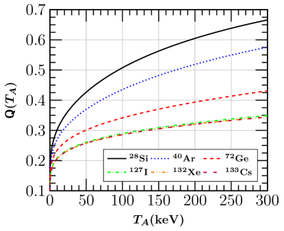
Figure 1: Quenching factor with respect to the nuclear recoil energy $T_{A}$ for the detector nuclei of the CE$\nu$NS experiments (see Table 1).

4.2 Neutrinos at the Spallation Neutron Source

The first CE$\nu$NS measurement by COHERENT became feasible by employing a CsI[Na] detector with mass $m_{\mathrm{det}}=14.57$ kg located at a baseline of $L=19.3$ m from the DAR-$\pi$ source with an exposure time of 308.1 days. Following the recipe of the COHERENT data release [17], we adequately simulate the DAR-$\pi$ neutrino spectra in terms of the pion and muon masses, $m_{\pi}$ and $m_{\mu}$, following the Michel spectrum [74]

$$f_{\nu_{\mu}}(E_{\nu}) =\delta\left(E_{\nu}-\frac{m_{\pi}^{2}-m_{\mu}^{2}}{2m_{\pi}}\right)\,,$$ (28)

$$f_{\bar{\nu}_{\mu}}(E_{\nu}) =\frac{64E^{2}_{\nu}}{m_{\mu}^{3}}\left(\frac{3}{4}-\frac{E_{\nu}}{m_{\mu}}\right)\,,$$

$$f_{\nu_{e}}(E_{\nu}) =\frac{192E^{2}_{\nu}}{m_{\mu}^{3}}\left(\frac{1}{2}-\frac{E_{\nu}}{m_{\mu}}\right)\,,$$

where $E_{\nu}^{\text{max}}\leq m_{\mu}/2\approx 52.8$ MeV. The latter accounts for the monochromatic muon neutrino beam ($E_{\nu}=29.9$ MeV) produced from pion decay at rest, $\pi^{+}\to\mu^{+}\nu_{\mu}$ (prompt flux with $\tau=26\,\mathrm{ns}$), and the subsequent $\nu_{e}$ and ${\bar{\nu}_{\mu}}$ neutrino beams resulting from muon decay $\mu^{+}\to\nu_{e}e^{+}\bar{\nu}_{\mu}$ (delayed flux with $\tau=2.2\,\mathrm{\mu s}$) [75]. The neutrino flux is $\Phi_{\nu}=rN_{\mathrm{POT}}/4\pi L^{2}$, with $r=0.08$ representing the number of neutrinos per flavor produced for each proton on target (POT), e.g. $N_{\mathrm{POT}}=1.76\times 10^{23}$ corresponding to the 308.1 days of exposure during the first run. For the future COHERENT detector subsystems HPGe, LAr and NaI[Tl], we assume an exposure period of 1 yr, which corresponds to $N_{\mathrm{POT}}=2.09\times 10^{23}$.

The COHERENT signal was detected through photoelectron (PE) measurements, hence, in our simulations we translate the energy of the scattered nucleus $T_{A}$ in terms of the number of the observed PE, $n_{\text{PE}}$, through the relation [16]

$$n_{\mathrm{PE}}=1.17\frac{T_{A}}{(\mathrm{keV})}\,,$$ (29)

taking also into consideration the photoelectron dependence of the detector efficiency $\mathcal{A}(x)$, required for determining the expected event rate below and given by [17]

$$\mathcal{A}(x)=\frac{k_{1}}{1+e^{-k_{2}\left(x-x_{0}\right)}}\Theta(x)\,,$$ (30)

with $k_{1}=0.6655$, $k_{2}=0.4942$, $x_{0}=10.8507$ and the Heaviside function

$$\Theta(x)=\left\{\begin{array}[]{ll}{0}&{x<5}\\ {0.5}&{5\leq x<6}\\ {1}&{x\geq 6\,.}\end{array}\right.$$ (31)

As in the case of reactor experiments, due to the lack of relevant information for the next generation detector subsystems HPGe, LAr and NaI[Tl], we assume a flat efficiency of $\mathcal{A}(T_{A})=0.5$.

5 Numerical Results

For a given CE$\nu$NS experiment, the total cross section is evaluated as a sum of the individual cross sections corresponding to each isotope composing the detector material. By taking into account the stoichiometric ratio of the atom, $\eta$, and the detector mass, $m_{\text{det}}$, the number of target nuclei per isotope is evaluated through Avogadro’s number, $N_{A}$

$$N_{\mathrm{targ}}^{x}=\frac{m_{\mathrm{det}}\eta_{x}}{\sum_{x}A_{x}\eta_{x}}N_{A}\,,$$ (32)

while the total number of events expected above threshold $T_{\mathrm{th}}$ (see Table 1) reads [64]

$$N_{\mathrm{theor}}=\sum_{\nu_{\alpha}}\sum_{x=\mathrm{isotope}}\mathcal{F}_{x}\int_{T_{\mathrm{th}}}^{T_{A}^{\mathrm{max}}}\int_{E_{\nu}^{\mathrm{min}}}^{E_{\nu}^{\mathrm{max}}}f_{\nu_{\alpha}}(E_{\nu})\mathcal{A}(T_{A})\left(\frac{{d\sigma}_{x}}{dT_{A}}(E_{\nu},T_{A})\right)_{\mathrm{tot}}dE_{\nu}dT_{A}\,,$$ (33)

where the luminosity for a detector with target material $x$ is given by $\mathcal{F}_{x}=N_{\mathrm{targ}}^{x}\Phi_{\nu}$ and $E_{\nu}^{\mathrm{min}}=\sqrt{m_{A}T_{A}/2}$ is the minimum incident neutrino energy to produce a nuclear recoil. Notice that we sum over all possible incident neutrino flavors $\alpha$ scattering off a detector with all possible isotopes $x$. It is worth mentioning that potential contributions to the event rate from detector dopants are safely ignored, since they are of the order $10^{-5}$ – $10^{-4}$ [76].

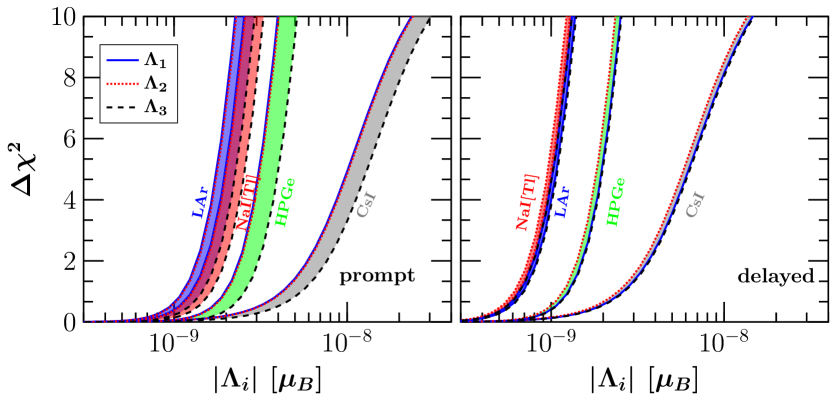
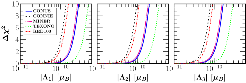
Figure 2: $\Delta\chi^{2}$ profiles for every element of the TMM matrix, $\left|\Lambda_{i}\right|$, at CE$\nu$NS experiments for vanishing $\left|\Lambda_{j}\right|$, $\left|\Lambda_{k}\right|$ and all phases set to zero. The results in the upper (lower) panel are for SNS (reactor) neutrino experiments in their current setup. The color bands in the upper panels indicate the limits expected from each SNS experiment.

In order to extract the current constraints on TMMs $\left|\Lambda_{i}\right|$ from the first phase of COHERENT (with a CsI detector), we perform a statistical analysis using the following $\chi^{2}$ function [16]

$$\chi^{2}(\mathcal{S})=\underset{\mathtt{a}_{1},\mathtt{a}_{2}}{\mathrm{min}}\Bigg{[}\frac{\left(N_{\mathrm{meas}}-N_{\mathrm{theor}}(\mathcal{S})[1+\mathtt{a}_{1}]-B_{0n}[1+\mathtt{a}_{2}]\right)^{2}}{(\sigma_{\mathrm{stat}})^{2}}+\left(\frac{\mathtt{a}_{1}}{\sigma_{\mathtt{a}_{1}}}\right)^{2}+\left(\frac{\mathtt{a}_{2}}{\sigma_{\mathtt{a}_{2}}}\right)^{2}\Bigg{]}\,.$$ (34)

Here, the measured number of events is $N_{\mathrm{meas}}=142$, while $\mathtt{a}_{1}$ and $\mathtt{a}_{2}$ are the systematic parameters accounting for the uncertainties on the signal and background rates, respectively, with fractional uncertainties $\sigma_{\mathtt{a}_{1}}=0.28$ and $\sigma_{\mathtt{a}_{2}}=0.25$. Following Ref. [16], the statistical uncertainty is given by $\sigma_{\mathrm{stat}}=\sqrt{N_{\mathrm{meas}}+B_{0n}+2B_{ss}}$, where the quantities $B_{0n}=6$ and $B_{ss}=405$ denote the beam-on prompt neutron and the steady-state background events respectively. Our statistical analysis regarding reactor as well as the next generation of COHERENT CE$\nu$NS experiments, within the framework of current and future setups, is based on a single nuisance parameter. In this case, the $\chi^{2}$ function is defined as

$$\chi^{2}(\mathcal{S})=\underset{\mathtt{a}}{\mathrm{min}}\Bigg{[}\frac{\left(N_{\text{meas}}-N_{\text{theor}}(\mathcal{S})[1+\mathtt{a}]\right)^{2}}{(1+\sigma_{\text{stat}})N_{\text{meas}}}+\left(\frac{\mathtt{a}}{\sigma_{\text{sys}}}\right)^{2}\Bigg{]}\,,$$ (35)

where we adopt the values $\sigma_{stat}=\sigma_{\text{sys}}=0.2$ $(0.1)$ for the current (future) setups. In order to probe TMMs, in what follows we perform a minimization over the nuisance parameter $\mathtt{a}$ and calculate $\Delta\chi^{2}(\mathcal{S})=\chi^{2}(\mathcal{S})-\chi^{2}_{\mathrm{min}}(\mathcal{S})$, with $\mathcal{S}\equiv\{\left|\Lambda_{i}\right|,\xi_{i},\delta_{\text{CP}}\}$ denoting the set of parameters entering the definition of the effective neutrino magnetic moment.

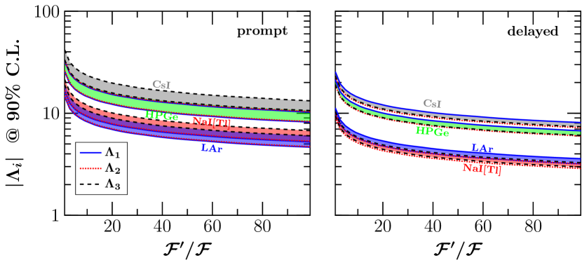
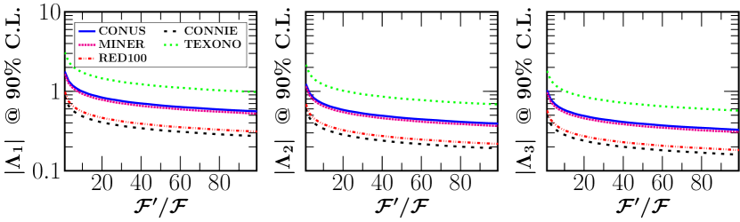
Figure 3: Variation of the 90% C.L. limits on $\left|\Lambda_{i}\right|$ as a function of the total luminosity $\mathcal{F^{\prime}}$ for SNS (upper panel) and reactor (lower panel) neutrino experiments. In all cases we assume vanishing $\left|\Lambda_{j}\right|$, $\left|\Lambda_{k}\right|$ and all phases set to zero. The results are shown in units $10^{-10}\mu_{B}$.

We begin our sensitivity analysis by considering a single non-vanishing TMM parameter $\left|\Lambda_{i}\right|$ at a time, in the current setup. As a first step, for the sake of simplicity, in our calculations we set all complex phases to zero, assuming all TMMs as real parameters. We will discuss the impact of non-zero phases on our reported sensitivities at the end of this section. The extracted constraints from the first CE$\nu$NS measurement in CsI along with the projected sensitivities from the next phase HPGe, LAr and NaI[Tl] COHERENT subsystems, are shown in the upper panel of Fig. 2 for prompt and delayed neutrinos. From the first run of the COHERENT experiment, the following 90% C.L. bounds are obtained from the prompt (delayed) neutrino beams

$$\left|\Lambda_{1}\right|< 69.2\,\,(54.5)\,\times 10^{-10}\,\mu_{B}\,,$$ (36)

$$\left|\Lambda_{2}\right|< 70.2\,\,(48.7)\,\times 10^{-10}\,\mu_{B}\,,$$

$$\left|\Lambda_{2}\right|< 89.6\,\,(49.8)\,\times 10^{-10}\,\mu_{B}\,.$$

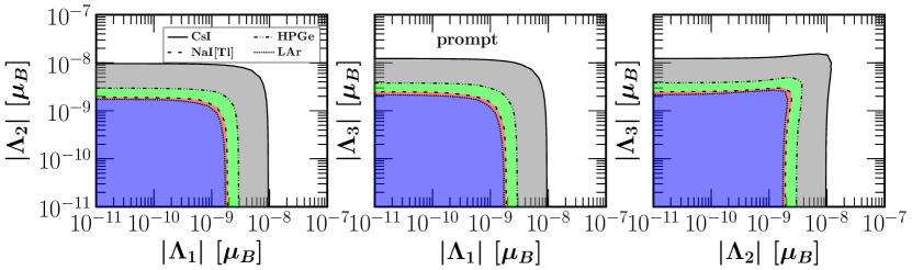
Figure 4: Regions in the $\left|\Lambda_{i}\right|-\left|\Lambda_{j}\right|$ parameter space allowed at 90% C.L. by current data of the COHERENT experiment (CsI detector) for vanishing values of the undisplayed $\left|\Lambda_{k}\right|$ and all phases. The upper (lower) panel presents the results for delayed (prompt) neutrinos in the current setup. We also display the projected sensitivities for the HPGe, LAr and NaI[Tl] detector subsystems of COHERENT. The color labeling is same as in Fig. 2.

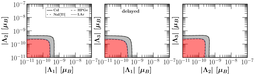
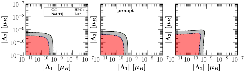
Figure 5: Same as Fig. 4 for the case of the future experimental setup at the SNS.

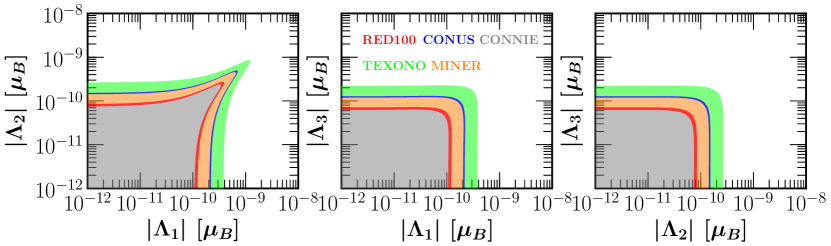
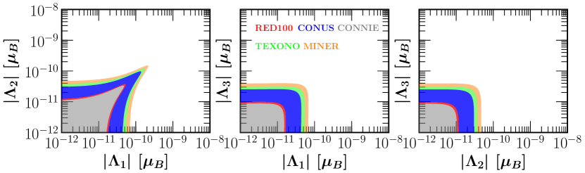
Figure 6: Projected 90% C.L. sensitivities in the $\left|\Lambda_{i}\right|-\left|\Lambda_{j}\right|$ plane assuming vanishing values of the undisplayed $\left|\Lambda_{k}\right|$ and CP phases. Upper and lower panels correspond to the current and future configurations of reactor neutrino experiments.

On the other hand, the lower panel of Fig. 2 presents the corresponding projected sensitivity from the reactor CE$\nu$NS experiments CONUS, CONNIE, MINER, TEXONO and RED100. The results presented in Fig. 2 indicate that the prospects for probing electromagnetic neutrino properties are better for reactor-based experiments. This is a direct consequence of their sub-keV recoil threshold capabilities in conjunction with the fact that the reactor neutrino energy distribution is peaked at much lower energies, compared to DAR-$\pi$ neutrinos. We stress, however, that when considering the full SNS beam, instead of the individual prompt and delayed components, this difference is reduced significantly. As an illustrative example, by assuming the full SNS beam in the current configuration of the CsI detector, the corresponding 90% C.L. upper bounds on ($\left|\Lambda_{1}\right|$, $\left|\Lambda_{2}\right|$, $\left|\Lambda_{3}\right|$) are (42.8, 40.0, 43.6) in units of $10^{-10}\,\mu_{B}$. Similarly, for the future detector materials of COHERENT, the projected sensitivities read, Ge: (16.5, 15.3, 16.6), LAr: (8.9, 8.4, 9.1) and NaI: (8.6, 8.0, 8.6), all in units of $10^{-10}\,\mu_{B}$.

For completeness, we now examine the attainable sensitivity for different values of the factor $\mathcal{F}$ which corresponds to the luminosity of each studied experiment, entering in the calculation of the event number in Eq. (33). To be conservative, we fix all other inputs to their default values according to the current setup and, as previously, we assume all TMMs to be real. We then calculate the sensitivities on $\left|\Lambda_{i}\right|$ for SNS and reactor CE$\nu$NS experiments by scaling-up our simulations with the new luminosity factor $\mathcal{F}^{\prime}$. With this approach, it becomes feasible to probe the sensitivity on TMMs for several combinations of detector mass, exposure period, detector baselines and power of the source. To motivate this approach, we recall that the SNS should increase its operation power and also that MINER is planning towards a moveable core strategy. Our corresponding results are depicted in Fig. 3. They show that there is a significant improvement by adopting scale-up factors of the order of $\mathcal{F}^{\prime}/\mathcal{F}\lesssim 40$, whereas beyond that point the improvement becomes weaker.

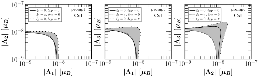
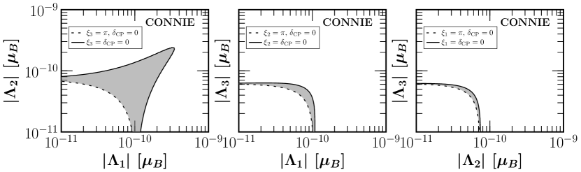
Figure 7: Projected 90% C.L. contours in the $\left|\Lambda_{i}\right|-\left|\Lambda_{j}\right|$ plane from the analysis of the prompt beam at the SNS (upper panel) and from the reactor neutrino experiment CONNIE (lower panel), for different values of the Majorana CP violating phases. As before, we have assumed a vanishing value for the undisplayed $\left|\Lambda_{k}\right|$.

We are now interested in exploring simultaneous constraints on the effective neutrino magnetic moment parameters from the current as well as projected CE$\nu$NS data, according to the setups reported in Table 1. Assuming two real non-vanishing TMMs at a time, in Fig. 4 we present the allowed regions in the $\left|\Lambda_{i}\right|-\left|\Lambda_{j}\right|$ plane extracted from the available CsI COHERENT data for the prompt and delayed beams. The corresponding regions for the next generation of COHERENT detectors are also shown. As can be seen from the plot, the installation of LAr and NaI[Tl] detector subsystems will offer improvements of about one order of magnitude, after one year of data taking. Figure 5 shows the projected sensitivities expected at various detector subsystems of COHERENT in the future setup, with an improvement of at least one order of magnitude. As commented above, a combined analysis of the full SNS beam, would have the potential to place even stronger limits. Turning now to reactor-based CE$\nu$NS experiments, we perform a similar analysis as previously described and present the projected sensitivities assuming the current (future) setup in the upper (lower) panel of Fig. 6. In both cases, the two-dimensional contour plots confirm that CE$\nu$NS experiments can be regarded as suitable facilities to probe Majorana electromagnetic properties with improved sensitivity. Indeed, as we will see in Sect. 6, with the next-generation upgrades, future measurements will have the potential to significantly improve upon the best current constraints, obtained from Borexino solar neutrino data. Finally, from Figs. 4-6, one sees that the resulting sensitivities have a slightly different shape in the $\left|\Lambda_{2}\right|-\left|\Lambda_{3}\right|$ plane compared to the other two panels for the case of SNS neutrinos. On the other hand, reactor neutrino experiments show a similar but more pronounced effect in the $\left|\Lambda_{1}\right|-\left|\Lambda_{2}\right|$ plane. This is due to its stronger dependence on the mixing angles and CP phases.

Before closing our discussion concerning the prospects of probing TMMs at CE$\nu$NS facilities, we examine the robustness of our results by exploring the impact of the CP phases on the derived sensitivities in the $\left|\Lambda_{i}\right|-\left|\Lambda_{j}\right|$ plane. As before, we assume a vanishing value for the remaining $\left|\Lambda_{k}\right|$. As an illustrative example, Fig. 7 shows the different 90% C.L. contours in the current setup obtained from the prompt beam at the COHERENT experiment (upper panel) and the projected reactor neutrino experiment CONNIE (lower panel). For SNS neutrinos, we have verified that the most conservative sensitivity (outer curve) corresponds to $\xi_{k}=0$ and $\delta_{\text{CP}}=\pi$, while the strongest one (inner curve) corresponds to $\xi_{k}=\pi$ and $\delta_{\text{CP}}=0$. On the other hand, for reactor neutrinos the most conservative sensitivity contour (outer curve) corresponds to $\xi_{k}=\delta_{\text{CP}}=0$, while the most aggressive one (inner curve) is obtained for $\xi_{k}=\pi$ and $\delta_{\text{CP}}=0$. All calculations refer to the current configuration, so that the solid lines correspond to the results presented in Figs. 4 and 6 assuming real TMMs.

6 Comparison with the current Borexino limit

As already discussed, the neutrino magnetic moment observable at a given experiment is actually an effective parameter depending on the neutrino mixing parameters as well as the oscillation factor describing the neutrino propagation between the source and detection points [69, 12], i.e.

$$\left(\mu^{M}_{\nu,\text{eff}}\right)^{2}(L,E_{\nu})=\sum_{j}\Big{|}\sum_{i}U^{\ast}_{\alpha i}e^{-i\,\Delta m^{2}_{ij}L/2E_{\nu}}\tilde{\lambda}_{ij}\Big{|}^{2}\,.$$ (37)

Note that, for the case of the short baseline CE$\nu$NS experiments discussed in the previous sections, the oscillation factor can be safely ignored, since there is no time for neutrino oscillations to develop.

To compare our results with current limits on TMMs, we analyze the recent solar neutrino data from Borexino phase-II [58] (see also Refs. [77, 78, 79]). In this case, the expression for the effective neutrino magnetic moment for solar neutrinos, in the mass basis is given by [49]

$$(\mu^{M}_{\nu,\,\text{sol}})^{2}=|\mathbf{\Lambda}|^{2}-c^{2}_{13}|\Lambda_{2}|^{2}+(c^{2}_{13}-1)|\Lambda_{3}|^{2}+c^{2}_{13}P^{2\nu}_{e1}(|\Lambda_{2}|^{2}-|\Lambda_{1}|^{2})\,,$$ (38)

where the oscillation probabilities from $\nu_{e}$ to the neutrino mass eigenstates $\nu_{i}$ have been approximated to [51]

$$P^{3\nu}_{e3}=\sin^{2}\theta_{13},\quad P^{3\nu}_{e1}=\cos^{2}\theta_{13}P^{2\nu}_{e1},\quad P^{3\nu}_{e2}=\cos^{2}\theta_{13}P^{2\nu}_{e2},\quad$$ (39)

and the unitarity condition, $P^{2\nu}_{e1}+P^{2\nu}_{e2}=1$, has been assumed . Notice that, in this case, Eq. (38) has no dependence on any phase, since solar electron neutrinos undergo flavor oscillations arriving to the detector as an incoherent admixture of mass eigenstates. In the recent analysis reported by the Borexino collaboration [58], the following 90% C.L. bound on the effective neutrino magnetic moment was reported: $\mu^{M}_{\nu,\,\text{sol}}<2.8\times 10^{-11}\mu_{B}$. This constraint can be directly translated into a limit on the TMM parameters $\left|\Lambda_{i}\right|$, as presented in Fig. 8. There, we show the corresponding 90% C.L. bounds in the two-dimensional ($\left|\Lambda_{i}\right|$,$\left|\Lambda_{j}\right|$) plane when the third element $\left|\Lambda_{k}\right|$ is set to zero.

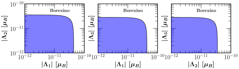
Figure 8: Regions in the $\left|\Lambda_{i}\right|-\left|\Lambda_{j}\right|$ plane allowed by Borexino solar data at 90% C. L. As before, we assume a vanishing value for the undisplayed $\left|\Lambda_{k}\right|$.

Before closing, it is worth mentioning that the effective neutrino magnetic moments can be also studied in other rare-event experiments. This is well-motivated by the improved precision expected in the next generation of oscillation and dark matter direct detection experiments, see Ref. [80]. In this framework, interesting neutrino sources such as geoneutrinos, atmospheric neutrinos and diffuse supernova background neutrinos that contribute to the “neutrino floor” at dark matter detectors can be envisaged. They would be expected to provide complementary information on neutrino electromagnetic properties.

7 Summary and Conclusions

Experiment	$\left|\Lambda_{1}\right|$	$\left|\Lambda_{2}\right|$	$\left|\Lambda_{3}\right|$
SNS prompt
CsI[Na]	69.2 [5.0]	70.2 [5.1]	89.6 [6.4]
HPGe	25.9 [5.1]	26.2 [5.2]	33.5 [6.6]
LAr	14.7 [2.9]	14.9 [2.9]	19.1 [3.7]
NaI[Tl]	16.6 [2.8]	16.8 [2.8]	21.5 [3.6]
SNS delayed
CsI[Na]	54.5 [4.2]	48.7 [3.7]	49.8 [3.7]
HPGe	21.3 [4.2]	18.9 [3.8]	19.1 [3.8]
LAr	11.3 [2.3]	10.1 [2.1]	10.4 [2.1]
NaI[Tl]	10.0 [2.3]	9.1 [2.0]	9.4 [2.0]
Reactor
CONUS	1.9 [0.37]	1.3 [0.26]	1.1 [0.22]
CONNIE	0.90 [0.13]	0.63 [0.09]	0.53 [0.08]
MINER	1.7 [0.58]	1.2 [0.41]	1.0 [0.34]
TEXONO	3.2 [0.46]	2.3 [0.32]	1.9 [0.27]
RED100	1.0 [0.14]	0.72 [0.10]	0.61 [0.08]
Solar
Borexino	0.44	0.36	0.28

Table 2: 90% C.L. limits on TMM elements $\left|\Lambda_{i}\right|$, in units of $10^{-10}$ $\mu_{B}$, from current and future CE$\nu$NS experiments. The numbers in square brackets indicate the attainable sensitivities in the future setups. Results from the solar neutrino experiment Borexino are also included for comparison.

In this work, we have examined the potential of the current and next generation of coherent elastic neutrino-nucleus scattering experiments in probing neutrino magnetic moment interactions. We have performed a detailed statistical analysis to determine the sensitivities on the three elements of the Majorana neutrino transition magnetic moment matrix, $\left|\Lambda_{i}\right|$, that follow from low-energy neutrino-nucleus experiments. We have used for the first time the CE$\nu$NS measurement by the COHERENT experiment at the Spallation Neutron Source in order to constrain the Majorana neutrino transition magnetic moments. By assuming the future setup upgrades in Table 1 we have also presented the expected sensitivities for the next phases of COHERENT using HPGe, LAr and NaI[Tl] detectors, as well as for reactor neutrino experiments such as CONUS, CONNIE, MINER, TEXONO and RED100. Our results for the current and future sensitivities on the TMM elements $\left|\Lambda_{i}\right|$ are illustrated in Figs. 2 to 6 and summarized in Table 2. From the table, one sees that improvements of at least one order of magnitude compared to the current setup might be expected from future CE$\nu$NS measurements. Indeed, our results show that the next generation CE$\nu$NS experiments has promising prospects to probe TMMs at the $10^{-11}\,\mu_{B}$ level at least. It follows that upcoming reactor-based CE$\nu$NS experiments with low-threshold capabilities have the potential to compete with the current limits from $\bar{\nu}_{e}-e$ scattering data derived in Ref. [49] or with the best current limit reported from Borexino, and translated to our general parameterization in Sect. 6 (see also the last row of Table 2). As a final remark, we comment that, although the results reported in Table 2 have been obtained under the assumption of real TMMs, we have also discussed the role of the CP violating phases.

- [1] T. Kajita, “Nobel Lecture: Discovery of atmospheric neutrino oscillations,” Rev. Mod. Phys. 88 no. 3, (2016) 030501.
- [2] A. B. McDonald, “Nobel Lecture: The Sudbury Neutrino Observatory: Observation of flavor change for solar neutrinos,” Rev. Mod. Phys. 88 no. 3, (2016) 030502.
- [3] D. V. Forero, M. Tortola, and J. W. F. Valle, “Global status of neutrino oscillation parameters after Neutrino-2012,” Phys. Rev. D86 (2012) 073012, arXiv:1205.4018 [hep-ph].
- [4] D. V. Forero, M. Tortola, and J. W. F. Valle, “Neutrino oscillations refitted,” Phys. Rev. D90 no. 9, (2014) 093006, arXiv:1405.7540 [hep-ph].
- [5] P. F. de Salas et al., “Status of neutrino oscillations 2018: 3 hint for normal mass ordering and improved CP sensitivity,” Phys. Lett. B782 (2018) 633–640, arXiv:1708.01186 [hep-ph].
- [6] J. Schechter and J. W. F. Valle, “Neutrino Masses in SU(2) x U(1) Theories,” Phys. Rev. D22 (1980) 2227.
- [7] J. Schechter and J. W. F. Valle, “Neutrino Decay and Spontaneous Violation of Lepton Number,” Phys. Rev. D25 (1982) 774.
- [8] J. Schechter and J. W. F. Valle, “Majorana Neutrinos and Magnetic Fields,” Phys. Rev. D24 (1981) 1883–1889. [Erratum: Phys. Rev.D25,283(1982)].
- [9] R. E. Shrock, “Electromagnetic Properties and Decays of Dirac and Majorana Neutrinos in a General Class of Gauge Theories,” Nucl. Phys. B206 (1982) 359.
- [10] B. Kayser, “Majorana Neutrinos and their Electromagnetic Properties,” Phys.Rev. D26 (1982) 1662.
- [11] J. F. Nieves, “Electromagnetic Properties of Majorana Neutrinos,” Phys. Rev. D26 (1982) 3152.
- [12] J. F. Beacom and P. Vogel, “Neutrino magnetic moments, flavor mixing, and the Super-Kamiokande solar data,” Phys. Rev. Lett. 83 (1999) 5222–5225, arXiv:hep-ph/9907383 [hep-ph].
- [13] M. Maltoni et al., “Status of global fits to neutrino oscillations,” New J.Phys. 6 (2004) 122, arXiv:hep-ph/0405172 [hep-ph]. this review gives a comprehensive set of references.
- [14] C. Broggini, C. Giunti, and A. Studenikin, “Electromagnetic Properties of Neutrinos,” Adv. High Energy Phys. 2012 (2012) 459526, arXiv:1207.3980 [hep-ph].
- [15] C. Giunti and A. Studenikin, “Neutrino electromagnetic interactions: a window to new physics,” Rev. Mod. Phys. 87 (2015) 531, arXiv:1403.6344 [hep-ph].
- [16] COHERENT Collaboration, D. Akimov et al., “Observation of Coherent Elastic Neutrino-Nucleus Scattering,” Science 357 no. 6356, (2017) 1123–1126, arXiv:1708.01294 [nucl-ex].
- [17] COHERENT Collaboration, D. Akimov et al., “COHERENT Collaboration data release from the first observation of coherent elastic neutrino-nucleus scattering,” arXiv:1804.09459 [nucl-ex].
- [18] M. Lindner, W. Rodejohann, and X.-J. Xu, “Coherent Neutrino-Nucleus Scattering and new Neutrino Interactions,” JHEP 03 (2017) 097, arXiv:1612.04150 [hep-ph].
- [19] J. Billard, J. Johnston, and B. J. Kavanagh, “Prospects for exploring New Physics in Coherent Elastic Neutrino-Nucleus Scattering,” arXiv:1805.01798 [hep-ph].
- [20] D. Aristizabal Sierra, V. De Romeri, and N. Rojas, “COHERENT analysis of neutrino generalized interactions,” Phys. Rev. D98 (2018) 075018, arXiv:1806.07424 [hep-ph].
- [21] O. G. Miranda, G. S. Garcia, and O. Sanders, “Testing new physics with future COHERENT experiments,” arXiv:1902.09036 [hep-ph].
- [22] J. Liao and D. Marfatia, “COHERENT constraints on nonstandard neutrino interactions,” Phys. Lett. B775 (2017) 54–57, arXiv:1708.04255 [hep-ph].
- [23] J. B. Dent, B. Dutta, S. Liao, J. L. Newstead, L. E. Strigari, and J. W. Walker, “Accelerator and reactor complementarity in coherent neutrino scattering,” arXiv:1711.03521 [hep-ph].
- [24] D. Aristizabal Sierra, N. Rojas, and M. H. G. Tytgat, “Neutrino non-standard interactions and dark matter searches with multi-ton scale detectors,” JHEP 03 (2018) 197, arXiv:1712.09667 [hep-ph].
- [25] P. B. Denton, Y. Farzan, and I. M. Shoemaker, “Testing large non-standard neutrino interactions with arbitrary mediator mass after COHERENT data,” JHEP 07 (2018) 037, arXiv:1804.03660 [hep-ph].
- [26] B. Dutta, S. Liao, S. Sinha, and L. E. Strigari, “Searching for Beyond the Standard Model Physics with COHERENT Energy and Timing Data,” arXiv:1903.10666 [hep-ph].
- [27] P. Coloma, M. C. Gonzalez-Garcia, M. Maltoni, and T. Schwetz, “COHERENT enlightenment of the neutrino dark side,” Phys. Rev. D96 no. 11, (2017) 115007, arXiv:1708.02899 [hep-ph].
- [28] M. C. Gonzalez-Garcia, M. Maltoni, Y. F. Perez-Gonzalez, and R. Zukanovich Funchal, “Neutrino Discovery Limit of Dark Matter Direct Detection Experiments in the Presence of Non-Standard Interactions,” JHEP 07 (2018) 019, arXiv:1803.03650 [hep-ph].
- [29] T. S. Kosmas et al., “Probing light sterile neutrino signatures at reactor and Spallation Neutron Source neutrino experiments,” Phys. Rev. D96 no. 6, (2017) 063013, arXiv:1703.00054 [hep-ph].
- [30] B. C. Cañas, E. A. Garcés, O. G. Miranda, and A. Parada, “The reactor antineutrino anomaly and low energy threshold neutrino experiments,” Phys. Lett. B776 (2018) 451–456, arXiv:1708.09518 [hep-ph].
- [31] C. Blanco, D. Hooper, and P. Machado, “Constraining Sterile Neutrino Interpretations of the LSND and MiniBooNE Anomalies with Coherent Neutrino Scattering Experiments,” arXiv:1901.08094 [hep-ph].
- [32] J. B. Dent, B. Dutta, S. Liao, J. L. Newstead, L. E. Strigari, and J. W. Walker, “Probing light mediators at ultralow threshold energies with coherent elastic neutrino-nucleus scattering,” Phys. Rev. D96 no. 9, (2017) 095007, arXiv:1612.06350 [hep-ph].
- [33] Y. Farzan, M. Lindner, W. Rodejohann, and X.-J. Xu, “Probing neutrino coupling to a light scalar with coherent neutrino scattering,” JHEP 05 (2018) 066, arXiv:1802.05171 [hep-ph].
- [34] M. Abdullah, J. B. Dent, B. Dutta, G. L. Kane, S. Liao, and L. E. Strigari, “Coherent Elastic Neutrino Nucleus Scattering (CENS) as a probe of through kinetic and mass mixing effects,” arXiv:1803.01224 [hep-ph].
- [35] V. Brdar, W. Rodejohann, and X.-J. Xu, “Producing a new Fermion in Coherent Elastic Neutrino-Nucleus Scattering: from Neutrino Mass to Dark Matter,” JHEP 12 (2018) 024, arXiv:1810.03626 [hep-ph].
- [36] S.-F. Ge and I. M. Shoemaker, “Constraining Photon Portal Dark Matter with Texono and Coherent Data,” arXiv:1710.10889 [hep-ph].
- [37] K. C. Y. Ng, J. F. Beacom, A. H. G. Peter, and C. Rott, “Solar Atmospheric Neutrinos: A New Neutrino Floor for Dark Matter Searches,” Phys. Rev. D96 no. 10, (2017) 103006, arXiv:1703.10280 [astro-ph.HE].
- [38] M. Cadeddu, C. Giunti, Y. F. Li, and Y. Y. Zhang, “Average CsI neutron density distribution from COHERENT data,” Phys. Rev. Lett. 120 no. 7, (2018) 072501, arXiv:1710.02730 [hep-ph].
- [39] D. K. Papoulias, T. S. Kosmas, R. Sahu, V. K. B. Kota, and M. Hota, “Constraining nuclear physics parameters with current and future COHERENT data,” arXiv:1903.03722 [hep-ph].
- [40] M. Cadeddu and F. Dordei, “Reinterpreting the weak mixing angle from atomic parity violation in view of the Cs neutron rms radius measurement from COHERENT,” Phys. Rev. D99 no. 3, (2019) 033010, arXiv:1808.10202 [hep-ph].
- [41] E. Ciuffoli, J. Evslin, Q. Fu, and J. Tang, “Extracting nuclear form factors with coherent neutrino scattering,” Phys. Rev. D97 no. 11, (2018) 113003, arXiv:1801.02166 [physics.ins-det].
- [42] M. Cadeddu, C. Giunti, K. A. Kouzakov, Y. F. Li, A. I. Studenikin, and Y. Y. Zhang, “Neutrino Charge Radii from COHERENT Elastic Neutrino-Nucleus Scattering,” Phys. Rev. D98 no. 11, (2018) 113010, arXiv:1810.05606 [hep-ph].
- [43] X.-R. Huang and L.-W. Chen, “Neutron Skin in CsI and Low-Energy Effective Weak Mixing Angle from COHERENT Data,” arXiv:1902.07625 [hep-ph].
- [44] D. Aristizabal Sierra, J. Liao, and D. Marfatia, “Impact of form factor uncertainties on interpretations of coherent elastic neutrino-nucleus scattering data,” arXiv:1902.07398 [hep-ph].
- [45] V. A. Bednyakov and D. V. Naumov, “Coherency and incoherency in neutrino-nucleus elastic and inelastic scattering,” Phys. Rev. D98 no. 5, (2018) 053004, arXiv:1806.08768 [hep-ph].
- [46] D. K. Papoulias, R. Sahu, T. S. Kosmas, V. K. B. Kota, and B. Nayak, “Novel neutrino-floor and dark matter searches with deformed shell model calculations,” Adv. High Energy Phys. 2018 (2018) 6031362, arXiv:1804.11319 [hep-ph].
- [47] C. Boehm, D. G. Cerdeno, P. A. N. Machado, A. O.-D. Campo, and E. Reid, “How high is the neutrino floor?,” JCAP 1901 (2019) 043, arXiv:1809.06385 [hep-ph].
- [48] J. M. Link and X.-J. Xu, “Searching for BSM neutrino interactions in dark matter detectors,” arXiv:1903.09891 [hep-ph].
- [49] B. C. Canas et al., “Updating neutrino magnetic moment constraints,” Phys. Lett. B753 (2016) 191–198, arXiv:1510.01684 [hep-ph].
- [50] M. Tortola, “Constraining neutrino magnetic moment with solar and reactor neutrino data,” PoS AHEP2003 (2003) 022, arXiv:hep-ph/0401135 [hep-ph].
- [51] W. Grimus et al., “Constraining Majorana neutrino electromagnetic properties from the LMA-MSW solution of the solar neutrino problem,” Nucl. Phys. B648 (2003) 376–396, arXiv:hep-ph/0208132 [hep-ph].
- [52] Private communication with conus collaboration.
- [53] CONNIE Collaboration, A. Aguilar-Arevalo et al., “Results of the engineering run of the Coherent Neutrino Nucleus Interaction Experiment (CONNIE),” JINST 11 no. 07, (2016) P07024, arXiv:1604.01343 [physics.ins-det].
- [54] MINER Collaboration, G. Agnolet et al., “Background Studies for the MINER Coherent Neutrino Scattering Reactor Experiment,” Nucl. Instrum. Meth. A853 (2017) 53–60, arXiv:1609.02066 [physics.ins-det].
- [55] H. T. Wong, “Neutrino-nucleus coherent scattering and dark matter searches with sub-keV germanium detector,” Nucl.Phys. A844 (2010) 229C–233C.
- [56] D. Y. Akimov et al., “RED-100 detector for the first observation of the elastic coherent neutrino scattering off xenon nuclei,” J. Phys. Conf. Ser. 675 no. 1, (2016) 012016.
- [57] COHERENT Collaboration, D. Akimov et al., “COHERENT 2018 at the Spallation Neutron Source,” arXiv:1803.09183 [physics.ins-det].
- [58] Borexino Collaboration, M. Agostini et al., “Limiting neutrino magnetic moments with Borexino Phase-II solar neutrino data,” Phys. Rev. D96 no. 9, (2017) 091103, arXiv:1707.09355 [hep-ex].
- [59] W. Grimus and T. Schwetz, “Elastic neutrino electron scattering of solar neutrinos and potential effects of magnetic and electric dipole moments,” Nucl. Phys. B587 (2000) 45–66, arXiv:hep-ph/0006028 [hep-ph].
- [60] B. C. Canas et al., “New limits on neutrino magnetic moments from low energy neutrino data,” J. Phys. Conf. Ser. 761 no. 1, (2016) 012043, arXiv:1609.08563 [hep-ph].
- [61] D. Z. Freedman, “Coherent neutrino nucleus scattering as a probe of the weak neutral current,” Phys. Rev. D9 (1974) 1389–1392.
- [62] D. K. Papoulias and T. S. Kosmas, “Standard and Nonstandard Neutrino-Nucleus Reactions Cross Sections and Event Rates to Neutrino Detection Experiments,” Adv. High Energy Phys. 2015 (2015) 763648, arXiv:1502.02928 [nucl-th].
- [63] P. Pirinen, J. Suhonen, and E. Ydrefors, “Neutral-current neutrino-nucleus scattering off Xe isotopes,” Adv. High Energy Phys. 2018 (2018) 9163586, arXiv:1804.08995 [nucl-th].
- [64] D. K. Papoulias and T. S. Kosmas, “COHERENT constraints to conventional and exotic neutrino physics,” Phys. Rev. D97 no. 3, (2018) 033003, arXiv:1711.09773 [hep-ph].
- [65] T. S. Kosmas et al., “Sensitivities to neutrino electromagnetic properties at the TEXONO experiment,” Phys. Lett. B750 (2015) 459–465, arXiv:1506.08377 [hep-ph].
- [66] J. Barranco, O. G. Miranda, and T. I. Rashba, “Probing new physics with coherent neutrino scattering off nuclei,” JHEP 12 (2005) 021, arXiv:hep-ph/0508299 [hep-ph].
- [67] Particle Data Group Collaboration, M. Tanabashi et al., “Review of Particle Physics,” Phys. Rev. D98 no. 3, (2018) 030001.
- [68] D. W. L. Sprung and J. Martorell, “The symmetrized fermi function and its transforms,” Journal of Physics A: Mathematical and General 30 no. 18, (Sep, 1997) 6525–6534. https://doi.org/10.1088%2F0305-4470%2F30%2F18%2F026.
- [69] P. Vogel and J. Engel, “Neutrino Electromagnetic Form-Factors,” Phys. Rev. D39 (1989) 3378.
- [70] T. S. Kosmas et al., “Probing neutrino magnetic moments at the Spallation Neutron Source facility,” Phys. Rev. D92 no. 1, (2015) 013011, arXiv:1505.03202 [hep-ph].
- [71] J. D. Lewin and P. F. Smith, “Review of mathematics, numerical factors, and corrections for dark matter experiments based on elastic nuclear recoil,” Astropart. Phys. 6 (1996) 87–112.
- [72] G. Mention, M. Fechner, T. Lasserre, T. A. Mueller, D. Lhuillier, M. Cribier, and A. Letourneau, “The Reactor Antineutrino Anomaly,” Phys. Rev. D83 (2011) 073006, arXiv:1101.2755 [hep-ex].
- [73] V. I. Kopeikin, L. A. Mikaelyan, and V. V. Sinev, “Spectrum of electronic reactor anti-neutrinos,” Phys. Atom. Nucl. 60 (1997) 172–176. [Yad. Fiz.60,230(1997)].
- [74] W. C. Louis, “Searches for muon-to-electron (anti) neutrino flavor change,” Prog. Part. Nucl. Phys. 63 (2009) 51–73.
- [75] Y. Efremenko and W. Hix, “Opportunities for Neutrino Physics at the Spallation Neutron Source (SNS),” J.Phys.Conf.Ser. 173 (2009) 012006, arXiv:0807.2801 [nucl-ex].
- [76] J. I. Collar, N. E. Fields, M. Hai, T. W. Hossbach, J. L. Orrell, C. T. Overman, G. Perumpilly, and B. Scholz, “Coherent neutrino-nucleus scattering detection with a CsI[Na] scintillator at the SNS spallation source,” Nucl. Instrum. Meth. A773 (2015) 56–65, arXiv:1407.7524 [physics.ins-det].
- [77] M. M. Guzzo, P. C. de Holanda, and O. L. G. Peres, “New limits on neutrino magnetic moment through nonvanishing 13-mixing,” Phys. Rev. D97 no. 9, (2018) 093006, arXiv:1212.1396 [hep-ph].
- [78] J. Barranco, D. Delepine, M. Napsuciale, and A. Yebra, “Distinguishing Dirac and Majorana neutrinos with astrophysical fluxes,” arXiv:1704.01549 [hep-ph].
- [79] A. N. Khan, “ estimate and neutrino electromagnetic properties from low-energy solar data,” J. Phys. G46 no. 3, (2019) 035005, arXiv:1709.02930 [hep-ph].
- [80] G.-Y. Huang and S. Zhou, “Constraining Neutrino Lifetimes and Magnetic Moments via Solar Neutrinos in the Large Xenon Detectors,” JCAP 1902 (2019) 024, arXiv:1810.03877 [hep-ph].