A catalog of known Galactic K-M stars of class I, candidate RSGs, in Gaia DR2.

Abstract

We investigate individual distances and luminosities of a sample of 889 nearby candidate red supergiants with reliable parallaxes ($\varpi/\sigma_{\varpi}>4$ and $\text{RUWE}<2.7$) from Gaia DR2. The sample was extracted from the historical compilation of spectroscopically derived spectral types by Skiff (2014), and consists of K-M stars that are listed with class I at least once. The sample includes well-known red supergiants from Humphreys (1978), Elias et al. (1985), Jura & Kleinmann (1990), and Levesque et al. (2005). Infrared and optical measurements from the 2MASS, CIO, MSX, WISE, MIPSGAL, GLIMPSE, and NOMAD catalogs allow us to estimate the stellar bolometric magnitudes. We analyze the stars in the luminosity versus effective temperature plane and confirm that 43 sources are highly-probably red supergiants with M_bol$<-7.1$ mag. 43% of the sample is made of stars with masses $>7$ M_⊙. Another $\approx$30% of the sample consists of giant stars.

1. Introduction

The Milky Way is the closest laboratory for resolved stellar populations and a prototype of spiral galaxies. Nonetheless our position within the disk and dust obscuration render its study difficult. Red supergiants (RSGs) are the brightest stars seen at infrared wavelengths, being young and cold objects with typical luminosity above $10^{4}$ L_⊙. RSGs are tracers of stellar populations from 4 to 30 Myr, with masses from about 9 to 40 M_⊙ (e.g. Ekström et al. 2012; Chieffi & Limongi 2013); from their numbers and luminosities one can evaluate Galactic star formation in this range of time. The distribution of known spectral types of Galactic RSGs peaks at spectral types M0–M2 (Elias et al. 1985; Davies et al. 2007).

Having said that, the current census of RSGs, including the M-types is highly incomplete, with little being known about their spatial distribution (see for example, Davies et al. 2009; Messineo et al. 2016). At optical wavelengths, catalogs of RSGs have been compiled by locating bright late-type stars in directions of OB associations. Humphreys (1978) lists 92 RSGs, Elias et al. (1985) list 90 RSGs, Levesque et al. (2005) analysed the spectra of 62 RSGs, Jura & Kleinmann (1990) list $\approx 135$ RSGs. Gehrz (1989) predicts at least 5000 RSGs. Overall, less than a thousand Galactic late-type stars of class I are known, with only about 400 RSGs. Their detection is extremely difficult since their colors are similar to those of giant late-type stars and knowledge on their distances is poor, and because their colours and magnitudes overlap with those of the more numerous Asymptotic giant branch (AGB) stars (from low masses to Super-AGBs of 9-10 M_⊙). Furthermore, even though associations and clusters make it easier to detect massive stars, it appears that only $\approx 2$% of inner Galaxy supergiants are associated with stellar clusters (Messineo et al. 2017). Pulsation properties and chemical abundances are required for identifying the stage of evolution and the nuclear burning that has occurred.

Gaia data allows us to classify individual stars by providing their distances. We prepared a catalog of bright late-type stars reported at least once with class I, i.e., as stars of K- or M-type and luminosity class I in the spectroscopic catalog of Skiff (2014), and with data from Gaia DR2. Historical spectroscopic records provided spectral types that in combination with Gaia parallaxes and photometric data enabled us to measure the stellar luminosities. With that in hand, we were able to extract a catalog of genuine stars of luminosity class I and to derive average magnitudes per spectral type. In Sect. 2, we describe the sample, their parallaxes, and available infrared measurements. In Sect. 3, we estimate the stellar luminosities and provide average values per spectral type. In Sect. 4, we summarize the results of our exercise.

2. Observational data

2.1. The sample and available spectral types

We compiled a list of about 1400 K-M stars of class I with latitudes $|b|<10^{\circ}$ from the historical records of stellar spectral types by Skiff (2014). All late-type stars with at least one classification as luminosity class I were retained. In addition, we cross-matched Skiff’s list with existing Galactic compilations of RSGs, for example by Humphreys (1978), Elias et al. (1985), Kleinmann & Hall (1986), Jura & Kleinmann (1990), Caron et al. (2003), Levesque et al. (2005), Figer et al. (2006), Davies et al. (2008), and Verhoelst et al. (2009). We also made use of the recent Galactic spectroscopic catalogues of bright late-type stars by Blum et al. (2003), Comerón et al. (2004), Clark et al. (2009), Liermann et al. (2009), Rayner et al. (2009), Negueruela et al. (2010), Negueruela et al. (2011), Verheyen et al. (2012), Dorda et al. (2016), Messineo et al. (2017), and Dorda et al. (2018). Sources with available spectral types and good parallaxes (see Sect. 2.2) are listed in Table 2. For sources listed in these recent catalogs, spectral classifications provided in the corresponding papers have been retained (see footnotes to Table 2). The catalog by Skiff (2014) collected spectroscopic classifications of Galactic stars available from the literature, with some entries dating back to 1930–1950. For each star from one to a dozen entries were available. For stars for which only one reference is given (that to Skiff’s database) we listed a spectral type range as well as the adopted spectral type, which is the mean (or most recent) of the measured spectral types.

2.2. Available parallaxes

Gaia data were taken from the recently released Gaia DR2 catalog (Gaia Collaboration et al. 2018, 2016), which contains $1.7$ billion sources. Typically, for parallaxes of stars brighter than $G=14$ mag, quoted uncertainties are about $0.04$ mas, $\approx 0.1$ mas for $G=17$ mag and $\approx 0.7$ mas for $G=20$ mag (see Luri et al. (2018)). Luminous late-type stars are characterised by brightness fluctuations due to convective motions and pulsation. The photocenters do not correspond to the stellar barycenters, but fluctuate around it (e.g., Chiavassa et al. 2011; Pasquato et al. 2011). This motion in general does not lead to systematic parallax errors, however, it degrades the goodness of fit of the astrometric solution (Chiavassa et al. 2011).

Initial celestial positions were taken from the catalog of Skiff (2014) and SIMBAD (Cambrésy et al. 2011) and improved with the positions of available 2MASS matches. Gaia matches were searched using a radius of 1$\farcs$5. This resulted in 1342 Gaia sources, providing matches for 96% of the initial sample of late-type stars.

For 7.5% of the sample parallaxes were available from both the Gaia DR2 and Hipparcos catalogs (ESA 1997); the mean difference of parallaxes is $0.08$ mas, with a dispersion around the mean of $1.21$ mas for stars with Gaia parallaxes larger than 2 mas.

2.2.1 Astrometric quality filtering and best sample

The goal of this work is to build a catalog of secure known K-M stars of class I, candidate RSGs, in Gaia DR2, and therefore to derive their average absolute magnitude for each spectral type. This means that here we calculate the luminosity of the candidate RSGs by direct integration of their stellar energy distribution (SED), independently of colours or other information that might be obtained from the spectral energy distribution. Hence, we rely on the Gaia DR2 parallax only to estimate the distances of the sources in our sample. In order to make sure the corresponding luminosity estimates are robust we will apply a rather conservative filtering on the quality of the parallax data, as described in the following.

Throughout the text we indicate with $\sigma_{\varpi}$ the external error of the parallax, which is defined as ${\sigma_{\varpi}}({\rm ext})=\sqrt{k^{2}\times{\sigma_{\varpi}}({\rm int})^{2}+\sigma_{s}^{2}}$, where ${\sigma_{\varpi}}({\rm int})$ is the internal error provided by DR2, and $k=1.08$ and $\sigma_{s}=0.021$ mas for $G<13$ mag (bright), and $k=1.08$ and $\sigma_{s}=0.043$ mas for $G\gtrsim 13$ (faint).

In order to select sources with good quality astrometry we analysed the $\varpi/\sigma_{\varpi}$ ratio and the so-called renormalized unit weight error (RUWE) which the Gaia team recommends to use instead of the filtering on the unit weight error described in appendix C of Lindegren et al. (2018). The RUWE can be calculated using lookup tables available from the ESA Gaia web pages and it is described in detail in a publicly available technical note (Lindegren et al. 2018). In Fig. 1 we show the RUWE as a function of $G$ for all the sources in our sample.

Stars for which $\varpi/\sigma_{\varpi}>4$ are indicated separately as well as stars for which no colour information is available (for which the value of the RUWE is less certain, this concerns 52 out of the 1342 sources in the sample). From this figure it is clear that most sources for which $\varpi/\sigma_{\varpi}>4$ have a RUWE value below $1.4$ (the threshold value recommended in Lindegren et al. 2018). A few stars with high signal to noise parallax values are located at $1.4<\text{RUWE}<2.7$. This suggests that a more relaxed filtering at $\text{RUWE}<2.7$ is adeguate for RSGs, so as to retain the brightest stars for which the RUWE values may be affected by photocenter motions.

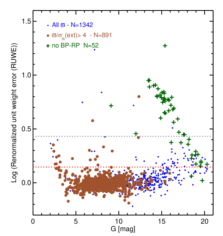
Figure 1.— The value of the RUWE vs. the apparent brightness in $G$ for all the source in our sample. The two lines indicate the limits $\text{RUWE}=1.4$ (in red) and $\text{RUWE}=2.7$ (in gray). The large brown dots indicate stars for which $\varpi/\sigma_{\varpi}$(ext)$>4$, while the dark-green crosses indicate stars for which no colour information is available from Gaia DR2.

We further restricted our sample to stars with $\varpi/\sigma_{\varpi}>4$ in order to ensure robust distance estimates. We motivate this in the next section. In the end we thus retained 889 sources with $\varpi/\sigma_{\varpi}>4$ and $\text{RUWE}<2.7$. The parallax range of the sources after filtering is $0.19$ to $7.53$ mas.

2.3. Distance estimates

The proper use of parallaxes in the distance estimation problem has been extensively reviewed in the context of Gaia DR2 by Luri et al. (2018). Their recommendation is not to use the inverse of the parallax as a distance indicator but to combine the parallax with other information and treat the estimation of distance as an inference problem. In our case we wish to use only the parallax in order to establish the luminosity of our stars independent from other information and in that case the Bayesian distance estimation method proposed by Bailer-Jones (2015), in particular using the exponentially decreasing space density prior, is a good choice (Luri et al. 2018). We will use the distances estimated by Bailer-Jones et al. (2018) for our selection of source with good quality and precise parallaxes, and motivate this as follows. For parallaxes with $\varpi/{\sigma_{\varpi}}({\rm ext})>4$ the Bailer-Jones et al. (2018) distances by design give essentially the same result as the $1/\varpi$ estimator, because for any reasonable length scale, $L$, of the exponentially decreasing space density prior the likelihood dominates the posterior on the distances. At larger relative parallax error, the prior plays a stronger role which would make our luminosity class estimates somewhat dependent on the Galactic model employed as a prior by Bailer-Jones et al. (2018). We verified that for our sources the relative differences between the $1/(\varpi-\varpi_{0})$ and Bailer-Jones et al. (2018) distance estimates are less than 5 per cent (see Fig. 2), with no trends as a function of the value of $L$. A summary of relative differences between the $1/(\varpi-\varpi_{0})$ and the Bailer’s distances ($R_{BJ})$ are provided in Table 1.

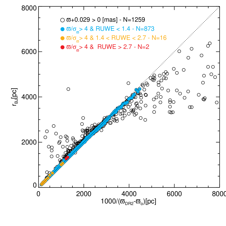
Figure 2.— Gaia data. Parallactic distances inferred with the Milky Way model by Bailer-Jones et al. (2018) versus parallactic distances from direct inversion of the parallaxes. Filled dots mark datapoints with $\varpi/{\sigma_{\varpi}}({\rm ext})>4$; in cyan those with $RUWE$ $<1.4$, in orange $1.4<$ $RUWE$ $\lesssim 2.7$, and in red $RUWE$ $>2.7$. The dotted line shows the points of the equation $r_{BJ}-(1000/(\varpi-\varpi_{o}))=0$ pc.

Table 1 Average difference of the distances provided by Bailer-Jones et al. (2018), $<R_{BJ}>$ and distances from direct inversion of the parallaxes for stars with $\varpi/{\sigma_{\varpi}}({\rm ext})>$ 2,3,4,5, and 10.

		All						$dist>3.5$ kpc
$\varpi/\sigma_{\varpi}$	$N_{\rm stars}$	$\Delta$(dist)	$\sigma$	$<\Delta$ (M1)$>$	$\sigma$	$<\Delta$ (M2)$>$	$\sigma$	$\Delta$(dist)	$\sigma$	$<\Delta$ (M1)$>$	$\sigma$	$<\Delta$ (M2)$>$	$\sigma$
		[pc]	[pc]	[mag]	[mag]	[mag]	[mag]	[pc]	[pc]	[mag]	[mag]	[mag]	[mag]
2	1075	$-$5.58	123.74	0.017	0.093	0.63	0.56	$-$289.04	316.95	$-0.13$	0.11	$0.96$	0.25
3	981	2.78	44.44	0.014	0.045	0.51	0.38	$-$124.94	105.35	$-0.06$	0.04	$0.82$	0.18
4	891	3.98	22.42	0.011	0.026	0.45	0.25	$\bf-83.72$	47.32	$\bf-0.05$	0.03	$\bf 0.70$	0.08
5	805	5.22	13.13	0.01	0.02	0.39	0.20	$-$58.394	23.28	$-0.03$	0.01	$0.62$	0.01
10	379	2.92	2.59	0.006	0.007	0.21	0.10	$..$	$..$

• Notes: $\Delta$(dist)$=<R_{BJ}-1000/(\varpi-\varpi_{0})>$. 
  $<\Delta(M1)>$ is the difference in the Distance Moduli inferred with the two distances $<R_{BJ}>$ and $<1000/(\varpi-\varpi_{0})>$. 
  $<\Delta(M2)>$ is the difference in the Distance Moduli of the high and low distances inferred by Bailer-Jones et al. (2018).
  

Using the distance estimates from Bailer-Jones et al. (2018) even for our sample with very precise parallaxes has the added advantage that the uncertainties on the distance estimates (as well as on the distance moduli used below) are well defined. On the contrary, the $1/\varpi$ distance estimator follows a probability distribution which cannot be normalised and thus has no expectation value or variance. Parallax uncertainties propagated into distance uncertainties ($\sigma_{d}\approx\sigma_{\varpi}/\varpi^{2}$) are thus formally meaningless for the $1/\varpi$ distance estimator (see Luri et al. 2018).

Table 2 Parallaxes and spectral types of the 889 stars with $\varpi/\sigma_{\varpi}>4$ and $\text{RUWE}<2.7$.

Gaia

Sptype

Distance

Cluster

Id

Alias

Ra(J2000)

Dec(J2000)

ID

$\varpi$

pmRa

pmDec

G

Vel∗

Sp(Skiff)

Sp(adopt)

Ref

Inv

MW

[hh mm ss]

[dd mm ss]

[mas]

[mas yr-1]

[mas yr-1]

[mag]

[km s-1]

[pc]

[pc]

1

${\rm PER002}$

0:00:18.123

60:21:01.538

423337510285997440

1.32$\pm$ 0.07

-6.831$\pm$ 0.081

-1.540$\pm$ 0.089

6.784$\pm$ 0.002

$..$

$..$

M4.5 Ib

4

743

744 ${}^{+33}_{-31}$

$..$

2

${\rm PER006}$

0:02:59.105

61:22:05.344

429500547840721536

0.98$\pm$ 0.04

-1.181$\pm$ 0.059

-1.221$\pm$ 0.056

8.490$\pm$ 0.001

-45.580$\pm$ 0.190

$..$

M3 Ib

4

990

992 ${}^{+36}_{-34}$

$..$

3

${\rm PER008}$

0:06:38.571

58:02:18.208

422677631507971840

0.82$\pm$ 0.08

-3.328$\pm$ 0.099

-3.282$\pm$ 0.089

9.598$\pm$ 0.002

$..$

$..$

M5 Ib

4

1176

1183 ${}^{+117}_{-98}$

$..$

4

${\rm PER010}$

0:09:26.327

63:57:14.090

431678852171577216

0.40$\pm$ 0.07

-3.633$\pm$ 0.098

-0.372$\pm$ 0.110

6.768$\pm$ 0.012

-54.300$\pm$ 0.530

$..$

M2 Iab

4

2350

2355 ${}^{+423}_{-314}$

$..$

5

${\rm KN~{}Cas}$

0:09:36.363

62:40:04.091

429999760479435520

0.29$\pm$ 0.06

-1.850$\pm$ 0.077

-1.817$\pm$ 0.059

8.356$\pm$ 0.002

$..$

$..$

M1 Ib

1,5,9

3131

3082 ${}^{+558}_{-416}$

Cas OB5

6

${\rm PER012}$

0:12:21.655

62:53:33.738

431331097263392384

0.95$\pm$ 0.04

-1.455$\pm$ 0.043

-2.351$\pm$ 0.044

6.914$\pm$ 0.000

-35.120$\pm$ 0.150

$..$

K0 Iab

1,4

1025

1026 ${}^{+29}_{-27}$

$..$

7

${\rm PER015}$

0:15:01.100

66:06:50.122

528168213046737024

2.16$\pm$ 0.04

5.334$\pm$ 0.048

-5.527$\pm$ 0.046

7.231$\pm$ 0.001

-32.050$\pm$ 0.180

$..$

K3 Ib

4

456

456 ${}^{+7}_{-7}$

$..$

8

${\rm PER019}$

0:18:26.380

60:54:09.149

428817510598195584

0.42$\pm$ 0.04

-2.826$\pm$ 0.049

-1.200$\pm$ 0.044

7.795$\pm$ 0.001

-49.280$\pm$ 0.170

$..$

M1 Iab

4

2222

2220 ${}^{+165}_{-144}$

$..$

9

${\rm PER022}$

0:20:43.560

61:52:46.537

430464235421496320

0.81$\pm$ 0.09

-1.599$\pm$ 0.104

-0.334$\pm$ 0.094

5.760$\pm$ 0.002

-29.740$\pm$ 0.320

$..$

M1 Iab

4,8

1188

1198 ${}^{+130}_{-107}$

$..$

10

${\rm BD~{}+59~{}38}$

0:21:24.278

59:57:11.155

428379733171150336

0.53$\pm$ 0.07

-3.470$\pm$ 0.084

-0.924$\pm$ 0.070

7.966$\pm$ 0.005

-55.570$\pm$ 0.850

$..$

M2/M2 Iab/I

1,2,5,8,9

1778

1783 ${}^{+230}_{-184}$

Cas OB4

• Notes: The identification number (Id) is followed by an Alias name, the Gaia coordinates, the Gaia parameters (name=ID, parallax=$\varpi$ and its external error ($\sigma_{\varpi}$), proper motions, $G$-band magnitude, Vel), the spectral types (Sp(Skiff)) collected by Skiff (2014), the adopted spectral type (Sp(adopt)), references for the spectral types (Ref), distances, and nearby clusters.
  Sp(adopt) is that of the first reference listed which is $\neq 1$. When only Skiff’s reference is present (=1), an average spectral type from Skiff’s records is adopted and the encountered spectral range is annotated (Sp(Skiff)). When Levesque et al. (2005) reference is present (=2), two values are provided, the photographic MK type and class, and the new type by Levesque et al. (2005) (revised by fitting synthetic models).
  ”Inv” distances are obtained by inversion of the parallaxes, ”MW” distances and relative errors are those of Bailer-Jones et al. (2018), and are based on a prior derived from a Milky Way model.
  (^∗) Spectroscopic radial velocity in the solar barycentric reference frame.
  

• References: 2=Levesque et al. (2005); 3= Verhoelst et al. (2009); 4=Dorda et al. (2018); 5= Dorda et al. (2016); 6=Kleinmann & Hall (1986); 7=Elias et al. (1985); 8=Jura & Kleinmann (1990); 9=Humphreys (1978); 10=Messineo et al. (2017); 11=Messineo et al. (2014); 12=Negueruela et al. (2012); 13=Negueruela et al. (2011); 14=Rayner et al. (2009); 15=Liermann et al. (2009); 16=Mermilliod et al. (2008); 17=Messineo et al. (2008); 18=Mengel & Tacconi-Garman (2007); 19=Caron et al. (2003); 20=Massey et al. (2001); 21=Eggenberger et al. (2002). 
  

2.3.1 RSGs related to clusters and radio parallaxes

In this work, we treated the stars individually. However, in Table 2 we have annotated possible associations with known clusters, which is based on current literature. Only 13% of the sample was found associated. Memberships are not the focus of this work as they require an extensive and careful revision of each open cluster. For example, with Gaia DR2 data doubt is cast even upon the association of $\eta$ Car with the young cluster Trumpler 16 (Davidson et al. 2018).

The 22 RSGs reported in Table 2 as associated to the Per OB1 association yield an average $\varpi+0.029=0.51$ mas with a dispersion around the mean of $0.13$ mas, or an average $\varpi+0.029=0.54$ mas with a dispersion of $0.11$ mas when including only the best quality sources. The annual parallax of maser spots measured toward S Persei is $0.413\pm 0.017$ mas (Asaki et al. 2010). Unfortunately, the Gaia parallax of S Persei (G=7.80 mag) has a large uncertainty, $\varpi=0.22\pm 0.13$ mas, RUWE=1.27, $\varpi/{\sigma_{\varpi}}({\rm ext})$=1.67.

Zhang et al. (2012) and Choi et al. (2008) reported on astrometric observations of $H_{2}O$ masers around the red supergiant VY Canis Majoris ($G=7.17$ mag). The trigonometric parallax is $0.88\pm 0.08$ mas, corresponding to a distance of $1.14^{0.11}_{-0.09}$ kpc. Unfortunately, Gaia measurements are highly uncertain ($\varpi=-5.92\pm 0.89$ mas, RUWE=17.19).

The red hypergiant VX Sgr ($G=7.17$ mag) has a trigonometric parallax of $0.64\pm 0.04$ mas, corresponding to a distance of $1.56_{-0.10}^{+0.11}$ kpc (via water maser observations, Xu et al. 2018). Chen et al. (2007) had estimated a distance of $1.57\pm 0.27$ kpc with SiO maser observations. Gaia parallax is $\varpi=0.79\pm 0.27$ mas, $1.36^{+1.02}_{-0.41}$ kpc (RUWE=1.96, $\varpi/{\sigma_{\varpi}}({\rm ext})$=3.17). VX Sgr remains outside of our selected 889 stars because of its low $\varpi/\sigma_{\varpi}$, however, the radio parallax and Gaia parallax agree within 23%.

The red supergiant PZ Cas ($G=6.64$ mag) has an annual parallax of $0.356\pm 0.026$ mas, corresponding to a distance of $2.81^{+0.22}_{-0.19}$ kpc (from water maser observations, Kusuno et al. 2013). Gaia measurements are consistent within errors ($\varpi=0.42\pm 0.09$ mas, $2.22^{+0.53}_{-0.36}$ kpc, RUWE=1.06, $\varpi/{\sigma_{\varpi}}({\rm ext})$=4.67). PZ Cas is listed in Table 2. The radio and Gaia parallaxes agree within 18%.

2.4. Photometric catalog

Photometric $JH$K_s measurements from the Two Micron All Sky Survey (2MASS) catalog (Skrutskie et al. 2006; Cutri et al. 2003) were available for 97% of the sample in Table 2. Their K_s values range from $-4$ mag to about 12.5 mag. Of the K_s magnitudes 43% are brighter than K_s$=4$ mag, and magnitudes are based on the fitting of the wing of the PSF on the 51ms exposures (red flag Rk = 3, see Table 2). For 6.5% of these stars, we were also able to retrieve $J$, $H$, and $K$ measurements in the Catalog of Infrared Observations, CIO 5th edition, by Gezari et al. (1996); the average difference at 2 $\mu$m is $0.13$ mag with $\sigma=0.14$ mag. For the remaining 2.7% of the sample with missing near-infrared measurements, we used the photometry of Morel & Magnenat (1978), Liermann et al. (2009), Messineo et al. (2010), and Stolte et al. (2015). For the faintest star OGLE BW3 V 93508 ($K=13.9$ mag) the measurements are from Lucas et al. (2008).

For 78% of the stars mid-infrared measurements from the Midcourse Space Experiment (MSX, Egan et al. 2003; Price et al. 2001) were available. For 27% of the sample 24 $\mu$m measurements from MIPSGAL by Gutermuth & Heyer (2015) were available. For 32% of the sample there were GLIMPSE measurements (Churchwell et al. 2009; Benjamin et al. 2005); for 96% mid-infrared measurements from 3.6 $\mu$m to 22 $\mu$m were available from the Wide-field Infrared Survey Explorer (WISE) (Wright et al. 2010). We used an initial search radius of 5^′′ and selected the closest matches. The MSX matches were at an average distance of 1$\farcs$3 with $\sigma$=0$\farcs$9 from the 2MASS positions; the WISE matches at an average distance of 0$\farcs$4 ($\sigma$=0$\farcs$4). The Gaia positions were searched to within 1$\farcs$5 of the 2MASS positions, and have an average displacement of 0$\farcs$17 and a $\sigma$=0$\farcs$13 from the 2MASS centroids; 2MASS stars are the closest matches to the Gaia sources and also the brightest K_s sources. Matches were confirmed with a visual inspection of 2MASS and WISE images, as well as of the stellar energy distribution (SED). Notes on the matches are provided in Appendix A.

$BVR$ photometry was retrieved from The Naval Observatory Merged Astrometric Dataset (NOMAD) (Zacharias et al. 2005). The photometric data for the subsample of 889 stars with good parallaxes are listed in Table 3.

Table 3 Infrared measurements of the bright late-type stars in Table 2.

	2MASS∗									CIO			GLIMPSE				MSX				WISE				MIPS	NOMAD			Nstar+
ID	J	Rj	Qj	H	Rh	Qh	$K_{S}$	Rk	Qk	J	H	K	[3.6]	[4.5]	[5.8]	[8.0]	A	C	D	E	W1	W2	W3	W4	[24]	B	V	R
	1.2			1.6			2.2			1.25	1.65	2.20	3.6	4.5	5.8	8.0	8.3	12.1	14.6	21.3	3.4	4.6	11.6	22.1	23.7
	[mag]			[mag]			[mag]			[mag]	[mag]	[mag]	[mag]	[mag]	[mag]	[mag]	[mag]	[mag]	[mag]	[mag]	[mag]	[mag]	[mag]	[mag]	[mag]	[mag]	[mag]	[mag]
1	3.56	3	D	2.64	3	C	2.18	3	D	$..$	$..$	$..$	$..$	$..$	$..$	$..$	1.87	1.86	1.62	$..$	$..$	$..$	1.97	1.79	$..$	10.15	8.48	7.60	110
2	5.53	1	A	4.62	1	A	4.30	1	A	$..$	$..$	$..$	$..$	$..$	$..$	$..$	4.17	$..$	$..$	$..$	4.19	4.05	4.21	4.06	$..$	11.49	9.75	8.87	110
3	5.81	1	A	4.86	1	E	4.48	1	A	$..$	$..$	$..$	$..$	$..$	$..$	$..$	4.30	$..$	$..$	$..$	4.37	4.32	4.29	4.11	$..$	16.46	$..$	10.50	110
4	3.21	3	D	2.15	3	D	1.73	3	D	$..$	$..$	1.81	$..$	$..$	$..$	$..$	0.17	-0.42	-0.39	-1.18	$..$	$..$	-0.23	-1.22	$..$	10.22	8.37	7.49	110
5	5.25	1	A	4.53	3	D	4.29	3	D	$..$	$..$	$..$	$..$	$..$	$..$	$..$	3.74	3.60	$..$	$..$	3.80	3.68	3.73	3.53	$..$	11.30	9.57	8.69	110
6	5.03	3	D	4.08	3	D	3.64	1	E	$..$	$..$	$..$	$..$	$..$	$..$	$..$	3.48	3.44	$..$	$..$	3.53	3.40	3.55	3.47	$..$	9.25	7.55	6.67	110
7	4.53	3	D	3.66	3	C	3.36	3	D	$..$	$..$	$..$	$..$	$..$	$..$	$..$	3.27	3.39	$..$	$..$	$..$	3.25	3.34	3.23	$..$	10.11	8.20	7.32	110
8	4.79	3	D	3.74	3	D	3.25	3	D	$..$	$..$	$..$	$..$	$..$	$..$	$..$	2.98	2.77	2.69	$..$	$..$	3.06	2.99	2.60	$..$	11.41	9.10	8.53	110
9	3.12	3	D	2.26	3	C	1.88	3	D	$..$	$..$	1.75	$..$	$..$	$..$	$..$	1.53	1.44	1.37	1.45	$..$	$..$	1.65	1.48	$..$	8.82	6.85	5.97	110
10	4.58	3	D	3.43	3	D	2.71	3	D	$..$	$..$	$..$	$..$	$..$	$..$	$..$	0.97	0.28	0.45	-0.12	$..$	$..$	0.50	-0.12	$..$	11.82	9.66	8.94	110

• Notes: The identification number (Id) is followed by the 2MASS $JHK$ measurements with corresponding red flags (Rj,Rh,Rk) and quality flags (Qj,Qh,Qk), CIO $JHK$ magnitudes, MSX $A,C,D,E$ magnitudes, WISE $W1,W2,W3,W4$ magnitudes, MIPS 24 $\mu$m magnitude, the NOMAD $BVR$ magnitudes, and the Nstar value. 
  (⁺) Nstar=XYZ, where X=number of MSX detected within the search radius; Y= number of WISE stars within the search radius; Z= number of GLIMPSE stars with 8 $\mu$m magnitudes $<10$ within the search radius. A value equals to 9 indicates that the counter is not available. 
  (^∗)If the 2MASS quality flags are equal to ’M’ the measurements have other origins as specified in Appendix A. 
  A few WISE and MSX measurements were discarded (Appendix A).

3. Luminosities

3.1. Bolometric magnitudes

We estimated the stellar luminosities using the photometric measurements, an extinction power law with an index of 1.9 (Messineo et al. 2005), and the distance moduli derived from the Gaia parallaxes. For spectral types from K0 to M5, intrinsic $J-$K_s and $H-$K_s colours were taken from Koornneef (1983). For M6–M9 types intrinsic colours were derived from the colours of giants (e.g. Koornneef 1983; Montegriffo et al. 1998; Cordier et al. 2007) and the average offset between the colours of giants and supergiants of types M3–M5 were applied. Bolometric corrections to the absolute $K$-magnitudes were provided by Levesque et al. (2005). In addition to this calculation, we performed a direct flux integration using the $JH$K_s measurements, and the mid-infrared measurements from MSX, WISE, GLIMPSE, and MIPSGAL. Measurements were dereddened with extinction ratios as described in Messineo et al. (2005). The integral under the stellar energy distribution (SED) was estimated with the trapezium method; flux extrapolations at the red-extremes were performed with a linear interpolation passing through the last reddest data-point and going to zero flux at 500 $\mu$m, while at the blue-extreme (bluer than $J$-band) we use a black body extrapolation (see Messineo et al. 2017). Red extrapolation contains about 5‰ of the flux. The average difference between the M_bol calculated with the BC${}_{K_{\rm S}}$ and those calculated by integrating under the SED is 0.05 mag with a $\sigma$=0.18 mag. Inferred M_bol values are listed in Table 6.

We estimated de-reddened $BV$ photometry, $V_{\rm o}$ and $B_{\rm o}$, by using the estimated A${}_{K_{\rm s}}$ and assuming $R=3.1$ and the extinction ratios in Messineo et al. (2005).

3.2. Luminosity classes and nuclear burnings

The MK system was established in 1943 by Morgan and Keenan, and it is an empirical system for the stellar spectral classification. It is based on a known atlas of standard stars with spectral types and luminosity classes (Morgan et al. 1943). Stellar spectra are classified by direct comparison with spectra of standard stars observed at the same resolution and with the same instrument. Through quantitative spectral analysis one can estimate gravity, $g$, or T_eff, however, such quantities are external to the definition of MK system itself. While spectroscopic indicators of luminosity for dwarfs and evolved late-type stars are at our disposal from atomic lines and molecular bands, the separation of giants and supergiants remains difficult. Furthermore, spectroscopic optical and infrared classifications may provide somewhat different results (Gray & Corbally 2009); supplementary information on distances, luminosities, and chemical composition is necessary.

Higher extinction renders the $M_{V}$ versus $B_{\rm o}-V_{\rm o}$ unsuitable for studies of the inner Galaxy, and it is useful to translate the optical quantities into infrared quantities and theoretical quantities. Furthermore, it is useful to look at these diagrams by keeping in mind which types of nuclear burnings may occur.

AGBs and RSGs are cold objects with similar ranges of effective temperatures, therefore spectral types. They overlap in luminosity. AGB stars can even be brighter than RSGs, and it is not known apriori from the luminosity classes the type of internal nuclear burnings and neither their distances.

AGB stars are stars of low or intermediate masses ($\lesssim 9$ Msun) burning helium and hydrogen in shells, with a degenerate core of CO. AGB stars from 6.5 to 9.5 M_⊙  experience off-center nuclear burnings and from 9 to 10 M_⊙ can even reach iron core state and evolve into neutron star.

As Iben (1974) writes, massive stars are stars which do not develop a strongly electron-degenerate core until all exoergic reactions have run to completion at the center. RSGs are massive stars from $\approx 9$ to $\approx 40$ M_⊙ (Ekström et al. 2012). Most of them are burning He when they reach the RSG phase. For a RSG of 9 M_⊙  models predict M_bol from $-4.5$ to $-6.8$ mag and spectral types from K0 to M4.5, while for a RSG of 25 M_⊙, M_bol $\approx-8.8$ mag and spectral type K5 (see Table 4). Observations closely follow the new evolutionary tracks by Ekström et al. (2012). The M_bol values of the $\approx 90$ Galactic RSGs recently analysed by Levesque et al. (2005) range from M_bol=$-3.63$ mag to M_bol= $-10.36$ mag.

A few observational luminosity benchmarks of late-type stars of low and intermediate masses are here useful. The tip of red giant branch stars in Galactic globular clusters occurs at M_bol = $-3.6$ to $-3.8$ mag in metal-rich globular clusters, such us 47 Tuc (e.g. Ferraro et al. 2000); members brighter than that are thermally pulsing TP-AGBs. The maximum luminosity that more massive AGB stars can reach is about $-7.1$ mag (Vassiliadis & Wood 1993). Very massive AGB stars may experience hot-bottom burning which further increases their luminosity, but this phenomenon primarily affects metal poor populations and is thus expected to only moderately affect the Milky Way disk population. The latest models of Doherty et al. (2015) predict that a super-AGB of 9 M_⊙ would reach M_bol$=-7.6$ mag. Therefore, AGBs do have a large overlap in luminosity with RSGs, and may enter the luminosity classes Ia, Ib, and Ib-II; for example, as pointed out by the kind referee, $\alpha$ Her is an AGB of 2–3 M_⊙ with class Ib-II (Moravveji et al. 2013), and NGC6067 hosts several AGBs of 6 M_⊙ with types K0-K4 and classes Iab-Ib, Iab-Ib and Ib (Alonso-Santiago et al. 2017).

However, observationally, we can see that field AGB stars in the Baade’s Windows with M_bol from $\approx-5.0$ to $-7.1$ mag are large amplitude pulsators (Miras) (e.g. Alard et al. 2001), and generally have late-$M$ spectral types, M4-M9 (i.e. T_eff cooler than 3500 K, Alard et al. 2001; Blanco et al. 1984); similarly, the 4 Mira stars (V1-V4) at the tip of the red branch of the globular cluster 47 Tuc have spectral types M4-M5 (Glass & Feast 1973; Skiff 2014). By contrast, semiregular AGB pulsators are typically fainter than Mira AGBs: $-2.5\gtrsim$ M_bol$\gtrsim-5.0$ mag, while Miras have $-3.6\gtrsim$ M_bol$\gtrsim-7$ mag (e.g., Alard et al. 2001).

In conclusion, only stars brighter than M_bol$\approx-7.5$ mag (masses $>15$ M_⊙) are certain RSGs; late-type stars earlier than $M4$ and with M_bol$\lesssim-5.0$ mag are expected to have masses $\gtrsim 5-7$ M_⊙. For field late-type stars fainter or redder than that, AGB stars are the dominant population when M_bol$<-3.6$ mag (see Table 4).

Table 4 Summary of M_bol and temperatures of Galactic massive cool stars (RSGs) and other cool stars of low and intermediate masses.

Mass	Age_to_red	T_red	Phase	Mbol	Teff	Sp. Type	Comments
M⊙	[Myr]	[Myr]		[mag]	[K]
0.6-0.8			tip-rgb	[$-3.6$,$-3.8$]			Observed range in globular clusters (Ferraro et al. 2000)
1.35-1.7			tip-rgb	[3.4]			Rot. tracks by Ekström et al. (2012)
$<2.0-2.8$			tip-rgb	[$-3.5$,$-3.7$]			He-flash theory for Z=0.01 (Sweigart et al. 1990)
			AGB-Mira	[$-5.0$,$-7.1$]			Observed bulge stars in Alard et al. (2001)
			AGB-Mira		$<3500$	M4-M9	Observed range in the Bulge (Blanco et al. 1984)
0.85c	11.8c		AGB-Mira		$<3500$	M4-M5	Observed range in old 47 Tuc (Glass & Feast 1973; Skiff 2014)
			AGB-SR	[$-2.5$,$-5.0$]			Observed. Bulge stars in Alard et al. (2001)
1	11250	12	AGB	$[-3.61,-4.03]$			Mbol during E-AGB and TP-AGB by Vassiliadis & Wood (1993)
2	1236	9	AGB	$[-3.78,-4.90]$			Mbol during E-AGB and TP-AGB by Vassiliadis & Wood (1993)
3.5	230	3	AGB	$[-5.17,-5.65]$			Mbol during E-AGB and TP-AGB by Vassiliadis & Wood (1993)
5	95	1.4	AGB	$[-5.91,-6.22]$			Mbol during E-AGB and TP-AGB by Vassiliadis & Wood (1993)
7			S-AGB	[$-6.86$]			minimum Mbola Doherty et al. (2015)
8			S-AGB	[$-7.20$]			minimum Mbola Doherty et al. (2015)
9			S-AGB	[$-7.60$]			minimum Mbola Doherty et al. (2015)
9.8			S-AGB	[$-7.86$]			minimum Mbola Doherty et al. (2015)
3	417		S-AGB	[$-0.3$,$-1.7$]	4850 - 4300	$>$K0	Rot. tracksb by Ekström et al. (2012)
5	111		S-AGB	[$-2.3$,$-4.4$]	4600 - 3800	$>$K0 - M0	Rot. tracksb by Ekström et al. (2012)
7	52		S-AGB	[$-3.5$,$-5.9$]	4400 - 3550	$>$K0 - M3.5	Rot. tracksb by Ekström et al. (2012)
9	32	3.7	RSG	[$-4.5$,$-6.8$]	4200 - 3500	K0 - M4.5	Rot. tracks by Ekström et al. (2012)
12	20	2.0	RSG	[$-6.0$,$-7.4$]	3900 - 3550	K4 - M3.5	Rot. tracks Ekström et al. (2012)
15	12.5	1.0	RSG	[$-7.3$,$-7.9$]	3750- 3600	M1 - M2	Rot. tracks Ekström et al. (2012)
20	9.9		RSG	[$-8.2]$	3774	M0.5	Rot. tracks Ekström et al. (2012)
25	8.0		RSG	[$-8.79$]	3836	K5	Rot. tracks Ekström et al. (2012)
			RSG	[$-3.63$,$-10.36$]			Observed range by Levesque et al. (2005)

• $(^{a})$ during the interpulse phase.
  $(^{b})$ evolved up the early asymptotic giant branch.
  $(^{c})$ age of 47 Tuc (Brogaard et al. 2017).
  

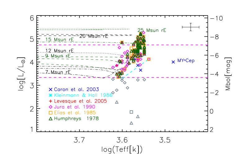
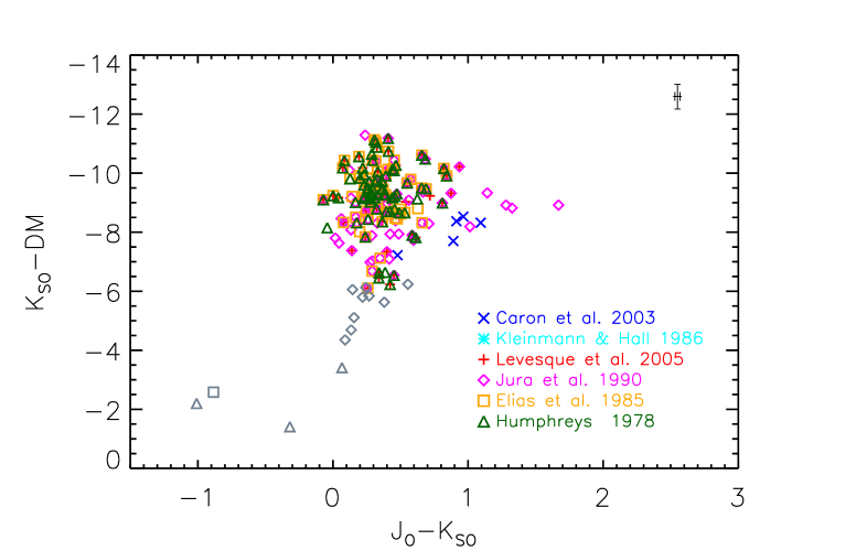
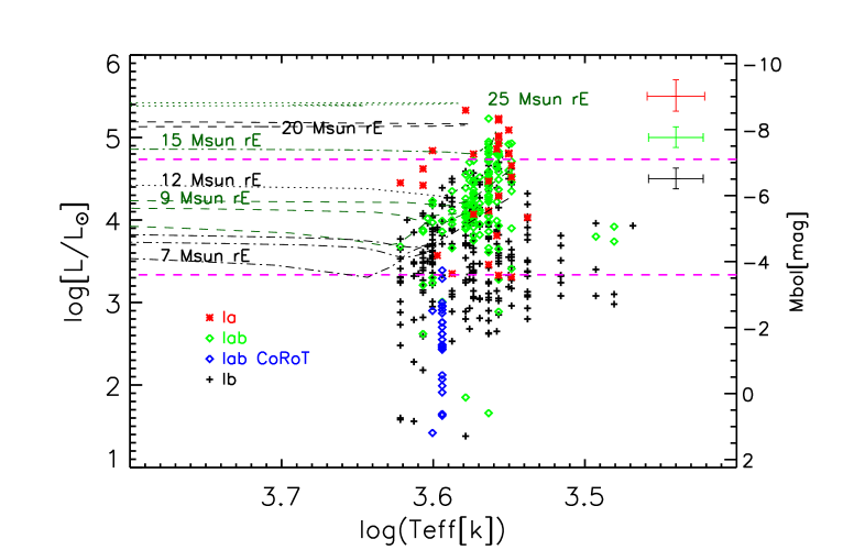
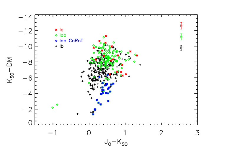
Figure 3.— Left-upper Panel: Luminosities versus T_eff values of reference RSGs (from class Ia to Ib), i.e. of the subsample of stars in Table 2 with given class I in the catalogs of Caron et al. (2003, blue crosses), Kleinmann & Hall (1986, cyan asterisck), Levesque et al. (2005, red pluses), (Jura & Kleinmann 1990, magenta diamonds), Elias et al. (1985, orange squares), and Humphreys (1978, green triangles). An average error bar is drawn on the right-upper corner. The two magenta long-dashed horizontal lines marks M_bol=$-3.6$ mag (tip of the red giant branch), and $-7.1$ mag (AGB limit). The long-dashed cyan line marks the Eq. (1); RSGs appear brighter and bluer than that locus (see text). Stellar tracks from models at solar metallicity and including rotation are from Ekström et al. (2012); from the bottom to the top: the black dotted-dashed curve marks a stellar track of a 7 M_⊙ star; the green long-dashed curve marks a 9 M_⊙ track; the black dotted curve a 12 M_⊙ track; the green dotted-dashed curve shows a 15 M_⊙ track; the black long-dashed the track of a 20 M_⊙ track, and the top green dotted line that of a 25 M_⊙. A few objects (in grey) remain fainter than the red giant tip (see text). Right-upper Panel: Absolute and dereddened K_s magnitudes versus de-reddened $J-$K_s colors. Data points are as described in the left panel. Right-lower Panel: Luminosities versus T_eff values of stars in Table 2 with adopted class Ia, Iab, and Ib (stars detected by CoRoT and listed in Table 2 as class Iab should be regarded separately). Left-lower Panel: Absolute and dereddened K_s magnitudes versus de-reddened $J-$K_s colors of stars in Table 2 with adopted class Ia, Iab, and Ib.

3.2.1 Reference RSGs

We consider as reference RSGs those stars included in the catalogs of Kleinmann & Hall (1986), Levesque et al. (2005), Caron et al. (2003), Jura & Kleinmann (1990), Elias et al. (1985), and Humphreys (1978). These sources are expected to be RSGs, because they are located in the direction of OB associations. In the upper-left panel of Fig. 3, we show their luminosities, $\log(L/$L_⊙), versus T_eff (theoretical plane); in the lower panel, we show their absolute and dereddened K_s, $K_{\rm so}-$DM versus $J_{\rm o}-K_{\rm so}$ (observational plane); DM is the distance moduli. By comparison with the stellar tracks, we estimated initial masses from about 7 to 25 M_⊙ (Ekström et al. 2012). Among them, the brighest star appears to be SW Cep with M_bol= $-8.42$ mag. MY-Cep is the only M7.5 I included in the sample. A few stars were discarded as reference RSGs, because they appeared too faint for luminosity class I (M_bol $>-3.6$ mag, as shown in Fig. 3); those stars are IRC+40105, 6 Aur, 1 Pup, sigOph, IRC +00328, 33 Sgr, 12 Peg, BD+47 3584, 56 Peg (Jura & Kleinmann 1990), CD-57 3502 (Elias et al. 1985), CPD-59 4549, HD 142686, and HD 150675 (Humphreys 1978).

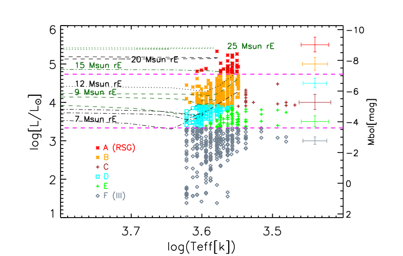
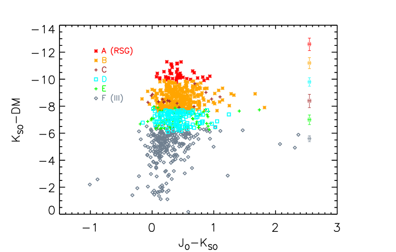
Figure 4.— Left Panel: Luminosities versus T_eff values of stars in Table 2 with $\varpi/{\sigma_{\varpi}}({\rm ext})>4$ and $\text{RUWE}<2.7$. Red asterisks mark highly-probable RSGs with M_bol$<-7.1$ mag (Area=A). Orange asterisks mark sources with M_bol$<-5.0$ mag and types $<M4$ (Area=B). Cyan squares mark sources with $-3.6>$M_bol$>-5.0$ mag and bluer that Eq. (1) (Area=D). Brown pluses (M_bol$<-5.0$ mag) and green pluses ($-3.6>$M_bol$>-5.0$ mag) indicate the Areas C and E. Gray diamonds indicate giants, i.e., stars fainter than M_bol$\approx-3.6$ mag (tip of the red giant branch, Area=F). The two magenta long-dashed horizontal lines mark M_bol=$-3.6$ mag (tip), mag, and M_bol=$-7.1$ mag (AGB limit). For comparison, we add some rotating stellar tracks with solar metallicity by Ekström et al. (2012). From the bottom to the top: the black dotted-dashed curve marks a stellar track of a 7 M_⊙ star; the green long-dashed curve marks a 9 M_⊙ track; the black dotted curve a 12 M_⊙ track; the green dotted-dashed curve shows a 15 M_⊙ track; the black long-dashed the track of a 20 M_⊙ track, and the top green dotted line that of a 25 M_⊙. Right Panel: Absolute and dereddened K_s magnitudes versus de-reddened $J-$K_s colors. Data points are as described in the left panel.

3.2.2 Hertzsprung-Russell diagram

All reference RSGs, but MY Cep, appear located along the ascending stellar tracks in Fig. 3. They are located to the left of the following equation (which is roughly parallel to the ascending parts of the tracks at the low T_eff end):

$$\log(L/\hbox{\it L${}_{\odot}$})=51.3-13.33\times\log(\hbox{\it T${}_{\rm eff}$})\,,$$ (1)

where $\log(\hbox{\it T${}_{\rm eff}$})$ ranges from 3.54 to 3.6 (i.e., from M4 to K1, Levesque et al. 2005).

The temporal evolution of an AGB star is characterised by large excursion in the M_bol versus T_eff diagram. During the thermal pulses the luminosity increases and T_eff decreases. For example, a star 3 M_⊙ may reach M_bol=$\approx-2$ mag during the early-AGB phase and M_bol=$\approx-5$ mag during thermal pulses (e.g., Vassiliadis & Wood (1993)).

In Fig. 4, we show the luminosities of stars in Table 6, and we verify their positions on the M_bol versus T_eff diagram by using the described observational benchmarks and the features appearing in Fig. 3:

• Area A contains late-type stars with M_bol$\lesssim-7.1$ mag, those are expected to be mostly RSGs.

• Area B contains stars with $-5.0>$M_bol$>-7.1$ mag and earlier than an M4. This area is rich in stars with masses larger than 7 M_⊙.

• Area C contains late-type stars with $-5.0>$M_bol$>-7.1$ mag and later than an M4. This area is expected to be dominated by AGBs (4-9 M_⊙).

• Area D contains late-type stars with $-3.6>$M_bol$>-5.0$ mag and bluer than Eq. (1). This area contain AGBs of intermediate masses and some faint K-type 9 M_⊙ stars at the onset of their cold phase (M_bol= $-4.5$ mag).

• Area E contains late-type stars with $-3.6>$M_bol$>-5.0$ mag and redder than Eq. (1). This area is expected to be dominated by old and more abundant AGBs (2-3 M_⊙).

• Area F contains late-type stars with M_bol$>-3.6$ mag. Those stars are fainter than the tip of the red giant branch.

In Fig. 4, in the theoretical M_bol versus T_eff diagram as well as in the observational $K_{\rm so}-$DM versus $J_{o}-K_{so}$ diagram, we mark the areas defined above with different colors. These luminosity areas are also added in Table 6. In Fig. 5, we show an histogram of the spectral types of the 889 sources with $\varpi/\sigma_{\varpi}>4$ and $\text{RUWE}<2.7$.

Reference RSGs appear to be made by stars with class Ia and Iab (35%), as well as of stars with class Ib (33%). In Figs. 3 and 5, the distribution of reference RSGs appears similar to that of stars Ia and Iab, with stars falling mostly in the Area A and B; but it’s different than that of class Ib stars, which are sparsely distributed over the Area A,B,C,E, and F.

From Table 2, about 43 sources (5%) are found to be located in the Area A (M_bol$\lesssim-7.1$ mag). Among them there are two stars, HD 99619 and HD 105563 A, with previous uncertain class. 312 sources (35%) are located in Area B and are likely more massive than 7 M_⊙. About 30% of the sample is made of stars fainter than the tip of the red giant branch (Area F).

A large number of RSGs detected at infrared wavelength (about 300) was included in the presented compilation; however for most of those stars parallaxes are not available in DR2 (Table 5 shows only 16 stars from infrared catalogs), (for example, Davies et al. 2008, 2007; Liermann et al. 2009; Clark et al. 2009; Negueruela et al. 2010, 2011, 2012; Messineo et al. 2017).

3.3. Gaia variables

We searched our sample for the presence of Gaia variables and found that only 137 stars of the initial 1342 source with Gaia data were flagged as variables (Holl et al. 2018), and 90 out of the 889 with good parallaxes (about 10%). The spectral types of all 90 but one variables range from K5 to M7, and 83 of them are automatically classified by the Gaia pipeline as long period variables, LPVs, including Mira and semiregular (SR) stars. Their average variation in $G$-band is 0.51 mag with a dispersion around the mean of 0.38 mag, including two stars with variations above 2.5 mag (0.1%), which are in Area C and E. There are 65 (out of 90) variables in Area A and B; their variations in $G$-band range from 0.2 mag to 0.8 mag, with a mean variation of 0.41 mag and dispersion around the mean of 0.14 mag. Similar values are found with the 9 variables of class Ib (a mean of 0.46 mag and a $\sigma=0.33$ mag). There are 9 variables fainter than M_bol$>-3.6$ mag (Area F), with 7 of them later than M5. Their mean variation is 0.63 mag and $\sigma=0.45$ mag.

An analysis of the $G$-band light curves will be presented elsewhere.

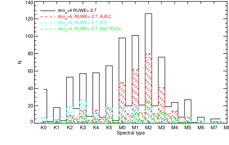
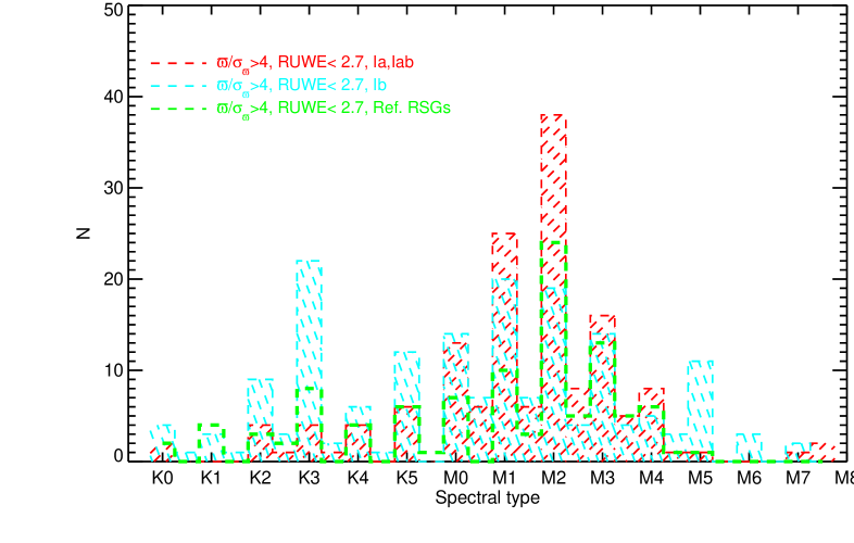
Figure 5.— Right panel: In black the histogram of the spectral types of sources with good distances ($\varpi/{\sigma_{\varpi}}({\rm ext})>4$ and $\text{RUWE}<2.7$); in red that of sources with M_bol$<-5.0$ mag, i.e located in Area A and B, or in Area C but reported with class I in all previous literature; in cyan the histogram of sources with M_bol$>-5.0$ mag, located in Area D, or in Area E but reported with class I in all previous literature; in green the histogram of reference RSGs. Right panel: in red sources of adopted class Ia, Iab and with good distances and M_bol$<-3.6$ mag; in cyan the histogram of sources of adopted class Ib with good distances and M_bol$<-3.6$ mag; in green the histogram of reference RSGs.

Table 5 Numbers of collected stars per luminosity classes.

Sample	N(sp)	N(Ks)	N(plx)	N(Ks+plx)
				NA	NB	ND	NCE	NF	Nnew(I)
					blue	blue	red	(III)
Alla	1406	1406	889	43	322	134	110	280	35
Ref. opt starsb	170	170	135	26	69	21	2	17	0
Ref. IR stars c	312	312	16	0	1	3	0	12	1
Nsp(Ia)	57	57	28	12	9	1	4	2	0
Nsp(Iab)	243	243	161	16	90	11	9	35	0
Nsp(Ib)	300	300	259	2	76	52	48	81	0
Nsp(any I)	1013	1013	620	41	253	86	82	158	0
Nsp(I-II)	166	166	113	0	36	24	14	39	0

• Notes. N(sp) = number of stars with known available spectral types.  N(Ks) = number of stars with available near-infrared measurements.  N(plx)= number of stars with $\varpi/{\sigma_{\varpi}}({\rm ext})>4$ and $\text{RUWE}<2.7$.  N_A= number of stars located in Area A.  N_B= number of stars located in Area B.  N_D= number of stars located in Area D.  N_CE= number of stars located in Area C or E.  N_F = number of stars in Area F.  Nnew(I)=number of stars without adopted classes and to which we assign Area A or B.

  Nsp(Ia) = number of stars with luminosity classes Ia.  Nsp(Iab) = number of stars with luminosity classes Iab.  Nsp(Ib) = number of stars with luminosity classes Ib.  Nsp(any I)= number of stars with luminosity classes (I,Ia,Iab,Ib).  Nsp(I-II) = number of stars with luminosity classes (I-II).  ($a$) All stars in Table 2.  ($b$) Example of optically visible RSGs taken from Caron et al. (2003), Levesque et al. (2005), Jura & Kleinmann (1990), Kleinmann & Hall (1986), Elias et al. (1985), and Humphreys (1978).  ($c$) Example of optically obscured sources taken from Messineo et al. (2017), Clark et al. (2009), Davies et al. (2008), Davies et al. (2007), Negueruela et al. (2012), Negueruela et al. (2011), Negueruela et al. (2010), and Liermann et al. (2009).

3.4. Average magnitudes per spectral type.

In Table 7 we present average magnitudes per spectral type of stars of class I and with M_bol$<-5.0$ mag, and of stars with $-3.6<$M_bol$<-5.0$ mag. This table is useful for Galactic star counts (e.g. Wainscoat et al. 1992). In Table 2 of Just et al. (2015) infrared luminosities of Hipparcos stars per classes are also provided; for example, their K-M2 I-II stars have M_K= $-9$ mag. For stars with spectral types K-M2 I and M_bol$<-5.0$ mag, our Table 7 provides an average M_K= $-8.40$ mag with $\sigma$=0.39 mag.

Additionally, in Tables 8 and 9 we present average magnitudes per spectral type of stars of classes Ia and Iab and of stars in the reference RSG sample.

In Fig. 7, we plot the calculated average magnitudes per spectral types of stars with classes Ia and Iab, as well as of stars in the reference RSG sample, versus the T_eff values. T_eff were estimated from the spectral types with the temperature scale given by Levesque et al. (2005). For stars with T_eff from 3650 k to 3950 k, M_bol values seem to decrease with decreasing T_eff values.

3.5. Spatial distribution

The bright cool stars here analyzed span 360^∘ of longitude (Fig. 6). By using the estimates of distances in Table 2, we obtained the distribution on the Galactic plane shown in Fig. 6. Late-type stars brighter than M_bol=$-5.0$ mag ($0.8\times 10^{4}$ L_⊙) appear radially more distant from the Sun than the whole sample, with heliocentric distances ranging from $\approx 200$ to $\approx 4600$ pc. Star eta Per (K3 Ib-II) is 239 pc away from us ($\varpi=4.21\pm 0.37$ mas), and HD 200905 (K4.5 I) is 283 pc away ($\varpi=3.59\pm 0.42$ mas). Antares (alpha Sco, M1.5 Iab) with an estimated distance of $\approx 170$ pc does not have Gaia parallax measurement yet. PER286 (M2.0 Ib) has an estimated distance of 4.2 kpc ($\varpi=0.20\pm 0.04$ mas).

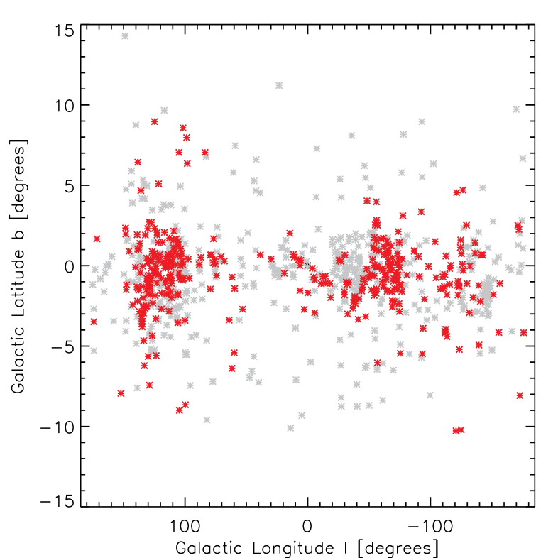
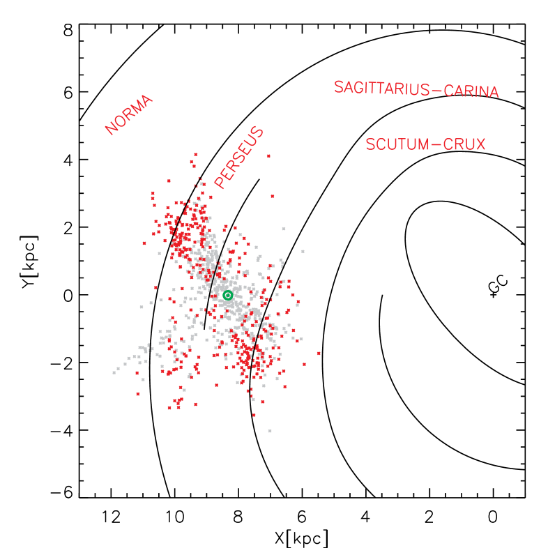
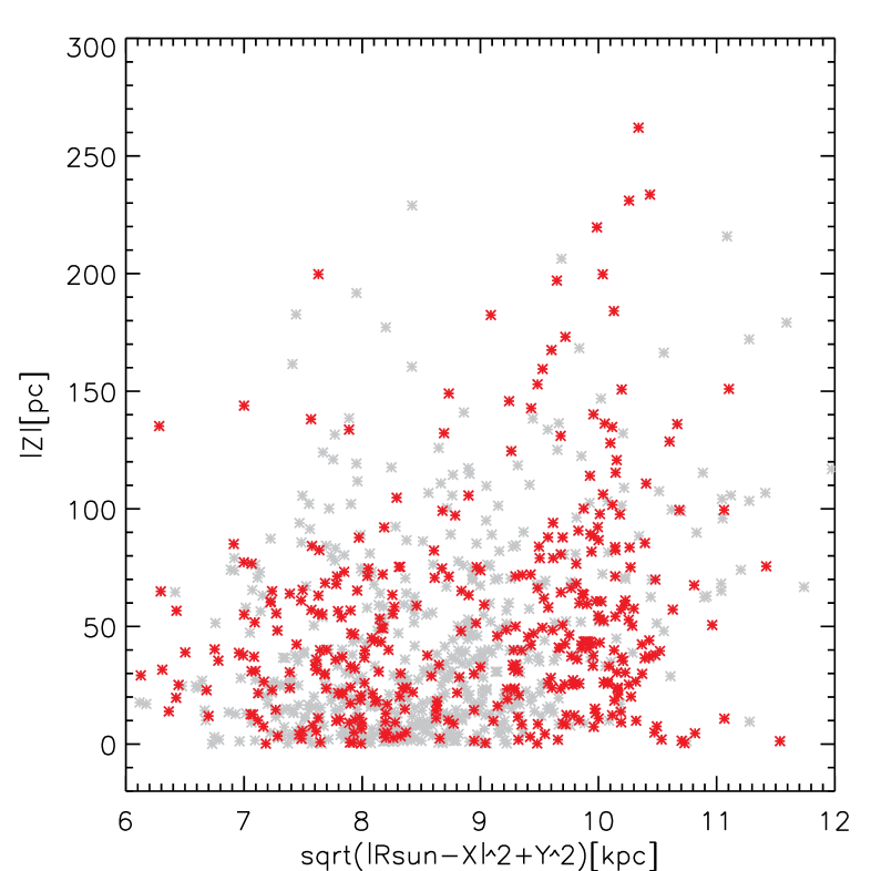
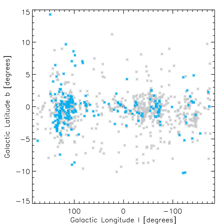
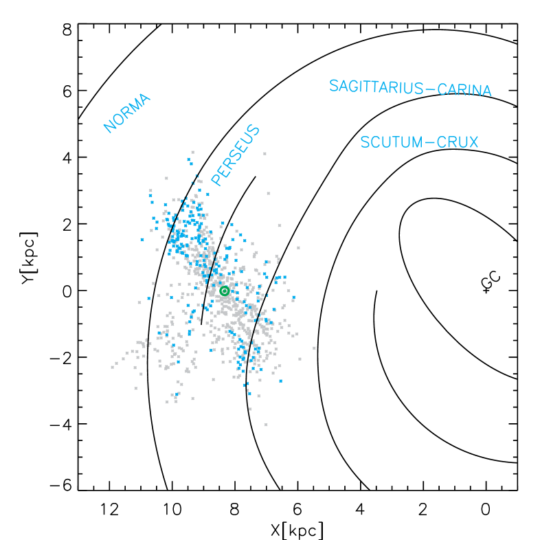
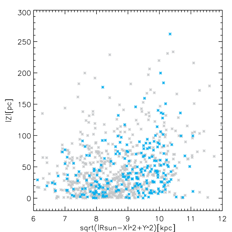
Figure 6.— Left-upper panel: Latitudes versus longitudes of the bright late-type stars in Table 2. Candidate RSGs with M_bol$<-5.0$ mag (Area A and B) and $\varpi/{\sigma_{\varpi}}({\rm ext})>4$ and $\text{RUWE}<2.7$ are marked in red. Central-upper panel: Galactocentric coordinates $XY$ on the disk of the Milky Way. The Sun location (8.5,0) is marked in green, while the Galactic Centre (GC) marked with a black cross is at (0,0). The spiral arms are taken from the work of Cordes & Lazio (2003). Right-upper panel: Distances from the plane $|Z|$ versus Galactocentric distances. Lower panels: As in the uppe panels, but this time cyan asterisks mark bright late-type stars in Table 2 with class Ia or Iab, or reference RSGs (see Fig. 3).

4. Summary

In order to create a catalog of stars with luminosity class I, candidate RSGs, from Gaia DR2, we collected 1406 bright late-type stars with at least one spectroscopic record as class I. Spectral types were taken from the collection by Skiff (2014), and in the majority of cases appeared within the uncertainty of 2 subclasses (i.e., the range of types reported for a single entry). For well known sources, such as those analyzed by Dorda et al. (2018), Dorda et al. (2016), Levesque et al. (2005), Jura & Kleinmann (1990), Elias et al. (1985), and Humphreys (1978), spectral types and luminosity classes were taken from these works. At the present time, only a fraction equal to 13% of this sample is known to be associated with open clusters. For each source, we collected available photometric measurements from 2MASS, CIO, MSX, WISE, MIPSGAL, GLIMPSE, and NOMAD catalogs and estimated their apparent bolometric magnitudes.

We retrieved parallaxes for 1342 sources from Gaia DR2, of which 1290 have a $(G_{\mathrm{BP}}-G_{\mathrm{RP}})$ colour. After a data filtering based on signal to noise and astrometric quality ($\varpi/\sigma_{\varpi}>4$ and $\text{RUWE}<2.7$), we were left with a best-quality sample of 889 sources.

With the parallactic distances, we were able to estimate the stellar luminosities, and to build M_bol versus T_eff diagrams of stars with different classes.

The Galactic catalog of RSGs, i.e., of very likely massive stars because of luminosity and associations with OB stars, by Humphreys (1978), Elias et al. (1985), Jura & Kleinmann (1990), Levesque et al. (2005), Caron et al. (2003) contains 170 stars. 118 of these reference RSGs had good parallaxes in DR2 and M_bol$<-3.6$ mag. While these reference RSGs appear to contain stars of class Ia, Iab (40%) as well as class Ib (31%), their distribution on the M_bol versus T_eff diagrams resembles that of class Ia, Iab, with 81% of them located in Area A and B. Only 44% of class Ib stars with M_bol$<-3.6$ mag fall in Area A and B.

For 609 stars (68% of 889 analysed stars), M_bol values were found smaller (brighter) than $-3.6$ mag, with 536 of them already reported in previous literature exclusively as of classes I or II. 5% of the them appear highly-probable massive stars (stars in Area A), while 41 % of them are stars in Area A and B, likely more massive than 7M_⊙.

A fraction equal to $\approx 30$% of the sample appears to be made of stars fainter than the tip of the giant branch (Area F).

A natural output of this luminosity exercise is a tabulated average of absolute magnitudes of luminous late-type stars and RSGs per spectral type. This finer grid of magnitudes will help to predict distances of extragalactic luminous late-type stars.

This catalog is a little exercise on the use of accumulate spectroscopic knowledge in support of the Gaia mission. The catalog serve for high-resolution follow-up spectroscopy, for example, with ongoing large spectroscopic surveys such as LAMOST and GALAH. This is important to understand the evolution and nucleosynthesis occurring in RSGs and massive AGBs (and super-AGB stars). Luminosities, spectral types, and chemistry are key ingredients for an improved study of the Galactic structure and its recent history.

Table 6 Properties of bright late-type stars from Table 2.

Id	Sp.Type	Class(adopt)	Area	Teff	J-Ks	H-Ks	A${}_{\rm K_{s}}$(JK)	A${}_{\rm K_{s}}$(HK)	BC${}_{K_{\rm s}}$a	Ksob	Mbolc	Mbol2d	DMe	Mbol-Qf	$V_{o}$	R
				[K]	[mag]	[mag]	[mag]	[mag]	[mag]	[mag]	[mag]	[mag]	[mag]		[mag]	[$R_{\odot}$]
1	M4.5	Ib	E	3535.00 $\pm$ 170.00	1.25	0.30	0.07 $\pm$ 0.19	0.24 $\pm$ 0.47	2.89	2.11 $\pm$ 0.31	$-$4.35 ${}^{-0.33}_{+0.32}$	$-$4.24 ${}^{-0.26}_{+0.25}$	9.36 ${}^{-0.10}_{+0.09}$	2	7.88	175
2	M3	Ib	F	3605.00 $\pm$ 170.00	1.16	0.28	0.03 $\pm$ 0.01	0.06 $\pm$ 0.03	2.84	4.27 $\pm$ 0.02	$-$2.87 ${}^{-0.10}_{+0.10}$	$-$2.76 ${}^{-0.09}_{+0.09}$	9.98 ${}^{-0.08}_{+0.08}$	2	9.45	85
3	M5	Ib	F	3450.00 $\pm$ 170.00	1.30	0.32	0.01 $\pm$ 0.01	0.09 $\pm$ 0.06	2.96	4.47 $\pm$ 0.02	$-$2.94 ${}^{-0.22}_{+0.20}$	$-$2.83 ${}^{-0.21}_{+0.20}$	10.36 ${}^{-0.21}_{+0.19}$	1	$..$	96
4	M2	Iab	A	3660.00 $\pm$ 170.00	1.06	0.25	0.22 $\pm$ 0.18	0.24 $\pm$ 0.48	2.80	1.51 $\pm$ 0.29	$-$7.55 ${}^{-0.47}_{+0.43}$	$-$7.54 ${}^{-0.42}_{+0.38}$	11.86 ${}^{-0.36}_{+0.31}$	2	6.39	716
5	M1	Ib	B	3745.00 $\pm$ 170.00	1.00	0.22	$-$0.02 $\pm$ 0.22	0.03 $\pm$ 0.70	2.73	4.29 $\pm$ 0.46	$-$5.42 ${}^{-0.59}_{+0.56}$	$-$5.35 ${}^{-0.39}_{+0.36}$	12.44 ${}^{-0.36}_{+0.32}$	2	9.57	256
6	K0	Iab	D	4185.00 $\pm$ 85.00	0.58	0.12	0.43 $\pm$ 0.15	0.46 $\pm$ 0.40	2.40	3.21 $\pm$ 0.15	$-$4.45 ${}^{-0.17}_{+0.17}$	$-$4.36 ${}^{-0.25}_{+0.25}$	10.06 ${}^{-0.06}_{+0.06}$	1	3.68	131
7	K3	Ib	F	3985.83 $\pm$ 170.00	0.72	0.15	0.24 $\pm$ 0.18	0.23 $\pm$ 0.44	2.55	3.11 $\pm$ 0.29	$-$2.63 ${}^{-0.30}_{+0.30}$	$-$2.58 ${}^{-0.23}_{+0.23}$	8.30 ${}^{-0.03}_{+0.03}$	2	6.02	62
8	M1	Iab	B	3745.00 $\pm$ 170.00	1.00	0.22	0.29 $\pm$ 0.21	0.40 $\pm$ 0.58	2.73	2.97 $\pm$ 0.37	$-$6.03 ${}^{-0.41}_{+0.41}$	$-$5.93 ${}^{-0.29}_{+0.29}$	11.73 ${}^{-0.16}_{+0.15}$	2	6.53	339
9	M1	Iab	B	3745.00 $\pm$ 170.00	1.00	0.22	0.13 $\pm$ 0.18	0.24 $\pm$ 0.43	2.73	1.75 $\pm$ 0.28	$-$5.91 ${}^{-0.36}_{+0.35}$	$-$5.82 ${}^{-0.31}_{+0.30}$	10.39 ${}^{-0.22}_{+0.20}$	2	5.70	321
10	M2	I	B	3660.00 $\pm$ 170.00	1.06	0.25	0.43 $\pm$ 0.23	0.70 $\pm$ 0.55	2.80	2.27 $\pm$ 0.37	$-$6.18 ${}^{-0.46}_{+0.44}$	$-$6.15 ${}^{-0.37}_{+0.36}$	11.26 ${}^{-0.26}_{+0.24}$	2	5.78	381

• Notes. The identification number (Id) from 2 is followed by the spectral type and class adopted from literature, Sp(adopt) and Class(adopt), by the area occupied in the M_bol vs. T_eff plot (Area), the T_eff value, the intrinsic J-K_s and H-K_s colors, the extinction A${}_{\rm K_{s}}$(JK) and A${}_{\rm K_{s}}$(HK) derived from the $JK$ and $HK$ colors, the adopted BC${}_{K_{\rm s}}$, the dereddened K_s, K_so, two estimates of bolometric magnitudes, the DM obtained with the distances of Bailer-Jones et al. (2018), a flag for best near-infrared photometry (Mbol-Q), the dereddened $V$ magnitude, $V_{o}$, and the stellar radius (R) estimated with the equation of Josselin & Plez (2007).
  A few A${}_{K_{\rm s}}$ values are negative. No extinction correction was applied for these stars.
  (^a) For BC_K, values are calculated with the formula of Levesque et al. (2005) and a typical error of 0.06 mag is assumed (average difference between the BC_K values of two spectral types).
  (^b) The errors on the K_so values are estimated by propagating the photometric errors and the A${}_{K_{\rm s}}$ errors.
  (^c) The M_bol values are obtained with the BC_K, their errors are estimated by propagating the errors on K_so, BC_K, and DMs.
  (^d) The M_bol2 values are obtained via integration under the SED (see Sect. 3.1). Errors are estimating by lowering the curve by subtracting the photometric errors, and by lifting up the curve by adding the photometric curve. The DM error is then added by Taylor’s propagation law. (^e) DM is here the distance module obtained with the Bailer distance. Its error is obtained using the quoted high and low values Bailer-Jones et al. (2018).
  (^f) Mbol-Q is set to unity when $\varpi/\sigma_{\varpi}>4$ and $\text{RUWE}<2.7$ (889 sources), set to 2 when $\varpi/\sigma_{\varpi}>4$ and $\text{RUWE}<2.7$ and $JH$K_s  quality flags are $A$ (2MASS) or $B$ (2MASS) or $C$ (2MASS) or $D$ (2MASS) or $M$ (HST photometry) (see Appendix).

Table 7 Magnitudes per spectral types

Nstar	Sp.Type	Mbol	MK	${\rm M_{V}}$	Mbol-bin	$V-K^{a}$
		[mag]	[mag]	[mag]	[mag]
3	K0.5-K0	$-$5.71$\pm$ 0.34	$-$8.12$\pm$ 0.33	$-$6.86$\pm$ 1.01	$<-$5.	2.16
2	K1.5-K1	$-$6.04$\pm$ 0.22	$-$8.50$\pm$ 0.22	$-$6.77$\pm$ 0.27	$<-$5.	2.29
15	K2.5-K2	$-$5.74$\pm$ 0.17	$-$8.25$\pm$ 0.17	$-$5.97$\pm$ 0.24	$<-$5.	2.44
18	K3.5-K3	$-$5.60$\pm$ 0.13	$-$8.15$\pm$ 0.13	$-$5.37$\pm$ 0.13	$<-$5.	2.72
20	K4.5-K4	$-$5.75$\pm$ 0.14	$-$8.35$\pm$ 0.14	$-$5.00$\pm$ 0.27	$<-$5.	3.00
21	K5.5-K5	$-$5.60$\pm$ 0.11	$-$8.24$\pm$ 0.11	$-$4.63$\pm$ 0.18	$<-$5.	3.70
60	M0.5-M0	$-$5.72$\pm$ 0.08	$-$8.42$\pm$ 0.08	$-$4.31$\pm$ 0.12	$<-$5.	3.79
74	M1.5-M1	$-$6.02$\pm$ 0.08	$-$8.76$\pm$ 0.08	$-$4.44$\pm$ 0.13	$<-$5.	3.92
91	M2.5-M2	$-$6.29$\pm$ 0.08	$-$9.09$\pm$ 0.08	$-$4.50$\pm$ 0.11	$<-$5.	4.11
52	M3.5-M3	$-$6.62$\pm$ 0.13	$-$9.47$\pm$ 0.13	$-$4.03$\pm$ 0.15	$<-$5.	4.58
15	M4.5-M4	$-$6.40$\pm$ 0.16	$-$9.29$\pm$ 0.16	$-$3.58$\pm$ 0.32	$<-$5.	5.24
7	M5.5-M5	$-$5.47$\pm$ 0.13	$-$8.43$\pm$ 0.13	$-$1.90$\pm$ 0.26	$<-$5.	6.06
3	M6.5-M6	$-$4.43$\pm$ 0.21	$-$7.52$\pm$ 0.22	0.56$\pm$ 0.93	[-3.6,-5.0]
7	M5.5-M5	$-$4.14$\pm$ 0.16	$-$7.10$\pm$ 0.16	0.14$\pm$ 0.35	[-3.6,-5.0]
7	M4.5-M4	$-$4.12$\pm$ 0.10	$-$7.01$\pm$ 0.10	$-$0.95$\pm$ 0.16	[-3.6,-5.0]
13	M3.5-M3	$-$4.39$\pm$ 0.09	$-$7.23$\pm$ 0.09	$-$0.94$\pm$ 0.57	[-3.6,-5.0]
23	M2.5-M2	$-$4.55$\pm$ 0.07	$-$7.36$\pm$ 0.07	$-$2.10$\pm$ 0.25	[-3.6,-5.0]
19	M1.5-M1	$-$4.28$\pm$ 0.10	$-$7.01$\pm$ 0.10	$-$2.39$\pm$ 0.17	[-3.6,-5.0]
21	M0.5-M0	$-$4.43$\pm$ 0.10	$-$7.13$\pm$ 0.09	$-$2.99$\pm$ 0.17	[-3.6,-5.0]
17	K5.5-K5	$-$4.54$\pm$ 0.10	$-$7.18$\pm$ 0.10	$-$2.79$\pm$ 0.25	[-3.6,-5.0]
14	K4.5-K4	$-$4.57$\pm$ 0.10	$-$7.17$\pm$ 0.10	$-$3.93$\pm$ 0.27	[-3.6,-5.0]
31	K3.5-K3	$-$4.34$\pm$ 0.06	$-$6.90$\pm$ 0.07	$-$3.85$\pm$ 0.11	[-3.6,-5.0]
27	K2.5-K2	$-$4.29$\pm$ 0.07	$-$6.80$\pm$ 0.07	$-$4.09$\pm$ 0.10	[-3.6,-5.0]
5	K1.5-K1	$-$4.16$\pm$ 0.22	$-$6.63$\pm$ 0.21	$-$4.37$\pm$ 0.24	[-3.6,-5.0]
8	K0.5-K0	$-$4.19$\pm$ 0.10	$-$6.59$\pm$ 0.10	$-$4.35$\pm$ 0.33	[-3.6,-5.0]

• Notes. Average magnitudes of stars in Table 6 with $\varpi/\sigma_{\varpi}>4$ and $\text{RUWE}<2.7$. The errors on the mean values are calculated as $\sqrt{\frac{\sum_{j=0}^{j=N-1}(\hbox{\it M${}_{\rm bol}$}_{j}-mean)^{2}}{N-1})\times\frac{1}{N}.}$ At the top, sources with M_bol$<-5.0$ mag and Area A or B, or Area C but with secure class I from previous literature. At the bottom, stars with $-3.6<$ M_bol$<-5.0$ mag and Area D, or E (but with secure class I from previous literature). (a) $V-K$ colours from Johnson (1966). Our $V-$K_s colours per spectral type are consistent within errors with the $V-K$ colours listed in the review by Johnson (1966) with a mean difference of $0.26$ mag and a dispersion around the mean of $0.28$ mag.

Table 8 Magnitudes per spectral types of stars with class Ia and Iab

Nstar	Sp.Type	Mbol	MK	${\rm M_{V}}$	Mbol-bin
		[mag]	[mag]	[mag]	[mag]
2	K0.5-K0	$-$5.41$\pm$ 0.97	$-$7.82$\pm$ 0.96	$-$6.11$\pm$ 0.27	$<-3.6$
5	K2.5-K2	$-$5.67$\pm$ 0.38	$-$8.18$\pm$ 0.38	$-$5.86$\pm$ 0.56	$<-3.6$
5	K3.5-K3	$-$5.66$\pm$ 0.52	$-$8.22$\pm$ 0.51	$-$5.13$\pm$ 0.56	$<-3.6$
3	K4.5-K4	$-$5.01$\pm$ 0.11	$-$7.61$\pm$ 0.11	$-$3.85$\pm$ 0.14	$<-3.6$
6	K5.5-K5	$-$5.02$\pm$ 0.36	$-$7.65$\pm$ 0.36	$-$3.66$\pm$ 0.78	$<-3.6$
19	M0.5-M0	$-$5.94$\pm$ 0.20	$-$8.64$\pm$ 0.20	$-$4.51$\pm$ 0.21	$<-3.6$
31	M1.5-M1	$-$5.80$\pm$ 0.11	$-$8.54$\pm$ 0.11	$-$4.09$\pm$ 0.22	$<-3.6$
46	M2.5-M2	$-$6.35$\pm$ 0.14	$-$9.15$\pm$ 0.14	$-$4.58$\pm$ 0.23	$<-3.6$
21	M3.5-M3	$-$7.05$\pm$ 0.22	$-$9.90$\pm$ 0.22	$-$4.06$\pm$ 0.31	$<-3.6$
9	M4.5-M4	$-$6.22$\pm$ 0.39	$-$9.11$\pm$ 0.38	$-$3.49$\pm$ 0.53	$<-3.6$
1	M5.5-M5	$-$5.33	$-$8.29	$-$2.49	$<-3.6$

• Notes. Average magnitudes of stars in Table 6 with $\varpi/\sigma_{\varpi}>4$ and $\text{RUWE}<2.7$ and class Ia and Iab.

Table 9 Magnitudes per spectral types of reference RSGs

Nstar	Sp.Type	Mbol	MK	${\rm M_{V}}$	Mbol-bin
		[mag]	[mag]	[mag]	[mag]
1	K0.5-K0	$-$4.68$\pm$ 0.30	$-$7.09$\pm$ 0.28	$-$4.77	$<-3.6$
2	K1.5-K1	$-$4.43$\pm$ 0.45	$-$6.89$\pm$ 0.44	$-$4.67$\pm$ 0.33	$<-3.6$
7	K2.5-K2	$-$4.37$\pm$ 0.26	$-$6.88$\pm$ 0.26	$-$4.51$\pm$ 0.28	$<-3.6$
10	K3.5-K3	$-$5.14$\pm$ 0.33	$-$7.69$\pm$ 0.33	$-$4.95$\pm$ 0.26	$<-3.6$
3	K4.5-K4	$-$4.92$\pm$ 0.46	$-$7.51$\pm$ 0.46	$-$4.80$\pm$ 0.55	$<-3.6$
7	K5.5-K5	$-$5.33$\pm$ 0.28	$-$7.97$\pm$ 0.28	$-$4.47$\pm$ 0.35	$<-3.6$
7	M0.5-M0	$-$5.99$\pm$ 0.16	$-$8.69$\pm$ 0.16	$-$4.80$\pm$ 0.20	$<-3.6$
15	M1.5-M1	$-$6.31$\pm$ 0.15	$-$9.05$\pm$ 0.15	$-$5.00$\pm$ 0.20	$<-3.6$
32	M2.5-M2	$-$6.54$\pm$ 0.12	$-$9.34$\pm$ 0.12	$-$4.78$\pm$ 0.15	$<-3.6$
22	M3.5-M3	$-$7.19$\pm$ 0.20	$-$10.04$\pm$ 0.20	$-$4.19$\pm$ 0.24	$<-3.6$
6	M4.5-M4	$-$6.57$\pm$ 0.14	$-$9.46$\pm$ 0.14	$-$3.43$\pm$ 0.25	$<-3.6$
1	M5.5-M5	$-$5.55$\pm$ 0.49	$-$8.51$\pm$ 0.35	$-$2.19	$<-3.6$

• Notes. Average magnitudes of stars plotted in the upper panels of Fig. 3.

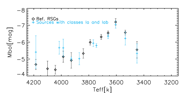
Figure 7.— Average M_bol versus T_eff. Cyan crosses show the values for class Ia and Iab stars. Black diamonds indicate the values for the reference RSGs.

Appendix A A. Notes on photometric data

Typically, initial coordinates by Skiff (2014) are good to within a few arcseconds. A few coordinates were corrected with SIMBAD. An iterative process was needed to make sure to properly identify the counterparts at different wavelengths. The Galactic plane is crowded with sources.

For stars at longitude $|l|>1$^∘ and latitude $|l|>0.5$^∘, measurements were associated automatically with a selection of good flags to ensure quality. MSX upper limits measurements were discarded, and WISE sources were chosen with a minimum signal-to-noise larger than 2. GLIMPSE matches were associated with a magnitude cut at 10 mag, and when a WISE source was existing positional coincidence was inspected. The searched stars were usually the brightest at near- and mid-infrared wavelengths, and chart identification was easy. 2MASS matches are as in the WISE and GLIMPSE catalogs. Due to saturation and centroid problems, a few 2MASS identifications had to be fixed (e.g. BD+54 315, VY CMa, Cl* Westerlund 1 26, MZM29, MZM33, RSGC1-F08, IRAS 17433$-$1750). For stars HD 126152, HD 149812, HD 227793, BD +36 4025, which have good quality parallaxes but no 2MASS errors, we assumed an error in K_s=0.8 mag (see the quality flag provided in Table 6). For omi02 Cyg, $JK$ photometry was taken from Morel & Magnenat (1978). For stars $[$MMF2014$]$ 78, $[$MFD2010$]$ 5, $[$GLIMPSE9$]$-6, and $[$MMF2014$]$ 46/$[$MFD2010$]$ 8, HST $HK$ data were available (Messineo et al. 2010); for the faint OGLE BW3 V 93508, near-infrared magnitudes are from Lucas et al. (2008). For the highly-crowded central region ($|l|<1.0$^∘and $|b|<0.5$^∘), only the $K$-band photometry of Liermann et al. (2009) is provided, and for stars IRC$-$30320 , IRC$-$30322, $[$RHI84$]$ 10$-$565, MZM115 the 2MASS photometry. For LHO036, which as a parallax, additional $JH$ measurements taken from the work of Stolte et al. (2015).

Matches were confirmed with a visual inspection of 2MASS and WISE images, as well as of their SEDs. After the visual inspection, a few measurements were discarded as of poor quality (e.g., confused, highly saturated, or strong background emission) and not compatible with the SED. For stars $[$MMF2014$]$ 46, GLIMPSE9-6, RSGC2-8, RSGC2-14, 2MASS J18451760-0343051, and 2MASS J18451722-0343136, MSX matches were removed. For stars Cl* Westerlund 1 20, Cl* Westerlund 1 75, $[$MMF2014$]$ 46, GLIMPSE9-6, RSGC1-F08, RSGC1-F05, and RSGC1-F01, WISE matches were removed because they are blended with other sources. For stars $[$HSD93b$]$ 48, $[$MNG2014$]$ vdB-H 222 778, $[$MNG2014$]$ vdB-H 222 664, $[$MNG2014$]$ vdB-H 222 479, $[$MMF2014$]$ 78, 2MASS J18410261$-$0552582, HD 195214, and 2MASS J18392955$-$0544222 only $W4$ measurements were removed because sources were too faint or confused at this longer wavelength. For stars 2MASS J17361839-2217306, RSGC1-F07, RSGC1-F10, RSGC1-F03, 2MASS J18395282-0535172, both $W3$ and $W4$ magnitudes were discarded. For HD 14580 and Cl* Westerlund 1 26, $W1$ and $W2$ magnitudes did not fit their SED.

References

- Alard et al. (2001) Alard, C., Blommaert, J. A. D. L., Cesarsky, C., et al. 2001, ApJ, 552, 289
- Alonso-Santiago et al. (2017) Alonso-Santiago, J., Negueruela, I., Marco, A., et al. 2017, MNRAS, 469, 1330
- Asaki et al. (2010) Asaki, Y., Deguchi, S., Imai, H., et al. 2010, ApJ, 721, 267
- Bailer-Jones (2015) Bailer-Jones, C. A. L. 2015, PASP, 127, 994
- Bailer-Jones et al. (2018) Bailer-Jones, C. A. L., Rybizki, J., Fouesneau, M., Mantelet, G., & Andrae, R. 2018, AJ, 156, 58
- Benjamin et al. (2005) Benjamin, R. A., Churchwell, E., Babler, B. L., et al. 2005, ApJ, 630, L149
- Blanco et al. (1984) Blanco, V. M., McCarthy, M. F., & Blanco, B. M. 1984, AJ, 89, 636
- Blum et al. (2003) Blum, R. D., Ramírez, S. V., Sellgren, K., & Olsen, K. 2003, ApJ, 597, 323
- Brogaard et al. (2017) Brogaard, K., VandenBerg, D. A., Bedin, L. R., et al. 2017, MNRAS, 468, 645
- Cambrésy et al. (2011) Cambrésy, L., Genova, F., Wenger, M., et al. 2011, in EAS Publications Series, Vol. 49, EAS Publications Series, ed. C. Sterken, 135–157
- Caron et al. (2003) Caron, G., Moffat, A. F. J., St-Louis, N., Wade, G. A., & Lester, J. B. 2003, AJ, 126, 1415
- Chen et al. (2007) Chen, X., Shen, Z.-Q., & Xu, Y. 2007, ChJAA, 7, 531
- Chiavassa et al. (2011) Chiavassa, A., Pasquato, E., Jorissen, A., et al. 2011, A&A, 528, A120
- Chieffi & Limongi (2013) Chieffi, A. & Limongi, M. 2013, ApJ, 764, 21
- Choi et al. (2008) Choi, Y. K., Hirota, T., Honma, M., et al. 2008, PASJ, 60, 1007
- Churchwell et al. (2009) Churchwell, E., Babler, B. L., Meade, M. R., et al. 2009, PASP, 121, 213
- Clark et al. (2009) Clark, J. S., Negueruela, I., Davies, B., et al. 2009, A&A, 498, 109
- Comerón et al. (2004) Comerón, F., Torra, J., Chiappini, C., et al. 2004, A&A, 425, 489
- Cordes & Lazio (2003) Cordes, J. M. & Lazio, T. J. W. 2003, ArXiv: astro-ph/0301598
- Cordier et al. (2007) Cordier, D., Pietrinferni, A., Cassisi, S., & Salaris, M. 2007, AJ, 133, 468
- Cutri et al. (2003) Cutri, R. M., Skrutskie, M. F., van Dyk, S., et al. 2003, 2MASS All Sky Catalog of point sources.
- Davidson et al. (2018) Davidson, K., Helmel, G., & Humphreys, R. M. 2018, Research Notes of the American Astronomical Society, 2, 133
- Davies et al. (2007) Davies, B., Figer, D. F., Kudritzki, R.-P., et al. 2007, ApJ, 671, 781
- Davies et al. (2008) Davies, B., Figer, D. F., Law, C. J., et al. 2008, ApJ, 676, 1016
- Davies et al. (2009) Davies, B., Origlia, L., Kudritzki, R.-P., et al. 2009, ApJ, 696, 2014
- Doherty et al. (2015) Doherty, C. L., Gil-Pons, P., Siess, L., Lattanzio, J. C., & Lau, H. H. B. 2015, MNRAS, 446, 2599
- Dorda et al. (2016) Dorda, R., González-Fernández, C., & Negueruela, I. 2016, A&A, 595, A105
- Dorda et al. (2018) Dorda, R., Negueruela, I., & González-Fernández, C. 2018, MNRAS, 475, 2003
- Egan et al. (2003) Egan, M. P., Price, S. D., Kraemer, K. E., et al. 2003, VizieR Online Data Catalog, 5114
- Eggenberger et al. (2002) Eggenberger, P., Meynet, G., & Maeder, A. 2002, A&A, 386, 576
- Ekström et al. (2012) Ekström, S., Georgy, C., Eggenberger, P., et al. 2012, A&A, 537, A146
- Elias et al. (1985) Elias, J. H., Frogel, J. A., & Humphreys, R. M. 1985, ApJS, 57, 91
- ESA (1997) ESA, ed. 1997, ESA Special Publication, Vol. 1200, The HIPPARCOS and TYCHO catalogues. Astrometric and photometric star catalogues derived from the ESA HIPPARCOS Space Astrometry Mission
- Ferraro et al. (2000) Ferraro, F. R., Montegriffo, P., Origlia, L., & Fusi Pecci, F. 2000, AJ, 119, 1282
- Figer et al. (2006) Figer, D. F., MacKenty, J. W., Robberto, M., et al. 2006, ApJ, 643, 1166
- Gaia Collaboration et al. (2018) Gaia Collaboration, Brown, A. G. A., Vallenari, A., et al. 2018, A&A, 616, A1
- Gaia Collaboration et al. (2016) Gaia Collaboration, Prusti, T., de Bruijne, J. H. J., et al. 2016, A&A, 595, A1
- Gehrz (1989) Gehrz, R. 1989, in IAU Symposium, Vol. 135, Interstellar Dust, ed. L. J. Allamandola & A. G. G. M. Tielens, 445
- Gezari et al. (1996) Gezari, D. Y., Pitts, P. S., Schmitz, M., & Mead, J. M. 1996, VizieR Online Data Catalog, 2209
- Glass & Feast (1973) Glass, I. S. & Feast, M. W. 1973, MNRAS, 163, 245
- Gray & Corbally (2009) Gray, R. O. & Corbally, J., C. 2009, Book: Stellar Spectral Classification, Princeton University Press
- Gutermuth & Heyer (2015) Gutermuth, R. A. & Heyer, M. 2015, AJ, 149, 64
- Holl et al. (2018) Holl, B., Audard, M., Nienartowicz, K., et al. 2018, A&A, 618, A30
- Humphreys (1978) Humphreys, R. M. 1978, ApJS, 38, 309
- Iben (1974) Iben, Jr., I. 1974, ARA&A, 12, 215
- Johnson (1966) Johnson, H. L. 1966, ARA&A, 4, 193
- Josselin & Plez (2007) Josselin, E. & Plez, B. 2007, A&A, 469, 671
- Jura & Kleinmann (1990) Jura, M. & Kleinmann, S. G. 1990, ApJS, 73, 769
- Just et al. (2015) Just, A., Fuchs, B., Jahreiß, H., et al. 2015, MNRAS, 451, 149
- Kleinmann & Hall (1986) Kleinmann, S. G. & Hall, D. N. B. 1986, ApJS, 62, 501
- Koornneef (1983) Koornneef, J. 1983, A&A, 128, 84
- Kusuno et al. (2013) Kusuno, K., Asaki, Y., Imai, H., & Oyama, T. 2013, ApJ, 774, 107
- Levesque et al. (2005) Levesque, E. M., Massey, P., Olsen, K. A. G., et al. 2005, ApJ, 628, 973
- Liermann et al. (2009) Liermann, A., Hamann, W.-R., & Oskinova, L. M. 2009, A&A, 494, 1137
- Lindegren et al. (2018) Lindegren, L., Hernández, J., Bombrun, A., et al. 2018, A&A, 616, A2
- Lucas et al. (2008) Lucas, P. W., Hoare, M. G., Longmore, A., et al. 2008, MNRAS, 391, 136
- Luri et al. (2018) Luri, X., Brown, A. G. A., Sarro, L. M., et al. 2018, A&A, 616, A9
- Massey et al. (2001) Massey, P., DeGioia-Eastwood, K., & Waterhouse, E. 2001, AJ, 121, 1050
- Mengel & Tacconi-Garman (2007) Mengel, S. & Tacconi-Garman, L. E. 2007, A&A, 466, 151
- Mermilliod et al. (2008) Mermilliod, J. C., Mayor, M., & Udry, S. 2008, A&A, 485, 303
- Messineo et al. (2010) Messineo, M., Figer, D. F., Davies, B., et al. 2010, ApJ, 708, 1241
- Messineo et al. (2008) Messineo, M., Figer, D. F., Davies, B., et al. 2008, ApJ, 683, L155
- Messineo et al. (2005) Messineo, M., Habing, H. J., Menten, K. M., et al. 2005, A&A, 435, 575
- Messineo et al. (2014) Messineo, M., Zhu, Q., Ivanov, V. D., et al. 2014, A&A, 571, A43
- Messineo et al. (2016) Messineo, M., Zhu, Q., Menten, K. M., et al. 2016, ApJ, 822, L5
- Messineo et al. (2017) Messineo, M., Zhu, Q., Menten, K. M., et al. 2017, ApJ, 836, 65
- Montegriffo et al. (1998) Montegriffo, P., Ferraro, F. R., Origlia, L., & Fusi Pecci, F. 1998, MNRAS, 297, 872
- Moravveji et al. (2013) Moravveji, E., Guinan, E. F., Khosroshahi, H., & Wasatonic, R. 2013, AJ, 146, 148
- Morel & Magnenat (1978) Morel, M. & Magnenat, P. 1978, A&AS, 34, 477
- Morgan et al. (1943) Morgan, W. W., Keenan, P. C., & Kellman, E. 1943, Book: An atlas of stellar spectra, with an outline of spectral classification, The University of Chicago press
- Negueruela et al. (2011) Negueruela, I., González-Fernández, C., Marco, A., & Clark, J. S. 2011, A&A, 528, A59
- Negueruela et al. (2010) Negueruela, I., González-Fernández, C., Marco, A., Clark, J. S., & Martínez-Núñez, S. 2010, A&A, 513, A74
- Negueruela et al. (2012) Negueruela, I., Marco, A., González-Fernández, C., et al. 2012, A&A, 547, A15
- Pasquato et al. (2011) Pasquato, E., Pourbaix, D., & Jorissen, A. 2011, A&A, 532, A13
- Price et al. (2001) Price, S. D., Egan, M. P., Carey, S. J., Mizuno, D. R., & Kuchar, T. A. 2001, AJ, 121, 2819
- Rayner et al. (2009) Rayner, J. T., Cushing, M. C., & Vacca, W. D. 2009, ApJS, 185, 289
- Skiff (2014) Skiff, B. A. 2014, VizieR Online Data Catalog, 1
- Skrutskie et al. (2006) Skrutskie, M. F., Cutri, R. M., Stiening, R., et al. 2006, AJ, 131, 1163
- Stolte et al. (2015) Stolte, A., Hußmann, B., Olczak, C., et al. 2015, A&A, 578, A4
- Sweigart et al. (1990) Sweigart, A. V., Greggio, L., & Renzini, A. 1990, ApJ, 364, 527
- Vassiliadis & Wood (1993) Vassiliadis, E. & Wood, P. R. 1993, ApJ, 413, 641
- Verheyen et al. (2012) Verheyen, L., Messineo, M., & Menten, K. M. 2012, A&A, 541, A36
- Verhoelst et al. (2009) Verhoelst, T., van der Zypen, N., Hony, S., et al. 2009, A&A, 498, 127
- Wainscoat et al. (1992) Wainscoat, R. J., Cohen, M., Volk, K., Walker, H. J., & Schwartz, D. E. 1992, ApJS, 83, 111
- Wright et al. (2010) Wright, E. L., Eisenhardt, P. R. M., Mainzer, A. K., et al. 2010, AJ, 140, 1868
- Xu et al. (2018) Xu, S., Zhang, B., Reid, M. J., et al. 2018, ApJ, 859, 14
- Zacharias et al. (2005) Zacharias, N., Monet, D. G., Levine, S. E., et al. 2005, VizieR Online Data Catalog, 1297
- Zhang et al. (2012) Zhang, B., Reid, M. J., Menten, K. M., & Zheng, X. W. 2012, ApJ, 744, 23