Supervised Online Hashing via Hadamard Codebook Learning

Abstract.

In recent years, binary code learning, a.k.a. hashing, has received extensive attention in large-scale multimedia retrieval. It aims to encode high-dimensional data points into binary codes, hence the original high-dimensional metric space can be efficiently approximated via Hamming space. However, most existing hashing methods adopted offline batch learning, which is not suitable to handle incremental datasets with streaming data or new instances. In contrast, the robustness of the existing online hashing remains as an open problem, while the embedding of supervised/semantic information hardly boosts the performance of the online hashing, mainly due to the defect of unknown category numbers in supervised learning. In this paper, we propose an online hashing scheme, termed Hadamard Codebook based Online Hashing (HCOH), which aims to solve the above problems towards robust and supervised online hashing. In particular, we first assign an appropriate high-dimensional binary codes to each class label, which is generated randomly by Hadamard codes. Subsequently, LSH is adopted to reduce the length of such Hadamard codes in accordance with the hash bits, which can adapt the predefined binary codes online, and theoretically guarantee the semantic similarity. Finally, we consider the setting of stochastic data acquisition, which facilitates our method to efficiently learn the corresponding hashing functions via stochastic gradient descend (SGD) online. Notably, the proposed HCOH can be embedded with supervised labels and is not limited to a predefined category number. Extensive experiments on three widely-used benchmarks demonstrate the merits of the proposed scheme over the state-of-the-art methods. The code is available at https://github.com/lmbxmu/mycode/tree/master/2018ACMMM_HCOH.

ACM Reference Format:
Mingbao Lin, Rongrong Ji, Hong Liu, Yongjian Wu. 2018. Supervised Online Hashing via Hadamard Codebook Learning. In 2018 ACM Multimedia Conference (MM ’18), October 22-26, 2018, Seoul, Republic of Korea. ACM, New York, NY, USA, 9 pages. https://doi.org/10.1145/3240508.3240519

1. Introduction

With the growth of data scales, hashing-based methods have attracted extensive research attentions in large-scale multimedia retrieval (Wang et al., 2018), which merits in low storage and efficient computation on large-scale datasets. In principle, most existing works aim to map high-dimensional data into a compact Hamming space, such that the original data similarity can be approximated via Hamming distance efficiently. To this end, most effective hashing schemes are “data dependent”, which relies on modeling labeled or unlabeled data to learn discriminative binary codes (Weiss et al., 2009; Gong et al., 2013; Heo et al., 2012; Liu et al., 2014, 2017, 2012; Shen et al., 2015; Lu et al., 2017).

However, such a setting is hardly workable for various real-world applications. Many applications require the search engine ​ to index streaming data online. In contrast, most existing works in hashing adopt batch-based learning on the prepared training data, which is only suitable for fixed dataset. While facing new data, batch-based learning ​ has to accumulate all the available data and re-learns​ all hash functions. To handle this problem, advanced batch-based hashing (Liu et al., 2017; Jiang and Li, 2018) has been proposed to perform multiple passes over the data. ​ Unfortunately, the frequent data loading becomes a major performance bottleneck. In order to address the above challenges, online hashing (OH) (Shalev-Shwartz et al., 2012; Wang et al., 2014; Crammer et al., 2004) has been proposed to perform online learning of hash functions in an efficient way. However, two open problems still exist:

Firstly, most OH methods require that the input data should be fed with pairs or batches (Leng et al., 2015; Huang et al., 2013; Cakir et al., 2017b), while little works consider the case of a single datum input. To tackle this problem, inspired by the Error Correcting Output Codes (ECOCs), Cakir et al. proposed an online supervised hashing to solve such an extreme input (Cakir et al., 2017a), which uses an SGD of the supervised hashing with error correcting codes. But, the random construction for error correcting code will corrupt the model, which degenerates the retrieval performance.

Secondly, the unsupervised OH method (Leng et al., 2015) can not make full use of the label information and suffers from low performance, which has to adopt a batch of training data to update the hash functions. ​ Meanwhile, the performance of the existing supervised OH schemes (Huang et al., 2013; Cakir and Sclaroff, 2015; Cakir et al., 2017a) is still far from satisfying, most of which remain unchanged or even degenerate with the increase of streaming data, as reported in (Cakir et al., 2017a) and quantitatively demonstrated in Sec. 4.4. Even though the work in (Cakir et al., 2017b) solves this problem to a certain extend, its performance gain is accompanied by a time-consuming burden, due to the complex mutual information calculation between distance matrix and neighborhood indicator (i.e., a O($T^{2}$) complexity where T is the number of batch size). Therefore, an effective yet efficient OH scheme is in urgent need.

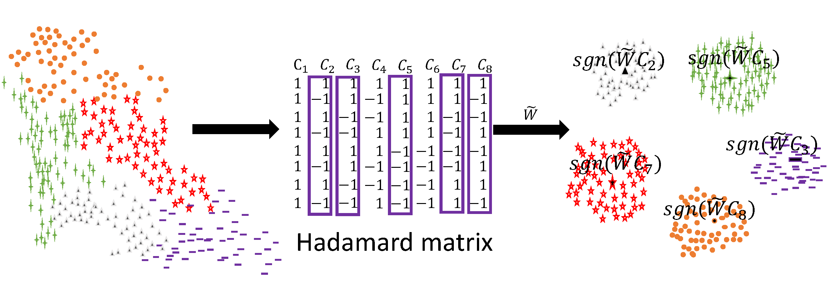
Figure 1. The framework of the proposed Hadamard Codebook based Online Hashing (HCOH). When new stream data from new class in left part is received, a column vector (codeword) in Hadamard matrix is sampled as a virtual multi-label representation​ to this class. Otherwise, it shares the same virtual multi-label representation​ with instances falling in the same class (denoted with different shapes in different colors). These virtual representations​ form the codebook $C$ (purple boxes). Then, a random​ Gaussian matrix $\tilde{W}$ is applied to reduce the codeword length to being consistent to the predefined hash bits. In sum, HCOH explicitly aggregates the undiscriminating features in the original space into discerning Hamming space (in the right part).

In this paper, we propose a simple and effective online hashing method, termed Hadamard Codebook based Online Hashing (HCOH), which aims to solve all aforementioned problems in a unified framework. First, we generate the Hadamard matrix via it definition, from which a discrete codebook is randomly sampled. Each codeword in such a codebook will be designated as the centroid of data sharing the same label, which can be used to conduct the learning of hash functions. Second, we employ the locality sensitive hashing (LSH) (Gionis et al., 1999) to reduce the codeword length to being consistent with the length of hash bits. Therefore, HCOH can train the objective function by leveraging the difference between the codewords and the produced Hamming codes, ​ and the hash functions are updated swiftly in an iterative manner with streaming data. Note that, both Hadamard matrix and the application of LSH can be efficiently applied online, because Hadamard matrix can be generated offline and the LSH is the data-independent encoding method with random projections.

No extra time is spent during online learning by using this method, which differentiates our method from the existing OH method (Cakir et al., 2017a), where the codebook has to be generated on-the-fly or to be in a fixed size. Moreover, the proposed HCOH by nature enables the embedding of supervised labels by using discriminative Hadamard matrix. Finally, in optimization, we show that the proposed HCOH needs only one instance to update each round, while most OH methods (Huang et al., 2013; Leng et al., 2015; Cakir and Sclaroff, 2015; Cakir et al., 2017b) need at least two instances. Extensive experiments on three benchmarks, i.e., CIFAR-10, Places205, and MNIST, show that the proposed HCOH achieves better or competitive results to the state-of-the-art methods (Huang et al., 2013; Leng et al., 2015; Cakir and Sclaroff, 2015; Cakir et al., 2017a, b).

The main contributions of this work are as follows:

1. A codeword sampled from Hadamard matrix is introduced as the centroid of different class labels, which can be utilized to learn discriminative binary codes in online manner.

2. Each codeword can be used as the virtual multi-label representation, which serves as the supervised information to build our effective model for online learning.

3. The specific stochastic gradient descent (SGD) is derived to achieve efficient optimization for the proposed method.

4. The proposed scheme achieves competitive results compared with several state-of-the-art online hashing (Huang et al., 2013; Leng et al., 2015; Cakir and Sclaroff, 2015; Cakir et al., 2017a, b).

​

2. Related Work

Recently, online hashing (OH) has received wide attention in online applications. It merits in efficiently updating the hash functions by using the streaming data online, which can be further subdivided into two categories: SGD-based OH methods (Huang et al., 2013; Cakir and Sclaroff, 2015; Cakir et al., 2017b, a), and matrix sketch-based OH methods (Leng et al., 2015).

For SGD-based online hashing, Online Kernel Hashing (OKH) (Huang et al., 2013) is the first of its kind, which updates hash functions with an online passive-aggressive algorithm (Crammer et al., 2006). OKH needs the new data to arrive in pairs with a similarity indicator, and the hash functions are updated via gradient descent on the selected hashing parameters. Similar to OKH, Adaptive Hashing (AdaptHash) (Cakir and Sclaroff, 2015) uses a similar framework, in which data are fed with pairs and label similarity. It defines a ​ hinge loss function and uses SGD to optimize model in online manner. Furthermore, Cakir et al. developed a more general two-step OH framework, a.k.a. Online Supervised Hashing (OSH) (Cakir et al., 2017a). In details of OSH, ​ Error Correcting Output Codes (ECOCs) (Dietterich and Bakiri, 1995) are first generated as the codebook, in which each codeword is further assigned to each​ class. Then, an exponential loss is developed to replace the $0\backslash 1$ loss, which is optimized via SGD to ensure the learned hash functions to fit the binary ECOCs. In (Cakir et al., 2017b), Online Hashing with Mutual Information (MIHash) was proposed by giving an image along with its neighbors and non-neighbors. It targets at optimizing the mutual information to reduce the ambiguity in the induced neighborhood structure in the Hamming space. Therefore, the whole framework can be optimized via SGD on mini-batch data.

For sketch-based online hashing, the main motivation comes from the idea of “data sketching”, which preserves the main property of a dataset with a significantly smaller size (Clarkson and Woodruff, 2009; Liberty, 2013). Leng et al. proposed Online Sketching Hashing (SketchHash) (Leng et al., 2015) where an online sketching with zero mean is developed to efficiently update hash codes online. An efficient variant of SVD decomposition (denoted as RSVD) (Sproston, 1980) is employed to obtain the hash functions. Although SketchHash (Leng et al., 2015) only requires $O(dl)$ space complexity to store and perform calculations on the streaming data, its time complexity is $O(ndl+dl^{2})$ to yield hash functions, where $n$ is the data size, $d$ is the data dimension, and $l$ denotes the sketching size satisfying $l<d\ll n$. Moreover, FasteR Online Sketching Hashing (FROSH) (Chen et al., 2017) was developed to further reduce the training time to $O(nl^{2}+nd)$. FROSH employs the independent Subsampled Randomized Hadamard Transform (SRHT) on different small data chunks to make the sketching compact and accurate, as well as to accelerate the sketching process.

3. The PROPOSED METHOD

3.1. Notations

In this section, we introduce the proposed Hadamard Codebook based Online Hashing (HCOH) in details. We first give notations used in the rest of this paper. We define $X=[x_{1},...,x_{n}]$ as a set of $n$ training data with the corresponding labels $Y=\{y_{1},...,y_{n}\}$, where each $x_{i}\in\mathbb{R}^{d}$ is the $i$-th $d$-dimensional feature with label $y_{i}\in\mathbb{R}$. Let $\mathcal{H}_{1}=\{-1,1\}^{r}$ be the $r-$dimensional Hamming space.

The goal of hashing is to assign each instance a binary code in $\mathcal{H}_{1}$, such that similarities in the original space are preserved in the Hamming space. This is achieved by learning a collection of hash functions $F=\{f_{1},...,f_{k},...,f_{r}\}$, where each function $f_{k}:\mathbb{R}^{d}\rightarrow\{-1,+1\}$ is to generate one bit code. As for online hashing, the hash functions $F$ are continuously updated from the input streaming data. Following (Chen et al., 2017), we mainly consider the linear projection-based hash function, where hash function for each bit is defined as:

$$f_{k}(x)=\mathrm{sgn}(w_{k}^{T}x+b_{k})=\begin{cases}$ 1$,&\mathrm{if}~{}w_{k}^{T}x+b_{k}\geq 0,\\ $-1$,&\mathrm{otherwise},\end{cases}$$

where $w_{k}\in\mathbb{R}^{d}$ is a parameter vector and $b_{k}\in\mathbb{R}$ is a bias term. Consequently, the hash codes for $X$ can be presented as

(1) $$F(X)=[f_{1}(X),...,f_{r}(X)]=\mathrm{sgn}(W^{T}X+b)\subset\mathbb{R}^{r\times n},$$

where $W=[w_{1},w_{2},...,w_{r}]\in\mathbb{R}^{d\times r}$ and $b=[b_{1};b_{2};...;b_{r}]\in\mathbb{R}^{r}$.

3.2. Online Hashing Formulation

To update the hash functions $F$ from streaming data online, the current mapping matrix $W^{t}$ and bias vector $b^{t}$ are learned on the $t$-th round input streaming data $X^{t}=[x^{t}_{1},...,x^{t}_{n^{t}}]\in\mathbb{R}^{d\times n^{t}}$ with their corresponding class labels $Y^{t}=\{y_{1}^{t},...,y^{t}_{n^{t}}\}\in\mathbb{R}^{n^{t}}$. As mentioned, the existing online hashing methods (Leng et al., 2015; Huang et al., 2013; Cakir et al., 2017b) requires the input data to be paired or batched, i.e., $n^{t}\geq 2$, for dynamic updating. In this paper, we ​ break through such a limitation by updating the model using only one instance via stochastic gradient descend, which is experimentally demonstrated to be very effective.

To this end, we first revisit SGD-based online hashing, i.e., an SGD version of the supervised hashing with error correcting codes (ECC) (Cakir et al., 2017a), known as “codebook”. Each vector, known as “codeword” in this codebook is assigned to the data falling into the same label. SGD-based hashing employs a $0\!-\!1$ loss function, which outputs either $1$ or $0$ to indicate whether the binary code generated by the existing hash functions is matched to the codeword. After replacing the $0\!-\!1$ loss with a convex loss function and relaxing the sign function, SGD is applied to minimize the loss and update the hash functions online. However, such methods cannot guarantee a constant loss upper bound (Huang et al., 2013), which is caused by the random construction of the codebook for class label. To compensate, a boosting scheme that considers previous mappings when updating each hash function is used to handle the error-correlation, which however needs more training time for each round input.

To solve the above mentioned problems, we argue that a better ECC ​ is the key for robust and efficient online hashing. The basic idea of ECC stems from the model of signal transmission in the communication field (Peterson and Weldon, 1972). Recently, ECC has become one of the most widely used strategies for dealing with multi-class classification problems, which contains both encoding and decoding phases. In the encoding phase, an encoding matrix (codebook) $C\in\{-1,1\}^{r^{*}\times N}$ decouples an $N$-class classification problem into $r^{*}$ binary-classification (bi-classification) problems (Liu et al., 2016). ​ That is, each column (codeword) of the matrix $C$ represents a class sample, each row represents a virtual category, and each original class can be approximated by a series of virtual categories in the decoding phase. Therefore, we argue that ECC can also help to solve the existing problems of online hashing, where the hash functions can be seen as a set of bi-classification models, and each $f_{k}(x_{i})=1$ means a given $x_{i}$ belongs to the $k$-th virtual ​catogory and vice versa.

Following the above definitions, we consider the linear regression to ​build each bi-classification model at the $t$-th round with the $i$-th new data point $x_{i}^{t}$:

(2) $$l(x_{i}^{t};W^{t})=\|F(x_{i}^{t})-c_{J(x_{i}^{t})}\|_{\mathcal{F}}^{2},$$

where $c_{i}$ is the $i$-th column of matrix $C$, and $J(x_{i}^{t})$ returns the class label of $x_{i}^{t}$, and $\|\cdot\|_{\mathcal{F}}$ is the Frobenius norm of the matrix. Therefore, the overall objective function can be rewritten as:

$$\min_{X^{t};W^{t},b^{t}}\!\!\!\!L(W^{t},b^{t}) \!=\!\frac{1}{n}\sum_{i=1}^{n}l(x_{i}^{t};W^{t},b^{t})\!=\!\frac{1}{n}\sum_{i=1}^{n}\|F(x_{i}^{t})-c_{J(x_{i}^{t})}\|_{\mathcal{F}}^{2}$$

(3) $$=\frac{1}{n}\|F(X^{t})-C_{J(X^{t})}\|_{\mathcal{F}}^{2},$$

where ​ $C_{J(X^{t})}\in\mathbb{R}^{r^{*}\times n^{t}}$ is the virtual multi-label representation matrix, of which the rows represent the virtual labels and the columns represent the samples.

However, the length of hash bit may not be the same with the length of codeword, i.e., $r\neq r^{*}$, which makes Eq. 3.2 hard to be directly optimized. To handle this problem, we further use the locality sensitive hashing (LSH) to transform the virtual labels to obtain the same length of binary codes to learn the hash functions. As proven in (Ding et al., 2016), LSH preserves the semantic similarity among label-based representation, since the collision probability between the binary codes of two labels is less than 0.5 if they are dissimilar, otherwise the collision is greater than 0.5. As a result, we reformulate Eq. 3.2 by LSH-based random hashing as:

(4) $$\min_{W^{t},b^{t}}\frac{1}{n}\Big{\|}F(X^{t})-\mathrm{sgn}\big{(}\tilde{W}^{T}C_{J(X^{t})}\big{)}\Big{\|}_{\mathcal{F}}^{2},$$

where $\tilde{W}\in\mathbf{R}^{r^{*}\times r}$ is the random Gaussian matrix.

3.3. Hadamard Codebook

As above, the key issue falls in the construction of encoding matrix (codebook) $C$. Towards learning an optimal matrix $C$ via ECC method, the following principles should be satisfied in traditional ECC: 1) Maximize the Hamming distance between each row, which allows strong error-correction ability. 2) Maximize the Hamming distance between each column, which ensures significant difference between the classifiers. However, the existing ECC construction schemes are too complex for generating long hash bits, which hinders their practical applications.

To solve this problem, we use the classical Hadamard codes in the communication system to construct ECC, which satisfies the above two principles (Horadam, 2012). In particular the Hadamard is an $n$-order orthogonal matrix, i.e., both its row vectors and columns vectors are pair-wise orthogonal, which by nature satisfies principles $1)$ and $2)$, respectively. And its elements are either $+1$ or $-1$. That is:

(5) $$CC^{T}=nI_{n},~{}\mathrm{or}~{}C^{T}C=nI_{n},$$

where $I_{n}$ is an $n-$order identity matrix.

Though the existence of Hadamard matrices of other orders (Paley, 1933; Williamson et al., 1944; Goldberg, 1966; Ockwig et al., 2005), we utilize $2^{k}$-order Hadamard matrices in this paper, which can achieve satisfactory performances as shown in Sec. 4. To construct the $2^{k}$-order Hadamard matrices, the entry in the $i$-th row and the $j$-th column can be defined as:

(6) $$C_{ij}=(-1)^{(i-1)\times(j-1)}.$$

Based on the definition of Hadamard matrix in Eq. 5, vectors in a Hadamard matrix are linearly independent. That is, Hadamard matrices can be well utilized as a discriminative set in Hamming space, which can further guide the learning of hash functions.

By the definition of $2^{k}$-order Hadamard matrix, we set the coding length $r^{*}$ as follows:

(7) $$r^{*}=\min\{l|l=2^{k},l\geq r,l\geq|Y|,k=1,2,3,...\},$$

where $|Y|$ is the number of class labels in the dataset. Therefore, we construct the square encoding matrix as $C_{r^{*}}\in\{-1,1\}^{r^{*}\times r^{*}}$. If a new data with new label is received, we randomly and non-repeatedly select a column representation to construct a virtual multi-label vector for this data. Otherwise, the virtual label previously assigned to the instances with the same label is given. Such vectors are further aggregated to construct the encoding matrix $C$. Therefore, our scheme does not need to predefine the category number of the dataset. The detailed framework can be shown in Fig. 1.

3.4. Learning Formulation

By giving the encoding matrix $C$ as defined in Sec. 3.3, we aim to optimize the objective function in Eq. 4. However, the sign function $\mathrm{sgn}(\cdot)$ is non-smooth and non-convex, which makes the standard optimization method infeasible for the proposed model. Following the work in (Liu et al., 2017), we relax the hash function $F(X)=\mathrm{sgn}(W^{T}X+b)$ as follows:

(8) $$\hat{F}(X)=\tanh(W^{T}X+b),$$

where $\tanh(\cdot)$ is the hyperbolic tangent function that transforms the discrete values $\{-1,+1\}$ to continuous values $(-1,+1)$.

Based on this relaxation, Eq. 2 can be reformulated as:

(9) $$\hat{L}(x_{i}^{t};W^{t},b^{t})=\|\hat{F}(x_{i}^{t})-c_{J(x_{i}^{t})}\|_{\mathcal{F}}^{2},$$

Ideally, SGD optimization can be used to carry out in an iterative way for Eq. 4, where the partial derivative of $\hat{L}$ with regard to $W$ and $b$ can be derived as:

(10) $$W^{t+1}\leftarrow W^{t}-\eta^{t}\frac{\partial\hat{L}(W^{t})}{\partial W^{t}},$$

(11) $$b^{t+1}\leftarrow W^{t}-\eta^{t}\frac{\partial\hat{L}(b^{t})}{\partial b^{t}},$$

where $\eta^{t}$ is a positive learning rate at the $t$-th round, and the derivative of $\hat{L}(W^{t})$ with respect to $W^{t}$ is

(12) $$\frac{\partial\hat{L}(W^{t})}{\partial W^{t}}=\frac{2}{n^{t}}X^{t}\Big{(}\big{(}\tanh({W^{t}}^{T}X^{t}+b^{t})-\mathrm{LSH}(X^{t})\big{)}\odot P\Big{)},$$

and the derivative of $\hat{b^{t}}$ with respect to $b^{t}$ is

(13) $$\frac{\partial\hat{L}(b^{t})}{\partial b^{t}}=\frac{2}{n^{t}}\Big{(}\big{(}\tanh({W^{t}}^{T}X^{t}+b^{t})-\mathrm{LSH}(X^{t})\big{)}\odot P\Big{)},$$

where $P=\big{(}1-tanh({W^{t}}^{T}X^{t}+b^{t})\big{)}\odot tanh({W^{t}}^{T}X^{t}+b^{t})$, $\odot$ denotes the element-wise product, and $\mathrm{LSH}(X^{t})=\mathrm{sgn}\big{(}\tilde{W}^{T}C_{J(X^{t})}\big{)}$. We summarize our proposed HOCH in Alg.1.

Algorithm 1 Hadamard Codebook Hashing based Online Hashing (HCOH)

0:  Training data set $D$ with feature space $X$ and label space $Y$, the number of hash bits $r$, the learning rate $\eta$, the total number of streaming data batches $L$.

0:  The hash codes $B$ for training space $X$ and the projection coefficient matrix $\mathbf{W}$.

1:  Initialize $W_{1}$ and $b_{1}$ with the normal Gaussian distribution.

2:  Set the value of $r^{*}$ by Eq. 7.

3:  Generate Hadamard matrix as stated in Sec. 3.3.

4:  if $r=r^{*}$ then

5:     Set $\tilde{W}$ as an identity matrix.

6:  else

7:     Randomize $\tilde{W}$ from Gaussian distribution.

8:  end if

9:  for $t=1\to L$ do

10:     Update $W^{t}$ by Eq. 12.

11:     Update $b^{t}$ by Eq. 13.

12:  end for

13:  Compute $B=sgn(W^{T}X+b).$

Table 1. mAP and Precision@500 Comparisons on CIFAR-10 with 8, 16, 32, 64 and 128 bits.

Method	mAP					Precision@500
	8-bit	16-bit	32-bit	64-it	128-bit	8-bit	16-bit	32-bit	64-bit	128-bit
OKH	0.100	0.134	0.223	0.268	0.350	0.100	0.179	0.361	0.431	0.510
SketchHash	0.248	0.301	0.302	-	-	0.348	0.433	0.450	-	-
AdaptHash	0.116	0.138	0.216	0.305	0.293	0.129	0.182	0.357	0.464	0.467
OSH	0.123	0.126	0.129	0.127	0.125	0.138	0.150	0.150	0.154	0.157
MIHash	0.512	0.640	0.675	0.667	0.664	0.560	0.703	0.744	0.739	0.745
HCOH	0.536	0.698	0.688	0.724	0.734	0.636	0.752	0.756	0.772	0.779

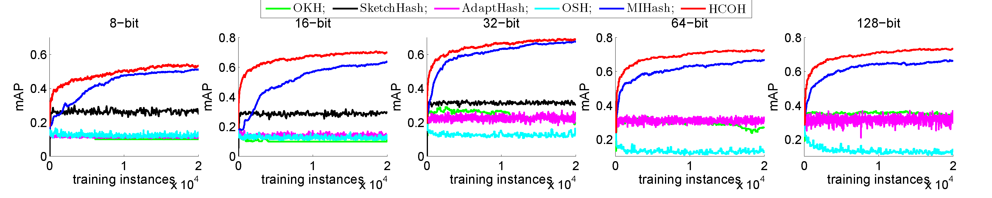
Figure 2. mAP performance with respect to different number of training instances on CIFAR-10.

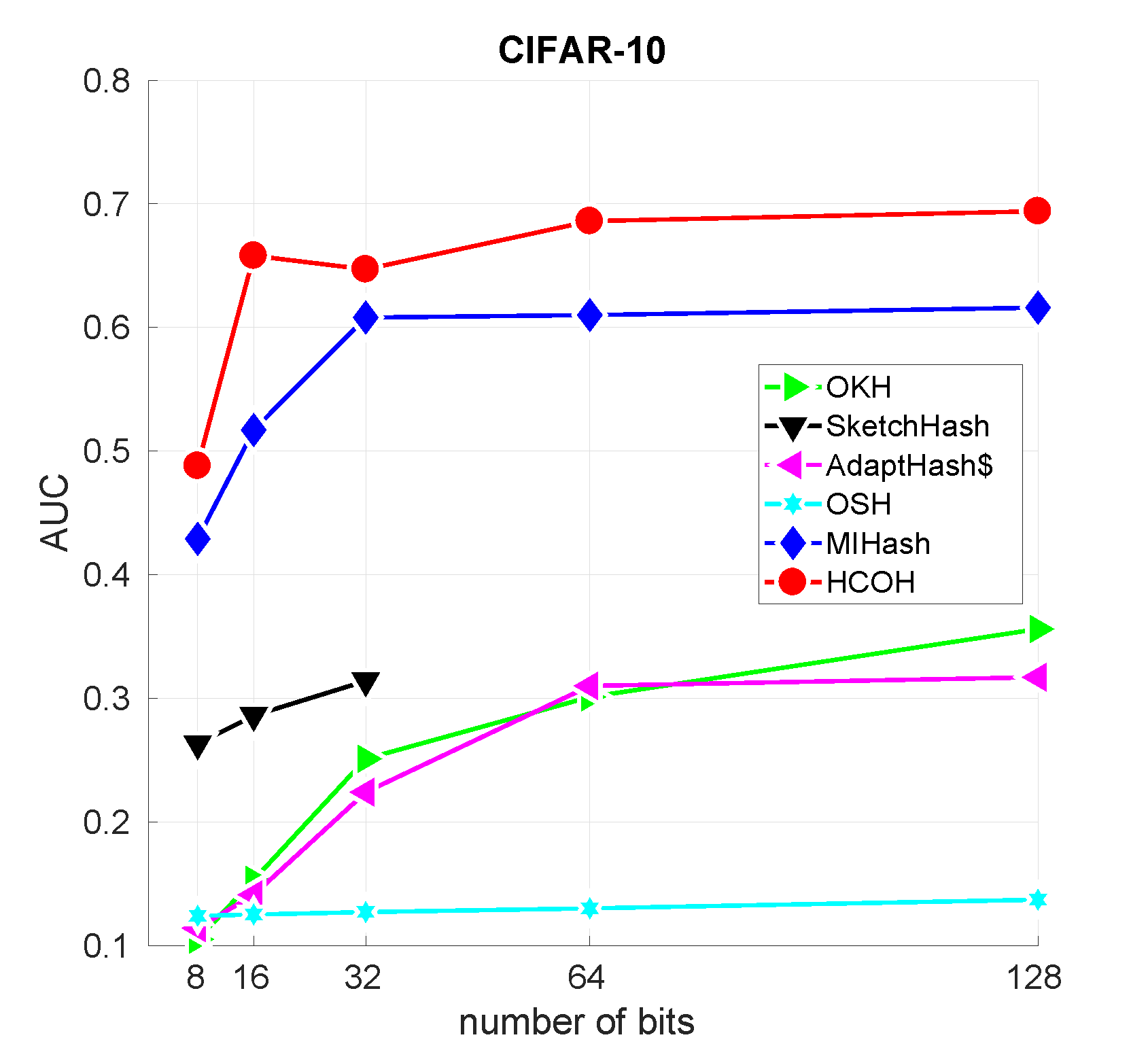
Figure 3. AUC performance with respect to different lengths of hash bits on CIFAR-10.

4. EXPERIMENTS

In this section, we report our quantitative experiments to verify the effectiveness and efficiency of the proposed method. We run large-scale image retrieval experiments on three datasets, i.e., CIFAR-10 (Krizhevsky and Hinton, 2009), Places205 (Zhou et al., 2014), and MNIST (LeCun et al., 1998).

4.1. Datasets

CIFAR-10 is a widely-used dataset for image classification and retrieval. It contains 60K samples from 10 categories represented by 4096-dimentional CNN features extracted from the fc-7 layer of a VGG-16 network (Simonyan and Zisserman, 2014) pre-trained on ImageNet. As in (Cakir et al., 2017b), the entire dataset is partitioned into two parts: a retrieval set with 59K samples, and a test set with 1K samples. And a random subset of 20K images from the retrieval set is used for learning hash functions.

Places205 is a 2.5-million image set where each instance belongs to one of 205 scene categories. Following (Cakir et al., 2017b, a), features are pre-computed from the fc-7 layer of an AlexNet (Krizhevsky et al., 2012), and then further reduced by PCA to a 128-dimension vector. For each category, 20 instances are randomly sampled to form a test set, and the remaining are used to form a retrieval set. We sample a subset from the retrieval set with 100K images at random for learning hash functions.

MNIST dataset contains 70K images of handwritten digits with 10 classes. Feature vectors are presented by $28\times 28=784$ normalized original pixels. We construct the test set by sampling $100$ instances from each class and the other are used as retrieval set. From the retrieval set, $20K$ instances are adopted to learn the hash functions.

4.2. Evaluation Protocols and Baselines

As for the evaluation protocols, we adopt the widely-used mean Average Precision (mAP) at varying bit lengths, as well as the mean precision of the top $500$ retrieved samples (denoted as Precision@500). We also report the mAP vs. numbers of training instances, as well as its corresponding area under the mAP curve (denoted as AUC). Due to the large scale of Places205 benchmark, it is very time-consuming to compute mAP. Following (Cakir et al., 2017b), we only compute mAP on the top $1000$ retrieved samples (Denoted as mAP@1000).

We compare our method with five state-of-the-art online hashing algorithms, i.e., Online Kernel Hashing (OKH) (Huang et al., 2013), Online Sketching Hashing (SketchHash) (Leng et al., 2015), Adaptive Hashing (AdaptHash) (Cakir and Sclaroff, 2015), Online Supervised Hashing (OSH) (Cakir et al., 2017a) and Online Hashing with Mutual Information (MIHash) (Cakir et al., 2017b). Source codes of all these methods are available publicly. Our model is implemented with MATLAB. Training is done on a standard workstation with a 3.6GHz Intel Core I7 4790 CPU and 16G RAM. All the experimental results are averaged over three runs.

Table 2. mAP@1000 and Precision@500 Comparisons on Places205 with 8, 16, 32, 64 and 128 bits.

Method	mAP@1000					Precision@500
	8-bit	16-bit	32-bit	64-bit	128-bit	8-bit	16-bit	32-bit	64-bit	128-bit
OKH	0.018	0.033	0.122	0.114	0.258	0.011	0.025	0.104	0.094	0.091
SketchHash	0.052	0.120	0.202	-	-	0.045	0.108	0.186	-	-
AdaptHash	0.028	0.097	0.195	0.222	0.229	0.029	0.089	0.178	0.243	0.285
OSH	0.018	0.021	0.022	0.043	0.164	0.010	0.012	0.014	0.029	0.132
MIHash	0.094	0.191	0.244	0.308	0.332	0.083	0.179	0.245	0.282	0.313
HCOH	0.049	0.173	0.259	0.321	0.347	0.063	0.147	0.256	0.298	0.324

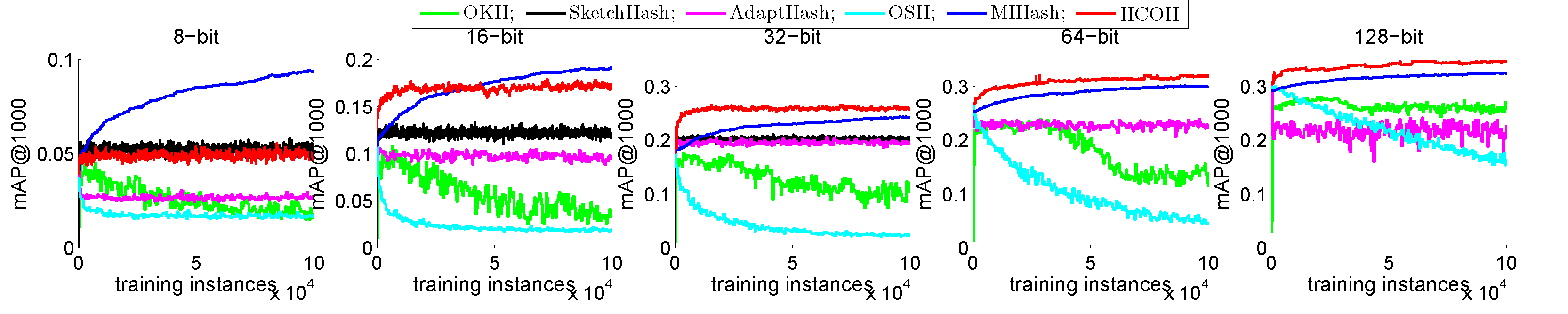
Figure 4. mAP performance with respect to different number of training instances on Places205.

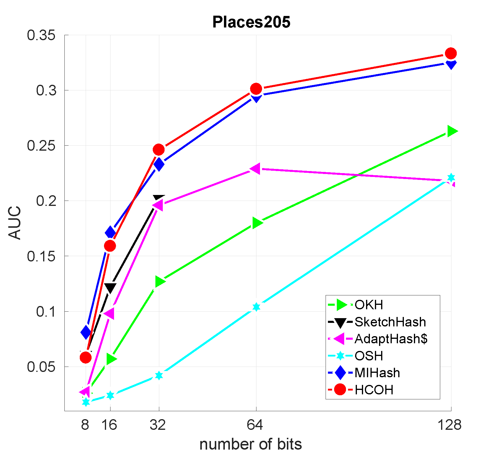
Figure 5. AUC performance with respect to different lengths of hash bits on Places205.

4.3. Parametric Settings

We describe the parameters to be tuned during the experiments. Due to that we share the common dataset configurations on CIFAR-10 and Places205, we directly adopt the parameters as described in (Cakir et al., 2017b) for all baselines. Otherwise, we partition a validate set from training set with a size of 2K, 10K, 2K for CIFAR-10, Places205 and MINST, respectively, and identify the best choice for each parameter. The following describes our parameter settings.

• OKH: The tuple $(C,\alpha)$ is set as $(0.001,0.3)$, $(0.0001,0.7)$ and $(0.001,0.3)$ for CIFAR-10, Places205 and MNIST, respectively.

• SketchHash: The tuple $(sketchsize,batchsize)$ is set to $(200,\allowbreak 50)$, $(100,50)$ and $(200,50)$ for CIFAR-10, Places205 and MNIST, respectively.

• AdaptHash: The tuple $(\alpha,\lambda,\eta)$ is set as $(0.9,0.01,0.1)$, $(0.9,\allowbreak 0.01,0.1)$ and $(0.8,0.01,0.2)$ for CIFAR-10, Places205 and MNIST, respectively.

• OSH: For all datasets, $\eta$ is set to $0.1$ and the ECOC codebook $C$ is populated the same way as in (Cakir et al., 2017a).

• MIHash: The tuple $(\theta,\mathcal{R},A)$ as $(0,1000,10)$, $(0,5000,10)$ and $(0,1000,10)$ for CIFAR-10, Places205 and MNIST, respectively.

Due to the page limit, we do not explicitly explain the meaning of these parameters. Detailed information can be found in the corresponding papers (Huang et al., 2013; Leng et al., 2015; Cakir and Sclaroff, 2015; Cakir et al., 2017a, b). Also, for SketchHash, the batch size has to be larger than the length of hash bits. Therefore, we do not report its performance when the hash bits are $64$ and $128$.

4.4. Results and Discussions

4.4.1. Results on CIFAR-10

We first report the performance of the proposed method on CIFAR-10. Tab. 1 illustrates the mAP and Precision@500 of our method and the baselines with different hash bits. Fig. 2 reports the mAP with respect to different numbers of training instances, and Fig. 3 displays the corresponding AUC results when the hash bits are $8$, $16$, $32$, $64$ and $128$. We can see that the proposed method outperforms all of the other methods in all cases.

In terms of mAP and Precision@500, we can observe that the proposed method achieves substantially better performance at all code lengths. Comparing to the state-of-the-art method, i.e., MIHash, the proposed method shows a relative increase of $4.69\%$, $9.06\%$, $1.93\%$, $8.55\%$, $10.54\%$ for mAP when hash bits are $8$, $16$, $32$, $64$, $128$, respectively, as well as $13.57\%$, $6.97\%$, $1.61\%$, $4.47\%$, $4.56\%$ for Precision@500 when hash bits are $8$, $16$, $32$, $64$, $128$, respectively. As for the mAP performance with respect to different numbers of training instances, the proposed method not only surpasses the state-of-the-art methods by a large margin, but also achieves satisfactory performance with less training instances. Taking the metric under 64-bit as an example, the proposed method obtains 0.6 mAP when the training instances grow to around $1K$, while it takes MIHash nearly $8K$ instances to achieve the same mAP. For a deeper look, we further analyze the area under the mAP curves in Fig. 3. Among all baselines including OSH that uses ECOC as a codebook, the proposed HCOH always achieves the best results, which implies that using Hadamard codebook with our proposed online learning scheme is more preferable than using ECOC with classical SGD learning scheme.

Table 3. mAP and Precision@500 Comparisons on MNIST with 8, 16, 32, 64 and 128 bits.

Method	mAP					Precision@500
	8-bit	16-bit	32-bit	64-it	128-bit	8-bit	16-bit	32-bit	64-bit	128-bit
OKH	0.100	0.155	0.224	0.301	0.404	0.100	0.257	0.452	0.606	0.732
SketchHash	0.257	0.312	0.348	-	-	0.420	0.571	0.641	-	-
AdaptHash	0.138	0.207	0.319	0.292	0.208	0.187	0.368	0.571	0.558	0.439
OSH	0.130	0.144	0.130	0.146	0.143	0.152	0.171	0.165	0.222	0.224
MIHash	0.664	0.741	0.744	0.713	0.681	0.755	0.801	0.823	0.812	0.812
HCOH	0.536	0.708	0.756	0.759	0.771	0.662	0.801	0.837	0.848	0.854

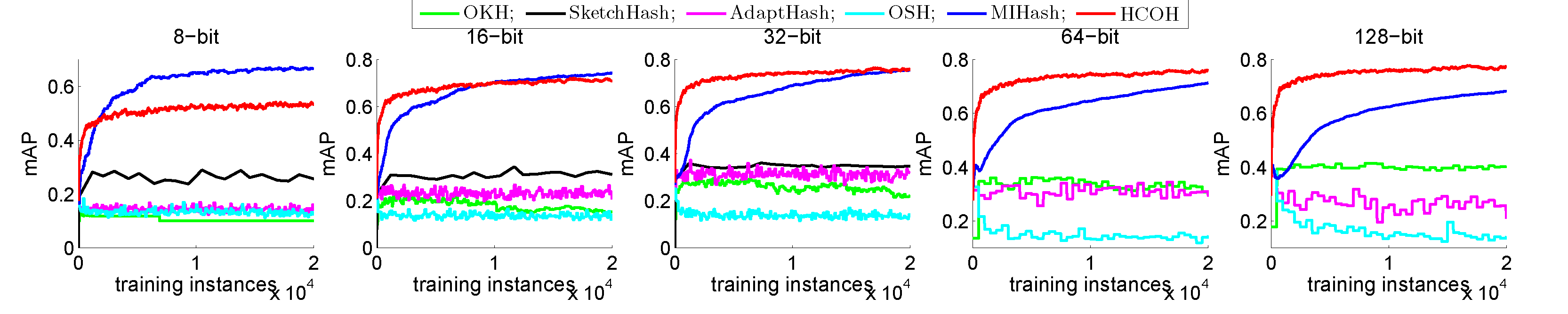
Figure 6. mAP performance with respect to different number of training instances on MNIST.

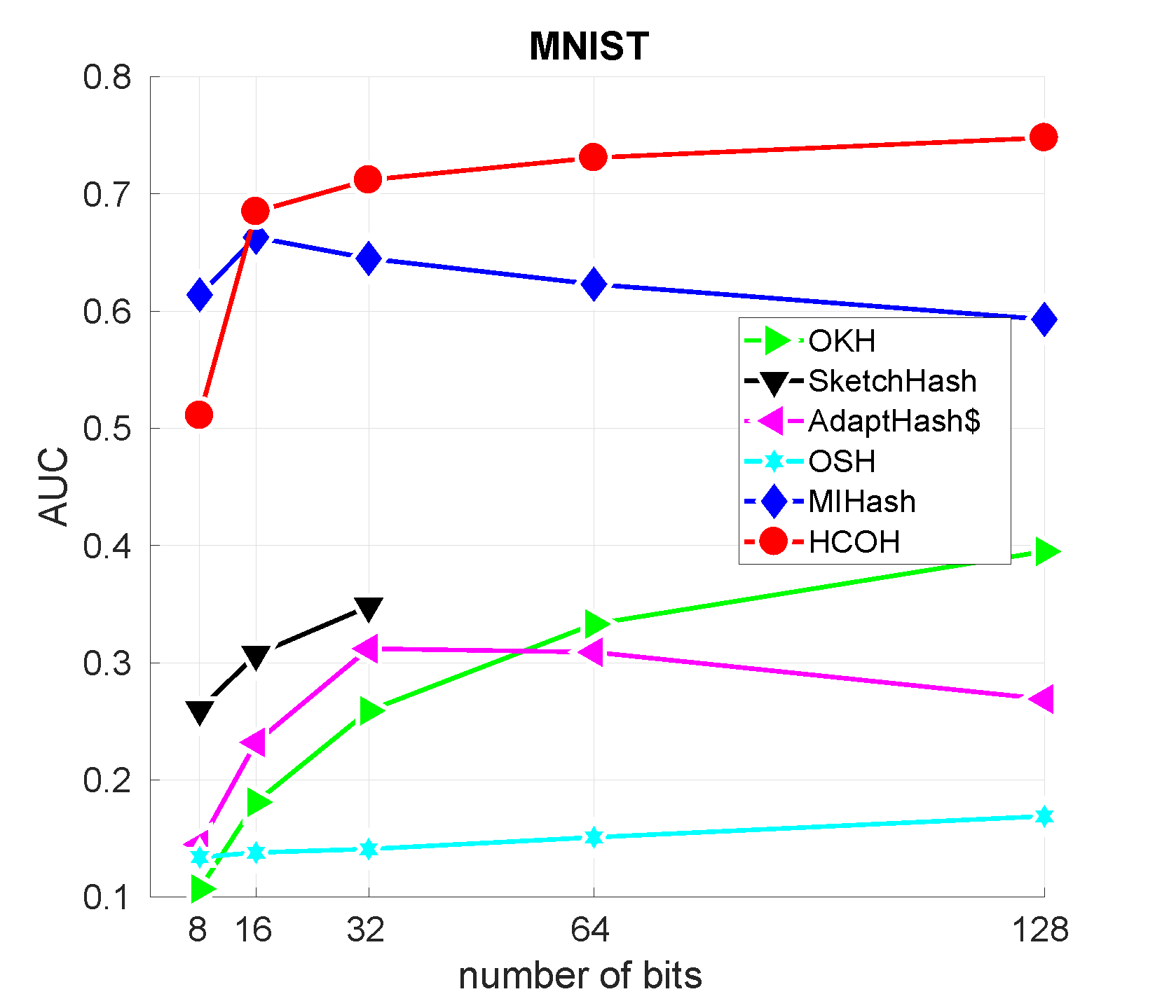
Figure 7. AUC performance with respect to different lengths of hash bits on MNIST.

4.4.2. Results on Places205

Tab. 2 shows comparative results about mAP@1000 and Precision@500 on a larger-scale dataset Places205 with different code lengths, respectively. The mAP with respect to different numbers of training instances and its AUC are reported in Fig. 4 and Fig. 5. We can find that in low bit cases, i.e., $16$-bit and $32$-bit, MIHash achieves the best results in all four metrics. However, as the length of hash bit grows, the proposed HCOH still outperforms all the baselines including MIHash, which claims that the overall performance of the HOCH is better on Places205.

In detail, in low bits of $8$ and $16$, compared with the proposed HCOH, MIHash acquires $23.88\%$, $4.66\%$ gains for mAP@1000 and $31.75\%$, $21.77\%$ gains for Precision@500, respectively. Notably, under the setting of $8$-bit, SketchHash is second best. When the hash bits are 32, 64 and 128, the proposed HCOH surpasses MIHash by $6.15\%$, $4.22\%$, $4.52\%$ gains for mAP@1000 and $4.49\%$, $5.67\%$, $3.51\%$ gains for Precision@500, respectively. We further look into the mAP with respect to different number of training instances and the AUC under different hash bits. As depicted in Fig. 4, when the lengths of hash codes are $8$ and $16$, at first, the proposed HCOH rapidly increase, and as the dataset grows, MIHash transcends. However, when referring to $32$-bit, $64$-bit and $128$-bit, the proposed HCOH keeps the first throughout the training process. In Fig. 5, it shows similar results as in Fig. 4. In the $8$-bit, $16$-bit settings, MIHash performs the best. Whereas, In the settings of $32$-bit, $64$-bit, $128$-bit, the proposed HCOH shows its dominance and keeps the first results.

To analyze the reason for unsatisfactory performance of the proposed HCOH in low hash bits, it owes to the usage of LSH to reduce the codeword’s length, because LSH needs longer codes to achieve the theoretic convergence guarantee (Gionis et al., 1999). Nevertheless, we argue that when facing large-scale datasets, longer binary codes are necessities to guarantee good performance. Even though MIHash shows best in hash bits of $8$ and $16$, the performance are far from satisfying. For example, in 8-bit setting, the $m$AP is only $0.094$, which is insufficient in real applications. However, when hash bit is $64$, the best result increases to $0.321$, which is more applicable. Therefore, longer binary codes are necessary to achieve workable performance in large-scale settings.

4.4.3. Results on MNIST

The mAP and Precision@500 for all methods on MNIST are listed in Tab. 3. The mAP with regard to different numbers of training instances and AUC curves are displayed in Fig. 6 and Fig. 7, respectively. We can observe that the results on MNIST are very similar to those on Places205. When it comes to low hash bits of $8$ and $16$, the performance of the proposed HCOH is worse than MIHash. But in most cases, our method surpasses all of the other methods. As aforementioned, low hash bits are not suitable for large-scale datasets, especially for streaming data due to its low performance.

In particular, when the hash bits are $8$ and $16$, MIHash gets $23.88\%$ and $0.05\%$ mAP gains to the proposed method. When hash bits are $32$, $64$ and $128$, the proposed HCOH gets $1.61\%$, $6.45\%$, $13.22\%$ mAP gains to MIHash. As for the Precision@500, MIHash gains $14.05\%$ higher than HCOH when the hash bit is $8$. Both the proposed HCOH and MIHash earn $0.801$ mAP under the hash bit of 16. Regarding to the hash bits of $32$, $64$, $128$, the proposed method consistently outperforms MIHash by $1.70\%$, $4.43\%$ and $5.17\%$ mAP gains, respectively. Further, we analyze the mAP with respect to different numbers of training instances and the corresponding AUC. As shown in Fig. 6, when the hash bit is $8$, the proposed method shows best mAP at first, but is surpassed by MIHash as the number of instances increases. Fig. 7 reports the same observation for AUC. Interestingly, in regard of the 16-bit case, even MIHash transcends the proposed HCOH in the end, but the proposed HCOH still holds the first position for AUC metric. For higher hash bits, the proposed method significantly surpasses all baselines by a large margin.

Based on Tab. 1, Tab. 2 and Tab. 3, it can be observed that when the hash bits are $8$ and $16$, HCOH is worse than MIHash on Places205 and MNIST, while HCOH performs better on CIFAR-10. We argue that this is owing to the dimensionality of features. As introduced in Sec 4.1, features in CIFAR-10 are 4096-D, while it is only 128-D and 784-D for Places205 and MNIST, respectively. So as to preserve mutual information in Hamming space, MIHash learns binary codes via linear mappings which suffers great quantization ​error when mapping data from high-dimensional space into low-bit Hamming space. Hence, we argue that when learning low-bit binary codings, $\mathbf{i.e.}$, $8$ or $16$ bits, our method is suitable for high-dimensional features, while MIHash is proper to low-dimensional features.

4.4.4. Parameter Sensitivity Analysis

We further analyze the ​ influence of hyper-parameters on the performance. Unlike other baselines, there are only two parameters in the proposed HCOH, i.e., the learning rate $\eta$ and the batch size $n$, which reflects another advantage of the proposed HCOH, because less parameters denote simpleness to complement and less time spent on deciding optimal values. For simplicity, at each round $t$, we set $\eta^{t}$ and $n^{t}$ as constants.

To validate the effectiveness of these two parameters, we conduct experiments on CIFAR-10 when the hash bit is 16. In Fig. 8(a), we plot the mAP curves under different values of learning rate. We can see that the mAP results fluctuate as the learning rate $\eta$ varies. This is owing to the random sampling process involved in the evaluation protocol. In general, when $\eta=0.2$, the proposed HCOH performs the best. Fig. 8(b) shows the mAP performance along with the increase of batch size $n$. Generally, the performance of the proposed HCOH degenerates with the increase of $n$. The precise results for $n^{t}=1$ and $n^{t}=2$ are 0.755 and 0.716, respectively. This is because individual update preserves more instance-level information. The best choice for $n$ is $1$ in such a case.

​Similarly, the same experiments can be conducted for Places205 and MNIST. In this paper, the tuple ($\eta$, $n$) is set as ($0.2$,$1$), ($0.1$,$1$) and ($0.2$, $1$) for CIFAR-10, Places205 and MNIST, respectively. Through the ​ analysis, we demonstrate that the proposed HCOH only needs one instance to update the hash functions each round, which differs HCOH to most OH methods, which needs at least two instances.

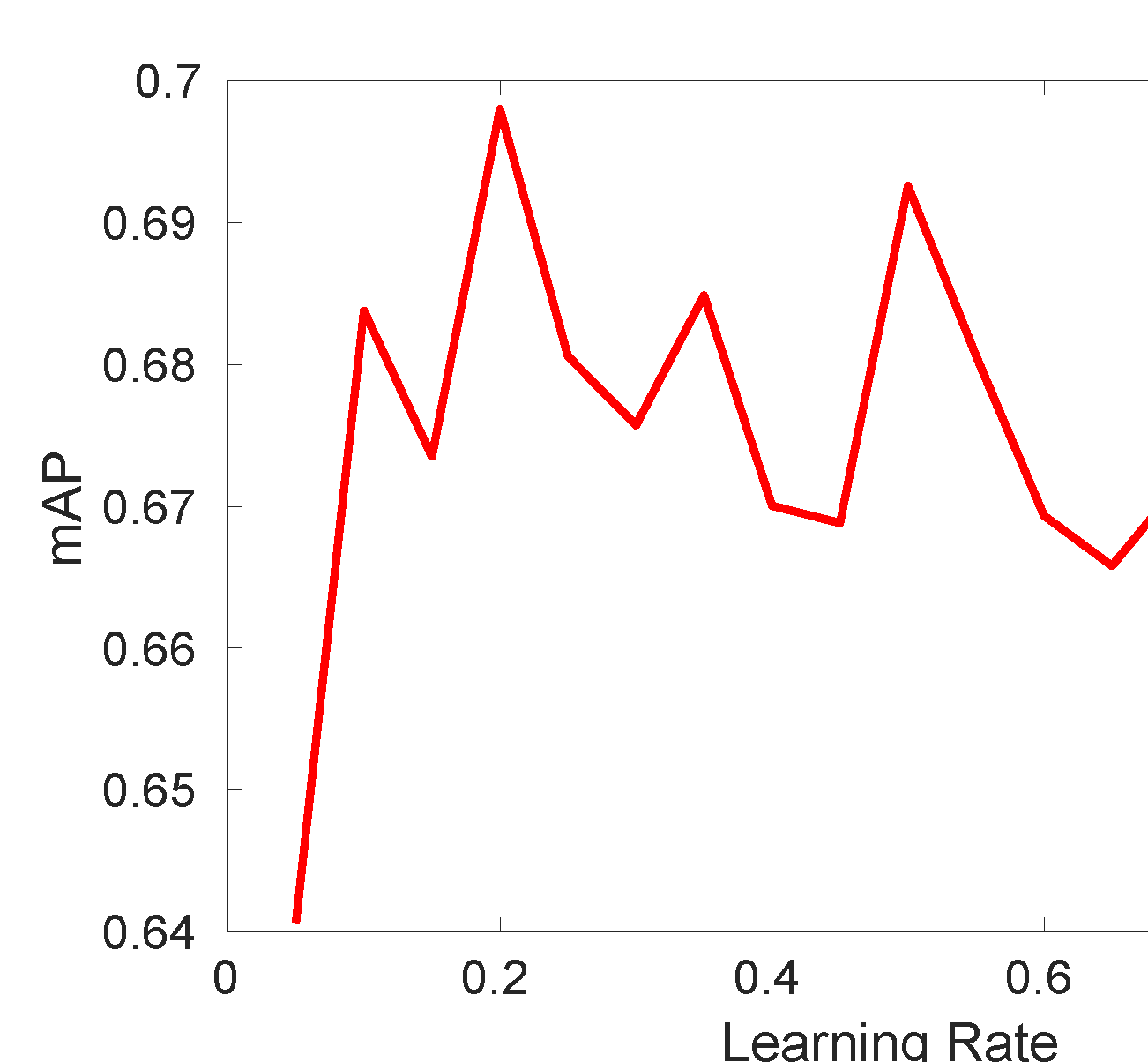
(a) mAP with varying learning rates.

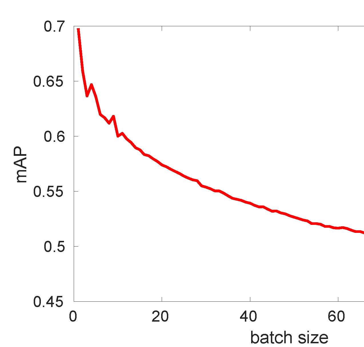
(b) mAP over different sizes of batch.

Figure 8. The analysis of hyper-parameters.

4.5. Time Complexity

To demonstrate the efficiency of the proposed HCOH, we further compare the training time on CIFAR-10 when the hash bit is $32$. The results are summarized in Tab. 4​ , which shows that HCOH has acceptable training time. Although OKH and SketchHash are more efficient, they suffer from unsatisfactory performance as analyzed in Sec. 4.4. When comparing to OSH, the proposed HCOH gains a $20.42\times$ training speed acceleration. To analyze, though OSH also adopts codebook-based scheme, it has to utilize the boosting algorithm to improve the performance, which increases the training time. Regarding to MIHash, the proposed HCOH obtains a $5.26\times$ training speed acceleration, which is due to the usage of mutual information, i.e., given a query, MHIash has to calculate the Hamming distance between its neighbors and non-neighbors. Even if in some situations of low hash bits, the performance of MIhash may surpass the proposed HCOH, it has unavoidably introduced more training time, which is in many cases unacceptable in OH​ .

Table 4. Training times on the CIFAR-10 with 20K training instances, under 32-bit hash codes.

Method	Training Time (s)
OKH	12.40
SketchHash	8.25
AdaptHash	78.52
OSH	333.70
MIHash	95.24
Ours	15.58

5. CONCLUSION

In this paper, we propose a robust supervised online hashing scheme, termed Hadamard Codebook based Online Hashing ​, which can be trained very efficiently online, and is not limited by predefining the category number of the streaming dataset. To this end, the proposed HCOH is firstly associated with a codebook sampled from the generated Hadamard matrices, and then designates the codeword in the codebook as the centroid of data sharing the same label space, so as to conduct the learning of hash functions. To keep consistency with the length of hash bits, locality sensitive hashing is further employed to reduce the codeword dimension. Stochastic gradient descend ​ is developed to update the hash codes for streaming data online. In optimization, the proposed HCOH only needs one training instance each round. Extensive experiments with quantitative evaluation metrics and benchmarks including CIFAR-10, Places-205, and MNIST demonstrate the merits of of the proposed method over the state-of-the-art.

6. Acknowledge

This work is supported by the National Key R&D Program (No. 2017YFC0113000, and No. 2016YFB1001503), Nature Science Foundation of China (No. U1705262, No. 61772443, and No. 61572410), Post Doctoral Innovative Talent Support Program under Grant BX201600094, China Post-Doctoral Science Foundation under Grant 2017M612134, Scientific Research Project of National Language Committee of China (Grant No. YB135-49), and Nature Science Foundation of Fujian Province, China (No. 2017J01125 and No. 2018J01106).

References

- (1)
- Cakir et al. (2017a) Fatih Cakir, Sarah Adel Bargal, and Stan Sclaroff. 2017a. Online supervised hashing. Computer Vision and Image Understanding (2017).
- Cakir et al. (2017b) Fatih Cakir, Kun He, Sarah Adel Bargal, and Stanley Sclaroff. 2017b. MIHash: Online hashing with mutual information. In Proceedings of the ICCV.
- Cakir and Sclaroff (2015) Fatih Cakir and Stan Sclaroff. 2015. Adaptive hashing for fast similarity search. In Proceedings of the ICCV.
- Chen et al. (2017) Xixian Chen, Irwin King, and Michael R. Lyu. 2017. FROSH: FasteR Online Sketching Hashing. In Proceedings of the UAI.
- Clarkson and Woodruff (2009) Kenneth L Clarkson and David P Woodruff. 2009. Numerical linear algebra in the streaming model. In Proceedings of the forty-first annual ACM symposium on Theory of computing.
- Crammer et al. (2006) Koby Crammer, Ofer Dekel, Joseph Keshet, Shai Shalev-Shwartz, and Yoram Singer. 2006. Online passive-aggressive algorithms. Journal of Machine Learning Research (2006).
- Crammer et al. (2004) Koby Crammer, Jaz Kandola, and Yoram Singer. 2004. Online classification on a budget. In Proceedings of the NIPS.
- Dietterich and Bakiri (1995) Thomas G Dietterich and Ghulum Bakiri. 1995. Solving multiclass learning problems via error-correcting output codes. Journal of artificial intelligence research (1995).
- Ding et al. (2016) Kun Ding, Chunlei Huo, Bin Fan, Shiming Xiang, and Chunhong Pan. 2016. In defense of locality-sensitive hashing. IEEE transactions on neural networks and learning systems (2016).
- Gionis et al. (1999) Aristides Gionis, Piotr Indyk, Rajeev Motwani, et al. 1999. Similarity search in high dimensions via hashing. In Proceedings of the Vldb.
- Goldberg (1966) Karl Goldberg. 1966. Hadamard matrices of order cube plus one. Proceedings of the AMS (1966).
- Gong et al. (2013) Yunchao Gong, Svetlana Lazebnik, Albert Gordo, and Florent Perronnin. 2013. Iterative quantization: A procrustean approach to learning binary codes for large-scale image retrieval. IEEE Transactions on Pattern Analysis and Machine Intelligence (2013).
- Heo et al. (2012) Jae-Pil Heo, Youngwoon Lee, Junfeng He, Shih-Fu Chang, and Sung-Eui Yoon. 2012. Spherical hashing. In Proceedings of the CVPR.
- Horadam (2012) Kathy J Horadam. 2012. Hadamard matrices and their applications. Princeton university press.
- Huang et al. (2013) Long-Kai Huang, Qiang Yang, and Wei-Shi Zheng. 2013. Online hashing. In Proceedings of the IJCAI.
- Jiang and Li (2018) Qing-Yuan Jiang and Wu-Jun Li. 2018. Asymmetric Deep Supervised Hashing. Proceedings of the AAAI (2018).
- Krizhevsky and Hinton (2009) Alex Krizhevsky and Geoffrey Hinton. 2009. Learning multiple layers of features from tiny images. Technical report, University of Toronto (2009).
- Krizhevsky et al. (2012) Alex Krizhevsky, Ilya Sutskever, and Geoffrey E Hinton. 2012. Imagenet classification with deep convolutional neural networks. In Proceedings of the NIPS.
- LeCun et al. (1998) Yann LeCun, Léon Bottou, Yoshua Bengio, and Patrick Haffner. 1998. Gradient-based learning applied to document recognition. Proc. IEEE (1998).
- Leng et al. (2015) Cong Leng, Jiaxiang Wu, Jian Cheng, Xiao Bai, and Hanqing Lu. 2015. Online sketching hashing. In Proceedings of the CVPR.
- Liberty (2013) Edo Liberty. 2013. Simple and deterministic matrix sketching. In Proceedings of the KDD.
- Liu et al. (2017) Hong Liu, Rongrong Ji, Yongjian Wu, and Feiyue Huang. 2017. Ordinal Constrained Binary Code Learning for Nearest Neighbor Search.. In Proceedings of the AAAI.
- Liu et al. (2016) Mingxia Liu, Daoqiang Zhang, Songcan Chen, and Hui Xue. 2016. Joint binary classifier learning for ECOC-based multi-class classification. IEEE Transactions on Pattern Analysis and Machine Intelligence (2016).
- Liu et al. (2014) Wei Liu, Cun Mu, Sanjiv Kumar, and Shih-Fu Chang. 2014. Discrete graph hashing. In Proceedings of the NIPS.
- Liu et al. (2012) Wei Liu, Jun Wang, Rongrong Ji, Yu-Gang Jiang, and Shih-Fu Chang. 2012. Supervised hashing with kernels. In Proceedings of the CVPR.
- Lu et al. (2017) Xiaoqiang Lu, Xiangtao Zheng, and Xuelong Li. 2017. Latent semantic minimal hashing for image retrieval. IEEE Transactions on Image Processing (2017).
- Ockwig et al. (2005) Nathan W Ockwig, Olaf Delgado-Friedrichs, Michael O’Keeffe, and Omar M Yaghi. 2005. Reticular chemistry: occurrence and taxonomy of nets and grammar for the design of frameworks. Accounts of chemical research (2005).
- Paley (1933) Raymond EAC Paley. 1933. On orthogonal matrices. Studies in Applied Mathematics (1933).
- Peterson and Weldon (1972) William Wesley Peterson and Edward J Weldon. 1972. Error-correcting codes. MIT press.
- Shalev-Shwartz et al. (2012) Shai Shalev-Shwartz et al. 2012. Online learning and online convex optimization. Foundations and Trends® in Machine Learning (2012).
- Shen et al. (2015) Fumin Shen, Chunhua Shen, Wei Liu, and Heng Tao Shen. 2015. Supervised Discrete Hashing.. In Proceedings of the CVPR.
- Simonyan and Zisserman (2014) Karen Simonyan and Andrew Zisserman. 2014. Very deep convolutional networks for large-scale image recognition. arXiv preprint arXiv:1409.1556 (2014).
- Sproston (1980) JL Sproston. 1980. Matrix computation for engineers and scientists. Pergamon.
- Wang et al. (2018) Jingdong Wang, Ting Zhang, Nicu Sebe, Heng Tao Shen, et al. 2018. A survey on learning to hash. IEEE Transactions on Pattern Analysis and Machine Intelligence (2018).
- Wang et al. (2014) Jialei Wang, Peilin Zhao, Steven CH Hoi, and Rong Jin. 2014. Online feature selection and its applications. IEEE Transactions on Knowledge and Data Engineering (2014).
- Weiss et al. (2009) Yair Weiss, Antonio Torralba, and Rob Fergus. 2009. Spectral hashing. In Proceedings of the NIPS.
- Williamson et al. (1944) John Williamson et al. 1944. Hadamard’s determinant theorem and the sum of four squares. Duke Mathematical Journal (1944).
- Zhou et al. (2014) Bolei Zhou, Agata Lapedriza, Jianxiong Xiao, Antonio Torralba, and Aude Oliva. 2014. Learning deep features for scene recognition using places database. In Proceedings of the NIPS.