Self-similar analysis of a viscous heated Oberbeck-Boussinesq flow system

Abstract

The simplest model to couple the heat conduction and Navier-Stokes equations together is the Oberbeck-Boussinesq(OB) system which were investigated by E.N. Lorenz and opened the paradigm of chaos. In our former studies - Chaos Solitons and Fractals 78, 249 (2015), ibid, 103, 336 (2017) - we derived analytic solutions for the velocity, pressure and temperature fields. Additionally, we gave a possible explanation of the Rayleigh-Bènard convection cells with the help of the self-similar Ansatz. Now we generalize the OB hydrodynamical system, including a viscous source term in the heat conduction equation. Our results may attract the interest of various fields like micro or nanofluidics or climate studies.

1 Introduction

The investigation of coupled viscous flow equations to heat conduction has a fifteen-decade long history started with Boussinesq [1] and Oberbeck [2] (OB) who applied it to the normal atmosphere. At the beginning of the sixties - with the help of the stream function - Saltzman [3] analyzed the problem with the help of finite Fourier series. At the same time Lorenz [4] evaluated the numerical solutions with computers and plotted the first strange attractor which was the advent of chaos as a new research field. The scientific history of this outstanding discovery can be found in the book of Gleick [5]. Lorenz and Salzman both transformed the original nonlinear partial differential equation (PDE) system to a coupled nonlinear ordinary differential equation (ODE) system via a truncated Fourier series. Investigations of chaotic dynamical systems still open up new questions and help to develop new methods. In our first study in this field [6] we analyzed the original OB PDE system with the self-similar Ansatz ending up with a non-linear ODE system, however the pressure, temperature and velocity field was evaluated in analytic forms with the help of the error functions. As main result the possible birth of the Rayleigh-Bènard (RB) convection cells was observed. In our second study [7] we generalized the original OB hydrodynamical system, going beyond the first order Boussinesq approximation and consider a non-linear temperature coupling. At this point more general, power law dependent fluid viscosity or heat conduction material equations were applied. The connection of the self-similar Ansatz to critical phenomena, scaling, and renormalization was addressed also.

Detailed physical description and exhausted technical details about the field of RB convection can be found in numerous books [8, 9, 10, 11, 12]. Front propagation in RB systems - which can be investigated with the help of traveling waves - was written in detais in the review study of Saarloos [13]. Pattern formation in dynamical and non-equilibrium systems is another relevant and never-ending research field [14] where RB convection is one of the most investigated phenomena [15]. The chaotic advection phenomena can be properly modeled and described with the RB system as well [16]. Additional advection phenomena in chaotic systems can be studied in [17, 18]. The system of equations studied in [6] and [7] may also contain other terms, which in the first approximation are absent because of the (initial, boundary, etc.) conditions, or just neglected from the practical point of view of the problem. The Navier-Stokes equation may contain couple stresses discussed in [19, 20] or the case of a transverse seepage is analyzed in [21]. The heat conduction equation also may contain sources or sinks, however a natural source term is the viscous heating [22, 23, 25]. Certain forms of Boussinesq description are analyzed by [26].

The thermal boundary layers can be considered as a reasonable physical simplification of our present model and was investigated by [27, 28] with self-similar and other numerical methods.

There is a considerable analytical and numerical effort to solve Boussinesq approximations or similar forms both for waves [29, 30, 31, 32, 33, 34, 35, 36, 37, 38] and for dissipative dynamics with possible density variations [39, 40, 41, 43, 42]. Experiments for certain parameter values are also realized [44, 45, 46]. Connections related to radiation and environment one may find in [47].

The self-similar Ansatz and related constructions have been effectively applied in a number of hydrodynamics systems [48, 49, 50, 51, 52, 53, 54]. The book of Campos [55] covers more methods related to Navier-Stokes equations. With the help of additional Fourier transformation of the analytic velocity field connections to turbulence or enstropy could be evaluated as well. The references which are relevant to understand chaos and Lorenz attractor are presented in our above mentioned papers which we skip now. In the present study the original OB system in generalized in another way, with an additional viscous heating term as a source in the heat conduction equation. Certain nonlinear dynamical systems are also able to model the viscous heating even at the level of entropy balance [23]. Beyond the self-similar Ansatz one can find other methods to solve hydrodynamics equations [24].

Viscous heating plays a crucial role in the field of micro and nanofluidics [56, 57, 58]. Exhaustive description of viscous heating from that point of view can be found in the monographs of D. Li [59] and Gad-el-Hak [60]. This phenomena has relevance in other disciplines like high temperature plasma physics [61] or magma flow in geology [62]. The mathematical properties of these kind of PDE equations attracts some interest as well, J. Li [63] investigated the global well-posedness and formulated some theorems.

This paper contains a self-similar analysis of the modified OB systems and the results are compared to our former ones. To the best of our knowledge, there is no such study available in the literature.

2 Theory and Results

Let’s define our field of interest as the original OB [2, 3] PDS system with the additional viscous heat source term as follows

$$\frac{\partial u}{\partial t}+u\frac{\partial u}{\partial x}+w\frac{\partial u}{\partial z}+\frac{\partial P}{\partial x}-$$

$$\nu\left(\frac{\partial^{2}u}{\partial x^{2}}+\frac{\partial^{2}u}{\partial z^{2}}\right) = 0,$$

$$\frac{\partial w}{\partial t}+u\frac{\partial w}{\partial x}+w\frac{\partial w}{\partial z}+\frac{\partial P}{\partial z}-eGT_{1}-$$

$$\nu\left(\frac{\partial^{2}w}{\partial x^{2}}+\frac{\partial^{2}w}{\partial z^{2}}\right) = 0,$$

$$\frac{\partial T_{1}}{\partial t}+u\frac{\partial T_{1}}{\partial x}+w\frac{\partial T_{1}}{\partial z}-$$

$$\kappa\left(\frac{\partial^{2}T_{1}}{\partial x^{2}}+\frac{\partial^{2}T_{1}}{\partial z^{2}}\right)-a\left(\frac{\partial u}{\partial z}\right)^{2} = 0,$$

$$\frac{\partial u}{\partial x}+\frac{\partial w}{\partial z} = 0,$$ (1)

where $u,w,$ denote respectively the x and z velocity coordinates, $T_{1}$ is the temperature difference relative to the average ($T_{1}=T-T_{av}$) and $P$ is the scaled pressure over the density. There are four free physical parameters $\nu,e,G,\kappa$ the kinematic viscosity, coefficient of volume expansion, acceleration of gravitation and the coefficient of thermal diffusivity, respectively. (To avoid any misunderstanding we use the capital letter $G$ for gravitation acceleration and $g$ is reserved for a self-similar solution.) We denote the new parameter with $a$ which is responsible for the proper dimension of the viscous heating source term.

The first two equations are the Navier-Stokes equations, the third one is the heat conduction equation and the last one is the continuity equation. All of them contain two spatial dimensions. We apply Cartesian coordinates and Eulerian description.

We neglect the stream function reformulation of the two dimensional flow and keep the original variables investigating the original hydrodynamical system with the Ansatz of

$$u(\eta) = t^{-\alpha}f(\eta),\hskip 5.69054ptw(\eta)=t^{-\delta}g(\eta),\hskip 5.69054pt$$

$$P(\eta) = t^{-\epsilon}h(\eta),\hskip 5.69054ptT_{1}(\eta)=t^{-\omega}l(\eta),$$ (2)

"where the new variable is $\eta=(x+z)/t^{\beta}$. All exponents $\alpha,\beta,\delta,\epsilon,\omega$ are real numbers. (Solutions with integer exponents are the self-similar solutions of the first kind and sometimes can be obtained from dimensional considerations [64].) The $f,g,h,l$ objects are called the shape functions of the corresponding dynamical variables. These functions should have existing first and second derivatives for the spatial coordinates and first existing derivatives for the temporal coordinate. Under certain assumptions, the partial differential equations describing the time propagation can be reduced to ordinary differential ones which greatly simplifies the problem. This transformation is based on the assumption that a self-similar solution exists, i.e., every physical parameter preserves its shape during the expansion. Self-similar solutions usually describe the asymptotic behavior of an unbounded or a far-field problem; the time $t$ and the space coordinate $x$ appear only in the combination of $x/t^{\beta}$. It means that the existence of self-similar variables implies the lack of characteristic lengths and times. These solutions are usually not unique and do not take into account the initial stage of the physical expansion process " [7]. Additional explanation of the properties of the Ansatz can be found in [55].

After some algebraic manipulation of Eq. (1) all the critical exponents are fixed to the following values

$$\alpha=\beta=\delta=1/2,\hskip 28.45274pt\epsilon=1,\hskip 28.45274pt\omega=3/2,$$ (3)

which are the same as in the "original OB" system [6] where no viscous heating term was considered. In the generalized case of OB [7] the exponents remained the same except the last one where due to the extra parameter the $\lambda\cdot\omega=3/2$ constraint is fixed. It is worth to mention that in the present case the fixed exponents are not enough to obtain an unambiguous ODE system, therefore an additional $1/\sqrt{t}$ time factor is needed to multiply the viscous term. Therefore, the right hand side of heat conduction equation reads $\frac{a(u_{z})^{2}}{\sqrt{t}}$. This mean, that self-similar solutions are only available when the heating term has to have an explicit time dependence (making the entire PDE system non-autonomous) and decays at large times. This property comes from the internal logic of our dispersive self-similar Anzatz and happens sometimes. We have to denote to our former study where the Cattaneo-Vernot telegraph heat conduction equation was modified to an Euler-Laplace-Darboux PDE equation which has self-similar solution with compact support. [65, 66].

The corresponding ODE now reads the following,

$$\begin{split}-\frac{f}{2}-\frac{f^{\prime}\eta}{2}+ff^{\prime}+gf^{\prime}+h^{\prime}-2\nu f^{\prime\prime}&=0,\\ -\frac{g}{2}-\frac{g^{\prime}\eta}{2}+fg^{\prime}+gg^{\prime}+h^{\prime}-eGl-2\nu g^{\prime\prime}&=0,\\ -\frac{3l}{2}-\frac{l^{\prime}\eta}{2}+fl^{\prime}+gl^{\prime}-2\kappa l^{\prime\prime}-af^{\prime 2}&=0,\\ f^{\prime}+g^{\prime}&=0.\end{split}$$ (4)

With straightforward algebraic manipulations, which were mentioned in our previous studies [6, 7] well defined independent ODEs can be derived for the temperature, pressure and velocity shape functions. There is a hierarchy among the equations. In the original OB system the temperature is decoupled from the pressure and velocity field, and can be evaluated at first. Now, the hierarchy is changed and the velocity field became prior. The remaining ODE for the velocity shape function reads

$$\begin{split}8\kappa\mu f^{\prime\prime\prime\prime}-f^{\prime\prime\prime}\left[(\nu-\kappa)(4c-2\eta)\right]+\\ f^{\prime\prime}\left[6\kappa+2c(\eta-c)-\frac{\eta^{2}}{2}+16\right]+\\ f^{\prime}\left(\frac{\eta}{2}-c\right)+\frac{3}{2}\left(f-c\right)+eGaf^{\prime 2}=0.\end{split}$$ (5)

Note, that if $\nu=\kappa$ which means that the kinematic viscosity and the of thermal diffusivity are equal (which means a very peculiar system of flow) the ODE becomes incomplete. As further simplification, the integration constant which comes from the continuity equation $c$ and can be set to zero.

Now we get an incomplete non-linear fourth order ODE which is highly unusual. The first time derivative of the velocity is the corresponding acceleration which has physical interpretation but higher order time derivatives are meaningless in mechanical systems. (Derivation with respect to $\eta$ could be considered as time-scaled coordinate or space-scaled inverse time.) This fourth order ODE is originated in the couplings mechanisms of (4).

It is trivial, that without further constraints or conditions the solutions of a fourth order ODE has a very rich mathematical structure. The original OB system describes a fluid flow in a bounded channel, therefore a mixed initial and boundary problem has to be addressed. This condition makes the problem very similar to the Prantl boundary layer problem, which has enormous literature. Without completeness we mention the basic literature only [67]. The investigation of a non-Newtonian 2D laminar boundary-layer with power-law viscosity with the self-similar Ansatz leads to a non-linear fifth order ODE [68].

So we are interested in solutions of Eq. (5) where the velocities and the velocity gradients are fixed at the two boundary points. This means that the next choice is straight forward e.g. $f(0)=b_{1},f(\eta_{1})=d_{1},f^{\prime}(0)=b_{2},f^{\prime}(\eta_{1})=d_{2}$. As a natural choice we fix the velocities to a non-zero fix value at left and zero value at the right boundary. It is also clear that a high-order non-line ODE (which is even non-autonomous, now depends even on $\eta^{2}$) cannot be analyzed with a full mathematical rigor, therefore we just perform a "use your common sense" analysis and try to explore parameter sets where the evaluated solution behaves physically reasonable. For additionally allowed simplification we fix the value of $e,G$ to unity and investigate the role of the viscosity $\nu$, heat conduction $\kappa$ and the strength of the viscous heating $a$ only. Figure 1 shows the shape function of the x component of the velocity between the above mentioned two boundaries for various parameter sets. We performed numerous calculations where all three parameters $(\nu,\kappa,a)$ lie in the closed numerical range of $[0.1,10]$. Our important experience show, that the larger the viscosity constant of the viscous heating $a$ the smaller the velocity in the chosen domain which meets our physical expectation. For fixed viscous heating component $a$ the larger the values of $\nu,\kappa$ the larger the velocity function in the investigated domain.The most interesting feature is the role of $c$ which is the free integration constant from the continuity equation. Usually this value is set to zero, however for non numerical zero value the velocity shape function becomes to oscillate. The higher the $c$ value the larger the amplitudes of the oscillations. Our explanation is the following: higher $c$ value means higher mass flow rate, which means denser fluid, and denser fluids might have larger variations in the density (even for incompressible fluids) which is a kind of external noise. So we think, that the numerical value of the free integration constant can be interpreted as the level of noise. Only this parameter causes oscillations in the velocity field, otherwise the finite values of $\kappa,\nu,a$ smooth out the velocity field. Smooth velocity fields prevent the formation of Rayleigh-Bènard convection cells. The main message from this study at this point is that the viscous heating term (with the finite value of $a$) prevents any kind of instability in this model. Fig. 1 presents four different velocity fields for different parameter sets. Large $c$ values causes spurious oscillations. We investigate the role of the ratios of $\kappa$ and $\nu$ if $\kappa=\nu$ the third derivative of the velocity vanishes which simplifies the ODE. The other two cases $(\kappa<\nu)$ and $(\kappa>\nu)$ make no difference in the final numerical results.

For all cases presented in Fig 1 the function $f$ tends to a finite value, when $\eta\rightarrow 0$, i.e. $t\rightarrow\infty$ for finite space coordinates. Consequently the velocity function has the form

$$u\simeq\frac{const.}{t^{1/2}},$$ (6)

for sufficiently large times.

Figure 2 presents the projection of the velocity function $u(x,t)$ with $c=0$. The distribution function is a more or less flat surface with a singularity in the origin which can be removed with the $\tilde{t}=t-t_{0}$ transformation.

The second independent ODE in the hierarchy is for the shape function of the temperature field,

$$-2\kappa l^{\prime\prime}+l^{\prime}\left(c-\frac{\eta}{2}\right)-\frac{3l}{2}-af^{\prime 2}=0.\\$$ (7)

Note, the direct dependence on the velocity shape field derivatives.

Figure 3 shows the shape function of the temperature between the same boundaries as in Fig 1. with $c=0$. The function has a clear flat minima in the investigated interval. As one can see on Fig. 3, as the variable $\eta=(x+z)/t^{1/2}$ decreases (finite $x+z$ and increasing time) the function $l(\eta)$ passes the zero value two times. This means that the temperature may go below the average for a while. After sufficient long time with fixed space coordinates, when $\eta$ tends to zero, the value of $l(\eta)$ approaches a fixed value, consequently based on (2).

$$T_{1}\simeq\frac{const.}{t^{3/2}},$$ (8)

which shows the long time decay of the temperature $T_{1}$.

Note, that the function is quick-decaying missing any kind of oscillations or additional structure. Figure 4 presents the projection of the complete velocity function to the x,t plane. Note, that the function is quick-decaying missing any kind of oscillations or additional structure.

The final ODE is for the shape function of the pressure field

$$h^{\prime}=\frac{eGl}{2}+\frac{c}{4}.$$ (9)

Figure 5 shows this function in between two boundaries. The function gently increases with a smooth oscillation. The behavior of the pressure is relatively regular. For $\eta\rightarrow 0$ the function $h(\eta)$ tends to a fixed value as one can see on Fig 5. This means that for sufficiently long times

$$P\simeq\frac{const.}{t}$$ (10)

The decay of pressure is represented on Fig 6, and it has a certain monotony without oscillations.

During our present analysis of viscous heating we were speculating about additional physically relevant heating mechanisms. It is worth to mention, that we tried to find self-similar analytic solutions for radiative heating where an $a\cdot T(x,y,t)^{4}$ term is added to the heat conduction equation according to the well-known Stefan-Boltzmann law. The analysis of the exponents clearly showed, that an additional $t^{5/12}$ time-dependent factor is required to fulfill all necessary conditions to obtain an ODE system. Therefore think that such a term would be non-physical therefore we skip further investigation. To analyze the original Oberbeck-Boussinesq [6] the modified OB system [7] or even the present system with the traveling-wave Ansatz could be an additional interesting project.

We find possible that a rotation around the y axis perpendicular to the x-z plane could be an reasonable generalization as well. However, at first the effect of the rotation in the viscous fluid equations (without heat conduction) should be investigated and understood. Similar studies are already under the way.

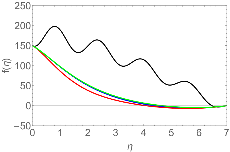
Figure 1: The shape functions of the velocity component $u$ as the function of $\eta$ for various physical parameter sets. The integration parameters are the same for all four functions $f(0)=150,f(7)=0,f^{\prime}(0)=-40,f^{\prime}(7)=10$ which model a flow in a finite duct. The velocity is maximal at one boundary and zero at the other. The acceleration is negative on the maximal velocity side and positive on the other. The constants $G$ and $e$ are set to unity and $a=0.5$ The black curve is for a parameter set of $\kappa=4.1,\nu=3.4,c=33$. Notice the heavy oscillations. The blue, red and green curves represent results for $c=0$ with $\kappa=\nu=3.1$ , $\kappa=0.8<\nu=4.1,$ and $\kappa=5.2>\nu=1.8,$ respectively.

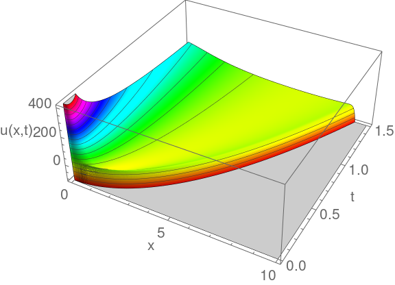
Figure 2: The velocity distribution functions $u(x,t)$. The parameters are $c=0,a=0.5,\kappa=0.8$ and $\nu=4.1$.

Figure 3: The shape function of the temperature Eq. (7) as the function of $\eta$. The parameters are the same as at Fig. 2.

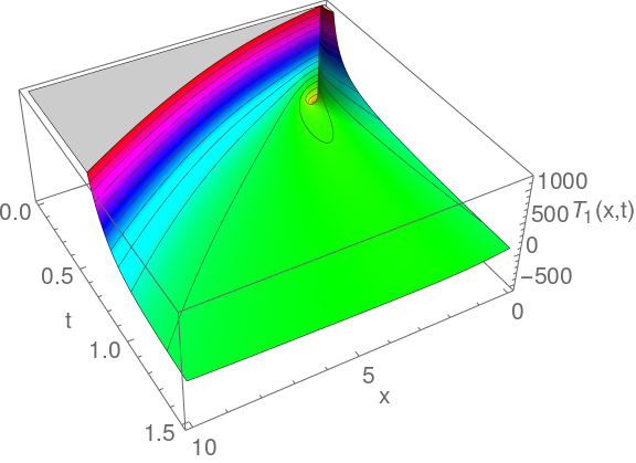
Figure 4: The projected temperature distribution function $T_{1}(x,t)$. The parameters are the same as at Fig. 2.

Figure 5: The shape function of pressure field Eq. (9) as the function of $\eta$. The parameters are same as at Fig. 2.

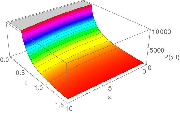
Figure 6: The projected pressure distribution function $P(x,t)$. The parameters are same as at Fig. 2.

3 Summary and Outlook

We gave a physically reasonable generalization of the classical OB equation which was the first study in the paradigm of chaos. As a new feature we added an additional source term to the heat conduction equation, which is proportional to the square of the velocity gradient and called viscous heating. Instead of the usual Galerkin method which applies truncated Fourier series we took the two-dimensional generalization of the self-similar Ansatz and found a coupled non-linear ODE system which can be solved with quadrature.

To our best knowledge certain parts of the climate models are based on the OB equations therefore our results might give an interesting contribution to such studies.

4 Acknowledgment

This work was supported by Project no. 129257 implemented with the support provided from the National Research, Development and Innovation Fund of Hungary, financed under the OTKA 2018 funding scheme. The ELI-ALPS project (GINOP-2.3.6-15-2015-00001) is supported by the European Union and co-financed by the European Regional Development Fund.

References

- [1] M.J. Boussinesq, Comptes Rendus Acad. Sci (Paris), 72, 755 (1871).
- [2] A. Oberbeck, Annal. der Phys. und Chemie Neue Feralolge 7, 271 (1879).
- [3] B. Saltzman, J. Atmos. Sci. 19, 329 (1962).
- [4] E.N. Lorenz, J. Atmos. Sci. 20, 130 (1963).
- [5] J. Gleick, Chaos, Making a new science, Viking Penguin Inc., 1986.
- [6] I.F. Barna, M. László, Chaos, Solitons and Fractals 78, 249 (2015).
- [7] I.F. Barna, M.A. Pocsai, S. Lökös and L. Mátyás Chaos, Solitons and Fractals 103, 336 (2017).
- [8] E. L. Koschmieder, Bènard Cells and Taylor Vortices, Cambridge 1993.
- [9] A. V. Getling, Rayleigh - Bènard Convection: Structures and Dynamics, World Scientific 1998.
- [10] R. Kh. Zeytounian, Convection in Fluids: A Rational Analysis and Asymptotic Modelling, Springer 2009.
- [11] D. Goluskin, Internally Heated Convection and Rayleigh - Bènard Convection , Springer 2016.
- [12] E.S.C. Ching, Statistics and Scaling in Turbulent Rayleigh - Bènard Convection, Springer 2014.
- [13] W. van Saarloos, Phys. Rep., 386, 29 (2003).
- [14] M. Cross and H. Greenside, Pattern Formation and Dynamics in Nonequilibrium Systems, Cambridge University Press 2009.
- [15] R. Meyer-Spasche, Pattern Formation in Viscous Flow, Springer, 1991.
- [16] H. Aref, J.R. Blake, M. Budisić, et al. Rev. Mod. Phys., 89, 025007 (2017).
- [17] Z. Toroczkai, Gy. Károlyi, Á. Péntek, T. Tél and C. Grebogi, Phys. Rev. Lett. 80, 500 (1998).
- [18] S. Boccaletti, C. Grebogi, Y.C. Lai, H. Mancini and D. Maza, Phys. Rep., 329, 103 (2000).
- [19] A. J. Harfash and G. A. Meften, Chaos, Solitons and Fractals 107, 18 (2018).
- [20] W. Khan and F. Yousafzai, Advanced Trends in Mathematics 1, 27 (2014).
- [21] T. Akinaga, T. Itano and S. Generalis, Chaos, Solitons and Fractals 91, 533 (2016).
- [22] S. R. de Groot and P. Mazur, Non-Equilibrium Thermodynamics, Dover Publications, Inc, New York, 1984.
- [23] L. Mátyás, T. Tél and J. Vollmer, Phys. Rev. E, 64, 056106 (2001).
- [24] K.M. Saad, A. Atangana and D. Baleanu, Chaos 28, 063109 (2018).
- [25] T. Tél, J. Vollmer and L. Mátyás, Europhys. Lett. 53, 458 (2001).
- [26] S. E. Ivanov and V. G. Melnikov, International Journal of Mathematical Analysis 9, 2659 (2015).
- [27] G. Bognár and K. Hriczó, Acta Polytechnica Hungarica 8, 131 (2011).
- [28] G. Bognár and K. Hriczó, Recent Advances in Fluid Mechanics, Heat and Mass Transfer, Page 198 Published by WSEAS Press (2012).
- [29] P.A. Madsen and D.R. Furman, B. Wang, Coastal Engineering 53, 487 (2006).
- [30] A.-M. Wazwaz, Journal of Computational and Applied Mathematics 207, 18 (2007).
- [31] A.-M. Wazwaz, Communication in Nonlinear Science and Numerical Simulation 13, 889 (2008).
- [32] F. Shi, J.T. Kirbi, J.C. Harris, J.D. Geiman and S.T. Grilli, Ocean Modelling 43, 36 (2012).
- [33] V. Roeber and K.F. Cheung, Coastal Engineering 70, 1 (2012).
- [34] A.-M. Wazwaz, Ocean Engineering 53, 1 (2012).
- [35] M. A. Helal, A. R. Seadawy and M. H. Zekry, Applied Mathematics and Computation 232, 1094 (2014).
- [36] X.-J. Yang, T. Machado and D. Baleanu, Fractals 25, 1740006 (2017).
- [37] M. Kazolea and A.I. Delis, European Journal of Mechanics / B Fluids 72, 432 (2018).
- [38] N. Kolkovska and M. Dimova, Cent. Eur. J. Math 10, 1159 (2012).
- [39] R. Danchin and M. Paicu, Commun. Math. Phys. 290, 1 (2009).
- [40] T. Gastine, J. Wicht and J.M. Aurnou, Journal of Fluid Mechanics 778, 721 (2015).
- [41] I.L. Animasaun, Ain Shams Engineering Journal 7, 755 (2016).
- [42] S. Weiss, X. He, G. Ahlers, E. Bodenschatz and O. Shishkina, Journal of Fluid Mechanics 851, 374 (2018).
- [43] M. Lappa and T. Gradinscak, International Journal of Heat and Mass Transfer 121, 412 (2018).
- [44] H.-D. Xi, Q. Zhou, and K.-Q. Xia, Physical Review E 73, 056312 (2006).
- [45] G. Ahlers, X. He, D. Funfschilling and D. Bodenschatz, New Journal of Physics 14, 103012 (2012).
- [46] G. Ahlers, E. Bodenschatz and X. He, Journal of Fluid Mechanics 758, 436 (2014).
- [47] A. Parodi, K.A. Emanuel and A. Provenzale, New Journal of Physics 5, 106 (2003).
- [48] I.F. Barna and L. Mátyás, Miskolc Mathematical Notes 14, 485 (2013).
- [49] I.F. Barna and L. Mátyás, Fluid Dynamics Research 46, 055508 (2014).
- [50] M. Yuen, Communications in Nonlinear Science and Numerical Simulation 20, 634 (2015).
- [51] Y. Chen, E. Fan and M. Yuen, Applied Mathematics Letters 67, 46 (2017).
- [52] M. Gugat and S. Ulbrich, Journal of Mathematical Analysis and Applications 454, 439 (2017).
- [53] J.P. Vishwakarma , G. Nath and R.K. Srivastava, Ain Shams Engineering Journal 9, 1717 (2018).
- [54] I.L. Animasaun and I. Pop, Alexandria Engineering Journal 56, 647 (2017).
- [55] I.F. Barna Self-Similar Analysis of Various Navier-Stokes Equations in Two or Three Dimensions in Handbook on Navier-Stokes Equations, Theory and Applied Analysis edited by D. Campos, Nova Publishers, New York, 2017.
- [56] K. Hooman and A. Ejlali, Int. Comm. Heat and Mass Trasf. 37, 34 (2010).
- [57] T. Zhang, L. Jia, L. Yiang and Jaluria, Int. Comm. Heat and Mass Trasf. 53, 49272 (2010).
- [58] T.M. Squires and S.R. Quake, Rev. Mod. Phys. 77, 977 (2005).
- [59] G.L. Morini, Viscous Heating in Encyklopedia of Microfluidics and Nanofluidics edited by D. Li, Springer, 2014.
- [60] H.Gad-el-Hak, The Microelectromechanical systems (MEMS) Handbook, Taylor and Francis, 2006.
- [61] M.G. Haines, P.D. LePell, C.A. Coverdale, B. Jones, C. Deeney and J.P. Apruzese, Phys. Rev. Lett. 96, 075003 (2006).
- [62] A. Costa and G. Macedonio, Nonlin. Proc. Geophys., 10, 545 (2003).
- [63] J. Li, arXiv:1801.09395v2 [math.AP].
- [64] L. Sedov, Similarity and Dimensional Methods in Mechanics CRC Press 1993.
- [65] I.F. Barna and R. Kersner, J. Phys. A: Math. Theor. 43, 375210 (2010).
- [66] I.F. Barna and R. Kersner, Adv. Studies Theor. Phys. 5, 193 (2011).
- [67] H. Schlichting and K. Gersten, Boundary-Layer Theory, Springer 2017.
- [68] M. Benlahsen, M. Guedda and R. Kersner, Math. Comput. Modelling 47, 1063 (2008).