Adversarial Defense Framework for Graph Neural Network

Abstract

Graph neural network (GNN), as a powerful representation learning model on graph data, attracts much attention across various disciplines. However, recent studies show that GNN is vulnerable to adversarial attacks. How to make GNN more robust? What are the key vulnerabilities in GNN? How to address the vulnerabilities and defense GNN against the adversarial attacks? In this paper, we propose DefNet, an effective adversarial defense framework for GNNs. In particular, we first investigate the latent vulnerabilities in every layer of GNNs and propose corresponding strategies including dual-stage aggregation and bottleneck perceptron. Then, to cope with the scarcity of training data, we propose an adversarial contrastive learning method to train the GNN in a conditional GAN manner by leveraging the high-level graph representation. Extensive experiments on three public datasets demonstrate the effectiveness of DefNet in improving the robustness of popular GNN variants, such as Graph Convolutional Network and GraphSAGE, under various types of adversarial attacks.

1 Introduction

Graph Neural Network (GNN) has received wide attention Defferrard et al. (2016); Hamilton et al. (2017a); Velickovic et al. (2017); Kipf and Welling (2016); Li et al. (2015); Gilmer et al. (2017) in the past few years. It extends the traditional neural networks for processing the data represented in the graph domains including social networks, protein-protein interaction network, information network, and et al. The goal of GNN is to learn the representation of the graph, in the node level or graph level, via a neural network consisting of a neural encoding function and a decoding function. Because of its remarkable graph representation learning ability, GNN has been explored in various real-world applications, such as physics system Battaglia et al. (2016), financial system Liu et al. (2018), protein interface prediction Fout et al. (2017), and disease classification Rhee et al. (2018).

However, recent studies Dai et al. (2018); Zugner et al. (2018) have found that GNNs can easily be compromised by adversarial attacks. These adversarial attacks are often stealthy and only require small perturbations (e.g., by adding or dropping edges) of the graph structure and/or node features to induce the GNNs to make incorrect predictions for some specific nodes with high confidence. This makes it highly risky for those aforementioned domains that GNN applied, especially security or financial applications, because it could potentially open the backdoor for the attackers.

Despite recent advances in adversarial attacks Dai et al. (2018); Zugner et al. (2018); Goodfellow et al. (2015), the question of how to defend the GNN against the adversarial attacks has not been satisfyingly addressed yet. Nonetheless, some works have been proposed to improve the robustness of traditional Deep Neural Networks (DNNs) Goodfellow et al. (2015); Madry et al. (2017); Na et al. (2017); Samangouei et al. (2018); Papernot et al. (2016); Jia and Liang (2017). Among them, adversarial learning, which augments the training data with adversarial examples during the training stage Goodfellow et al. (2015); Madry et al. (2017); Na et al. (2017), has shown to be most effective in defending the powerful adversarial attacks Athalye et al. (2018). However, these defense works only focus on either image data Samangouei et al. (2018) or text data Jia and Liang (2017). When it comes to adversarial defense in graph data, where the graph structure and the nodes’ feature are often discrete, there is no existing work. It is difficult to defend the GNN against the adversarial attacks due to two major challenges: (1) the latent vulnerabilities from every layer of GNN and (2) the discrete adversarial space.

Naturally, the vulnerabilities of GNN can come from every layer of its unique architecture: the aggregation layer and the perceptron layer. As the main strength of GNN, the aggregation layer computes the node representation by leveraging its context, which covers the graph structure. However, the aggregation layer can also be vulnerable due to the effect that, the node representation depends not only on its own feature but also on its neighborhood Kipf and Welling (2016). Zugner et al. (2018) has shown that the attack can be conducted without touching of the target node, since the attack happening on the other neighbors may propagate to the nodes that are not attacked. Another vulnerability is related to the input dimension, which inherits from DNNs. As shown in Simon-Gabriel et al. (2018), there is a one-to-one relationship between the adversarial vulnerability and the input dimension, such that the adversarial vulnerability increases with the input dimension.

In addition to the lack of understanding of the vulnerabilities, the discrete adversarial space is also an issue. Different from images where the data are continuous, the graphs are discrete and the combinatorial nature of the graph structures makes it much more difficult than the text data. Thus, how to generate good adversarial graph samples to augment the training data for GNN is a non-trivial problem. Simply generating adversarial samples from a noise distribution will not tailor toward the graph data. And the generated ineffectual adversarial samples could even weaken the robustness of the model against various adversarial attacks.

To tackle the aforementioned two challenges, in this paper, we propose DefNet, an effective framework for defending popular Graph Neural Networks against adversarial attacks. DefNet consists of two modules: GER (Graph Encoder Refining) and ACL (Adversarial Contrastive Learning). First, GER investigates the vulnerabilities in the aggregation layer and the perceptron layer of a GNN encoder, and applies dual-stage aggregation and bottleneck perceptron to address those vulnerabilities. Then, in ACL module, the GNN is trained in an adversarial contrastive learning style. To overcome the discrete adversarial space problem, ACL models the adversarial learning as a conditional GAN by leveraging the high-level graph representation as auxiliary information to regularize the node representation learning. To evaluate the performance of DefNet, we perform an extensive set of experiments on three public graph datasets. The results demonstrate the effectiveness of our proposed framework on defending the popular GNN variants, such as Graph Convolutional Network and GraphSAGE, against various types of adversarial attacks.

2 Preliminaries and Problem Formulation

In this paper, we use bold lowercase for vectors (e.g., $\mathbf{a}$), bold capital for matrices (e.g., $\mathbf{A}$), and calligraphic letters for sets (e.g., $\mathcal{A}$). A graph is represented by a triplet $G=(\mathcal{V},\mathcal{E},\mathbf{X})$, where $\mathcal{V}=\{v_{1},...,v_{n}\}$ is the set of nodes, $\mathcal{E}\subseteq\mathcal{V}\times\mathcal{V}$ is the set of edges, and $\mathbf{X}\in\mathbb{R}^{n\times d}$ is a matrix with the $v$-th row, $\mathbf{x}_{v}$, representing the $d$-dimensional feature vector of node $v$. Also, $|\mathcal{V}|=n$ and $|\mathcal{E}|=m$ are the number of nodes and edges in $G$, respectively. Following the existing work on adversarial attacks Zugner et al. (2018), in this paper, we consider graphs that are undirected and attributed.

A Graph Neural Network (GNN) is a function $f_{GNN}$, parameterized by neural networks. Typically, $f_{GNN}$ is composed of an encoding function $ENC(\cdot)$ and a decoding function $DEC(\cdot)$, such that $f_{GNN}(G)\equiv DEC(ENC(G))$. In particular, we have

$$\mathbf{h}_{v} =ENC(\mathbf{x}_{v},\{\mathbf{x}_{u}\}_{u\in\mathcal{N}_{v}})$$ (1)

$$\mathbf{o}_{v} =DEC(\mathbf{h}_{v})$$ (2)

where $\mathbf{h}_{v}$ is the embedding vector of node $v$, $\mathbf{o}_{v}$ is the decoded output, and $\mathcal{N}_{v}$ is the set of neighboring nodes of $v$ in graph $G$, i.e., $\mathcal{N}_{v}=\{u|(u,v)\in\mathcal{E},(v,u)\in\mathcal{E}\}$.

The encoding function is characterized by an aggregation layer and a perceptron layer Hamilton et al. (2017b). The aggregation layer aims to aggregate the neighborhood information of a node for updating its embedding, which encourages message propagation along the graph. Formally, the aggregation function is defined as follows:

$$\mathbf{a}_{v}^{(k)} =AGG(\{\mathbf{h}_{u}^{(k-1)}\}_{u\in\mathcal{N}_{v}})$$ (3)

where $\mathbf{a}_{v}^{(k)}$ is the aggregated representation of the neighboring embeddings $\mathbf{h}_{u}^{(k-1)}$ (at the ($k-1$)-th layer) of node $v$.

After obtaining $\mathbf{a}_{v}^{(k)}$, the perceptron layer transforms it to a hidden nonlinear space to reach an updated embedding, $\mathbf{h}_{v}^{(k)}$, of node $v$ by performing:

$$\mathbf{h}_{v}^{(k)}=PERCE(\mathbf{a}_{v}^{(k)})$$ (4)

Depending on different tasks, the parameters of $f_{GNN}$ can be trained in a supervised or unsupervised manner. For example, considering node classification, each node $v$ has a label $y_{v}\in\mathcal{Y}=\{1,2,...,Y\}$. Then, the loss function can be defined using the decoding function $DEC(\cdot)$ and Softmax:

$$\ell=\frac{1}{N}\sum_{v\in\mathcal{V}}\text{Softmax}(DEC(\mathbf{h}_{v}),y_{v})$$ (5)

In an unsupervised scenario, a cross-entropy loss can be used to encourage similarities between nearby nodes and difference between disparate nodes Hamilton et al. (2017a):

$$\ell=\log(\sigma(\mathbf{h}_{u}^{T}\mathbf{h}_{v}))+\sum_{n=1}^{K}\mathbb{E}_{v_{n}\sim P_{n}(v)}\log(\sigma(-\mathbf{h}_{v_{n}}^{T}\mathbf{h}_{v}))$$ (6)

where $u\in\mathcal{N}_{v}$ is a neighbor of $v$, $P_{n(v)}$ is the noise distribution for negative sampling, $K$ is the number of negative samples, and $\sigma$ denotes the sigmoid function.

Problem Statement. Suppose we have a graph $G=(\mathcal{V},\mathcal{E},\mathbf{X})$ and a well-trained $f_{GNN}$ on $G$. In the testing phase, $f_{GNN}$ is expected to perform good predictions on $G$ (e.g., transductive classification) and on other graphs with a similar distribution of $G$ (e.g., inductive classification). The goal of an adversarial attack is to maliciously transform $G$ to a perturbed graph $G^{\prime}=(\mathcal{V}^{\prime},\mathcal{E}^{\prime},\mathbf{X}^{\prime})=P(G)$, such that the performance of the original model $f_{GNN}$ on the perturbed graph $G^{\prime}$ drops dramatically.

In this work, we study the problem of adversarial defense for GNN, that is to defend a GNN against the adversarial attacks. More formally, given a graph $G$, our goal is to build a robust GNN framework $f_{GNN}^{(robust)}$ during the training phase, such that in the testing phase, the robust model preserves its good performance on the attacked $G^{\prime}$.

3 The DefNet Framework

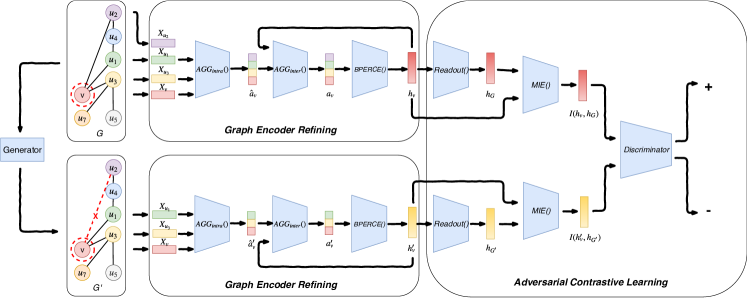
Figure 1: An overview of DefNet framework. DefNet contains two modules: Graph Encoder Refining (GER) and Adversarial Contrastive Learning (ACL). The GER module polishes the encoder of GNN with mean intra-layer aggregation (i.e., AGG${}_{intra}()$), dense-connected inter-layer aggregation (i.e., AGG${}_{inter}()$) and bottleneck perceptron (i.e., BPERCE()). The ACL module takes the benign graph samples (e.g., $G$) and the adversarial graph samples (e.g., $G^{\prime}$) as the input to train the refined GNN in a conditional GAN manner.

To address the two key challenges introduced in Section 1, we propose an adversarial defense framework DefNet with two modules: Graph Encoder Refining (GER) and Adversarial Contrastive Learning (ACL) as illustrated in Fig. 1. In GER module, we aim to examine the vulnerabilities in every layer of a GNN encoder, and propose corresponding strategies to address these vulnerabilities. And in ACL module, our goal is to train the GNN to be more distinguishable between real benign samples and adversarial samples.

3.1 GER: Graph Encoder Refining

3.1.1 Dual-Stage Aggregation

As the first layer of GNN, the aggregation layer leverages the graph structure (i.e., the local context of each node) to improve the GNN performance by aggregating neighbourhood. However, due to graph properties such as homophily London and Getoor (2014), the representation of a single node can easily be affected by its local context. Consequently, attackers can compromise a node’s prediction without directly changing its features and/or edges Zugner et al. (2018).

To improve the robustness of the aggregation layer, we propose a dual-stage aggregator. As shown in the middle of Fig. 1, in the first stage, an intra-layer aggregation integrates the neighbourhood in a mean pooling manner. In the second stage, an inter-layer aggregation combines the node representations from multiple layers in a dense-connection manner.

The intra-layer aggregation aims to compute the new representation of a node by aggregating its local neighbourhood spatially. Typical neighbourhood aggregation operation includes sum Xu et al. (2018), max Hamilton et al. (2017a), and mean Kipf and Welling (2016). The sum aggregator sums up the features within the neighbourhood $\mathcal{N}_{v}$, which captures the full neighbourhood. The max aggregator generates the aggregated representation by element-wise max-pooling. It captures neither the exact structure nor the distribution of the neighbourhood $\mathcal{N}_{v}$. The mean aggregator averages individual element features out. Different from the sum and max aggregators, it can capture the distribution of the features in the neighbourhood $\mathcal{N}_{v}$.

The adversarial attacks are usually stealthy and can only perform small-scale modifications to the graph data. An ideal aggregator should be robust to such subtle perturbations. Among the three aggregators, the max aggregator is very sensitive to the distinct modification (e.g., by adding a new neighbor of a different class with a big value), even though it is very small. For the sum aggregator, it can also be affected by this kind of modification. In contrast, the mean aggregator is less sensitive to the small-scale modification and thus is more robust to adversarial attacks.

Therefore, in our GER module, the intra-layer aggregation $AGG_{intra}()$ aggregates the neighborhood in a mean pooling manner. Formally, it is defined as follows:

$$\hat{\mathbf{a}}_{v}^{(k)} =AGG_{intra}(\{\mathbf{h}_{u}^{(k-1)}:u\in\mathcal{N}_{v}\}))$$ (7)

$$=\frac{1}{|\mathcal{N}_{v}|}\sum_{u\in\mathcal{N}_{v}}\mathbf{h}_{u}^{(k-1)}$$ (8)

where $k$ is the index of layer/iteration, $|\mathcal{N}_{v}|$ is the cardinality of the neighborhood of node $v$, and $\hat{\mathbf{a}}_{v}^{(k)}$ is the result of the intra-layer aggregation.

In the second stage, the layer-wise aggregation is employed to connect current layer of the network to its previous layers, such that more structural information can be covered. Recently, GNNs, such as GCN and GraphSAGE, leverage the skip-connection to aggregate the representation from the predecessor layer and drop the rest of intermediate representations during the information propagation within $k$-hop neighbors. However, stacking multiple such layers could also propagate the noisy or adversarial information from an exponentially increasing number of expanded neighborhood member Kipf and Welling (2016).

To address this problem, we propose a dense-connected inter-layer aggregation, as inspired by the DenseNet Huang et al. (2017). Our method keeps all intermediate representations and aggregates them together to compute the recent-layer representation. In this way, the recent layer is connected with all previous hidden layers, allowing the subsequent layer to selectively but adaptively aggregate structure information from different hops. Consequently, the robustness can be improved for deep GNN.

Formally, the dense-connected inter-layer aggregation $AGG_{inter}()$ is constructed as follows:

$$\mathbf{a}_{v}^{(k)} =AGG_{inter}(\hat{\mathbf{a}}_{v}^{k},\mathbf{h}_{v}^{(k-1)},\mathbf{h}_{v}^{(k-2)}...\mathbf{h}_{v}^{(1)})$$ (9)

$$=[\hat{\mathbf{a}}_{v}^{k};\mathbf{h}_{v}^{(k-1)};\mathbf{h}_{v}^{(k-2)};...;\mathbf{h}_{v}^{(1)}]$$ (10)

where $[\cdot;\cdot]$ represents the feature concatenation operation.

3.1.2 Bottleneck Perceptron

In this section, we propose the bottleneck perceptron for mapping the aggregated representation to node embedding in a non-linearly low-dimensional space. Particularly, it consists of a bottleneck mapping followed by a nonlinear mapping.

Recent researches have empirically studied the one-to-one relationship between the adversarial vulnerability and the input dimensionality, and theoretically proved that the adversarial vulnerability of neural networks deteriorates as the input dimensionality increases Simon-Gabriel et al. (2018). On the other hand, it is common that real data are not truly high-dimensional Levina and Bickel (2005). The data in a high-dimensional space can be well embedded into a lower dimensional space for both better effectiveness and efficiency. Therefore, it is important to perform dimensionality reduction on the input to improve the robustness of a GNN .

To this purpose, we design a bottleneck mapping, such that the output dimensionality is much lower than that of the input. Meanwhile, we add a nonlinear gating function to capture the nonlinearity of the data. In particular, we use rectified linear unit (ReLU) as the activation function. Formally, the bottleneck perceptron is defined as follows:

$$\mathbf{h}_{v}^{(k)}=BPERCE(\mathbf{a}_{v}^{(k)})=RELU((\mathbf{W}^{(k)}_{p})\mathbf{a}_{v}^{(k)})$$ (11)

where $\mathbf{W}^{(k)}_{p}$ is the trainable mapping matrix. The output of this module is the low-dimensional node embedding.

3.2 ACL: Adversarial Contrastive Learning

After addressing the vulnerabilities of the graph encoder, the GNN may still be vulnerable to the adversarial attacks due to the scarcity of training data Pinto et al. (2017). To handle this issue, in this section, we introduce the adversarial contrastive learning to regularize the training of the GNN.

Contrastive learning has been widely found useful for representation learning of graph data Hamilton et al. (2017b). Its objective is written by:

$$L =\mathbb{E}_{(x^{+},y^{+},y^{-})}[\ell_{\mathbf{w}}(x^{+},y^{+},y^{-})]$$ (12)

where $\ell_{\mathbf{w}}(x^{+},y^{+},y^{-})$ scores a positive tuple $(x^{+},y^{+})$ against a negative one $(x^{+},y^{-})$, and $\mathbb{E}_{(x^{+},y^{+},y^{-})}$ represents the expectation w.r.t. the joint distribution over the positive and negative samples. Since negative sampling is independent of the positive label, Eq. 12 can be rewritten by:

$$L =\mathbb{E}_{p(x^{+})}\mathbb{E}_{p(y^{+}|x^{+})p(y^{-}|x^{+})}[\ell_{\mathbf{w}}(x^{+},y^{+},y^{-})]$$ (13)

$$=\mathbb{E}_{p(x^{+})}[\mathbb{E}_{p^{+}(y|x)}D_{\mathbf{w}}(x,y)-\mathbb{E}_{p^{-}(y|x)}D_{\mathbf{w}}(x,y)]$$ (14)

where $D_{\mathbf{w}}(x,y)$ measures the correlation between $x$ and $y$.

Traditional graph embedding methods adopt a noise contrastive estimation approach and approximate $p(y^{-}|x^{+})$ with a noise distribution probability $p_{n}(y)$, such that

$$L =\mathbb{E}_{p(x^{+})}[\mathbb{E}_{p(y^{+}|x^{+})p_{n}}[\ell_{\mathbf{w}}(x^{+},y^{+},y^{-})]]$$ (15)

$$=\mathbb{E}_{p(x^{+})}[\mathbb{E}_{p^{+}(y|x)}D_{\mathbf{w}}(x,y)-\mathbb{E}_{p_{n}}D_{\mathbf{w}}(x,y)]$$ (16)

However, using $p_{n}$ sacrifices the performance of learning as the negative samples are produced based on a noise distribution. What is worse, using $p_{n}$ also harms the robustness of the learning as the negative samples are produced without considering the adversarial samples.

To address this problem, we model the negative sampler by a generator under a conditional distribution $g_{\theta}(y|x)$. Formally, it is defined as follows:

$$L =\mathbb{E}_{p(x^{+})}[\mathbb{E}_{p^{+}(y|x)}D_{\mathbf{w}}(x,y)-\mathbb{E}_{g_{\theta}(y|x)}D_{\mathbf{w}}(x,y)].$$ (17)

We optimize the above objective function in a minimax adversarial learning manner as follows:

$$\min_{G_{\theta}}\max_{D_{\mathbf{w}}}\{\mathbb{E}_{p^{+}(y|x)}[\log D_{\mathbf{w}}(x,y)]+\mathbb{E}_{g_{\theta}(x,y)}[\log(1-D_{\mathbf{w}}(G_{\theta}(x,y)))]\}.$$ (18)

This formulation is closely related to GAN by regarding $D_{\mathbf{w}}$ as the discriminator and $G_{\theta}$ as the generator. The generative model $G_{\theta}$ captures the data distribution, and the discriminative model $D_{\mathbf{w}}$ estimates the probability that a sample comes from the training data rather than $G_{\theta}$. $G_{\theta}$ and $D_{\mathbf{w}}$ are trained jointly: we adjust the parameters of $G_{\theta}$ to minimize $\log(1-D_{\mathbf{w}}(G_{\theta}(x,y)))$ and adjust the parameters of $D_{\mathbf{w}}$ to minimize $\log D_{\mathbf{w}}(x,y)$, as if they follow the two-player minimax game.

However, the vanilla GAN does not take any constraint into account for the generator, and the generator is not tailored to the graph data. This may cause suboptimal quality of the generated adversarial samples since the adversarial latent space can not be effectively explored. This limitation may reduce the performance of the feature learning. To overcome it, we adopt a conditional GAN configuration, which extends a conditional model where the generator and discriminator are both conditioned on some extra information. The extra information could be any kind of auxiliary information, such as class labels or data from other modalities.

The condition can be realized by feeding extra information into both the discriminator and generator as an additional input layer. As shown in Fig. 1, we consider the high-level graph representation (e.g., graph embedding $\mathbf{h}_{G}$) as a global constraint to regularize the node representation learning. The motivation is based on the observation Dai et al. (2018) that global level representation such as graph embedding is less sensitive to the adversarial perturbation than the local-level representation such as node embedding. Thus, the global graph representation can be used to guide the robust learning of the local node representations. Accordingly, the objective of our adversarial contrastive learning becomes:

$$\min_{G}\max_{D}\{\mathbb{E}_{p^{+}}[\log D_{\mathbf{w}}(\mathbf{h}_{v}|\mathbf{h}_{G})]\\ +\mathbb{E}_{g_{\theta}}[\log(1-D_{\mathbf{w}}(G_{\theta}(\mathbf{h}^{\prime}_{v}|\mathbf{h}_{G}))))]\}$$ (19)

where $\mathbf{h}^{\prime}_{v}$ is the node embedding from the generated adversarial samples $G^{\prime}=(V^{\prime},E^{\prime},X^{\prime})=P(G)$. Here, the perturbation function $P(\cdot)$ can be defined similarly to Zugner et al. (2018).

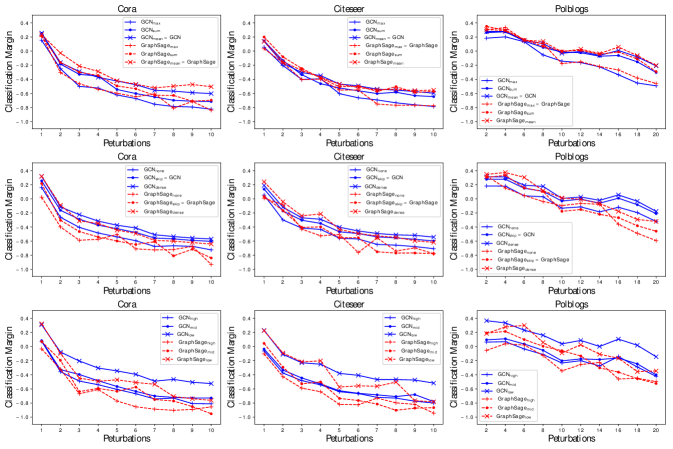
Figure 2: Evaluation of the GER.

To obtain the graph embedding, we employ a $READOUT$ function. Given the node representations $\{h_{v}\}_{v\in\mathcal{V}}$ of graph $G$, the $READOUT$ function performs a mean pooling followed by a nonlinear mapping as follows:

$$\mathbf{h}_{G} =READOUT({\mathbf{h}_{v}^{(k)}|v\in\mathcal{V}})$$ (20)

$$=\sigma(\mathbf{W}_{r}(\frac{1}{N}\sum_{i=1}^{N}\mathbf{h}_{i}^{K})))$$ (21)

where $\sigma$ represents the sigmoid function, $\mathbf{W}_{r}$ represents a trainable linear mapping matrix, and $K$ denotes the total number of layers/iterations. This module follows the idea of using the pooling function to compute the high-level global representation in CNN. The reason of using a mean pooling is similar to that of neighborhood aggregation, i.e., the representation generated by the mean operation is more stable and less sensitive to the small-scale adversarial attacks.

For the discriminator, we employ a mutual information estimator to jointly model the local and global graph representations via a bilinear scoring function:

$$\vspace{-5pt}D_{\mathbf{w}}(\mathbf{h}_{v}|\mathbf{h}_{G}) =I(\mathbf{h}_{v},\mathbf{h}_{G})=\sigma(\mathbf{h}_{v}\mathbf{W}_{D}\mathbf{h}_{G})\vspace{-5pt}$$ (22)

where $I(\mathbf{h}_{v},\mathbf{h}_{G})$ represents the mutual information between the node embedding and graph embedding. $\mathbf{W}_{D}$ is a trainable scoring matrix and $\sigma$ denotes the sigmoid function.

4 Experiments

In this section, we evaluate our proposed DefNet framework on defending adversarial attacks.

4.1 Datasets

Table 1: The statistics of the datasets.

Dataset	#Node	#Edge	#Feature	#Class
Cora	2,810	7,981	1,433 (Categorical)	7
Citeseer	2,110	3,757	3,703 (Categorical)	3
PolBlogs	1,222	16,714	Identity feature	2

We use three benchmark datasets including two academic networks (Cora and Citeseer) and a social network (PolBlogs) for node classification tasks. Table 1 shows the statistics of these datasets. We select the largest connected components in each dataset for our experiments, and we split all the datasets randomly into a labeled set (80%) and an unlabeled set (20%). We then further divide the labeled set into a training set (50%) and a validate set (50%).

4.2 Experiment Setup

4.2.1 Attack Models

We conduct three types of popular adversarial attacks:

• RAND (a random perturbation attack): Given the target node, it randomly adds edges to the node that belongs to a different class and/or deletes an edge that connected to the node within the same class.

• FGSM (a gradient based attack) Goodfellow et al. (2015)): It generates adversarial examples based on the sign of gradient.

• NETTACK (a state-of-the-art optimization based attack Zugner et al. (2018)): It generates adversarial perturbations by searching the perturbation space.

The attack procedure is similar to Zugner et al. (2018). We select $200$ nodes as the targets: $50$ correctly classified nodes with high confidence; $50$ correctly classified nodes but with low confidence; and $100$ random nodes.

4.2.2 Comparing Methods

We evaluate our framework DefNet on two most popular GNN variants: GCN Kipf and Welling (2016) and GraphSAGE Hamilton et al. (2017a). To evaluate the GER module, we compare different versions of GCN and GraphSAGE in terms of intra-layer aggregators (XXX_mean, XXX_sum, XXX_max), inter-layer aggregators (XXX_none (without inter-layer aggregator), XXX_skip (skip based), XXX_dense (dense based)), and output dimensions (XXX_low, XXX_mid, XXX_high) as discussed in Section 3. To evaluate the ACL module, we use the refined GNN after GER (RGCN or RGraphSage) as graph encoder, and consider their variants in terms of adversarial learning methods: XXX_NCL (noise contrastive learning) and XXX_ACL (adversarial contrastive learning).

4.2.3 Configuration

We repeat all the experiments over five different splits of labeled/unlabeled nodes to compute the average results. For GNNs used in the experiments, we set the default number of layers as $3$, and the number of perceptron layers as $2$. We also adopt the Adam optimizer with an initial learning rate of $0.01$, and decay the learning rate by $0.5$ for every $50$ epochs.

4.3 Evaluation of GER

In this experiment, we show the vulnerabilities of the GNN in terms of its aggregation and perceptron components. We also demonstrate the effectiveness of GER in addressing these vulnerabilities.

We test the robustness of different methods under the most powerful attack NETTACK with various adversarial perturbations. We use the classification margin score $s$ as the metric for the classifier performance:

$$s=Z^{*}_{v,c^{gt}_{v}}-max_{c\neq c^{gt}_{v}}Z*_{v,c}$$ (23)

where $Z^{*}_{v,c^{gt}_{v}}$ is the predicted probability for the ground-truth label, while $max_{c\neq c^{gt}_{v}}Z*_{v,c}$ is the incorrect prediction probability with the largest confidence. The larger $s$ is, the higher confidence the classifier has in making a correct prediction.

From the experimental results shown in Fig. 2, we can see that the GCN and GraphSAGE with our proposed GER perform better than the original version and the ones using other aggregation or perceptron methods.

Table 2: Performance comparison under various attacks.

Data	Defense	Clean	Attack models
			RAND	FGSM	NETATTACK
Cora	GCN	0.90	0.60	0.03	0.01
	RGCN	0.88	0.73	0.18	0.15
	$\textsc{RGCN}_{NCL}$	0.85	0.80	0.42	0.38
	$\textsc{RGCN}_{ACL}$	0.92	0.85	0.65	0.60
	GraphSage	0.85	0.70	0.18	0.16
	RGraphSage	0.88	0.78	0.25	0.22
	RGraphSageRCL	0.84	0.82	0.48	0.42
	RGraphSageACL	0.88	0.84	0.67	0.60
Citeseer	GCN	0.88	0.60	0.07	0.02
	RGCN	0.90	0.72	0.20	0.16
	$\textsc{RGCN}_{NCL}$	0.86	0.79	0.52	0.45
	$\textsc{RGCN}_{ACL}$	0.90	0.85	0.70	0.65
	GraphSage	0.83	0.70	0.10	0.04
	RGraphSage	0.86	0.80	0.22	0.18
	RGraphSageRCL	0.82	0.82	0.50	0.48
	RGraphSageACL	0.88	0.84	0.68	0.65
Polblogs	GCN	0.93	0.36	0.41	0.06
	RGCN	0.95	0.40	0.50	0.18
	$\textsc{RGCN}_{NCL}$	0.87	0.65	0.58	0.52
	$\textsc{RGCN}_{ACL}$	0.95	0.80	0.74	0.65
	GraphSage	0.86	0.43	0.40	0.14
	RGraphSage	0.90	0.60	0.48	0.20
	RGraphSageRCL	0.82	0.68	0.59	0.55
	RGraphSageACL	0.89	0.78	0.72	0.68

We can also observe that: (1) The mean intra-aggregator outperforms the sum and max ones; (2) The dense inter-aggregator outperforms the case without the inter-aggregator and the skip inter-aggregator; (3) The lower dimension of the perceptron layer beats both the high and medium ones; (4) Comparing GCN with GraphSAGE, the performance of the latter one is less stable but sometimes performs better, due to a max aggregator combined with the random neighbourhood sampling; and (5) It is also worth noticing that PolBlogs is difficult to attack, since the average degree of the node is high.

4.4 Evaluation of ACL Module and DefNet Framework

In this experiment, we show the effectiveness of the proposed ACL module and overall DefNet framework under various attacks. To guarantee the powerfulness of the adversarial attacks, we set the number of the perturbations as: $n_{p}=d_{v}+2$ with $d_{v}$ to be the degree of the target node. We report the fraction of the target nodes that get correctly classified as accuracy. The results in Table 2 show that the proposed ACL method outperforms all the baselines including the traditional training and noise contrastive learning in terms of datasets, GNN variants, and attack models. We also observe that the original GCN and GraphSAGE are both very venerable to the attacks, but after applying our DefNet framework, both of them become way more robust. For example, GCN can achieve an accuracy of $0.90$ without any attack on Cora data, but the performance significantly drops to $0.03$ under the FGSM attack, while RGCN_ACL (i.e., GCN with DefNet) can still achieve an accuracy of $0.65$.

5 Related Work

5.1 Graph Neural Networks

In recent years, representation learning on graph data via Graph Neural Network (GNN) Defferrard et al. (2016); Hamilton et al. (2017a); Kipf and Welling (2016); Velickovic et al. (2017); Li et al. (2015); Gilmer et al. (2017); Xu et al. (2018) has attracted increasing interests. Many GNN variants have been proposed to leverage the graph structure to capture different proprieties. Defferrard et al. (2016); Hamilton et al. (2017a); Kipf and Welling (2016); Li et al. (2015) followed a neighbourhood aggregation scheme. Gilmer et al. (2017) leveraged the structure information via message passing operation. Their success is built on a supervised end-to-end data-driven learning framework, which is vulnerable to adversarial attacks.

5.2 Attack and Defense on GNNs

Recently, a few attempts have been made to study adversarial attacks on GNNs. Dai et al. (2018) proposed a non-target evasion attack on node classification and graph classification. A reinforcement learning method was used to learn the attack policy that applies small-scale modification to the graph structure. Zugner et al. (2018) introduced a poisoning attack on node classification. This work adopted a substitute model attack and formulated the attack problem as a bi-level optimization. Different from Dai et al. (2018), it attacked both the graph structure and node attributes. Furthermore, it considered both direct attacks and influence attacks. However, there is still limited understanding on why GNNs are vulnerable to adversarial attacks and how to defense against the adversarial attacks. This motivates our work.

6 Conclusion

In this paper, we presented DefNet, an adversarial defense framework for improving the robustness of Graph Neural Networks (GNNs) under adversarial attacks. To address the vulnerabilities in the aggregation layer and perceptron layer of GNN, we proposed the dual-stage aggregation and bottleneck perceptron methods. By leveraging the high-level graph representation, we proposed the adversarial contrastive learning technique to train the GNN in a conditional GAN manner. We evaluated the proposed framework using extensive experiments on three public graph datasets. The experimental results convince us of the effectiveness of our framework on defending the popular GNN variants against various types of adversarial attacks.

References

- Athalye et al. (2018) Anish Athalye, Nicholas Carlini, and David Wagner. Obfuscated gradients give a false sense of security: Circumventing defenses to adversarial examples. arXiv preprint arXiv:1802.00420, 2018.
- Battaglia et al. (2016) Peter Battaglia, Razvan Pascanu, Matthew Lai, Danilo Jimenez Rezende, and Koray kavukcuoglu. Interaction networks for learning about objects, relations and physics. In NIPS, pages 4509–4517, 2016.
- Dai et al. (2018) Hanjun Dai, Hui Li, Tian Tian, Xin Huang, Lin Wang, Jun Zhu, and Le Song. Adversarial attack on graph structured data. arXiv preprint arXiv:1806.02371, 2018.
- Defferrard et al. (2016) Michaël Defferrard, Xavier Bresson, and Pierre Vandergheynst. Convolutional neural networks on graphs with fast localized spectral filtering. In NIPS, pages 3844–3852, 2016.
- Fout et al. (2017) Alex Fout, Jonathon Byrd, Basir Shariat, and Asa Ben-Hur. Protein interface prediction using graph convolutional networks. In NIPS, 2017.
- Gilmer et al. (2017) Justin Gilmer, Samuel S Schoenholz, Patrick F Riley, Oriol Vinyals, and George E Dahl. Neural message passing for quantum chemistry. arXiv preprint arXiv:1704.01212, 2017.
- Goodfellow et al. (2015) Ian J Goodfellow, Jonathon Shlens, and Christian Szegedy. Explaining and harnessing adversarial examples. ICLR, 2015.
- Hamilton et al. (2017a) Will Hamilton, Zhitao Ying, and Jure Leskovec. Inductive representation learning on large graphs. In NIPS, pages 1024–1034, 2017.
- Hamilton et al. (2017b) William L Hamilton, Rex Ying, and Jure Leskovec. Representation learning on graphs: Methods and applications. arXiv preprint arXiv:1709.05584, 2017.
- Huang et al. (2017) Gao Huang, Zhuang Liu, Laurens Van Der Maaten, and Kilian Q Weinberger. Densely connected convolutional networks. In CVPR, pages 4700–4708, 2017.
- Jia and Liang (2017) Robin Jia and Percy Liang. Adversarial examples for evaluating reading comprehension systems. arXiv preprint arXiv:1707.07328, 2017.
- Kipf and Welling (2016) Thomas N Kipf and Max Welling. Semi-supervised classification with graph convolutional networks. arXiv preprint arXiv:1609.02907, 2016.
- Levina and Bickel (2005) Elizaveta Levina and Peter J Bickel. Maximum likelihood estimation of intrinsic dimension. In NIPS, pages 777–784, 2005.
- Li et al. (2015) Yujia Li, Daniel Tarlow, Marc Brockschmidt, and Richard Zemel. Gated graph sequence neural networks. arXiv preprint arXiv:1511.05493, 2015.
- Liu et al. (2018) Ziqi Liu, Chaochao Chen, Xinxing Yang, Jun Zhou, Xiaolong Li, and Le Song. Heterogeneous graph neural networks for malicious account detection. In CIKM, pages 2077–2085, 2018.
- London and Getoor (2014) Ben London and Lise Getoor. Collective classification of network data. Data Classification: Algorithms and Applications, 399, 2014.
- Madry et al. (2017) Aleksander Madry, Aleksandar Makelov, Ludwig Schmidt, Dimitris Tsipras, and Adrian Vladu. Towards deep learning models resistant to adversarial attacks. arXiv preprint arXiv:1706.06083, 2017.
- Na et al. (2017) Taesik Na, Jong Hwan Ko, and Saibal Mukhopadhyay. Cascade adversarial machine learning regularized with a unified embedding. arXiv preprint arXiv:1708.02582, 2017.
- Papernot et al. (2016) Nicolas Papernot, Patrick McDaniel, Xi Wu, Somesh Jha, and Ananthram Swami. Distillation as a defense to adversarial perturbations against deep neural networks. In 2016 IEEE Symposium on Security and Privacy (SP), pages 582–597. IEEE, 2016.
- Pinto et al. (2017) Lerrel Pinto, James Davidson, Rahul Sukthankar, and Abhinav Gupta. Robust adversarial reinforcement learning. In Doina Precup and Yee Whye Teh, editors, ICML, volume 70, pages 2817–2826, International Convention Centre, Sydney, Australia, 2017.
- Rhee et al. (2018) Sungmin Rhee, Seokjun Seo, and Sun Kim. Hybrid approach of relation network and localized graph convolutional filtering for breast cancer subtype classification. In IJCAI, pages 3527–3534, 2018.
- Samangouei et al. (2018) Pouya Samangouei, Maya Kabkab, and Rama Chellappa. Defense-gan: Protecting classifiers against adversarial attacks using generative models. arXiv preprint arXiv:1805.06605, 2018.
- Simon-Gabriel et al. (2018) Carl-Johann Simon-Gabriel, Yann Ollivier, Bernhard Schölkopf, Léon Bottou, and David Lopez-Paz. Adversarial vulnerability of neural networks increases with input dimension. arXiv preprint arXiv:1802.01421, 2018.
- Velickovic et al. (2017) Petar Velickovic, Guillem Cucurull, Arantxa Casanova, Adriana Romero, Pietro Liò, and Yoshua Bengio. Graph attention networks. CoRR, abs/1710.10903(2), 2017.
- Xu et al. (2018) Keyulu Xu, Weihua Hu, Jure Leskovec, and Stefanie Jegelka. How powerful are graph neural networks? arXiv preprint arXiv:1810.00826, 2018.
- Zugner et al. (2018) Daniel Zugner, Amir Akbarnejad, and Stephan Gunnemann. Adversarial attacks on neural networks for graph data. In SIGKDD, pages 2847–2856. ACM, 2018.