Stein Point Markov Chain Monte Carlo

Abstract

An important task in machine learning and statistics is the approximation of a probability measure by an empirical measure supported on a discrete point set. Stein Points are a class of algorithms for this task, which proceed by sequentially minimising a Stein discrepancy between the empirical measure and the target and, hence, require the solution of a non-convex optimisation problem to obtain each new point. This paper removes the need to solve this optimisation problem by, instead, selecting each new point based on a Markov chain sample path. This significantly reduces the computational cost of Stein Points and leads to a suite of algorithms that are straightforward to implement. The new algorithms are illustrated on a set of challenging Bayesian inference problems, and rigorous theoretical guarantees of consistency are established.

1 Introduction

The task that we consider in this paper is to approximate a Borel probability measure $P$ on an open and convex set $\mathcal{X}\subseteq\mathbb{R}^{d}$, $d\in\mathbb{N}$, with an empirical measure $\hat{P}$ supported on a discrete point set $\{x_{i}\}_{i=1}^{n}\subset\mathcal{X}$. To limit scope we restrict attention to uniformly-weighted empirical measures; $\hat{P}=\frac{1}{n}\sum_{i=1}^{n}\delta_{x_{i}}$ where $\delta_{x}$ is a Dirac measure on $x$. The quantisation (Graf & Luschgy, 2007) of $P$ by $\hat{P}$ is an important task in computational statistics and machine learning. For example, quantisation facilitates the approximation of integrals $\int_{\mathcal{X}}f\mathrm{d}P$ of measurable functions $f:\mathcal{X}\rightarrow\mathbb{R}$ using cubature rules $f\mapsto\frac{1}{n}\sum_{i=1}^{n}f(x_{i})$. More generally, quantisation underlies a broad spectrum of algorithms for uncertainty quantification that must operate subject to a finite computational budget. Motivated by applications in Bayesian statistics, our focus is on the situation where $P$ admits a density $p$ with respect to the Lebesgue measure on $\mathcal{X}$ but this density can only be evaluated up to an (unknown) normalisation constant. Specifically, we assume that $p=\frac{\tilde{p}}{C}$ where $\tilde{p}$ is an un-normalised density and $C>0$, such that both $\tilde{p}$ and $\nabla\log\tilde{p}$, where $\nabla=(\frac{\partial}{\partial x^{1}},\ldots,\frac{\partial}{\partial x^{d}})$, can be (pointwise) evaluated at finite computational cost.

A popular approach to this task is Markov chain Monte Carlo (MCMC; Robert & Casella, 2004), where the sample path of an ergodic Markov chain with invariant distribution $P$ constitutes a point set $\{x_{i}\}_{i=1}^{n}$. MCMC algorithms exploit a range of techniques to construct Markov transition kernels which leave $P$ invariant, based (in general) on pointwise evaluation of $\tilde{p}$ (Metropolis et al., 1953) or (sometimes) on pointwise evaluation of $\nabla\log\tilde{p}$ and higher-order derivative information (Girolami & Calderhead, 2011). In a favourable situation, the MCMC output will be approximately independent draws from $P$. However, in this case the $\{x_{i}\}_{i=1}^{n}$ will typically not be a low discrepancy point set (Dick & Pillichshammer, 2010) and as such the quantisation of $P$ performed by MCMC will be sub-optimal. In recent years several attempts have been made to deveop improved algorithms for quantisation in the Bayesian statistical context as an alternative to MCMC:

• Minimum Energy Designs (MED) In (Roshan Joseph et al., 2015; Joseph et al., 2018) it was proposed to obtain a point set $\{x_{i}\}_{i=1}^{n}$ by using a numerical optimisation method to approximately minimise an energy functional $\mathcal{E}_{\tilde{p}}(\{x_{i}\}_{i=1}^{n})$ that depends on $P$ only through $\tilde{p}$ rather than through $p$ itself. Though appealing in its simplicity, MED has yet to receive a theoretical treatment that accounts for the imperfect performance of the numerical optimisation method.

• Support Points The method of (Mak & Joseph, 2018) first generates a large MCMC output $\{\tilde{x}_{i}\}_{i=1}^{N}$ and from this a subset $\{x_{i}\}_{i=1}^{n}$ is selected in such a way that a low-discrepancy point set is obtained. (This can be contrasted with classical thinning in which an arithmetic subsequence of the MCMC output is selected.) At present, a theoretical analysis that accounts for the possible poor performance of the MCMC method has not yet been announced.

• Transport Maps and QMC The method of (Parno, 2015) aims to learn a transport map $T:\mathcal{X}\rightarrow\mathcal{X}$ such that the pushforward measure $T_{\#}Q$ corresponds to $P$, where $Q$ is a distribution for which quantisation by a point set $\{\tilde{x}_{i}\}_{i=1}^{n}$ is easily performed, for instance using quasi-Monte Carlo (QMC) (Dick & Pillichshammer, 2010). Then quantisation of $P$ is provided by the point set $\{T(\tilde{x}_{i})\}_{i=1}^{n}$. The flexibility in the construction of a transport map allows several algorithms to be envisaged, but an end-to-end theoretical treatment is not available at present.

• Stein Variational Gradient Descent (SVGD) A popular methodology due to (Liu & Wang, 2016) aims to take an arbitrary initial point set $\{x_{i}^{0}\}_{i=1}^{n}$ and to construct a discrete time dynamical system $x_{i}^{t}=g_{\tilde{p}}(x_{1}^{t-1},\dots,x_{n}^{t-1})$, indexed by time $t$ and dependent on $\tilde{p}$, such that $\lim_{t\rightarrow\infty}\{x_{i}^{t}\}_{i=1}^{n}$ provides a quantisation of $P$. This can be viewed as a discretisation of a particular gradient flow that has $P$ as a fixed point (Liu, 2017). However, a generally applicable theoretical analysis of the SVGD method itself is not available (note that a compactness assumption on $\mathcal{X}$ was required in Liu, 2017). Note also that, unlike the other methods discussed in this section, SVGD does not readily admit an extensible construction; that is, the number $n$ of points must be a priori fixed.

• Stein Points (SP) The authors of (Chen et al., 2018b) proposed to select a point set $\{x_{i}\}_{i=1}^{n}$ that approximately minimises a kernel Stein discrepancy (KSD; Liu et al., 2016; Chwialkowski et al., 2016; Gorham & Mackey, 2017) between the empirical measure and the target $P$. The KSD can be exactly computed with a finite number of pointwise evaluations of $\nabla\log\tilde{p}$ and, for the (non-convex) minimisation, a variety of numerical optimisation methods can be applied. In contrast to the other methods just discussed, SP does admit a end-to-end theoretical treatment when a grid search procedure is used as the numerical optimisation method (Thms. 1 & 2 in Chen et al., 2018b).

An empirical comparison of several of the above methods on a selection of problems arising in computational statistics was presented in (Chen et al., 2018b). The conclusion of that work was that MED and SP provided broadly similar performance-per-computational-cost at the quantisation task, where the performance was measured by the Wasserstein distance to the target and the computational cost was measured by the total number of evaluations of either $\tilde{p}$ or its gradient. In some situations, SVGD provided superior quantisation to MED and SP but this was achieved at a substantially higher computational cost. At the same time, it was observed that all algorithms considered provided improved quantisation compared to MCMC, but at a computational cost that was substantially higher than the corresponding cost of MCMC.

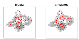
Figure 1: Illustration of Monte Carlo points (MC; left) and Stein Point Markov chain Monte Carlo (SP-MCMC; right) on a Gaussian mixture target $P$. SP-MCMC provides better space-filling properties than MC.

In this paper, we propose Stein Point Markov chain Monte Carlo (SP-MCMC), aiming to provide strong performance at the quantisation task (see Fig. 1) but at substantially reduced computational cost compared to the original SP method. Our contributions are summarised as follows:

• The global optimisation subroutine in SP, whose computational cost was exponential in dimension $d$, is replaced by a form of local search based on MCMC. This allows us to make use of efficient transition kernels for exploration of $\mathcal{X}$, which in turn improves performance in higher dimensions and reduces the overall computational cost.

• Our construction requires a new Markov chain to be initialised each time a point $x_{n}$ is added, however the initial distribution of the chain does not need to coincide with $P$. This enables us to develop an efficient criterion for initialisation of the Markov chains, based on the introduced notion of the “most influential” point in $\{x_{i}\}_{i=1}^{n-1}$, as quantified by KSD. This turns our sequence of local searches into a global-like search, and also leads to automatic “mode hopping” behaviour when $P$ is a multi-modal target.

• The consistency of SP-MCMC is established under a $V$-uniform ergodicity condition on the Markov kernel.

• SP-MCMC is shown, empirically, to outperform MCMC, MED, SVGD and SP when applied to posterior computation in the Bayesian statistical context.

The paper is structured as follows: In Section 2 we review the central notions of Stein’s method and KSD, as well as recalling the original SP method. The novel methodology is presented in Section 3. This is assessed experimentally in Section 4 and theoretically in Section 5. Conclusions are drawn in Section 6.

2 Background

In Section 2.1 we recall the construction of KSD, then in Section 2.2 the SP method of (Chen et al., 2018b), which is based on minimisation of KSD, is discussed.

2.1 Discrepancy and Stein’s Method

A discrepancy is a notion of how well an empirical measure, based on a point set $\{x_{i}\}_{i=1}^{n}\subset\mathcal{X}$, approximates a target $P$. One popular form of discrepancy is the integral probability metric (IPM) (Muller, 1997), which is based on a set $\mathcal{F}$ consisting of functionals on $\mathcal{X}$, and is defined as:

$$D_{\mathcal{F},P}(\{x_{i}\}_{i=1}^{n})\;:=\;\textstyle\sup_{f\in\mathcal{F}}\left|\frac{1}{n}\sum_{i=1}^{n}f(x_{i})-\int_{\mathcal{X}}f\mathrm{d}P\right|$$ (1)

The set $\mathcal{F}$ is required to be measure-determining in order for the IPM to be a genuine metric. Certain sets $\mathcal{F}$ lead to familiar notions, such as the Wasserstein distance, but direct computation of an IPM will generically require exact integration against $P$; a demand that is not met in the Bayesian context. In order to construct an IPM that can be computed in the Bayesian context, (Gorham & Mackey, 2015) proposed the notion of a Stein discrepancy, based on Stein’s method (Stein, 1972). This consists of finding an operator $\mathcal{A}$, called a Stein operator, and a function class $\mathcal{G}$, called a Stein class, which satisfy the Stein identity $\int_{\mathcal{X}}\mathcal{A}g\mathrm{d}P=0$ for all $g\in\mathcal{G}$. Taking $\mathcal{F}=\mathcal{A}\mathcal{G}$ to be the image of $\mathcal{G}$ under $\mathcal{A}$ in 1 leads directly to the Stein discrepancy:

$$D_{\mathcal{AG},P}(\{x_{i}\}_{i=1}^{n})\;=\;\textstyle\sup_{g\in\mathcal{G}}\left|\frac{1}{n}\sum_{i=1}^{n}\mathcal{A}g(x_{i})\right|$$ (2)

A particular choice of $\mathcal{A}$ and $\mathcal{G}$ was studied in (Gorham & Mackey, 2015) with the property that exact computation can be performed based only on point-wise evaluation of $\nabla\log\tilde{p}$. The computation of this graph Stein discrepancy reduced to solving $d$ independent linear programs in parallel with $O(n)$ variables and constraints.

To eliminate the the reliance on a linear program solver, (Liu et al., 2016; Chwialkowski et al., 2016; Gorham & Mackey, 2017) proposed kernel Stein discrepancies, alternative Stein discrepancies 2 with embarrassingly parallel, closed-form values. For the remainder we assume that $p>0$ on $\mathcal{X}$. The canonical KSD is obtained by taking the Stein operator $\mathcal{A}$ to be the Langevin operator $\mathcal{A}g:=\frac{1}{\tilde{p}}\nabla\cdot(\tilde{p}g)$ and the Stein class $\mathcal{G}=B(\mathcal{K}^{d})$ to be the unit ball of a space of vector-valued functions, formed as a $d$-dimensional Cartesian product of scalar-valued reproducing kernel Hilbert spaces $\mathcal{K}$ (RKHS) (Berlinet & Thomas-Agnan, 2004). (Throughout we use $\nabla\cdot$ to denote divergence and $\langle\cdot,\cdot\rangle$ to denote the Euclidean inner product.) Recall that an RKHS $\mathcal{K}$ is a Hilbert space of functions with inner product $\langle\cdot,\cdot\rangle_{k}$ and induced norm $\|\cdot\|_{k}$, and there is a function $k:\mathcal{X}\times\mathcal{X}\rightarrow\mathbb{R}$, called a kernel, such that $\forall x\in\mathcal{X}$, we can write the evaluation functional $f(x)=\langle f,k(\cdot,x)\rangle_{k}$ $\forall f\in\mathcal{K}$. It is assumed that the mixed derivatives $\partial^{2}k(x,y)/\partial x^{i}\partial y^{j}$ and all lower-order derivatives are continuous and uniformly bounded. For $\mathcal{X}$ bounded, with piecewise smooth boundary denoted $\partial\mathcal{X}$, outward normal denoted $\mathrm{n}$ and surface element denoted $\mathrm{d}\sigma(x)$, the conditions $\oint_{\partial\mathcal{X}}k(x,x^{\prime})p(x)\mathrm{n}(x)\mathrm{d}\sigma(x^{\prime})=0$, $\textstyle\oint_{\partial\mathcal{X}}\nabla_{x}k(x,x^{\prime})\cdot\mathrm{n}(x)p(x)\mathrm{d}\sigma(x^{\prime})=0$ are sufficient for the Stein identity to hold; c.f. Lemma 1 in (Oates et al., 2017). For $\mathcal{X}=\mathbb{R}^{d}$, a sufficient condition is $\textstyle\int_{\mathcal{X}}\|\nabla\log p(x)\|_{2}\mathrm{d}P(x)<\infty$; c.f. Prop. 1 of (Gorham & Mackey, 2017). The image $\mathcal{A}\mathcal{G}=B(\mathcal{K}_{0})$ is the unit ball of another RKHS, denoted $\mathcal{K}_{0}$, whose kernel is (Oates et al., 2017):

$$k_{0}(x,x^{\prime}) \;=\;\nabla_{x}\cdot\nabla_{x^{\prime}}k(x,x^{\prime})+\left\langle\nabla_{x}k(x,x^{\prime}),\nabla_{x^{\prime}}\log\tilde{p}(x^{\prime})\right\rangle$$

$$\quad+\left\langle\nabla_{x^{\prime}}k(x,x^{\prime}),\nabla_{x}\log\tilde{p}(x)\right\rangle$$

$$\quad+k(x,x^{\prime})\left\langle\nabla_{x}\log\tilde{p}(x),\nabla_{x^{\prime}}\log\tilde{p}(x^{\prime})\right\rangle$$ (3)

In this case, 2 corresponds to a maximum mean discrepancy (MMD; Gretton et al., 2006) in the RKHS $\mathcal{K}_{0}$ and thus can be explicitly computed. The Stein identity implies that $\int_{\mathcal{X}}k_{0}(x,\cdot)\mathrm{d}P\equiv 0$. Thus we denote the KSD between the empirical measure $\frac{1}{n}\sum_{i=1}^{n}\delta_{x_{i}}$ and the target $P$ (in a small abuse of notation) as

$$D_{\mathcal{K}_{0},P}(\{x_{i}\}_{i=1}^{n})\;:=\;\textstyle\sqrt{\frac{1}{n^{2}}\sum_{i,j=1}^{n}k_{0}(x_{i},x_{j})}.$$ (4)

Under regularity assumptions (Gorham & Mackey, 2017; Chen et al., 2018b; Huggins & Mackey, 2018), the KSD controls classical weak convergence of the empirical measure to the target. This motivates selecting the $\{x_{i}\}_{i=1}^{n}$ to minimise the KSD, and to this end we now recall the SP method of (Chen et al., 2018b).

2.2 Stein Points

The Stein Point (SP) method due to (Chen et al., 2018b) selects points $\{x_{i}\}_{i=1}^{n}$ to approximately minimise $D_{\mathcal{K}_{0},P}\left(\{x_{i}\}_{i=1}^{n}\right)$. This is of course a challenging non-convex and multivariate problem in general. For this reason, two sequential strategies were proposed. The first, called Greedy SP, was based on greedy minimisation of KSD, whilst the second, called Herding SP, was based on Frank-Wolfe minimisation of KSD. In each case, at iteration $j\in\{1,\dots,n\}$ of the algorithm, the points $\{x_{i}\}_{i=1}^{j-1}$ have been selected and a global search method is used to select the next point $x_{j}\in\mathcal{X}$. To limit scope we restrict the discussion below to Greedy SP, as this has stronger theoretical guarantees and has been shown empirically to outperform Herding SP. The convergence of Greedy SP was established in Theorem 2 of (Chen et al., 2018b) when $k_{0}$ is a $P$-sub-exponential kernel (Def. 1 of Chen et al.). More precisely, assume that for some pre-specified tolerance $\delta>0$, the resulting point sequence satisfies the following identity $\forall j\in\{1,\ldots,n\}:$

$$D_{\mathcal{K}_{0},P}(\{x_{i}\}_{i=1}^{j})^{2}\leq{\textstyle\frac{\delta}{j^{2}}}+\inf_{x\in\mathcal{X}}D_{\mathcal{K}_{0},P}(\{x_{i}\}_{i=1}^{j-1}\cup\{x\})^{2}.$$

Then it was shown that $\exists\;c_{1},c_{2}>0$ such that

$$D_{\mathcal{K}_{0},P}(\{x_{i}\}_{i=1}^{n}) \leq e^{\pi/2}\textstyle\sqrt{\frac{2\log(n)}{c_{2}n}+\frac{c_{1}}{n}+\frac{\delta}{n}}$$ (5)

so that KSD is asymptotically minimised. However, a significant limitation of the SP method is that it requires a global (non-convex) minimisation problem over $\mathcal{X}$ to be (approximately) solved in order to select the next point. In practice, the global search at iteration $j$ can be facilitated by a grid search over $\mathcal{X}$, but this procedure entails a computational cost that is exponential in the dimension $d$ of $\mathcal{X}$ and even in modest dimension this becomes impractical.

The main contribution of the present paper is to re-visit the SP method and to study its behaviour when the global search is replaced with a local search, facilitated by a MCMC method. To proceed, two main challenges must be addressed: First, an appropriate local optimisation procedure must be developed. Second, the theoretical convergence of the modified algorithm must be established. In the next section we address the first challenge by presenting our novel methodological development.

3 Methodology

In Section 3.1 we present the novel SP-MCMC method. Then in Section 3.2 we describe how the kernel $k$ can be pre-conditioned to improve performance in SP-MCMC.

3.1 SP-MCMC

In this paper, we propose to replace the global minimisation at iteration $j$ of the SP method of (Chen et al., 2018b) with a local search based on a $P$-invariant Markov chain of length $m_{j}$, where the sequence $(m_{j})_{j\in\mathbb{N}}$ is to be specified. The proposed SP-MCMC method proceeds as follows:

1. Fix an initial point $x_{1}\in\mathcal{X}$.

2. For $j=2,\dots,n$:

   1. Select an index $i^{*}\in\{1,\dots,j-1\}$ according to some criterion crit$(\{x_{i}\}_{i=1}^{j-1})$, to be defined.

   2. Run a $P$-invariant Markov chain, initialised at $x_{i^{*}}$, for $m_{j}$ iterations and denote the realised sample path as $(y_{j,l})_{l=1}^{m_{j}}$.

   3. Set $x_{j}=y_{j,l}$ where $l\in\{1,\dots,m_{j}\}$ minimises $D_{\mathcal{K}_{0},P}(\{x_{i}\}_{i=1}^{j-1}\cup\{y_{j,l}\})$.

It remains to specify the sequence $(m_{j})_{j\in\mathbb{N}}$ and the criterion crit. Precise statements about the effect of these choices on convergence are reserved for the theoretical treatment in Section 5. For the criterion crit, three different approaches are considered:

• LAST selects the point last added: $i^{*}:=j-1$.

• RAND selects $i^{*}$ uniformly at random in $\{1,\dots,j-1\}$.

• INFL selects $i^{*}$ to be the index of a most influential point in $\{x_{i}\}_{i=1}^{j-1}$. Specifically, we call $x_{i^{*}}$ a most influential point if removing it from our point set creates the greatest increase in KSD. i.e. $i^{*}$ maximises $D_{\mathcal{K}_{0},P}(\{x_{i}\}_{i=1}^{j-1}\setminus\{x_{i^{*}}\})$.

SP-MCMC overcomes the main limitation facing the original SP method; the global search is avoided. Indeed, the cost of simulating $m_{j}$ steps of a $P$-invariant Markov chain will typically be just a fraction of the cost of implementing a global search method. The number of iterations $m_{j}$ acts as a lever to trade-off approximation quality against computational cost, with larger $m_{j}$ leading on average to an empirical measure with lower KSD. The precise relationship is elucidated in Section 5.

Remark 1 (KSD has low overhead).

A large number of modern MCMC methods, such as the Metropolis-adjusted Langevin algorithm (MALA) and Hamiltonian Monte Carlo, exploit evaluations of $\nabla\log\tilde{p}$ to construct a $P$-invariant Markov transition kernel (Barp et al., 2018a). If such an MCMC method is used, the gradient information $\nabla\log\tilde{p}(x_{i^{*}})$ is computed during the course of the MCMC and can be recycled in the subsequent computation of KSD.

Remark 2 (Automatic mode-hopping).

Although the Markov chain is used only for a local search, the initialisation criteria RAND and INFL offer the opportunity to jump to any point in the set $\{x_{i}\}_{i=1}^{j-1}$ and thus can facilitate global exploration of the state space $\mathcal{X}$. The INFL criteria, in particular, favours areas of $\mathcal{X}$ that are under-represented in the point set and thus, for a multi-modal target $P$, one can expect “mode hopping” from near an over-represented mode to near an under-represented mode of $P$.

Remark 3 (Removal of bad points).

A natural extension of the SP-MCMC method allows for the possibility of removing a “bad” point from the current point set. That is, at iteration $j$ we may decide, according to some probabilistic or deterministic schedule, to remove a point $x_{i^{*}}$ that minimises $D_{\mathcal{K}_{0},P}(\{x_{i}\}_{i=1}^{j-1}\setminus\{x_{i^{*}}\})$. This extension was also investigated and results are reserved for Section A.6.5.

Remark 4 (Sequence vs set).

If the number $n$ of points is pre-specified, then after the $n$ point is selected one can attempt to further improve the point set by applying (e.g.) co-ordinate descent to the KSD interpreted as a function $D_{\mathcal{K}_{0},P}:\mathcal{X}^{n}\rightarrow[0,\infty)$; see (Chen et al., 2018b). To limit scope, this was not considered.

3.2 Pre-conditioned Kernels for SP-MCMC

The original analysis of (Gorham & Mackey, 2017) focussed on the inverse multiquadric (IMQ) kernel $k(x,x^{\prime})=\left(1+\lambda^{-2}\|x-x^{\prime}\|_{2}^{2}\right)^{\beta}$ for some length-scale parameter $\lambda>0$ and exponent $\beta\in(-1,0)$; alternative kernels were considered in (Chen et al., 2018b), but the IMQ kernel was observed to lead to the best empirical approximations as quantified objectively by the Wasserstein distance between the empirical measure and the target. Thus, in this paper we focus on the IMQ kernel. However, in order to improve the performance of the algorithm, we propose to allow for pre-conditioning of the kernel; that is, we consider

$$k(x,x^{\prime}) =\big{(}1+\|\Lambda^{-\frac{1}{2}}(x-x^{\prime})\|_{2}^{2}\big{)}^{\beta}$$ (6)

for some symmetric positive definite matrix $\Lambda$. The use of pre-conditioned kernels was recently proposed in the context of SVGD in (Detommaso et al., 2018), where $\Lambda^{-1}$ was taken to be an approximation to the expected Hessian $-\int\nabla_{x}\nabla_{x}^{\top}\log\tilde{p}(x)\mathrm{d}P(x)$ of the negative log target. Note that the matrix $\Lambda$ can also form part of a MCMC transition kernel, such as the pre-conditioner matrix in MALA (Girolami & Calderhead, 2011). Sufficient conditions for when a pre-conditioned kernel ensures that KSD controls classical weak convergence of the empirical measure to the target are established in Section 5.

4 Experimental Results

In this section our attention turns to the empirical performance of SP-MCMC. The experimental protocol is explained in Section 4.1 and specific experiments are described in Sections 4.2, 4.3 and 4.4.

4.1 Experimental Protocol

To limit scope, we present a comparison of SP-MCMC to the original SP method, as well as to MCMC, MED and SVGD. All experiments involving SP-MCMC, SP or SVGD in this paper were based on the IMQ kernel in 6 with $\beta=-\frac{1}{2}$. The preconditioner matrix $\Lambda$ was taken either to be a sample-based approximation to the covariance matrix of $P$ (Secs. 4.2 and 4.3), generated by running a short MCMC, or $\Lambda\propto I$ (Sec. 4.4); however, in each experiment $\Lambda$ was fixed across all methods being compared. The Markov chains used for SP-MCMC and MCMC in this work employed either a random walk Metropolis (RWM) or a MALA transition kernel, described in Appendix A.5. Our implementations of MED and SVGD are described in Appendix A.6.1.

Three experiments of increasing sophistication were considered. First, in Section 4.2 we consider a simple Gaussian mixture target in order to explore SP-MCMC and investigate sensitivity to the degrees of freedom in this new method. Second, in Section 4.3 we revisit one of the experiments in (Chen et al., 2018b), in order to directly compare against SP, MCMC, MED and SVGD. Third, in Section 4.4 we consider a more challenging application to Bayesian parameter inference in an ordinary differential equation (ODE) model.

4.2 Gaussian Mixture Model

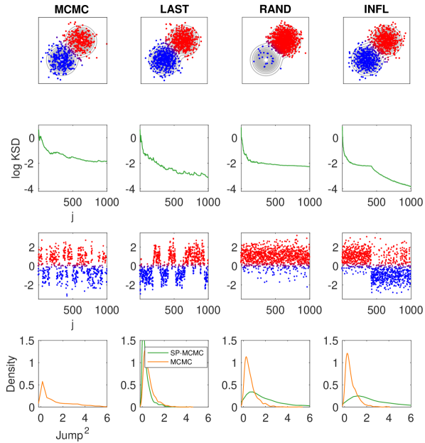
Figure 2: Gaussian mixture experiment in dimension $d=2$. Columns (left to right): MCMC, SP-MCMC with LAST!, SP-MCMC with RAND!, SP-MCMC with INFL!. Top row: Point sets of size $n=1000$ produced by MCMC and SP-MCMC. (Point colour indicates the mode to which they are closest.) Second row: Trace plot of $\log D_{\mathcal{K}_{0},P}(\{x_{i}\}_{i=1}^{j})$ as $j$ is varied from $1$ to $n$. Third row: Trace plots of the sequence $(x_{i})_{i=1}^{n}$, projected onto the first coordinate. Bottom row: Distribution of the squared jump distance $\|x_{j}-x_{j-1}\|_{2}^{2}$ (green) compared to the quantities $\|y_{j,m_{j}}-y_{j,1}\|_{2}^{2}$ associated with the Markov chains (orange) used during the course of each method.

For exposition we let $\sigma^{2}=0.5$ and consider a $d=2$ dimensional Gaussian mixture model $P=\frac{1}{2}\mathcal{N}(-\mathrm{1},\sigma^{2}\mathrm{I}_{d\times d})+\frac{1}{2}\mathcal{N}(\mathrm{1},\sigma^{2}\mathrm{I}_{d\times d})$ with modes at $\mathrm{1}=[1,1]$ and $-\mathrm{1}$. The performance of MCMC was compared to SP-MCMC for each of the criteria LAST, RAND, INFL. Note that in this section we do not address computational cost; this is examined in Secs. 4.3 and 4.4. For SP-MCMC the sequence $(m_{j})_{j\in\mathbb{N}}$ was set as $m_{j}=5$. Results are presented in Fig. 2 with $n=1000$.

The point sets produced by SP-MCMC with LAST and INFL (top row) were observed to provide a better quantisation of the target $P$ compared to MCMC, as captured by the KSD of the empirical measure to the target (second row). RAND did not distribute points evenly between modes and, as a result, KSD was observed to plateau in the range of $n$ displayed. For MCMC, the proposal step-size $h>0$ was optimised according to the recommendations in (Roberts & Rosenthal, 2001), but nevertheless the chain was observed to jump between the two components of $P$ only infrequently (third row, colour-coded). In contrast, after an initial period where both modes are populated, SP-MCMC under the INFL criteria was seen to frequently jump between components of $P$. Finally, we note that under INFL the typical squared jump distance $\|x_{j}-x_{j-1}\|_{2}^{2}$ was greater than the analogous quantities $\|y_{j,m_{j}}-y_{j,1}\|_{2}^{2}$ for the underlying Markov chains that were used (bottom row), despite the latter being optimised according to the recommendations of (Roberts & Rosenthal, 2001), which supports the view that more frequent mode-hopping is a property of the INFL method. Based on the findings of this experiment, we focus only on LAST and INFL in the sequel. The extension where “bad” points are removed, described in Remark 3, was explored in supplemental Section A.6.5.

4.3 IGARCH Model

Next our attention turns to whether SP-MCMC improves over the original SP method and how it compares to existing methods such as MED and SVGD when computational cost is taken into account. To this end we consider an identical experiment to (Chen et al., 2018b), based on Bayesian inference for a classical integrated generalised autoregressive conditional heteroskedasticity (IGARCH) model. The IGARCH model (Taylor, 2011)

$$y_{t} = \sigma_{t}\epsilon_{t},\hskip 40.0pt\epsilon_{t}\stackrel{{\scriptstyle\text{i.i.d.}}}{{\sim}}\mathcal{N}(0,1)$$

$$\sigma_{t}^{2} = \theta_{1}+\theta_{2}y_{t-1}^{2}+(1-\theta_{2})\sigma_{t-1}^{2}$$

describes a financial time series $(y_{t})$ with time-varying volatility $(\sigma_{t})$. The model is parametrised by $\theta=(\theta_{1},\theta_{2})$, $\theta_{1}>0$ and $0<\theta_{2}<1$ and Bayesian inference for $\theta$ is considered, based on data $y=(y_{t})$ that represent 2,000 daily percentage returns of the S&P 500 stock index (from December 6, 2005 to November 14, 2013). Following (Chen et al., 2018b), an improper uniform prior was placed on $\theta$. The domain $\mathcal{X}=\mathbb{R}_{+}\times(0,1)$ is bounded and, for this example, the posterior $P$ places negligible mass near the boundary $\partial\mathcal{X}$. This ensures that the boundary conditions described in Sec. 2.1 hold essentially to machine precision, as argued in (Chen et al., 2018b).

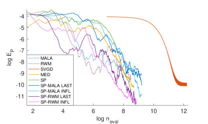
Figure 3: IGARCH experiment. The new SP-MCMC method was compared against the original SP method of (Chen et al., 2018b), as well as against MCMC, MED (Roshan Joseph et al., 2015) and SVGD (Liu & Wang, 2016). The implementation of all existing methods is described in Appendix A.6. Each method produced an empirical measure $\frac{1}{n}\sum_{i=1}^{n}\delta_{x_{i}}$ whose distance to the target $P$ was quantified by the energy distance $E_{P}$. The computational cost was quantified by the number $n_{\text{eval}}$ of times either $\tilde{p}$ or its gradient were evaluated.

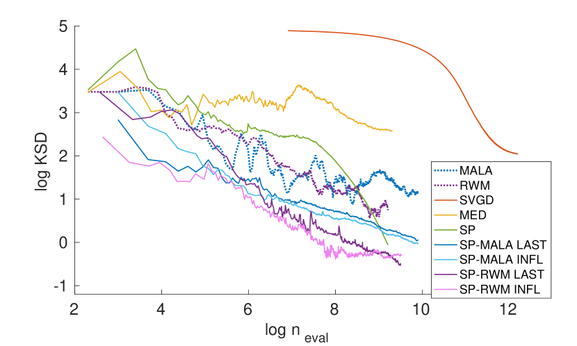
(a) $d=4$

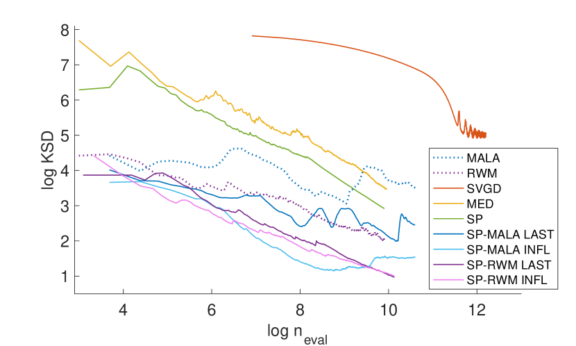
(b) $d=10$

Figure 4: ODE experiment, $d$-dimensional. The new SP-MCMC method was compared against the original SP method of (Chen et al., 2018b), as well as against standard MCMC, MED (Roshan Joseph et al., 2015) and SVGD (Liu & Wang, 2016). Each method produced an empirical measure $\frac{1}{n}\sum_{i=1}^{n}\delta_{x_{i}}$ whose distance to the target $P$ was quantified by the kernel Stein discrepancy (KSD). The computational cost was quantified by the number $n_{\text{eval}}$ of times either $\tilde{p}$ or its gradient were evaluated.

For objectivity, the energy distance $E_{P}$ (Székely & Rizzo, 2004; Baringhaus & Franz, 2004) was used to assess closeness of all empirical measures to the target. SP-MCMC was implemented with $m_{j}=5\;\forall j$. In addition to SP-MCMC, the methods SP, MED, SVGD and standard MCMC were also considered, with implementation described in Appendix A.6. All methods produced a point set of size $n=1000$. The results, presented in Fig. 3, are indexed by the computational cost of running each method, which is a count of the total number $n_{\text{eval}}$ of times either $\tilde{p}$ or $\nabla\log\tilde{p}$ were evaluated. It can be seen that SP-MCMC offers improved performance over the original SP method for fixed computational cost, and in turn over both MED and SVGD in this experiment. Typical point sets produced by each method are displayed in Fig. S1. The performance of the pre-conditioned kernel on this task was investigated in Appendix A.6.4.

4.4 System of Coupled ODEs

Our final example is more challenging and offers an opportunity to explore the limitations of SP-MCMC in higher dimensions. The context is an indirectly observed ODE

$$y_{i} = g(u(t_{i}))+\epsilon_{i},\hskip 18.0pt\epsilon_{i}\stackrel{{\scriptstyle\text{i.i.d.}}}{{\sim}}\mathcal{N}(0,\sigma^{2}\mathrm{I})$$

$$\dot{u}(t) = f_{\theta}(t,u),\hskip 40.0ptu(0)=u_{0}$$

and, in particular, Bayesian inference for the parameter $\theta$ in the gradient field. Here $y_{i}\in\mathbb{R}^{p}$, $u(t)\in\mathbb{R}^{q}$ and $\theta\in\mathbb{R}^{d}$ for $p,q,d\in\mathbb{N}$. For our experiment, $f_{\theta}$ and $g$ comprised two instantiations of the Goodwin oscillator (Goodwin, 1965), one low-dimensional with $(q,d)=(2,4)$ and one higher-dimensional with $(q,d)=(8,10)$. In both cases $p=2$, $\sigma=0.1$ and 40 measurements were observed at uniformly-spaced time points in $[41,80]$. The Goodwin oscillator does not permit a closed form solution, meaning that each evaluation of the likelihood function requires the numerical integration of the ODE at a non-negligible computational cost. SP-MCMC was implemented with the INFL criterion and $m_{j}=10$ ($d=4$), $m_{j}=20$ ($d=10$). Full details of the ODE and settings for MED and SVGD are provided in Appendix A.6.6.

In this experiment, KSD was used to assess closeness of all empirical measures to the target. Naturally, SP and SP-MCMC are favoured by this choice of assessment criterion, as these methods are designed to directly minimise KSD. Therefore our main focus here is on the comparison between SP and SP-MCMC. All methods produced a point set of size $n=1000$. Results are shown in Fig. 4(a) (low-dimensional) and Fig. 4(b) (high-dimensional). Note how the gain in performance of SP-MCMC over SP is more substantial when $d=10$ compared to when $d=4$, supporting our earlier intuition for the advantage of local optimisation using a Markov kernel.

5 Theoretical Results

Let $\Omega$ be a probability space on which the collection of random variables $Y_{j,l}:\Omega\rightarrow\mathcal{X}$ representing the $l^{\text{th}}$ state of the Markov chain run at the $j^{\text{th}}$ iteration of SP-MCMC are defined. Each of the three algorithms that we consider correspond to a different initialisation of these Markov chains and we use $\mathbb{E}$ to denote expectation over randomness in the $Y_{j,l}$. For example, the algorithm called LAST would set $Y_{j,1}(\omega)=x_{j-1}$. It is emphasised that the results of this section hold for any choice of function crit that takes values in $\mathcal{X}$. As a stepping-stone toward our main result, we first extend the theoretical analysis of the original SP method to the case where the global search is replaced by a Monte Carlo search based on $m_{i}$ independent draws from $P$ at iteration $i$ of the SP method.

Theorem 1 (i.i.d. SP-MCMC Convergence).

Suppose that the kernel $k_{0}$ satisfies $\int_{\mathcal{X}}k_{0}(x,\cdot)\mathrm{d}P(x)\equiv 0$ and $\mathbb{E}_{Z\sim P}[e^{\gamma k_{0}(Z,Z)}]<\infty$ for some $\gamma>0$. Let $(m_{j})_{j=1}^{n}\subset\mathbb{N}$ be a fixed sequence, and consider idealised Markov chains with $Y_{j,l}\stackrel{{\scriptstyle\text{\emph{i.i.d.}}}}{{\sim}}P$ for all $1\leq l\leq m_{j}$, $j\in\mathbb{N}$. Let $\{x_{i}\}_{i=1}^{n}$ denote the output of SP-MCMC. Then, writing $a\wedge b=\min\{a,b\}$, $\exists\;C>0$ such that

$$\mathbb{E}\left[D_{\mathcal{K}_{0},P}(\{x_{i}\}_{i=1}^{n})^{2}\right]\leq\textstyle\frac{C}{n}\sum_{i=1}^{n}\frac{\log(n\wedge m_{i})\wedge\sup_{x\in\mathcal{X}}k_{0}(x,x)}{n\wedge m_{i}}.$$

The constant $C$ depends on $k_{0}$ and $P$, and the proof in Appendix A.1 makes this dependence explicit.

It follows that SP-MCMC with independent sampling from $P$ is consistent whenever each $m_{j}$ grows with $n$. When $m_{j}=m$ for all $j$ we obtain:

$$\mathbb{E}\left[D_{\mathcal{K}_{0},P}(\{x_{i}\}_{i=1}^{n})^{2}\right]\leq\textstyle C\frac{\log(n\wedge m)\wedge\sup_{x\in\mathcal{X}}k_{0}(x,x)}{n\wedge m},$$

and by choosing $m=n$, we recover the rate (5) of the original SP algorithm which optimizes over all of $\mathcal{X}$ (Chen et al., 2018b). For bounded kernels, the result improves over the $O(1/n+1/\sqrt{m})$ independent sampling kernel herding rate established in (Lacoste-Julien et al., 2015, App. B). Thm. 1 more generally accommodates unbounded kernels at the cost of a $\log(n\wedge m)$ factor.

The role of Thm. 1 is limited to providing a stepping stone to Thm. 2, as it is not practical to obtain exact samples from $P$ in general. To state our result in the general case, restrict attention to $\mathcal{X}=\mathbb{R}^{d}$, consider a function $V:\mathcal{X}\to[1,\infty)$ and define the associated operators $\|f\|_{V}:=\sup_{x\in\mathcal{X}}|f(x)|/V(x)$, $\|\mu\|_{V}:=\sup_{f:\|f\|_{V}\leq 1}|\int f\mathrm{d}\mu|$ respectively on functions $f:\mathcal{X}\rightarrow\mathbb{R}$ and on signed measures $\mu$ on $\mathcal{X}$. A Markov chain $(Y_{i})_{i\in\mathbb{N}}\subset\mathcal{X}$ with $n$th step transition kernel $\mathrm{P}^{n}$ is called $V$-uniformly ergodic (Meyn & Tweedie, 2012, Chap. 16) if $\exists R\in[0,\infty),\rho\in(0,1)$ such that $\|\mathrm{P}^{n}(y,\cdot)-P\|_{V}\leq RV(y)\rho^{n}$ for all initial states $y\in\mathcal{X}$ and all $n\in\mathbb{N}$. The proof of the following is provided in Appendix A.2:

Theorem 2 (SP-MCMC Convergence).

Suppose $\int_{\mathcal{X}}k_{0}(x,\cdot)\mathrm{d}P(x)\equiv 0$ with $\mathbb{E}_{Z\sim P}[e^{\gamma k_{0}(Z,Z)}]<\infty$ for $\gamma>0$. For a sequence $(m_{j})_{j=1}^{n}\subset\mathbb{N}$, let $\{x_{i}\}_{i=1}^{n}$ denote the output of SP-MCMC, based on time-homogeneous reversible Markov chains $(Y_{j,l})_{l=1}^{m_{j}}$, $j\in\mathbb{N}$, generated using the same $V$-uniformly ergodic transition kernel. Define $V_{\pm}(s):=\sup_{x:k_{0}(x,x)\leq s^{2}}k_{0}(x,x)^{1/2}V(x)^{\pm 1}$ and $S_{i}=\sqrt{2\log(n\wedge m_{i})/\gamma}$. Then $\exists\;C>0$ such that

$$\mathbb{E}\left[D_{\mathcal{K}_{0},P}(\{x_{i}\}_{i=1}^{n})^{2}\right]\leq\textstyle\frac{C}{n}\sum_{i=1}^{n}\frac{S_{i}^{2}}{n}+\frac{V_{+}(S_{i})V_{-}(S_{i})}{m_{i}}.$$

We give an example of verifying the preconditions of Thm. 2 for MALA. Let $\mathcal{P}$ denote the set of distantly dissipative distributions with $\nabla\log p$ Lipschitz on $\mathcal{X}=\mathbb{R}^{d}$. Let $C_{b}^{(r,r)}$ be the set of functions $k:\mathbb{R}^{d}\times\mathbb{R}^{d}\rightarrow\mathbb{R}$ with $(x,y)\mapsto\nabla_{x}^{l}\nabla_{y}^{l}k(x,y)$ continuous and uniformly bounded for $l\in\{0,\dots,r\}$. Let $q(x,y)$ be a density for the proposal distribution of MALA, and let $\alpha(x,y)$ denote the acceptance probability for moving from $x$ to $y$, given that $y$ has been proposed. Let $A(x)=\{y\in\mathcal{X}:\alpha(x,y)=1\}$ denote the region where proposals are always accepted and let $R(x)=\mathcal{X}\setminus A(x)$. Let $I(x):=\{y:\|y\|_{2}\leq\|x\|_{2}\}$. MALA is said to be inwardly convergent (Roberts & Tweedie, 1996, Sec. 4) if

$$\lim_{\|x\|_{2}\rightarrow\infty}\int_{A(x)\Delta I(x)}q(x,y)\mathrm{d}y=0$$ (7)

where $A\Delta B$ denotes the symmetric set difference $(A\cup B)\setminus(A\cap B)$. The proof of the following is provided in Appendix A.3:

Theorem 3 (SP-MALA Convergence).

Suppose $k_{0}$ has the form 3, based on a kernel $k\in C_{b}^{(1,1)}$ and a target $P\in\mathcal{P}$ such that $\int_{\mathcal{X}}k_{0}(x,\cdot)\mathrm{d}P(x)\equiv 0$. Let $(m_{j})_{j=1}^{n}\subset\mathbb{N}$ be a fixed sequence and let $\{x_{i}\}_{i=1}^{n}$ denote the output of SP-MCMC, based on Markov chains $(Y_{j,l})_{l=1}^{m_{j}}$, $j\in\mathbb{N}$, generated using MALA transition kernel with step size $h$ sufficiently small. Assume $P$ is such that MALA is inwardly convergent. Then MALA is $V$-uniformly ergodic for $V(x)=1+\|x\|_{2}$ and $\exists\;C>0$ such that

$$\mathbb{E}\left[D_{\mathcal{K}_{0},P}(\{x_{i}\}_{i=1}^{n})^{2}\right]\leq\textstyle\frac{C}{n}\sum_{i=1}^{n}\frac{\log(n\wedge m_{i})}{n\wedge m_{i}}.$$

Our final result, proved in Appendix A.4, establishes that the pre-conditioner kernel proposed in Sec. 3.2 can control weak congergence to $P$ when the pre-conditionner $\Lambda$ is symmetric positive definite (denoted $\Lambda\succ 0$). It is a generalisation of Thm. 8 of Gorham & Mackey (2017), who treated the special case of $\Lambda=I$:

Theorem 4 (Pre-conditioned IMQ KSD Controls Convergence).

Suppose $k_{0}$ is a Stein kernel 3 for a target $P\in\mathcal{P}$ and a pre-conditioned IMQ base kernel 6 with $\beta\in(-1,0)$ and $\Lambda\succ 0$. If $D_{\mathcal{K}_{0},P}(\{x_{i}\}_{i=1}^{n})\rightarrow 0$ then $\frac{1}{n}\sum_{i=1}^{n}\delta_{x_{i}}$ converges weakly to $P$.

6 Conclusion

This paper proposed fundamental improvements to the SP method of (Chen et al., 2018b), establishing, in particular, that the global search used to select each point can be replaced with a finite-length sample path from an MCMC method. The convergence of the proposed SP-MCMC method was established, with an explicit bound provided on the KSD in terms of the $V$-uniform ergodicity of the Markov transition kernel.

Potential extensions to our SP-MCMC method include the use of fast approximate Markov kernels for $P$ (such as the unadjusted Langevin algorithm; see Appendix A.3), fast approximations to KSD (Jitkrittum et al., 2017; Huggins & Mackey, 2018), exploitation of conditional independence structure in $P$ (Wang et al., 2018; Zhuo et al., 2018) and extension to a general Riemannian manifold $\mathcal{X}$ (Liu & Zhu, 2018; Barp et al., 2018b). One could also attempt to use our MCMC optimization approach to accelerate related algorithms such as kernel herding (Chen et al., 2010; Bach et al., 2012; Lacoste-Julien et al., 2015). Other recent approaches to quantisation in the Bayesian context include (Futami et al., 2018; Hu et al., 2018; Frogner & Poggio, 2018; Zhang et al., 2018; Chen et al., 2018a; Li et al., 2019), and an assessment of the relative performance of these methods would be of interest. However, we note that these approaches are not accompanied by the same level of theoretical guarantees that we have established.

Appendix A Supplementary Material

In this supplement, Sections A.1, A.2, A.3 and A.4 contain complete proofs for the results stated in the main text, Section A.5 details the Markov transition kernel that was used in all experiments and Section A.6 contains an in-depth presentation of our empirical results which were summarised at a high level in the main text.

A.1 Proof of Theorem 1

Note that the performance of greedy algorithms for minimisation of MMD was studied in (De Marchi et al., 2005; Santin & Haasdonk, 2017). Our analysis, and that in (Chen et al., 2018b), differ in several respects from this work - not least in that our arguments do not require the set $\mathcal{X}$ to be compact.

First, we state and prove a generalisation of Theorem 5 in (Chen et al., 2018b), which quantifies KSD convergence for point sets produced by approximately optimizing over arbitrary subsets of $\mathcal{X}$:

Theorem 5 (Generalized Stein Point Convergence).

Suppose $k_{0}$ is a reproducing kernel with $\int_{\mathcal{X}}k_{0}(x,\cdot)\mathrm{d}P(x)\equiv 0$. Fix $n\in\mathbb{N}$, and, for each $1\leq j\leq n$, any $\mathcal{Y}_{j}\subseteq\mathcal{X}$ and any $h_{j}$ in the convex hull of $\{k_{0}(x,\cdot)\}_{x\in\mathcal{Y}_{j}}$. Fix $\delta>0$ and, for each $1\leq i\leq n$, fix $S_{i}\geq 0$ and $r_{i}>0$. Any point set $\{x_{i}\}_{i=1}^{n}\subset\mathcal{X}$ satisfying

$$\frac{k_{0}(x_{j},x_{j})}{2} +\displaystyle\sum_{i=1}^{j-1}k_{0}(x_{i},x_{j})\leq\frac{\delta}{2}+\frac{S_{j}^{2}}{2}+\displaystyle\inf_{x\in\mathcal{Y}_{j}}\displaystyle\sum_{i=1}^{j-1}k_{0}(x_{i},x)$$ (8)

for each $1\leq j\leq n$ also satisfies

$$D_{\mathcal{K}_{0},P}(\{x_{i}\}_{i=1}^{n})\leq\exp\left(\frac{1}{2}\sum_{j=1}^{n}\frac{1}{r_{j}}\right)\sqrt{\frac{\delta}{n}+\frac{1}{n^{2}}\sum_{i=1}^{n}\left(S_{i}^{2}+r_{i}\|h_{i}\|_{\mathcal{K}_{0}}^{2}\right)}.$$ (9)

Proof.

Let $a_{n}:=n^{2}D_{\mathcal{K}_{0},P}(\{x_{i}\}_{i=1}^{n})^{2}=\sum_{i=1}^{n}\sum_{i^{\prime}=1}^{n}k_{0}(x_{i},x_{i^{\prime}})=\|\sum_{i=1}^{n}k_{0}(x_{i},\cdot)\|^{2}_{\mathcal{K}_{0}}$. Then

$$a_{n}\;=\;\sum_{i=1}^{n}\sum_{i^{\prime}=1}^{n}k_{0}(x_{i},x_{i^{\prime}})\;=\;a_{n-1}+k_{0}(x_{n},x_{n})+2\sum_{i=1}^{n-1}k_{0}(x_{i},x_{n})\;\leq\;a_{n-1}+\delta+S_{n}^{2}+2\inf_{x\in\mathcal{Y}_{n}}\sum_{i=1}^{n-1}k_{0}(x_{i},x),$$ (10)

where for the final inequality we have used (8) with $j=n$. Next, we let $f_{n}:=\sum_{i=1}^{n}k_{0}(x_{i},\cdot)$ so that $\|f_{n}\|_{\mathcal{K}_{0}}=\sqrt{a_{n}}$. Applying in the first instance the Cauchy-Schwarz inequality, then making use of the arithmetic-geometric inequality, we get:

$$2\inf_{x\in\mathcal{Y}_{n}}f_{n-1}(x)\;=\;2\inf_{f\in\mathcal{M}_{n}}\langle f_{n-1},f\rangle_{\mathcal{K}_{0}}\; \leq\;2\langle f_{n-1},h_{n}\rangle_{\mathcal{K}_{0}}$$

$$\leq 2\;\sqrt{\|f_{n-1}\|^{2}_{\mathcal{K}_{0}}\|h_{n}\|^{2}_{\mathcal{K}_{0}}}\;=2\;\sqrt{\left(\frac{\|f_{n-1}\|^{2}_{\mathcal{K}_{0}}}{r_{n}}\right)(r_{n}\|h_{n}\|^{2}_{\mathcal{K}_{0}})}$$

$$\leq\;r_{n}\|h_{n}\|_{\mathcal{K}_{0}}^{2}+\frac{a_{n-1}}{r_{n}}.$$ (11)

Combining (10) and (11) establishes the recurrence relation

$$a_{n}\leq\left(1+\frac{1}{r_{n}}\right)a_{n-1}+\delta+S_{n}^{2}+r_{n}\|h_{n}\|_{\mathcal{K}_{0}}^{2}.$$ (12)

Expanding the recurrence leads to a product of terms of the form $(1+\frac{1}{r_{n}})$ which must be controlled. To this end, we use the fact that $\log(1+x)\leq x$ for $x\geq 0$ implies that

$$\log\prod_{j=1}^{n}\left(1+\frac{1}{r_{j}}\right)\;=\;\sum_{j=1}^{n}\log\left(1+\frac{1}{r_{j}}\right)\;\leq\;\sum_{j=1}^{n}\frac{1}{r_{j}},$$

and, noting that the function $i\mapsto\prod_{j=1}^{i}(1+1/r_{n-j+1})$ is increasing, we can bound the product

$$\prod_{j=1}^{i}\left(1+\frac{1}{r_{n-j+1}}\right)\;\leq\;\prod_{j=1}^{n}\left(1+\frac{1}{r_{j}}\right)\;\leq\;\exp\left(\sum_{j=1}^{n}\frac{1}{r_{j}}\right),$$

uniformly in $i$. This implies that the recurrence relation in (12) satisfies

$$a_{n} \leq \sum_{i=0}^{n-1}\left(\delta+S_{n-i}^{2}+r_{n-i}\|h_{n-i}\|_{\mathcal{K}_{0}}^{2}\right)\prod_{j=1}^{i}\left(1+\frac{1}{r_{n-j+1}}\right)$$

$$\leq \exp\left(\sum_{j=1}^{n}\frac{1}{r_{j}}\right)\sum_{i=0}^{n-1}\left(\delta+S_{n-i}^{2}+r_{n-i}\|h_{n-i}\|_{\mathcal{K}_{0}}^{2}\right),$$

from which the result is established. ∎

Theorem 5 is a refinement of the argument used in the first part of the proof of Theorem 5 in (Chen et al., 2018b). It serves to make explicit the roles of $S_{j}$ and $\|h_{j}\|_{\mathcal{K}_{0}}$ and distinguishes between the content of (9) and subsequent assumptions on $k_{0}$ and $P$ that are used to bound the terms that are involved.

The result of Theorem 5 provides an upper bound in the situation where the sets $\mathcal{Y}_{j}$ are fixed. To make use of Theorem 5 in the context of SP-MCMC, where the sets $\mathcal{Y}_{j}$ are instead randomly generated, we must therefore establish probabilistic bounds on the quantities $S_{i}$ and $\|h_{i}\|_{\mathcal{K}_{0}}$ that appear in the statement of Theorem 5. This is the content of the next result:

Theorem 6 (Generalized i.i.d. SP-MCMC Convergence).

Suppose $k_{0}$ is a reproducing kernel with $\int_{\mathcal{X}}k_{0}(x,\cdot)\mathrm{d}P(x)\equiv 0$ and $\mathbb{E}_{Z\sim P}[e^{\gamma k_{0}(Z,Z)}]<\infty$. Fix a sequence $(m_{j})_{j=1}^{n}\subset\mathbb{N}$ and, for each $j\in\mathbb{N}$, let $\mathcal{Y}_{j}$ be the set of independent random variables $\{Y_{j,l}\}_{l=1}^{m_{j}}$, with each $Y_{j,l}\sim P$. For each $1\leq i\leq n$, fix $\tilde{S}_{i}\geq 0$ and $r_{i}>0$. Then $\exists C>0$ such that

$$\mathbb{E}\left[D_{\mathcal{K}_{0},P}(\{x_{i}\}_{i=1}^{n})^{2}\right]\;\leq\;C\exp\Bigg{(}\sum_{j=1}^{n}\frac{1}{r_{j}}\Bigg{)}\frac{1}{n^{2}}\sum_{i=1}^{n}\left(r_{i}e^{-\frac{\gamma}{2}\tilde{S}_{i}^{2}}+\left(1+\frac{r_{i}}{m_{i}}\right)\min\left\{\tilde{S}_{i}^{2},\sup_{x\in\mathcal{X}}k_{0}(x,x)\right\}\right),$$ (13)

where in each case the total expectation $\mathbb{E}$ is taken over realisations of the random sets $\mathcal{Y}_{j}$, $j\in\mathbb{N}$.

Proof.

Recall that the $j$th iteration of SP-MCMC requires that random variables $(Y_{j,l})_{l=1}^{m_{j}}$ are instantiated. Define the set $\mathcal{Y}_{j}$ to consist of the subset of these $m_{j}$ samples for which $Y_{j,l}\in B_{j}:=\{x\in\mathcal{X}:k_{0}(x,x)\leq\tilde{S}_{j}^{2}\}$ is satisfied. Note that SP-MCMC selects the $j$th point $x_{j}$ from the collection $\{Y_{j,l}\}_{l=1}^{m_{j}}$ such that

$$\frac{k_{0}(x_{j},x_{j})}{2}+\displaystyle\sum_{i=1}^{j-1}k_{0}(x_{i},x_{j}) =\displaystyle\inf_{x\in\{Y_{j,l}:l=1,\dots,m_{j}\}}\frac{k_{0}(x,x)}{2}+\displaystyle\sum_{i=1}^{j-1}k_{0}(x_{i},x)$$

$$\leq\displaystyle\inf_{x\in\mathcal{Y}_{j}}\frac{k_{0}(x,x)}{2}+\displaystyle\sum_{i=1}^{j-1}k_{0}(x_{i},x)\;\leq\;\frac{1}{2}\min\left\{\tilde{S}_{j}^{2},\sup_{x\in\mathcal{X}}k_{0}(x,x)\right\}+\displaystyle\inf_{x\in\mathcal{Y}_{j}}\displaystyle\sum_{i=1}^{j-1}k_{0}(x_{i},x).$$

so that (8) is satisfied with $\delta=0$ and $S_{j}:=\min\left\{\tilde{S}_{j},\sup_{x\in\mathcal{X}}k_{0}(x,x)^{1/2}\right\}$.

Let $h_{j}(\cdot):=\frac{1}{m_{j}}\sum_{l=1}^{m_{j}}k_{0}(Y_{j,l},\cdot)\mathbb{I}[Y_{j,l}\in B_{j}]$, which is an element of the convex hull of $\{k_{0}(x,\cdot)\}_{x\in\mathcal{Y}_{j}}$. Define also the truncated kernel mean embeddings

$$k_{j}^{-}(\cdot):=\int k_{0}(x,\cdot)\mathbb{I}[x\in B_{j}]\mathrm{d}P(x),\qquad k_{j}^{+}(\cdot):=\int k_{0}(x,\cdot)\mathbb{I}[x\notin B_{j}]\mathrm{d}P(x).$$

From the triangle inequality followed by Jensen’s inequality

$$\|h_{j}\|_{\mathcal{K}_{0}}^{2} \leq 2\left(\|k_{j}^{-}\|_{\mathcal{K}_{0}}^{2}+\|h_{j}-k_{j}^{-}\|_{\mathcal{K}_{0}}^{2}\right).$$ (14)

In what follows we aim to bound the two terms on the right hand side of (14).

Bound on $\|k_{j}^{-}\|_{\mathcal{K}_{0}}^{2}$:

For the first term in (14), since $\int_{\mathcal{X}}k_{0}(x,\cdot)\mathrm{d}P(x)\equiv 0$ we have $k_{j}^{+}=-k_{j}^{-}$. Thus, we deduce that

$$\|k_{j}^{-}\|_{\mathcal{K}_{0}}^{2}=\|k_{j}^{+}\|_{\mathcal{K}_{0}}^{2} =\iint k_{0}(x,y)\mathbb{I}[x\notin B_{j}]\mathrm{d}P(x)\mathbb{I}[y\notin B_{j}]\mathrm{d}P(y)$$

$$\leq\left(\int\sqrt{k_{0}(x,x)}\mathbb{I}[x\notin B_{j}]\mathrm{d}P(x)\right)^{2}\;\leq\;\int k_{0}(x,x)\mathbb{I}[x\notin B_{j}]\mathrm{d}P(x)$$

where the final two inequalities follow by Cauchy-Schwarz and Jensen’s inequality. Now, let $Y=k_{0}(Z,Z)$ for $Z\sim P$ and $b:=\mathbb{E}[e^{\gamma Y}]<\infty$. Following Appendix A.1.3 of (Chen et al., 2018b), we will bound the tail expectation above by considering the biased random variable $Y^{*}=k_{0}(Z^{*},Z^{*})$ for $Z^{*}$ with density

$$\rho(z^{*})=\frac{k_{0}(z^{*},z^{*})p(z^{*})}{\mathbb{E}[Y]}.$$

To this end we have, by the relation $x\leq e^{x}$,

$$\mathbb{E}[e^{\frac{\gamma}{2}Y^{*}}]=\mathbb{E}[e^{\frac{\gamma}{2}k_{0}(Z^{*},Z^{*})}]=\frac{\mathbb{E}[k_{0}(Z,Z)e^{\frac{\gamma}{2}k_{0}(Z,Z)}]}{\mathbb{E}[Y]}=\frac{\mathbb{E}[\frac{\gamma}{2}Ye^{\frac{\gamma}{2}Y}]}{\frac{\gamma}{2}\mathbb{E}[Y]}\leq\frac{\mathbb{E}[e^{\gamma Y}]}{\lambda\mathbb{E}[Y]}=\frac{2b}{\gamma\mathbb{E}[Y]}.$$

From an application of Markov’s inequality we see that

$$\mathbb{P}[Y^{*}\geq\tilde{S}_{j}^{2}]=\mathbb{P}[e^{\frac{\gamma}{2}Y^{*}}\geq e^{\frac{\gamma}{2}\tilde{S}_{j}^{2}}]\leq\frac{\mathbb{E}[e^{\frac{\gamma}{2}Y^{*}}]}{e^{\frac{\gamma}{2}\tilde{S}_{j}^{2}}}\leq\frac{2b}{\gamma\mathbb{E}[Y]}e^{-\frac{\gamma}{2}\tilde{S}_{j}^{2}}$$

and as a consequence

$$\|k_{j}^{-}\|_{\mathcal{K}_{0}}^{2}\leq\int k_{0}(x,x)\mathbb{I}[k_{0}(x,x)>\tilde{S}_{j}^{2}]\mathrm{d}P(x)={\mathbb{E}[Y]}\int\mathbb{I}[k_{0}(x,x)>\tilde{S}_{j}^{2}]\rho(x)\mathrm{d}x={\mathbb{E}[Y]}\mathbb{P}[Y^{*}\geq\tilde{S}_{j}^{2}]\leq\frac{2b}{\gamma}e^{-\frac{\gamma}{2}\tilde{S}_{j}^{2}}.$$ (15)

Bound on $\|h_{j}-k_{j}^{-}\|_{\mathcal{K}_{0}}^{2}$:

For the second term in (14), we have that

$$\|h_{j}-k_{j}^{-}\|_{\mathcal{K}_{0}}^{2} = \frac{1}{m_{j}^{2}}\sum_{l,l^{\prime}=1}^{m_{j}}k_{0}(Y_{j,l},Y_{j,l^{\prime}})\mathbb{I}[Y_{j,l},Y_{j,l^{\prime}}\in B_{j}]-\frac{2}{m_{j}}\sum_{l=1}^{m_{j}}\int k_{0}(x,Y_{j,l})\mathbb{I}[x,Y_{j,l}\in B_{j}]\mathrm{d}P(x)$$

$$+\iint k_{0}(x,x^{\prime})\mathbb{I}[x,x^{\prime}\in B_{j}]\mathrm{d}P(x)\mathrm{d}P(x^{\prime})$$

$$= \frac{1}{m_{j}}\sum_{l=1}^{m_{j}}\left\{\frac{1}{m_{j}}\sum_{l^{\prime}=1}^{m_{j}}k_{0}(Y_{j,l},Y_{j,l^{\prime}})\mathbb{I}[Y_{j,l},Y_{j,l^{\prime}}\in B_{j}]-\int k_{0}(x,Y_{j,l})\mathbb{I}[x,Y_{j,l}\in B_{j}]\mathrm{d}P(x)\right\}$$

$$-\int\left\{\frac{1}{m_{j}}\sum_{l=1}^{m_{j}}k_{0}(x,Y_{j,l})\mathbb{I}[x,Y_{j,l}\in B_{j}]-\int k_{0}(x,x^{\prime})\mathbb{I}[x,x^{\prime}\in B_{j}]\mathrm{d}P(x^{\prime})\right\}\mathrm{d}P(x)$$

$$= \frac{1}{m_{j}^{2}}\sum_{l=1}^{m_{j}}\sum_{l^{\prime}=1}^{m_{j}}\left\{h_{Y_{j,l^{\prime}}}(Y_{j,l})-\int h_{Y_{j,l}}(x)\mathrm{d}P(x)\right\}-\frac{1}{m_{j}}\sum_{l=1}^{m_{j}}\int\left\{h_{x}(Y_{j,l})-\int h_{x}(x^{\prime})\mathrm{d}P(x^{\prime})\right\}\mathrm{d}P(x)$$

$$= \frac{1}{m_{j}^{2}}\sum_{l=1}^{m_{j}}\sum_{l^{\prime}=1}^{m_{j}}\left\{h_{Y_{j,l^{\prime}}}(Y_{j,l})-\int h_{Y_{j,l^{\prime}}}(x)\mathrm{d}P(x)\right\}-\frac{1}{m_{j}}\sum_{l=1}^{m_{j}}\int\left\{h_{x}(Y_{j,l})-\int h_{x}(x^{\prime})\mathrm{d}P(x^{\prime})\right\}\mathrm{d}P(x)$$

where $h_{x}(x^{\prime}):=k_{0}(x,x^{\prime})\mathbb{I}[x,x^{\prime}\in B_{j}]$. Thus, letting again $Z\sim P$ be independent of all other random variables that we have defined,

$$\mathbb{E}\left[\|h_{j}-k_{j}^{-}\|_{\mathcal{K}_{0}}^{2}\right]=\frac{1}{m_{j}^{2}}\sum_{l=1}^{m_{j}}\sum_{l^{\prime}=1}^{m_{j}}\left\{\mathbb{E}[h_{Y_{j,l^{\prime}}}(Y_{j,l})]-\mathbb{E}[h_{Y_{j,l^{\prime}}}(Z)]\right\}-\frac{1}{m_{j}}\sum_{l=1}^{m_{j}}\int\left\{\mathbb{E}[h_{x}(Y_{j,l})]-\mathbb{E}[h_{x}(Z)]\right\}\mathrm{d}P(x).$$ (16)

Since the $Y_{j,l}$ are assumed to be independent and distributed according to $P$, all of the terms in (16) vanish apart from the diagonal terms in the first sum, and moreover all of the diagonal terms are identical:

$$\mathbb{E}\left[\|h_{j}-k_{j}^{-}\|_{\mathcal{K}_{0}}^{2}\right]=\frac{1}{m_{j}^{2}}\sum_{l=1}^{m_{j}}\left\{\mathbb{E}[h_{Y_{j,l}}(Y_{j,l})]-\mathbb{E}[h_{Y_{j,l}}(Z)]\right\}=\frac{1}{m_{j}}\left\{\mathbb{E}[h_{Y_{j,1}}(Y_{j,1})]-\mathbb{E}[h_{Y_{j,1}}(Z)]\right\}.$$

An application of the triangle inequality and Cauchy-Schwarz leads us to the bound

$$\left|\mathbb{E}\left[\|h_{j}-k_{j}^{-}\|_{\mathcal{K}_{0}}^{2}\right]\right| \leq \frac{1}{m_{j}}\left\{\left|\mathbb{E}[h_{Y_{j,1}}(Y_{j,1})]\right|+\left|\mathbb{E}[h_{Y_{j,1}}(Z)]\right|\right\}$$

$$= \frac{1}{m_{j}}\left\{\left|\mathbb{E}[k_{0}(Y_{j,1},Y_{j,1})\mathbb{I}[Y_{j,1}\in B_{j}]]\right|+\left|\mathbb{E}[k_{0}(Y_{j,1},Z)\mathbb{I}[Y_{j,1},Z\in B_{j}]]\right|\right\}$$

$$\leq \frac{1}{m_{j}}\left\{\mathbb{E}[k_{0}(Y_{j,1},Y_{j,1})\mathbb{I}[Y_{j,1}\in B_{j}]]+\mathbb{E}[k_{0}(Y_{j,1},Y_{j,1})^{\frac{1}{2}}k_{0}(Z,Z)^{\frac{1}{2}}\mathbb{I}[Y_{j,1},Z\in B_{j}]]\right\}$$

$$\leq \frac{2}{m_{j}}\min\left\{\tilde{S}_{j}^{2},\sup_{x\in\mathcal{X}}k_{0}(x,x)\right\}.$$

Overall Bound:

Combining our bounds for the terms in (14) leads to

$$\mathbb{E}[\|h_{j}\|_{\mathcal{K}_{0}}^{2}]\;\leq\;2\left(\|k_{j}^{-}\|_{\mathcal{K}_{0}}^{2}+\mathbb{E}\left[\|h_{j}-k_{j}^{-}\|_{\mathcal{K}_{0}}^{2}\right]\right)\;\leq\;\frac{4b}{\gamma}e^{-\frac{\gamma}{2}\tilde{S}_{j}^{2}}+\frac{4}{m_{j}}\min\left\{\tilde{S}_{j}^{2},\sup_{x\in\mathcal{X}}k_{0}(x,x)\right\}.$$ (17)

Finally, we square the conclusion (9) of Theorem 5 (with, recall, $\delta=0$ and $S_{j}:=\min\{\tilde{S}_{j},\sup_{x\in\mathcal{X}}k_{0}(x,x)^{1/2}\}$) and take expectations, which combine with (17) to produce (13) with $C=\max\left\{\frac{4b}{\gamma},4\right\}$. ∎

Now we are in a position to prove Theorem 1, which follows as a specific instance of Theorem 6:

Proof of Theorem 1.

The result follows as a special case of the general result of Theorem 6 with $S_{i}=\sqrt{\frac{2}{\gamma}\log(n\wedge m_{i})}$ and $r_{i}=n$ for $i=1,\dots,n$. Indeed, with these settings we can bound the conclusion (13) of Theorem 6 as follows (with $C$ a generic constant):

$$\mathbb{E}\left[D_{\mathcal{K}_{0},P}(\{x_{i}\}_{i=1}^{n})^{2}\right] \leq C\exp\Bigg{(}\sum_{j=1}^{n}\frac{1}{r_{j}}\Bigg{)}\frac{1}{n^{2}}\sum_{i=1}^{n}\left(r_{i}e^{-\frac{\gamma}{2}S_{i}^{2}}+\left(1+\frac{r_{i}}{m_{i}}\right)\min\left\{S_{i}^{2},\sup_{x\in\mathcal{X}}k_{0}(x,x)\right\}\right)$$

$$= C\frac{1}{n^{2}}\sum_{i=1}^{n}\left(\frac{n}{n\wedge m_{i}}+\left(1+\frac{n}{m_{i}}\right)\min\left\{\frac{2}{\gamma}\log(n\wedge m_{i}),\sup_{x\in\mathcal{X}}k_{0}(x,x)\right\}\right)$$

$$\leq C\frac{1}{n}\sum_{i=1}^{n}\left(\frac{1}{n\wedge m_{i}}+\frac{1}{n\wedge m_{i}}\min\left\{\log(n\wedge m_{i}),\sup_{x\in\mathcal{X}}k_{0}(x,x)\right\}\right)$$

$$\leq C\frac{1}{n}\sum_{i=1}^{n}\frac{1}{n\wedge m_{i}}\min\left\{\log(n\wedge m_{i}),\sup_{x\in\mathcal{X}}k_{0}(x,x)\right\}$$

as claimed. ∎

To conclude this section, we remark that the general result established in Thm. 6 also implies conditions under which Monte Carlo search strategies can be successfully applied to the Stein Herding algorithm proposed in (Chen et al., 2018b). However, our focus on the greedy version of SP in this work was motivated by the stronger theoretical guarantees posessed by the greedy method, as well as the superior empirical performance reported in (Chen et al., 2018b).

A.2 Proof of Theorem 2

Now we turn to the main task of establishing consistency of SP-MCMC in the Markov chain context. Necessarily, any quantitative result must depend on mixing properties of the Markov chain being used. In this research we focused on time-homogeoeus Markov chains and the notion of mixing called $V$-uniform ergodicity, defined in Sec. 5 of the main text. Recall that, for a function $V:\mathcal{X}\to[1,\infty)$, $V$-uniform ergodicy is the property that

$$\|\mathrm{P}^{n}(y,\cdot)-P\|_{V}\leq RV(y)\rho^{n}$$

for some $R\in[0,\infty)$ and $\rho\in(0,1)$ and for all initial states $y\in\mathcal{X}$ and all $n\in\mathbb{N}$. The assumption of $V$-uniform ergodicity enables us to provide results that hold for any choice of function crit that takes values in $\mathcal{X}$. This includes the functions LAST, RAND and INFL from the main text, but in general the value of crit$(\{x_{i}\}_{i=1}^{j})$ is not restricted to be in $\{x_{i}\}_{i=1}^{j}$ and can be an arbitrary point in $\mathcal{X}$. This permits the development of quite general strategies for SP-MCMC, beyond those explicitly conisdered in the main text.

Armed with the notion of $V$-uniform ergodicity, we derive the following general result:

Theorem 7 (SP-MCMC for $V$-Uniformly Ergodic Markov Chains).

Suppose $\int_{\mathcal{X}}k_{0}(x,\cdot)\mathrm{d}P(x)\equiv 0$ and let $(m_{j})_{j=1}^{n}\subset\mathbb{N}$ be a fixed sequence. Fix a function $V:\mathcal{X}\rightarrow[1,\infty)$ and consider time-homogeneous reversible Markov chains $(Y_{j,l})_{l=1}^{m_{j}}$, $j\in\mathbb{N}$, generated using the same $V$-uniformly ergodic transition kernel. Suppose $\exists\gamma>0$ such that $b:=\mathbb{E}[e^{\gamma k_{0}(Y,Y)}]<\infty$. Let $\{x_{i}\}_{i=1}^{n}$ denote the output of SP-MCMC. For each $1\leq i\leq n$, fix $S_{i}\geq 0$ and $r_{i}>0$. Then for some constant $C$,

$$\mathbb{E}\left[D_{\mathcal{K}_{0},P}(\{x_{i}\}_{i=1}^{n})^{2}\right]\leq C\exp\left(\sum_{i=1}^{n}\frac{1}{r_{i}}\right)\frac{1}{n^{2}}\sum_{i=1}^{n}\left(S_{i}^{2}+r_{i}e^{-\frac{\gamma}{2}S_{i}^{2}}+V_{+}(S_{i})V_{-}(S_{i})\frac{r_{i}}{m_{i}}\right)$$ (18)

where in each case the total expectation $\mathbb{E}$ is taken over realisations of the random sets $\mathcal{Y}_{j}=\{Y_{j,l}\}_{l=1}^{m_{j}}$, $j\in\mathbb{N}$.

Proof.

The stucture of the proof is initially identical to that used in Theorem 6. Indeed, proceeding as in the proof of Theorem 6 we set up the triangle inequality in (14) and attempt to control both terms in this bound. For the first term we proceed identically to obtain the bound on $\|k_{j}^{-}\|_{\mathcal{K}_{0}}^{2}$ in (15). For the second term we proceed identically to obtain the bound

$$\mathbb{E}\left[\|h_{j}-k_{j}^{-}\|_{\mathcal{K}_{0}}^{2}\right]=\frac{1}{m_{j}^{2}}\sum_{l=1}^{m_{j}}\sum_{l^{\prime}=1}^{m_{j}}\left\{\mathbb{E}[h_{Y_{j,l^{\prime}}}(Y_{j,l})]-\mathbb{E}[h_{Y_{j,l^{\prime}}}(Z)]\right\}-\frac{1}{m_{j}}\sum_{l=1}^{m_{j}}\int\left\{\mathbb{E}[h_{x}(Y_{j,l})]-\mathbb{E}[h_{x}(Z)]\right\}\mathrm{d}P(x)$$ (19)

from (16), where $Z\sim P$ is independent of all other random variables that we have defined. However, the subsequent argument in Theorem 6 exploited independence of the random variables $Y_{j,l}$, which does not hold in the Markov chain context. Thus our aim in the sequel is to leverage $V$-uniform ergodicity to control (19).

For the first term in (19) we exploit the definition of the $\|\cdot\|_{V}$ norm and the Cauchy-Schwarz inequality to see that, for each $l^{\prime}\geq l$, we have that

$$\left|\mathbb{E}[h_{Y_{j,l^{\prime}}}(Y_{j,l})|Y_{j,l^{\prime}}=y]-\mathbb{E}[h_{Y_{j,l^{\prime}}}(Z)|Y_{j,l^{\prime}}=y]\right| = \left|\mathbb{E}[h_{y}(Y_{j,l})|Y_{j,l^{\prime}}=y]-\mathbb{E}[h_{y}(Z)]\right|$$ (20)

$$\leq \|\mathrm{P}^{l^{\prime}-l}(y,\cdot)-P\|_{V}\|h_{y}\|_{V}$$

$$= \|\mathrm{P}^{l^{\prime}-l}(y,\cdot)-P\|_{V}\sup_{x\in\mathcal{X}}\frac{|k_{0}(y,x)\mathbb{I}[x,y\in B_{j}]|}{V(x)}$$

$$\leq \|\mathrm{P}^{l^{\prime}-l}(y,\cdot)-P\|_{V}\sup_{x\in\mathcal{X}}\frac{k_{0}(x,x)^{\frac{1}{2}}k_{0}(y,y)^{\frac{1}{2}}\mathbb{I}[x,y\in B_{j}]}{V(x)}$$

$$= \|\mathrm{P}^{l^{\prime}-l}(y,\cdot)-P\|_{V}k_{0}(y,y)^{\frac{1}{2}}\mathbb{I}[y\in B_{j}]\sup_{x\in B_{j}}\frac{k_{0}(x,x)^{\frac{1}{2}}}{V(x)}.$$

At this point we exploit $V$-uniform ergodicity to obtain that, for some $R\in[0,\infty)$ and $\rho\in(0,1)$,

$$\eqref{eq: several terms} \leq RV(y)\rho^{l^{\prime}-l}\times k_{0}(y,y)^{\frac{1}{2}}\mathbb{I}[y\in B_{j}]\times\sup_{x\in B_{j}}\frac{k_{0}(x,x)^{\frac{1}{2}}}{V(x)}$$ (21)

$$\leq R\rho^{l^{\prime}-l}\times\sup_{y\in B_{j}}V(y)k_{0}(y,y)^{\frac{1}{2}}\times\sup_{x\in B_{j}}\frac{k_{0}(x,x)^{\frac{1}{2}}}{V(x)}$$

$$\leq R\rho^{l^{\prime}-l}\times V_{+}(S_{j})V_{-}(S_{j}).$$

Note that from the symmetry $h_{x}(x^{\prime})=h_{x^{\prime}}(x)$, together with the fact that the Markov chain is reversible, the above bound holds also for $l^{\prime}<l$ if $l^{\prime}-l$ is replaced by $|l^{\prime}-l|$. Thus, from Jensen’s inequality,

$$\left|\mathbb{E}[h_{Y_{j,l^{\prime}}}(Y_{j,l})]-\mathbb{E}[h_{Y_{j,l^{\prime}}}(Z)]\right| = \left|\mathbb{E}\left[\mathbb{E}[h_{Y_{j,l^{\prime}}}(Y_{j,l})|Y_{j,l^{\prime}}]-\mathbb{E}[h_{Y_{j,l^{\prime}}}(Z)|Y_{j,l^{\prime}}]\right]\right|$$

$$\leq \mathbb{E}\left|\left[\mathbb{E}[h_{Y_{j,l^{\prime}}}(Y_{j,l})|Y_{j,l^{\prime}}]-\mathbb{E}[h_{Y_{j,l^{\prime}}}(Z)|Y_{j,l^{\prime}}]\right]\right|$$

$$\leq RV_{+}(S_{j})V_{-}(S_{j})\rho^{|l^{\prime}-l|}$$

from which it follows that

$$\left|\frac{1}{m_{j}^{2}}\sum_{l=1}^{m_{j}}\sum_{l^{\prime}=1}^{m_{j}}\left\{\mathbb{E}[h_{Y_{j,l^{\prime}}}(Y_{j,l})]-\mathbb{E}[h_{Y_{j,l^{\prime}}}(Z)]\right\}\right| \leq RV_{+}(S_{j})V_{-}(S_{j})\frac{1}{m_{j}^{2}}\sum_{l=1}^{m_{j}}\sum_{l^{\prime}=1}^{m_{j}}\rho^{|l^{\prime}-l|}$$

$$= RV_{+}(S_{j})V_{-}(S_{j})\left[\frac{1}{m_{j}}+\frac{2}{m_{j}}\sum_{r=1}^{m_{j}-1}\left(\frac{m_{j}-r}{m_{j}}\right)\rho^{r}\right]$$

$$\leq RV_{+}(S_{j})V_{-}(S_{j})\left[\frac{1}{m_{j}}+\frac{2}{m_{j}}\sum_{r=1}^{\infty}\rho^{r}\right]$$

$$= RV_{+}(S_{j})V_{-}(S_{j})\left(\frac{1+\rho}{1-\rho}\right)\frac{1}{m_{j}}.$$

For the second term in (19) we use the same approach as in (21) to obtain that

$$\left|\mathbb{E}[h_{x}(Y_{j,l})|Y_{j,0}=x_{j-1}]-\mathbb{E}[h_{x}(Z)|Y_{j,0}=x_{j-1}]\right|\leq RV_{+}(S_{j})V_{-}(S_{j})\rho^{l}$$

independently of $x_{j-1}$, and hence that

$$\left|\frac{1}{m_{j}}\sum_{l=1}^{m_{j}}\int\mathbb{E}[h_{x}(Y_{j,l})]-\mathbb{E}[h_{x}(Z)]\mathrm{d}P(x)\right| \leq RV_{+}(S_{j})V_{-}(S_{j})\frac{1}{m_{j}}\sum_{l=1}^{m_{j}}\rho^{l}$$

$$\leq RV_{+}(S_{j})V_{-}(S_{j})\left(\frac{\rho}{1-\rho}\right)\frac{1}{m_{j}}.$$

Overall Bound:

Combining our bounds for the terms in (14) leads to

$$\mathbb{E}[\|h_{j}\|_{\mathcal{K}_{0}}^{2}] \leq 2\left(\|k_{j}^{-}\|_{\mathcal{K}_{0}}^{2}+\mathbb{E}\left[\|h_{j}-k_{j}^{-}\|_{\mathcal{K}_{0}}^{2}\right]\right)$$ (22)

$$\leq \frac{4b}{\gamma}e^{-\frac{\gamma}{2}S_{j}^{2}}+2RV_{+}(S_{j})V_{-}(S_{j})\left(\frac{1+\rho}{1-\rho}\right)\frac{1}{m_{j}}+2RV_{+}(S_{j})V_{-}(S_{j})\left(\frac{\rho}{1-\rho}\right)\frac{1}{m_{j}}$$

$$= \frac{4b}{\gamma}e^{-\frac{\gamma}{2}S_{j}^{2}}+2RV_{+}(S_{j})V_{-}(S_{j})\left(\frac{1+2\rho}{1-\rho}\right)\frac{1}{m_{j}}.$$

In a similar manner to the proof of Theorem 6 we can square (9) (with, recall, $\delta=0$) and take expectations, which combine with (22) to produce (18) with $C=\max\left\{\frac{4b}{\gamma},2R\left(\frac{1+2\rho}{1-\rho}\right)\right\}$.

∎

Theorem 2 in the main text follows as a special case of the previous result:

Proof of Theorem 2.

The result follows from specialising (18) to the case $S_{i}^{2}=\frac{2}{\gamma}\log(n\wedge m_{i})$ and $r_{i}=n$. Indeed, with these settings (18) can be upper-bounded as follows (with $C$ playing the role of a generic constant changing from line to line):

$$\mathbb{E}\left[D_{\mathcal{K}_{0},P}(\{x_{i}\}_{i=1}^{n})^{2}\right] \leq C\exp\left(\sum_{i=1}^{n}\frac{1}{r_{i}}\right)\frac{1}{n^{2}}\sum_{i=1}^{n}\left(S_{i}^{2}+r_{i}e^{-\frac{\gamma}{2}S_{i}^{2}}+V_{+}(S_{i})V_{-}(S_{i})\frac{r_{i}}{m_{i}}\right)$$ (23)

$$= C\frac{1}{n^{2}}\sum_{i=1}^{n}\left(\frac{2}{\gamma}\log(n\wedge m_{i})+\frac{n}{n\wedge m_{i}}+V_{+}(S_{i})V_{-}(S_{i})\frac{n}{m_{i}}\right)$$

$$\leq C\frac{1}{n}\sum_{i=1}^{n}\left(\frac{\log(n\wedge m_{i})}{n}+\frac{V_{+}(S_{i})V_{-}(S_{i})}{m_{i}}\right)$$

as claimed. ∎

A.3 Proof of Theorem 3

Our aim is to check the ergodicity preconditions of Theorem 2 when the Metropolis-adjusted Langevin algorithm (MALA) transition kernel is employed. To this end, we will establish $V$-uniform ergodicity of MALA for the specific choice $V(x)=1+\|x\|_{2}$. This will imply the convergence of SP-MCMC, as motivated by the following result:

Theorem 8 (SP-MCMC Convergence 2).

Suppose $k_{0}$ has the form 3, based on a kernel $k\in C_{b}^{(1,1)}$ and a target $P\in\mathcal{P}$ such that $\int_{\mathcal{X}}k_{0}(x,\cdot)\mathrm{d}P(x)\equiv 0$. Let $(m_{j})_{j=1}^{n}\subset\mathbb{N}$ be a fixed sequence. Consider the function $V(x)=1+\|x\|_{2}$ and consider time-homogeneous reversible Markov chains $(Y_{j,l})_{l=1}^{m_{j}}$, $j\in\mathbb{N}$, generated using the same $V$-uniformly ergodic transition kernel. Let $\{x_{i}\}_{i=1}^{n}$ denote the output of SP-MCMC. Then $\exists\;C>0$ such that

$$\mathbb{E}\left[D_{\mathcal{K}_{0},P}(\{x_{i}\}_{i=1}^{n})^{2}\right]\leq C\;\frac{1}{n}\sum_{i=1}^{n}\frac{\log(n\wedge m_{i})}{n\wedge m_{i}}$$

where in each case the total expectation $\mathbb{E}$ is taken over realisations of the random sets $\mathcal{Y}_{j}=\{Y_{j,l}\}_{l=1}^{m_{j}}$, $j\in\mathbb{N}$.

Proof.

Firstly, consider the case where $\exists C_{0}>0$ such that $\frac{1}{C_{0}}\leq V_{0}(x):=\frac{V(x)}{1+k_{0}(x,x)^{1/2}}\leq C_{0}$. In this situation we have that the functions $V_{+}$ and $V_{-}$ defined in Theorem 2 satisfy $V_{+}(s)\leq C_{0}(s+s^{2})$ and $V_{-}(s)\leq C_{0}$. It therefore follows from Theorem 2 that

$$\mathbb{E}\left[D_{\mathcal{K}_{0},P}(\{x_{i}\}_{i=1}^{n})^{2}\right]\;\leq\;C\frac{1}{n}\sum_{i=1}^{n}\left(\frac{\log(n\wedge m_{i})}{n}+\frac{V_{+}(S_{i})V_{-}(S_{i})}{m_{i}}\right)\;\leq\;C\frac{1}{n}\sum_{i=1}^{n}\frac{\log(n\wedge m_{i})}{n\wedge m_{i}}$$

again with $C$ a generic constant. It is therefore sufficient to establish that $\frac{1}{C_{0}}\leq V_{0}(x)\leq C_{0}$ is a consequence of the $V$-uniform ergodicity with $V(x)=1+\|x\|_{2}$ that we have assumed. The lower and upper bounds on $V_{0}$ are derived separately in the sequel.

Lower Bound:

If $\nabla\log p$ is Lipschitz and $k(x,y)=\psi(\|x-y\|_{2}^{2})$ with $\psi\in C^{2}$ (which is the case for the pre-conditioned IMQ kernel), then it can be shown that $k_{0}(x,x)\leq B\|x\|_{2}^{2}+D$ for some $B$ and $D$. Indeed, recall from (3) that

$$k_{0}(x,y) \;=\;\nabla_{x}\cdot\nabla_{y}k(x,y)+\left\langle\nabla_{x}k(x,y),\nabla_{y}\log p(y)\right\rangle+\left\langle\nabla_{y}k(x,y),\nabla_{x}\log p(x)\right\rangle+k(x,y)\left\langle\nabla_{x}\log p(x),\nabla_{y}\log p(y)\right\rangle$$

and note $\nabla_{x}k(x,y)=2(x-y)\psi^{\prime}(\|x-y\|_{2}^{2})$, thus $\nabla_{x}k(x,x)=0$ and $k_{0}(x,x)=\psi(0)\|\nabla_{x}\log p(x)\|_{2}^{2}$. From Lipschitz continuity of $\nabla\log p$, say with Lipschitz constant $C$, we have that $\|\nabla\log p(x)\|_{2}\leq C\|x\|_{2}+\|\nabla\log p(0)\|_{2}$ . Let $A=\|\nabla\log p(0)\|_{2}$. Thus

$$\|\nabla\log p(x)\|_{2}^{2}\leq C^{2}\|x\|_{2}^{2}+2AC\|x\|_{2}+A^{2}.$$

For $\|x\|_{2}\leq 1$ we have that $C^{2}\|x\|_{2}^{2}+2AC\|x\|_{2}+A^{2}\leq C^{2}\|x\|_{2}^{2}+2AC+A^{2}$, and for $\|x\|_{2}\geq 1$ we have that $C^{2}\|x\|_{2}^{2}+2AC\|x\|_{2}+A^{2}\leq(C^{2}+2AC)\|x\|_{2}^{2}+A^{2}$. Hence for all $x$, $\exists D,B$ with

$$k_{0}(x,x)\leq B\|x\|_{2}^{2}+D$$ (24)

as claimed. This result implies that

$$\sup_{x\in\mathcal{X}}V_{0}(x)^{-1}=\sup_{x\in\mathcal{X}}\frac{1+k_{0}(x,x)^{\frac{1}{2}}}{V(x)}\leq\sup_{x\in\mathcal{X}}\frac{1+\sqrt{B\|x\|_{2}^{2}+D}}{1+\|x\|_{2}}<\infty.$$

Upper Bound:

For the converse direction we make use of the distant dissipativity assumption. Recall that this implies

$$\kappa(\|x-y\|_{2})\|x-y\|_{2}^{2}\;\leq\;-2\langle\nabla\log p(x)-\nabla\log p(y),x-y\rangle$$

and thus, setting $y=0$, taking the absolute value on the right hand side and using the Cauchy-Schwarz inequality,

$$\kappa(\|x\|_{2})\|x\|_{2}^{2}\;\leq\;2|\langle\nabla\log p(x)-\nabla\log p(0),x\rangle|\;\leq\;2\|\nabla\log p(x)-\nabla\log p(0)\|_{2}\|x\|_{2}.$$

Rearranging, and using the triangle inequality,

$$\kappa(\|x\|_{2})\|x\|_{2}\;\leq\;2\|\nabla\log p(x)-\nabla\log p(0)\|_{2}\;\leq\;2\|\nabla\log p(x)\|_{2}+2\|\nabla\log p(0)\|_{2}$$

and rearranging again,

$$-2\|\nabla\log p(0)\|_{2}+\kappa(\|x\|_{2})\|x\|_{2}\;\leq\;2\|\nabla\log p(x)\|_{2}.$$

Now, since $\kappa_{0}=\lim\inf_{r\rightarrow\infty}\kappa(r)>0$, there $\exists R$ such that, for all $\|x\|_{2}>R$, $\kappa(\|x\|_{2})\geq\frac{\kappa_{0}}{2}>0$ and hence, for $\|x\|_{2}>R$,

$$-2\|\nabla\log p(0)\|_{2}+\frac{\kappa_{0}}{2}\|x\|_{2} \leq 2\|\nabla\log p(x)\|_{2},$$

where we are free to additionally assume that

$$R>1+\frac{8}{\kappa_{0}}\|\nabla\log p(0)\|_{2}.$$ (25)

Since $\|x\|_{2}>R$, it follows that

$$-2\|\nabla\log p(0)\|_{2}++\frac{\kappa_{0}}{4}R+\frac{\kappa_{0}}{4}\|x\|_{2} \leq 2\|\nabla\log p(x)\|_{2}$$

and from (25) we further deduce that

$$1+\|x\|_{2} \leq \frac{8}{\kappa_{0}}\|\nabla\log p(x)\|_{2}$$

for all $\|x\|_{2}>R$. Thus

$$\sup_{x\in\mathcal{X}}V_{0}(x)\;=\;\sup_{x\in\mathcal{X}}\frac{V(x)}{1+k_{0}(x,x)^{\frac{1}{2}}} \leq \sup_{\|x\|_{2}\leq R}\frac{1+\|x\|_{2}}{1+k_{0}(x,x)^{\frac{1}{2}}}+\sup_{\|x\|_{2}>R}\frac{1+\|x\|_{2}}{1+k_{0}(x,x)^{\frac{1}{2}}}$$

$$\leq (1+R)+\sup_{\|x\|_{2}>R}\frac{\frac{8}{\kappa_{0}}\|\nabla\log p(x)\|_{2}}{1+\psi(0)^{1/2}\|\nabla\log p(x)\|_{2}}\;<\;\infty$$

as required. ∎

The implication of Theorem 8 is that we can seek to establish $V$-uniform ergodicity of MALA in the case $V(x)=1+\|x\|_{2}$. To this end, we present Lemmas 1, 2, Proposition 1 and Theorem 9 next:

Lemma 1.

Let $U,V:\mathcal{X}\to[1,\infty)$ be functions such that $V<cU$ and $U<aV$ for $c,a>0$. Then a Markov chain is $U$-uniformly ergodic if and only if it is $V$-uniformly ergodic.

Proof.

Suppose $\exists R_{U}\in[0,\infty),\rho_{U}\in(0,1)$ such that

$$\|\mathrm{P}^{n}(y,\cdot)-P\|_{U}\leq R_{U}U(y)\rho_{U}^{n}$$

for all initial states $y\in\mathcal{X}$. From the definition of the $V$-norm, we have that $\frac{1}{c}\|f\|_{U}\leq\|f\|_{V}\leq a\|f\|_{U}$, and moreover

$$\|\mu\|_{V}=\sup_{\|f\|_{V}\neq 0}\frac{|\mu f|}{\|f\|_{V}}\leq c\|\mu\|_{U}.$$

Together, these imply that

$$\|\mathrm{P}^{n}(y,\cdot)-P\|_{V}\leq c\|\mathrm{P}^{n}(y,\cdot)-P\|_{U}\leq cR_{U}U(y)\rho_{U}^{n}\leq acR_{U}V(y)\rho_{U}^{n}=R_{V}V(y)\rho_{V}^{n}$$

where $R_{V}:=acR_{U}\in[0,\infty)$ and $\rho_{V}=\rho_{U}\in(0,1)$. Thus $U$-uniform ergodicity implies $V$-uniform ergodicity. The converse result follows by symmetry. ∎

The next Lemma concerns the unadjusted Langevin algorithm (ULA), whose proposal distribution is identical to MALA, but the acceptance/rejection step is not perfomed (Roberts & Tweedie, 1996). As such, ULA does not leave $P$ invariant but leaves a different distribution, which we denote $\tilde{P}$, invariant.

Lemma 2 (Properties of ULA Proposal Distribution).

Suppose $P\in\mathcal{P}$ and $\mathcal{X}=\mathbb{R}^{d}$. Let $c(x):=x+\frac{h}{2}\nabla\log p(x)$. Then $\exists R,h_{0},\kappa>0$ such that, for $\|x\|_{2}>R$, it holds that

$$\|c(x)\|_{2}^{2}<\Big{(}1-\frac{\kappa h}{2}\Big{)}\|x\|_{2}^{2}$$ (26)

whenever the step size $h$ satisfies $h<h_{0}$. Moreover let $Y$ be distributed as the MALA proposal distribution starting from $x\in\mathcal{X}$, namely $Y\stackrel{{\scriptstyle d}}{{=}}c(x)+\sqrt{h}Z$, where $h>0$ and $Z\sim\mathcal{N}(0,I)$ where $I$ is a $d\times d$ identity matrix. Then $\exists R_{2},h_{0},\kappa_{2}>0$ such that for $\|x\|_{2}>R_{2}$, $s<1/2h$, it holds that

$$\mathbb{E}\left[\exp\left(s\|Y\|_{2}^{2}\right)\right]\;<\;\frac{1}{(1-2sh)^{d/2}}\exp\left(\left[\frac{1-\frac{\kappa_{2}}{2}}{1-2sh}\right]s\|x\|_{2}^{2}\right)$$

whenever the step size $h$ satisfies $h<h_{0}$. Let $A(h):=\kappa_{2}h/(4-\kappa_{2}h)$. Then, furthermore, if $s<\min\left\{1/2h,\kappa_{2}/8\right\}$, then

$$\mathbb{E}\left[\exp\left(s\|Y\|_{2}^{2}\right)\right]\;<\;\frac{4^{d/2}}{(4-\kappa_{2}h)^{d/2}}\exp\left([1-A(h)]s\|x\|_{2}^{2}\right)$$

and $A(h)\in(0,1)$ whenever the step size $h$ satisfies $h<\min\left\{h_{0},2/\kappa_{2}\right\}$.

Proof.

We expand

$$\|c(x)\|_{2}^{2}\;=\;\left\langle x+\frac{h}{2}\nabla\log p(x),x+\frac{h}{2}\nabla\log p(x)\right\rangle\;=\;\|x\|_{2}^{2}+h\left\langle x,\nabla\log p(x)\right\rangle+\frac{h^{2}}{4}\left\|\nabla\log p(x)\right\|_{2}^{2}.$$ (27)

Since $P$ is distantly dissipative, we know for any $r>0$ and any $x$ with $\|x\|_{2}=r$,

$$\kappa(r)\;\leq\;-2\frac{\langle\nabla\log p(x)-\nabla\log p(0),x\rangle}{\|x\|_{2}^{2}}.$$

Moreover, since $\kappa_{0}:=\lim\inf_{r\rightarrow\infty}\kappa(r)>0$, $\exists R_{1}>0$ and $\kappa_{1}\in(0,\kappa_{0})$ such that for all $\|x\|_{2}>R_{1}$, we have $\kappa(\|x\|_{2})\geq\kappa_{1}$. Thus for any $\|x\|_{2}>R_{1}$ we have that

$$\kappa_{1}\|x\|_{2}^{2} \;\leq\;-2\langle\nabla\log p(x)-\nabla\log p(0),x\rangle$$

$$\;=\;-\langle\nabla\log p(x),x\rangle+\langle\nabla\log p(0),x\rangle\leq-\langle\nabla\log p(x),x\rangle+\|\nabla\log p(0)\|_{2}\|x\|_{2}$$

Let $\kappa_{2}\in(0,\kappa_{1})$, so that for $\|x\|_{2}>\|\nabla\log p(0)\|_{2}/\kappa_{1}-\kappa_{2}$, we have $\kappa_{2}\|x\|^{2}_{2}\leq\kappa_{1}\|x\|_{2}^{2}-\|\nabla\log p(0)\|\|x\|_{2}$. Hence, for $\|x\|_{2}>R_{2}:=\max\left\{R_{1},\|\nabla\log p(0)\|_{2}/\kappa_{1}-\kappa_{2}\right\}$, we have that

$$\kappa_{2}\|x\|^{2}\;\leq\;-\langle\nabla\log p(x),x\rangle.$$

Since $\nabla\log p$ is Lipschitz, there exists a constant $L$ such that for all $x$ we have $\|\nabla\log p(x)-\nabla\log p(0)\|_{2}\leq L\|x\|_{2}$. It follows that for all $\|x\|_{2}>R_{2}$,

$$\|\nabla\log p(x)\|_{2}\;\leq\;\underbrace{\left(L+\frac{\|\nabla\log p(0)\|_{2}}{R_{2}}\right)}_{=:\tilde{L}}\|x\|_{2}.$$

Hence for $\|x\|_{2}>R_{2}$ we have, from (27) and the bounds just obtained, that $\|c(x)\|_{2}^{2}\leq\|x\|_{2}^{2}-h\kappa_{2}\|x\|_{2}^{2}+(h^{2}/4)\tilde{L}^{2}\|x\|_{2}^{2}$. For $h<h_{0}:=2\kappa_{2}/\tilde{L}^{2}$ we have that $h\kappa_{2})/2>(h^{2}/4)\tilde{L}^{2}$, so that $1-h\kappa_{2}+\frac{h^{2}}{4}\tilde{L}^{2}<1-(\kappa_{2}h)/2$ and therefore have that $\|c(x)\|_{2}^{2}<\left(1-\kappa_{2}h/2\right)\|x\|_{2}^{2}$. The first part of the Lemma is now established.

For the second part, In this theorem, we consider the proposal distribution of MALA which is an unadjusted Langevin algorithm (ULA). First note that

$$\mathbb{E}\left[\exp\left(s\|Y\|_{2}^{2}\right)\right]\;=\;\mathbb{E}\left[\exp\left(s\left\|\sqrt{h}Z+c(x)\right\|_{2}^{2}\right)\right]\;=\;\mathbb{E}\left[\exp\left(sh\left\|Z+\frac{c(x)}{\sqrt{h}}\right\|_{2}^{2}\right)\right]\;=\;\mathbb{E}\left[\exp\left(shW^{2}\right)\right],$$ (28)

where $W:=\|Z+c(x)/\sqrt{h}\|_{2}^{2}$ is a non-central chi-squared random variable with non-centrality parameter $\lambda=\|c(x)\|_{2}^{2}/h$ and degrees of freedom $d$. The last expression is recognised as the moment generating function $M_{W}(t)=\mathbb{E}[e^{tW}]$ of $W$, evaluated at $t=sh$. Recall that $M_{W}(t)=(1/(1-2t)^{d/2})\exp(\lambda t/1-2t)$, valid for $2t<1$ (Sec. 26.4.25 of Abramowitz & Stegun, 1972). Hence, for $2sh<1$ we have that

$$\mathbb{E}\left[\exp\left(s\|Y\|_{2}^{2}\right)\right]\;=\;\frac{1}{(1-2sh)^{d/2}}\exp\left(\frac{s\|c(x)\|_{2}^{2}}{1-2sh}\right).$$

We then observe that if additionally $s<\kappa_{2}/8$ and $h<2/\kappa_{2}$ then

$$\frac{1-\frac{\kappa_{2}}{2}h}{1-2sh}\;<\;\frac{1-\frac{\kappa_{2}}{2}h}{1-\frac{\kappa_{2}}{4}h}=1-A(h),\qquad\frac{1}{(1-2sh)^{d/2}}\;<\;\frac{4^{d/2}}{(4-\kappa_{2}h)^{d/2}},\qquad\text{and}\qquad A(h)\;=\;\frac{\kappa_{2}h}{4-\kappa_{2}h}<1$$

as required. ∎

Proposition 1 ($U_{s}$-Uniform Ergodicity of ULA).

Suppose $P\in\mathcal{P}$ and $\mathcal{X}=\mathbb{R}^{d}$. The one-step transition kernel $\mathrm{P}=\mathrm{P}^{1}$ of ULA satisfies

$$\mathrm{P}U_{s}(x)\leq\tau_{1}U_{s}(x)+\tau_{0}$$ (29)

for some $\tau_{1}<1$ and $\tau_{0}\in\mathbb{R}$, for each of $U_{s}(x)=\exp(s\|x\|_{2})$ (any $s>0$), $\exp(s\|x\|_{2}^{2})$ (some $s>0$), and $U_{s}(x)=1+\|x\|_{2}^{s}$ ($s\in\{1,2\}$). Thus ULA is $U_{s}$-uniformly ergodic for its invariant distribution $\tilde{P}$ for each of these $U_{s}(x)$.

Proof.

The strategy of the proof is to establish the geometric drift condition

$$\limsup_{\|x\|_{2}\rightarrow\infty}\frac{\mathrm{P}U_{s}(x)}{U_{s}(x)}<1$$ (30)

for each of the functions $U_{s}$ given in the statement. Let $c(x):=x+\frac{h}{2}\nabla\log p(x)$ and consider the ULA density at a given point $x$, defined as

$$q(x,y):=\frac{1}{(2\pi h)^{k/2}}\exp\Big{(}-\frac{1}{2h}\|y-c(x)\|_{2}^{2}\Big{)}.$$

Then we have that

$$\gamma(x) \;:=\;U_{s}(x)^{-1}\int_{\mathcal{X}}q(x,y)U_{s}(y)\mathrm{d}y$$

$$\;=\;\frac{U_{s}(x)^{-1}}{(2\pi h)^{k/2}}\int\exp\Big{(}-\frac{1}{2h}\|y-c(x)\|_{2}^{2}\Big{)}U_{s}(y)\mathrm{d}y$$

$$\;=\;\frac{1}{(2\pi h)^{k/2}}U_{s}(x)^{-1}\int\exp\Big{(}-\frac{1}{2h}\|y\|_{2}^{2}\Big{)}U_{s}\big{(}y+c(x)\big{)}\mathrm{d}y$$

$$\;=\;\frac{1}{(2\pi)^{k/2}}U_{s}(x)^{-1}\int\exp\Big{(}-\frac{1}{2}\|y\|_{2}^{2}\Big{)}U_{s}\big{(}\sqrt{h}y+c(x)\big{)}\mathrm{d}y\;=\;U_{s}(x)^{-1}\mathbb{E}\left[U_{s}(Y)\right]$$

where $Y$ is the random variable defined in the statement of Lemma 2; c.f. (28). Now we consider each of the functions $U_{s}(x)=\exp(s\|x\|_{2})$, $\exp(s\|x\|_{2}^{2})$ and $1+\|x\|_{2}^{2}$ in turn (the case $1+\|x\|_{2}$ will be treated separately at the end):

• For $U_{s}(x)=\exp(s\|x\|_{2})$, let $\tilde{Z}=h^{\frac{1}{2}}Z$ where $Z\sim\mathcal{N}(0,I)$, so that

  $$\gamma(x)=\frac{\mathbb{E}[\exp(s\|Y\|_{2})]}{\exp(s\|x\|_{2})}=\frac{\mathbb{E}[\exp(s\|\tilde{Z}+c(x)\|_{2})]}{\exp(s\|x\|_{2})} \leq\frac{\mathbb{E}[\exp(s\|\tilde{Z}\|_{2})]\exp(s\|c(x)\|_{2})}{\exp(s\|x\|_{2})}$$ (31)

  $$\leq\mathbb{E}[\exp(s\|\tilde{Z}\|_{2})]\exp\Big{(}\Big{(}\sqrt{1-\frac{\kappa h}{2}}-1\Big{)}s\|x\|_{2}\Big{)}$$ (32)

  where we have used the triangle inequality in (31) and we have used (26) from Lemma 2 to obtain (32). The final bound goes to zero as $\|x\|_{2}\rightarrow\infty$, since a Gaussian has finite exponential moments, and thus the geometric drift condition is satisfied.

• For $U_{s}(x)=\exp(s\|x\|_{2}^{2})$, from the conclusion of Lemma 2 we have that, with $A(h):=\kappa_{2}h/(4-\kappa_{2}h)$,

  $$\gamma(x)\;<\;\frac{4^{d/2}}{(4-\kappa_{2}h)^{d/2}}\exp\left(-s\|x\|_{2}^{2}\right)\exp\left([1-A(h)]s\|x\|_{2}^{2}\right)\;=\;\frac{4^{d/2}}{(4-\kappa_{2}h)^{d/2}}\exp\left(-A(h)s\|x\|_{2}^{2}\right)$$

  where $A(h)\in(0,1)$. It is therefore clear that for $\|x\|_{2}$ sufficiently large we have $\gamma(x)<1$, so that the geometric drift condition is satisfied.

• For $U_{s}=1+\|x\|^{2}$, we have

  $$\gamma(x)\;=\;\frac{1+\mathbb{E}\big{[}\big{\|}Z\sqrt{h}+c(x)\big{\|}_{2}^{2}\big{]}}{(1+\|x\|_{2}^{2})}\;=\;\frac{1+h\mathbb{E}\big{[}\big{\|}Z\|_{2}^{2}\big{]}+\|c(x)\|_{2}^{2}+2\sqrt{h}\mathbb{E}\big{[}\langle Z,c(x)\rangle\big{]}}{(1+\|x\|_{2}^{2})}$$

  where $Z\sim\mathcal{N}(0,\mathrm{I})$. Moreover $\mathbb{E}\big{[}\langle Z,c(x)\rangle\big{]}=\left\langle\mathbb{E}\big{[}Z\big{]},c(x)\right\rangle=0$, and from Lemma 2, $\exists R,h_{0},\kappa>0$ such that for $\|x\|_{2}>R$, it holds that $\|c(x)\|_{2}^{2}<\big{(}1-\frac{\kappa h}{2}\big{)}\|x\|_{2}^{2}$ for $h<h_{0}$. Hence

  $$\gamma(x)<\frac{1+h\mathbb{E}\big{[}\|Z\|_{2}^{2}\big{]}+\big{(}1-\frac{\kappa h}{2}\big{)}\|x\|_{2}^{2}}{1+\|x\|_{2}^{2}}$$

  and for $\|x\|_{2}$ sufficiently large we have $\gamma(x)<1$, and the geometric drift condition is satisfied.

Thus for $\|x\|>R$ and appropriate $h,s$, there exists $\tau_{1}\in(0,1)$ s.t., $\mathrm{P}U_{s}(x)\leq\tau_{1}U_{s}(x)$, and since $\mathrm{P}U_{s}$ bounded on the compact set $C=\{x\in\mathbb{R}^{d}:\|x\|_{2}\leq R\}$, there exists $\tau_{0}\in\mathbb{R}$ s.t., $\mathrm{P}U_{s}(x)\leq\tau_{1}U_{s}(x)+\tau_{0}\mathbb{I}_{C}(x)$ for all $x$, where $\mathbb{I}$ is the indicator function. Thus by section 3.1 of (Roberts & Tweedie, 1996), the chain is $U_{s}$-uniformly ergodic for each of $U_{s}(x)=\exp(s\|x\|_{2}^{2})$, $\exp(s\|x\|_{2})$ and $1+\|x\|_{2}^{2}$.

The remaining case to establish is $U_{s}$-uniform ergodicity for $U_{s}(x)=1+\|x\|_{2}^{s}$ and $s=1$. For this, we leverage the fact that $U$-uniform ergodicity implies $\sqrt{U}$-uniform ergodicity by Lemma 15.2.9 (Meyn & Tweedie, 2012). The stated result will then follow from Lemma 1, since for some $c>0$, $\frac{1}{c}U_{1}(x)\leq\sqrt{U_{2}(x)}\leq cU_{1}(x)$. ∎

Our theoretical analysis now focuses on the MALA transition kernel, which is precisely defined in Appendix A.5. In what follows, as in the main text, let $q(x,\cdot)$ be a density for the proposal distribution of MALA, starting from the state $x$, and let

$$\alpha(x,y)\;:=\;\min\left\{1,\frac{p(y)q(y,x)}{p(x)q(x,y)}\right\}$$

denote the MALA acceptance probability for moving from $x$ to $y$, given that $y$ has been proposed. As in the main text, we let $A(x)=\{y\in\mathcal{X}:\alpha(x,y)=1\}$ denote the region where proposals are always accepted and let $R(x)=\mathcal{X}\setminus A(x)$. Let $I(x):=\{y:\|y\|_{2}\leq\|x\|_{2}\}$ represent the set of points interior to $x$.

Theorem 9 ($V$-Uniform Ergodicity of MALA).

Suppose $P\in\mathcal{P}$ and $\mathcal{X}=\mathbb{R}^{d}$. Consider MALA with step size $h$ and one-step transition kernel $\mathrm{P}=\mathrm{P}^{1}$. Further assume $P$ is such that MALA is inwardly convergent. Then, for $V=U_{s}$, where $U_{s}$ is any of the functions defined in Proposition 1 for which ULA is $U_{s}$-uniformly ergodic,

$$\mathrm{P}V(x)\leq\tau_{1}V(x)+\tau_{0}.$$ (33)

Hence, in particular, MALA is $V$-uniformly ergodic.

Proof.

The proof strategy follows Theorem 4.1 of (Roberts & Tweedie, 1996), which is based on establishing the geometric drift condition (33) in the form (30). Let $c(x):=x+\frac{h}{2}\nabla\log p(x)$ denote the MALA drift and let

$$q(x,y):=\frac{1}{(2\pi h)^{k/2}}\exp\Big{(}-\frac{1}{2h}\|y-c(x)\|_{2}^{2}\Big{)}.$$

Then, using $\mathbb{I}[\cdot]$ to denote the indicator function, the ratio in the geometric drift condition for $V$ can be decomposed and bounded as follows:

$$\frac{\int V(y)\mathrm{P}(x,y)\mathrm{d}y}{V(x)} \;=\;\int_{A(x)}q(x,y)\frac{V(y)}{V(x)}\mathrm{d}y+\int_{R(x)}q(x,y)\frac{V(y)}{V(x)}\alpha(x,y)\mathrm{d}y+\int_{R(x)}q(x,y)[1-\alpha(x,y)]\mathrm{d}y$$

$$\;=\;\int_{\mathcal{X}}q(x,y)\frac{V(y)}{V(x)}\mathrm{d}y-\int_{R(x)}q(x,y)\frac{V(y)}{V(x)}\big{(}\alpha(x,y)-1\big{)}\mathrm{d}y+\int_{R(x)}q(x,y)[1-\alpha(x,y)]\mathrm{d}y$$

$$\;=\;\int_{\mathcal{X}}q(x,y)\frac{V(y)}{V(x)}\mathrm{d}y+\int_{R(x)}q(x,y)\left[1-\frac{V(y)}{V(x)}\right][1-\alpha(x,y)]\mathrm{d}y$$

$$\;\leq\;\int_{\mathcal{X}}q(x,y)\frac{V(y)}{V(x)}\mathrm{d}y+\int_{R(x)}q(x,y)\mathbb{I}\left[1-\frac{V(y)}{V(x)}\geq 0\right][1-\alpha(x,y)]\mathrm{d}y$$

$$\;\leq\;\int_{\mathcal{X}}q(x,y)\frac{V(y)}{V(x)}\mathrm{d}y+\int_{R(x)\cap I(x)}q(x,y)\mathrm{d}y$$

where we have used $V(y)\leq V(x)$ for $x\in I(x)$. The final term vanishes as $\|x\|_{2}\rightarrow\infty$ from the assumption that MALA is inwardly convergent; c.f. (7). So to establish the geometric drift condition for $V$ it remains to show that the first term is asymptotically $<1$, that is ULA is $V$-uniformly ergodic. This was proved in Proposition 1. ∎

Our main result, Theorem 3, follows immediately as a consequence of the results just established and the auxiliary Lemma 3:

Proof of Theorem 3.

It will be demonstrated that the preconditions of Theorem 8 are satisfied. Indeed, from Theorem 9 we have that (under our assumptions) MALA is $V$-uniformly ergodic for $V(x)=1+\|x\|_{2}$. In addition, since $k_{0}$ has the form 3, based on a kernel $k\in C_{b}^{(1,1)}$, from (24) we have that $k_{0}(x,x)\leq B\|x\|_{2}^{2}+D$ and thus, for $\gamma>0$ sufficiently small,

$$\mathbb{E}_{Z\sim P}[e^{\gamma k_{0}(Z,Z)}]\leq e^{D}\mathbb{E}_{Z\sim P}[e^{\gamma B\|Z\|_{2}^{2}}]<\infty$$

since distant dissipativity of $P$ implies that $P$ is sub-Gaussian (c.f. Lemma 3). It follows that the preconditions of Theorem 8 hold and thus the result is established. ∎

Lemma 3.

If $P$ is a distantly dissipative distribution on $\mathcal{X}=\mathbb{R}^{d}$ with $b(x):=\nabla\log p(x)$ continuous, then $P$ is sub-Gaussian; i.e. $\mathbb{E}_{X\sim P}[e^{a\|X\|_{2}^{2}}]<\infty$ for some $a>0$.

Proof.

Since $P$ is distantly dissipative, $\exists R,\kappa$ such that $\langle b(x)-b(y),x-y\rangle\leq-\frac{\kappa}{2}\left\|x-y\right\|_{2}^{2}$ holds for all $\|x-y\|_{2}\geq R$. Fix $x\in\mathcal{X}$ with $\|x\|_{2}\geq R$ and define $\tau:=R/\|x\|_{2}$. By the gradient theorem (i.e. the fundamental theorem of calculus for line integrals) applied to the curve $r:[0,1]\rightarrow\mathcal{X}$, $r(t):=tx$, we have that

$$\log p(x)-\log p(0) =\int_{0}^{1}\langle b(r(t)),r’(t)\rangle\mathrm{d}t$$

$$=\int_{0}^{1}\langle b(tx),x\rangle\mathrm{d}t$$

$$=\langle b(0),x\rangle+\int_{0}^{1}\frac{1}{t}\langle b(tx)-b(0),tx\rangle\mathrm{d}t$$

$$\leq\|b(0)\|_{2}\|x\|_{2}+\underbrace{\int_{0}^{\tau}\langle b(tx)-b(0),x\rangle\mathrm{d}t}_{(*)}+\underbrace{\int_{\tau}^{1}\frac{1}{t}\times-\frac{\kappa}{2}\|tx\|_{2}^{2}\mathrm{d}t}_{(**)}$$

where in the final inequality we have used Cauchy-Schwartz followed by the distant dissipativity property of $P$.

The term $(*)$ is an integral of the continuous function $b$ inside the ball $B(0,R)$ and thus, using Cauchy-Schwarz, $(*)$ can be upper bounded by $c_{0}\|x\|_{2}$ for some constant $c_{0}$ independent of $x$. The term $(**)$ can be directly evaluated to see that

$$(**)=-\frac{\kappa}{4}\left(1-\frac{R^{2}}{\|x\|_{2}^{2}}\right)\|x\|_{2}^{2}.$$

Thus, for $\|x\|_{2}\geq R$, we have the overall bound

$$\log p(x)-\log p(0)\leq(\|b(0)\|_{2}+c_{0})\|x\|_{2}-\frac{\kappa}{4}\left(1-\frac{R^{2}}{\|x\|_{2}^{2}}\right)\|x\|_{2}^{2}.$$ (34)

A straightforward argument based on (34) establishes that $\mathbb{E}_{X\sim P}[e^{a\|X\|_{2}^{2}}]<\infty$ for some $a>0$, as required. ∎

A.4 Proof of Theorem 4

Our final theoretical contribution is to demonstrate that a preconditioned kernel still ensures the KSD provides control over weak convergence. We will first state and prove the following useful lemma.

Lemma 4 (Preconditioned Kernels Maintain Weak Convergence).

Suppose $P\in\mathcal{P}$ and let $k(x,y)=\Phi(x-y)$ be some translation invariant kernel. Fix any positive definite matrix $\Gamma\succ 0$, and let $k_{\Gamma}(x,y)=\Phi(\Gamma(x-y))$ for all $x,y\in\mathbb{R}^{d}$. If the KSD based on $k$ controls weak convergence, then the KSD based on $k_{\Gamma}$ also controls weak convergence.

Proof.

For any distribution $P$, let us denote $P_{\Gamma}$ as the distribution of $\Gamma^{-1}Z$ where $Z\sim P$. We will show that $P_{\Gamma}\in\mathcal{P}$, and then the result with follow by making a global change of coordinates $x\mapsto\Gamma^{-1}x$ and noticing $\textstyle\frac{1}{n}\sum_{i=1}^{n}\delta_{x_{i}}$ converges weakly to $P$ iff $\textstyle\frac{1}{n}\sum_{i=1}^{n}\delta_{\Gamma^{-1}x_{i}}$ converges weakly to $P_{\Gamma}$.

Let $p_{\Gamma}$ and $b_{\Gamma}=\nabla\log p_{\Gamma}$ denote the density and score function of $P_{\Gamma}$, respectively. By a change of variables we have $p_{\Gamma}(x)=\text{det}(\Gamma)p(\Gamma x)$ and $b_{\Gamma}(x)=\Gamma\nabla\log p(\Gamma x)$ for all $x$. Thus $b_{\Gamma}$ is Lipschitz since $b=\nabla\log p$ is Lipschitz by assumption.

Let $\lambda_{\min}(A)$ and $\lambda_{\max}(A)$ be the smallest and largest eigenvalue of a positive definite matrix $A$. Then in the case $\tilde{x}=\Gamma x$ and $\tilde{y}=\Gamma y$, we have

$$\frac{\langle b_{\Gamma}(x)-b_{\Gamma}(y),x-y\rangle}{\|x-y\|_{2}^{2}}=\frac{\langle b(\Gamma x)-b(\Gamma y),\Gamma(x-y)\rangle}{\|x-y\|_{2}^{2}}=\frac{\langle b(\tilde{x})-b(\tilde{y}),\tilde{x}-\tilde{y}\rangle}{\|\Gamma^{-1}(\tilde{x}-\tilde{y})\|_{2}^{2}}\leq\lambda_{\min}(\Gamma)^{2}\frac{\langle b(\tilde{x})-b(\tilde{y}),\tilde{x}-\tilde{y}\rangle}{\|\tilde{x}-\tilde{y}\|_{2}^{2}}$$ (35)

whenever $\langle b(\tilde{x})-b(\tilde{y}),\tilde{x}-\tilde{y}\rangle\leq 0$. Let $\kappa(r)=\inf\{-2\frac{\langle b(x)-b(y),x-y\rangle}{\|x-y\|_{2}^{2}}:\|x-y\|_{2}=r\}$ and $\kappa_{\Gamma}$ be the analogous version using $b_{\Gamma}$ in lieu of $b$. Combining the fact that $\lambda_{\max}(\Gamma)^{-1}\|z\|_{2}\leq\|\Gamma^{-1}z\|_{2}\leq\lambda_{\min}(\Gamma)^{-1}\|z\|_{2}$ for all $z$ and (35) yields $\sup_{\lambda\in[\lambda_{\max}(\Gamma)^{-1},\lambda_{\min}(\Gamma)^{-1}]}\kappa_{\Gamma}(\lambda r)\geq\lambda_{\min}(\Gamma)^{2}\kappa(r)$ for all $r$ such that $\kappa(r)\geq 0$. Since $P$ is distantly dissipative by assumption, we have $\lim\inf_{r\to\infty}\kappa(r)>0$, which implies $\lim\inf_{r\to\infty}\kappa_{\Gamma}(r)>0$, and so $P_{\Gamma}\in\mathcal{P}$ completing the lemma. ∎

Proof of Theorem 4.

The proof follows by combining Lemma 4 with $\Gamma=\Lambda^{-1/2}$ and Theorem 8 of (Gorham & Mackey, 2017).

∎

A.5 Details of Markov Kernels Used

All experiments in this paper based on MCMC were conducted using either the random walk Metropolis (RWM) algorithm or the Metropolis-adjusted Langevin algorithm (MALA) of (Roberts & Tweedie, 1996). Note that the $P$-invariance of the Markov kernel is not fundamental in SP-MCMC and one could, for example, consider also using an unadjusted version in which a Metropolis-Hastings correction is not applied. However, in order to control for the performance of different MCMC kernels, all experiments in this paper used either the RWM or the MALA kernel, which are both $P$-invariant.

The RWM algorithm is a Metropolis-Hastings method (Metropolis et al., 1953) based on the proposal

$$x\mapsto x+h^{1/2}\xi$$

where $\xi\sim\mathcal{N}(0,\Sigma)$. The MALA algorithm is a Metropolis-Hastings method (Metropolis et al., 1953) based on the proposal

$$x\mapsto x+\frac{h}{2}\Sigma^{-1}\nabla\log p(x)+h^{1/2}\xi$$

where $\xi\sim\mathcal{N}(0,\Sigma)$. In both cases the step size parameter $h$ was calibrated according to the recommendations in (Roberts & Rosenthal, 2001). The positive definite matrix $\Sigma$ was taken to be a sample-based approximation to the covariance matrix of $P$, generated by running a long MCMC.

A.6 Additional Empirical Results

A.6.1 Benchmark Methods

In this section we recall the MCMC, MED and SVGD methods used as an empirical benchmark. A relatively default version of each method was used. However, we note that both MED and SVGD are being actively developed and we provide references to more sophisticated formulations of those methods where appropriate in the sequel.

Markov Chain Monte Carlo

The standard MCMC benchmark in this work was based on a single sample path of MALA, described in Appendix A.5, which is subsequently thinned by discarding all but every $m_{j}$th point. Thus the length of the sample path is $m_{j}n$, where $n$ is the number of points that constitute the final point set. The choice to keep every $m_{j}$th state serves to ensure that the MCMC benchmark and SP-MCMC are based on the same Markov kernel, so that empirical results are not confounded.

Minimum Energy Designs

The MED method that we consider in this work was proposed as an algorithm for Bayesian computation in (Joseph et al., 2015). That work restricted attention to $\mathcal{X}=[0,1]^{d}$ and constructed an energy functional

$$\mathcal{E}_{\delta,P}(\{x_{i}\}_{i=1}^{n}) := \sum_{i\neq j}\left[\frac{\tilde{p}(x_{i})^{-\frac{1}{2d}}\tilde{p}(x_{j})^{-\frac{1}{2d}}}{\|x_{i}-x_{j}\|_{2}}\right]^{\delta}$$

for some tuning parameter $\delta\in[1,\infty)$ to be specified. In (Joseph et al., 2018) the default choice of $\delta\rightarrow\infty$ was proposed, so that the energy functional can be interpreted as (up to an appropriate re-normalisation)

$$\mathcal{E}_{\infty,P}(\{x_{i}\}_{i=1}^{n}) = \min_{i\neq j}\left[\frac{\tilde{p}(x_{i})^{-\frac{1}{2d}}\tilde{p}(x_{j})^{-\frac{1}{2d}}}{\|x_{i}-x_{j}\|_{2}}\right].$$

This default form has the advantage of removing dependence on the hyper-parameter $\delta$ and simultaneously enabling more stable computation, being based on $\log\tilde{p}$ rather than $\tilde{p}$:

$$\log\mathcal{E}_{\infty,P}(\{x_{i}\}_{i=1}^{n}) = -\min_{i\neq j}\left[\frac{1}{2d}\log\tilde{p}(x_{i})+\frac{1}{2d}\log\tilde{p}(x_{j})+\log\|x_{i}-x_{j}\|_{2}\right].$$

A preliminary theoretical analysis of the MED method was also provided in (Joseph et al., 2018). This focussed on the properties of a point set that globally minimised the energy functional, but did not account for the practical aspect of approximating such a point set. In fact, minimisation of $\mathcal{E}_{\infty,P}$ can be practically rather difficult. For an explicit algorithm, (Joseph et al., 2015) proposed a greedy method, which (for the case $\delta\rightarrow\infty$) is defined as

$$x_{1}\;\in\;\operatorname*{arg\,max}_{x\in\mathcal{X}}\;\tilde{p}(x),\qquad x_{n}\;\in\;\operatorname*{arg\,max}_{x\in\mathcal{X}}\;\min_{i=1,\dots,n-1}\left[\frac{1}{2d}\log\tilde{p}(x_{i})+\frac{1}{2d}\log\tilde{p}(x)+\log\|x_{i}-x\|_{2}\right]\quad n\geq 2.$$ (36)

The method was recently implemented in the R package mined, available at https://cran.r-project.org/web/packages/mined/. Although the results presented in this work are based on our own implementation of (36) in MATLAB, it would be interesting in further work to explore the extent to which the performance of MED is improved in mined.

For the results reported in this paper, the global optimisation in (36) was replaced by an adaptive Monte Carlo optimisation method. Indeed, in Fig. 2(c) of (Chen et al., 2018b) it was established that MED performed best for SP when an adaptive Monte Carlo optimisation was used, compared to both a basic grid search and the Nelder–Mead method (Nelder & Mead, 1965). Specifically, the adaptive Monte Carlo method is described in Alg. 1. Here $\mu_{0}$ and $\Sigma_{0}$ are the mean and covariance of a Gaussian and are selected to approximately match the first two moments of $P$. The notation $\Pi(\{z_{i}\}_{i=1}^{n},\lambda)$ denotes a uniform-weighted Gaussian mixture distribution with each component having identical variance $\lambda$, to be specified. Thus the algorithm described in Alg. 1 picks randomly between drawing a set $\{x_{i}^{\text{test}}\}_{i=1}^{n_{\text{test}}}$ from $\mathcal{N}(\mu_{0},\Sigma_{0})$ (with probability $\alpha_{n}$ to be specified) and drawing such a set instead from $\Pi(\{x_{i}\}_{i=1}^{n-1},\lambda)$, a Gaussian mixture based on the current point set $\{x_{i}\}_{i=1}^{n-1}$.

For our experiments, the parameters $\alpha_{n},\mu,\Sigma_{0},n_{\text{test}}$ of Alg. 1 were approximately optimised in favour of MED. However, it is likely that the numerical optimisation routine used in mined will lead to different results to those reported in this work, and it may be possible to obtain better performance when more sophisticated numerical optimisation routines are used.

Algorithm 1 Adaptive Monte Carlo search method to select $x_{n}$

1:  Draw $u\sim\mathrm{Unif(0,1)}$

2:  if $u\leq\alpha_{n}$ then

3:     Draw $\{x^{\mathrm{test}}_{i}\}_{i=1}^{n_{\mathrm{test}}}\sim\mathcal{N}(\mu_{0},\Sigma_{0})$

4:  else

5:     Draw $\{x^{\mathrm{test}}_{i}\}_{i=1}^{n_{\mathrm{test}}}\sim\Pi(\{x_{i}\}_{i=1}^{n-1},\lambda)$

6:  end if

7:  $j^{*}\leftarrow\operatorname*{arg\,min}_{j\in\{1\ldots n_{\mathrm{test}}\}}\log\mathcal{E}_{\infty,P}(\{x_{i}\}_{i=1}^{n-1}\cup\{x^{\mathrm{test}}_{j}\})$

8:  $x_{n}\leftarrow x^{\mathrm{test}}_{j^{*}}$

Stein Variational Gradient Descent

The SVGD method was first proposed in (Liu & Wang, 2016) and subsequently studied in (e.g.) (Liu, 2017; Liu & Wang, 2018). The approach is rooted in a continuous version of gradient descent on $\mathcal{P}(\mathcal{X})$, the set of probability distributions on $\mathcal{X}$, with the Kullback-Leibler divergence $\text{KL}(\cdot||P)$ providing the gradient. To this end, restrict attention to $\mathcal{X}=\mathbb{R}^{d}$, let $\mathcal{K}$ be a RKHS as in the main text and consider the discrete time process

$$S_{f}(x) = x+\epsilon g(x)$$

parametrised by a function $g\in\mathcal{K}^{d}$. For an infinitesimal time step $\epsilon$ we can lift $S_{g}$ to a pushforward map on $\mathcal{P}(\mathcal{X})$; i.e. $Q\mapsto(S_{g})_{\#}Q$. Then (Liu & Wang, 2016) established that

$$-\left.\frac{\mathrm{d}}{\mathrm{d}\epsilon}\mathrm{KL}((S_{g})_{\#}Q||P)\right|_{\epsilon=0} = \int_{\mathcal{X}}\mathcal{A}g\;\mathrm{d}Q$$ (37)

where $\mathcal{A}$ is the Langevin Stein operator defined in the main text; i.e. $\mathcal{A}g=\frac{1}{\tilde{p}}\nabla\cdot(\tilde{p}g)$. The direction of fastest descent

$$g^{*}(\cdot) := \operatorname*{arg\,max}_{g\in B(\mathcal{K}^{d})}\;-\left.\frac{\mathrm{d}}{\mathrm{d}\epsilon}\mathrm{KL}((S_{g})_{\#}Q||P)\right|_{\epsilon=0}$$

has a closed form with $j$th coordinate equal to (in informal notation)

$$g_{j}^{*}(\cdot;Q) = \int_{\mathcal{X}}(\partial_{x^{j}}+\partial_{x^{j}}\log\tilde{p})k(x,\cdot)\;\mathrm{d}Q(x).$$

To obtain a practical algorithm, (Liu & Wang, 2016) proposed to discretise this dynamics in both space $\mathcal{X}$, through the use of an empirical approximation to $Q$, and in time, through the use of a fixed and positive time step $\epsilon>0$. The result is a sequence of empirical measures based on point sets $\{x_{i}^{(m)}\}_{i=1}^{n}$ for $m\in\mathbb{N}$, where in what follows we have re-purposed superscripts to denote iteration number instead of coordinate. Thus, given an initialisation $\{x_{i}^{(0)}\}_{i=1}^{n}$ of the points, at iteration $m\geq 1$ of the algorithm we update

$$x_{i}^{(m)}\;=\;x_{i}^{(m-1)}+\epsilon g^{*}(x_{i}^{(m-1)};Q_{n}^{m}),\qquad Q_{n}^{m}:=\frac{1}{n}\sum_{i=1}^{n}\delta_{x_{i}^{(m-1)}}$$

in parallel at a computational cost of $O(n)$. The output is the empirical measure $Q_{n}^{m}$ and positive theoretical results on the convergence of $Q_{n}^{m}$ to $P$ is at present an open research question, though continuum versions of SVGD have now been studied (e.g.) (Liu, 2017; Lu et al., 2018). In addition, recent work has sought to improve the empirical performance of SVGD by the use of quasi-Newton methods; see (Detommaso et al., 2018). However, for all experiments in this paper we employed the original formulation of SVGD due to (Liu & Wang, 2016).

A.6.2 Gaussian Mixture Model

SP was implemented based on the same adaptive Monte Carlo search procedure described above in Alg. 1. To ensure a fair comparison, the number of search points was taken equal to $m_{j}$, the length of the Markov chain used in SP-MCMC.

A.6.3 IGARCH Model

SP and MED were each implemented based on the same adaptive Monte Carlo search procedure described above in Alg. 1. To ensure a fair comparison, in each case the number of search points was taken equal to $m_{j}$, the length of the Markov chain used in SP-MCMC.

For SVGD the size $n$ of the point set must be pre-specified. In order to ensure a fair comparison with SP-MCMC we considered a point set of size $n=1000$, which is identical to the size of point set that are ultimately produced by SP-MCMC during the course of this experiment. The step size $\epsilon$ was hand-tuned to optimise the performance of SVGD in our experiment. The point set was initialised for SVGD by sampling each point independently from $\mathrm{Unif}((0.002,0.04)\times(0.05,0.2))$. The step-size $\epsilon$ for SVGD was set using Adagrad, as in (Liu & Wang, 2016), with master step size $0.001$ and momentum $0.9$.

The resulting point sets are visualised in Fig. S1.

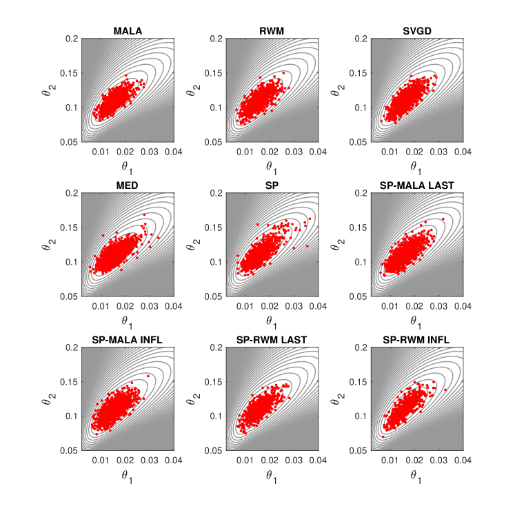
Figure S1: Quantisation in the IGARCH experiment. For the IGARCH experiment, we display point sets of size $n=1000$ produced by each of MCMC, SP, MED, SVGD and SP-MCMC, as described in Section 4.3 and Appendix A.6.3.

A.6.4 Performance of the Preconditioner Kernel

The performance of the preconditioner kernel in (6) was explored by comparing the default case $\Lambda=I$ (i.e. where a preconditioner is not used) to the case where $\Lambda$ is estimated based on a short run of MCMC. For this comparison we first considered the IGARCH experiment described in Sec. 4.3. This is expected to prove to be a challenging example for a preconditioner, in the sense the posterior is already unimodal and fairly well-conditioned. To test this hypothesis, the experiment reported in the main text was performed for both selections of $\Lambda$ and the results are reported in Fig. S2 (left). It can indeed be seen that the use of a preconditioner does not lead to a gain in performance in this case; however, and importantly, performance does not get worse as a result of the preconditioner being used.

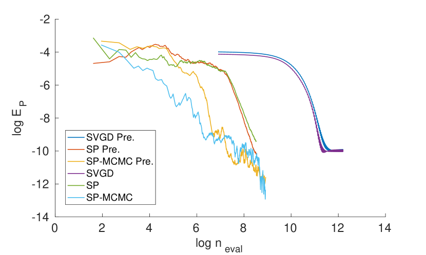
(a) IGARCH Model

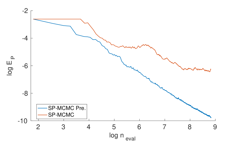
(b) Toy Model

Figure S2: Assessing the contribution of the preconditioner kernel. For the IGARCH experiment (left), we compared the performance of SP, SVGD and SP-MCMC each with and without a preconditioner matrix $\Lambda$ being used. In addition, a toy model (right) was explored for which the natural scale of the state vector $x$ was not commensurate with the naive choice of preconditioner matrix $\Lambda=I$. As in Fig. 3 in the main text, each method produced an empirical measure $\frac{1}{n}\sum_{i=1}^{n}\delta_{x_{i}}$ whose distance to the target $P$ was quantified by the energy distance $E_{P}$. The computational cost was quantified by the number $n_{\text{eval}}$ of times either $\tilde{p}$ or its gradient were evaluated.

To explore a scenario where the preconditioner demonstrates a benefit, we considered a toy model $P=\mathcal{N}(0,\sigma^{2}I)$ with $\sigma=0.01$. In this case the naive choice of $\Lambda=I$ was compared to the proposed approach of taking $\Lambda$ to be a sample-based approximation to the covariance of $P$. It is seen in Fig. S2 (right) that the preconditioner kernel out-performed the naive choice of $\Lambda=I$ for this model, emphasising the need to ensure $\Lambda$ is commensurate with the scale of the state variable $x$ in general.

An important point is that there is in general a computational cost associated with building an appropriate preconditioner matrix $\Lambda$ as just described. This is not explicitly accounted for in the experimental results that we report (i.e. not included in the total $n_{\text{eval}}$). To address this point, and to demonstrate that SP-MCMC can prove to be effective in the absence of this computational overhead, we refer the reader to the ODE example in Secs. 4.4 and A.6.6, where a simple preconditioner matrix $\Lambda\propto I$ was used and strong results were nevertheless obtained.

A.6.5 Removal of “Bad” Points

In this section we explored the implications of Remark 3 in the main text, which proposed to remove “bad” points from the current point set. This can be motivated by analogous strategies, known as away steps, explored in the Frank-Wolfe literature (e.g. Lacoste-Julien & Jaggi, 2015; Freund et al., 2017). An approach was considered such that, if the current point set in SP-MCMC is $\{x_{i}\}_{i=1}^{j-1}$, then in addition to identifying a possible next point $x_{j}$, we also identify a “bad” point $x_{i^{*}}$ that minimises $D_{\mathcal{K}_{0},P}(\{x_{i}\}_{i=1}^{j-1}\setminus\{x_{i^{*}}\})$. Then we compare the two quantities

$$\Delta_{\text{good}} := D_{\mathcal{K}_{0},P}(\{x_{i}\}_{i=1}^{j-1})-D_{\mathcal{K}_{0},P}(\{x_{i}\}_{i=1}^{j})$$

$$\Delta_{\text{bad}} := D_{\mathcal{K}_{0},P}(\{x_{i}\}_{i=1}^{j-1})-D_{\mathcal{K}_{0},P}(\{x_{i}\}_{i=1}^{j-1}\setminus\{x_{i^{*}}\}).$$

If either $j=1$ or $\Delta_{\text{good}}>\Delta_{\text{bad}}$, then the new point $x_{j}$ is included in the point set, so that the updated point set is $\{x_{i}\}_{i=1}^{j}$. Otherwise we remove the “bad” point from the point set, so that the update point set is $\{x_{i}\}_{i=1}^{j-1}\setminus\{x_{i^{*}}\}$. As such, with this approach the iteration number of the SP-MCMC algorithm is no longer identical to the size of the point set and the computational cost required to obtain a size $n$ point set may be increased relative to vanilla SP-MCMC. However, it is possible that this approach can lead to improved performance at the quantisation task.

To empirically test this approach, we revisit the IGARCH experiment in Sec. 4.3 of the main text. The SP-MCMC method was implemented with the INFL criterion and with $m_{j}=5$, identical to the experiment shown in the main text. Results comparing the impact of removing “bad points” in the manner described above are shown in Fig. S3. Interestingly, this was not seen to work well because too frequently a point would be removed, leading to sets containing only a small number of points. To investigate further, we considered an alternative approach wherein the “current worst” point would occasionally be removed. Results are also depicted in Fig. S3, based on a “dropping” rate of 25%. This led to larger point sets and an improved performance as measured by $E_{P}$. However, neither strategy considered outperformed the default approach where points were never removed.

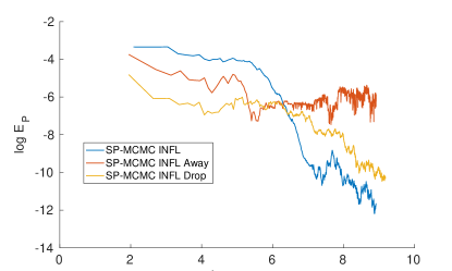
Figure S3: Assessing the benefit of removing “bad” points. For the IGARCH experiment, we compared the performance of SP-MCMC with and without away steps (“Away”) being used. In addition a simpler procedure, whereby the “current worst” point is occasionally dropped (“Drop”), was considered. As in Fig. 3 in the main text, each method produced an empirical measure $\frac{1}{n}\sum_{i=1}^{n}\delta_{x_{i}}$ whose distance to the target $P$ was quantified by the energy distance $E_{P}$. The computational cost was quantified by the number $n_{\text{eval}}$ of times either $\tilde{p}$ or its gradient were evaluated.

A.6.6 Goodwin Oscillator

The Goodwin oscillator (Goodwin, 1965) is a dynamical model of oscillatory enzymatic control. This kinetic model, specified by a system of $q$ ODEs, describes how a negative feedback loop between protein expression and mRNA transcription can induce oscillatory dynamics at a cellular level. In this work we considered Bayesian parameter estimation for two such models; a simple model with no intermediate protein species ($q=2$) and a more complex model with six intermediate protein species ($q=8$). The experimental protocol below follows that used in the earlier work of (Calderhead & Girolami, 2009; Oates et al., 2016).

The Goodwin oscillator with $q$ species is given by

$$\frac{\mathrm{d}u_{1}}{dt} = \frac{a_{1}}{1+a_{2}u_{q}^{\rho}}-\alpha u_{1}$$ (38)

$$\frac{\mathrm{d}u_{2}}{dt} = k_{1}u_{1}-\alpha u_{2}$$

$$\vdots$$

$$\frac{\mathrm{d}u_{q}}{dt} = k_{q-1}u_{q-1}-\alpha u_{q}.$$

The variable $u_{1}$ represents the concentration of mRNA and $u_{2}$ represents its corresponding protein product. The variables $u_{3},\dots,u_{q}$ represent intermediate protein species that facilitate a cascade of enzymatic activation leading, ultimately, to a negative feedback, via $u_{q}$, on the rate at which mRNA is transcribed. The Goodwin oscillator permits oscillatory solutions only when $\rho>8$. Following (Calderhead & Girolami, 2009; Oates et al., 2016) we set $\rho=10$ as a fixed parameter. The solution $u(t)$ of this dynamical system depends upon synthesis rate constants $a_{1}$, $k_{1},\dots,k_{q-1}$ and degradation rate constants $a_{2}$, $\alpha$. Thus the parameter vector $\theta=[a_{1},a_{2},k_{1},\dots,k_{q-1},\alpha]\in[0,\infty)^{q+2}$ and a $q$-variable Goodwin model has $d=q+2$ uncertain parameters to be inferred.

For this experiment we followed (Oates et al., 2016) and considered a realistic setting where only mRNA and protein product are observed, corresponding to $g(u)=[u_{1},u_{2}]$. For the initial condition we took $u_{0}=[0,\dots,0]$ and for the measurement noise we took $\sigma=0.1$, both considered known and fixed. Data $\{y_{i}\}_{i=1}^{40}$ were generated using $a_{1}=1$, $a_{2}=3$, $k_{1}=2$, $k_{2},\dots,k_{q-1}=1$, $\alpha=0.5$, as in (Oates et al., 2016). Thus the likelihood function for these data has the Gaussian form

$$p(y|\theta) = \frac{1}{(2\pi\sigma^{2})^{20}}\exp\left(-\frac{1}{2\sigma^{2}}\sum_{i=1}^{40}\|y_{i}-g(u(t_{i}))\|_{2}^{2}\right).$$

To set up the Bayesian inferential framework, each parameter $\theta_{i}$ was assigned an independent $\Gamma(2,1)$ prior belief. Note that, in order to ensure that boundary conditions in Sec. 2.1 were satisfied, we subsequently worked with the log-transformed parameters $x=\log(\theta)\in\mathbb{R}^{d}$, identifying the posterior distribution of $x$ with the target $P$ in our assessment.

In order to obtain the gradient $\nabla\log\tilde{p}$ it is required to differentiate the solution $u(t_{i})$ of the ODE with respect to the parameters $x$ at each time point $i\in\{1,\dots,40\}$. Of course, from the chain rule it is sufficient in what follows to consider differentiation of $u(t_{i})$ with respect to $\theta$. To this end, define the sensitivities $S_{j,k}^{i}:=\frac{\partial u_{k}}{\partial\theta_{i}}(t_{j})$, and note that these satisfy

$$\frac{\mathrm{d}}{\mathrm{d}t}S_{j,k}^{i}=\frac{\partial f_{k}}{\partial\theta_{i}}+\sum_{l=1}^{q}\frac{\partial f_{k}}{\partial u_{l}}S_{j,l}^{i}$$ (39)

where $\frac{\partial u_{k}}{\partial\theta_{i}}=0$ at $t=0$. The sensitivities can therefore be numerically computed by augmenting the state vector $u$ of the original ODE to include the $S_{j,k}^{i}$. In this work the ode45 solver in MATLAB was used to numerically solve this augmented ODE.

For SP-MCMC, we found that construction of a suitable preconditioner matrix $\Lambda$ was challenging due to the computational cost associated with each forward-solve of the ODE. To this end, we simply selected $\Lambda=0.3I$ for the case $d=4$ and $\Lambda=0.15I$ for the case $d=10$. The same kernel $k$, with this choice of $\Lambda$, was employed for each of SP, SP-MCMC and SVGD.

SP and MED were each implemented based on the same adaptive Monte Carlo search procedure described above in Alg. 1. To ensure a fair comparison, in each case the number of search points was taken equal to $m_{j}$, the length of the Markov chain used in SP-MCMC. The methods were run to produce a point set of size $n=300$.

For SVGD the size $n$ of the point set must be pre-specified. In order to ensure a fair comparison with SP-MCMC we considered a point set of size $n=300$, which is identical to the size of point set that are untimately produced by SP-MCMC during the course of this experiment. The step size $\epsilon$ was hand-tuned to optimise the performance of SVGD in our experiment. To initialise SVGD, a point set was drawn independently at random from $\text{Uniform}(\theta^{*}-0.5\times 1,\theta^{*}+0.5\times 1)$, where $1=[1,\dots,1]$ where $\theta^{*}$ is the data-generating value of the parameter vector. The step-size $\epsilon$ for SVGD was set using Adagrad, as in (Liu & Wang, 2016), with master step size $0.005$ and momentum $0.9$.

References

- Abramowitz & Stegun (1972) Abramowitz, M. and Stegun, I. A. Handbook of Mathematical Functions. Dover, 1972.
- Bach et al. (2012) Bach, F., Lacoste-Julien, S., and Obozinski, G. On the equivalence between herding and conditional gradient algorithms. In Proceedings of the International Conference on Machine Learning, pp. 1355–1362, 2012.
- Baringhaus & Franz (2004) Baringhaus, L. and Franz, C. On a new multivariate two-sample test. Journal of Multivariate Analysis, 88(1):190–206, 2004.
- Barp et al. (2018a) Barp, A., Briol, F.-X., Kennedy, A. D., and Girolami, M. Geometry and dynamics for Markov chain Monte Carlo. Annual Reviews in Statistics and its Applications, 5:451–471, 2018a.
- Barp et al. (2018b) Barp, A., Oates, C., Porcu, E., and M, G. A Riemannian-Stein kernel method. arXiv:1810.04946, 2018b.
- Berlinet & Thomas-Agnan (2004) Berlinet, A. and Thomas-Agnan, C. Reproducing Kernel Hilbert Spaces in Probability and Statistics. Springer Science & Business Media, New York, 2004.
- Calderhead & Girolami (2009) Calderhead, B. and Girolami, M. Estimating Bayes factors via thermodynamic integration and population MCMC. Computational Statistics & Data Analysis, 53(12):4028–4045, 2009.
- Chen et al. (2018a) Chen, C., Zhang, R., Wang, W., Li, B., and Chen, L. A unified particle-optimization framework for scalable Bayesian sampling. In Proceedings of the 34th Conference on Uncertainty in Artificial Intelligence, 2018a.
- Chen et al. (2018b) Chen, W. Y., Mackey, L., Gorham, J., Briol, F.-X., and Oates, C. J. Stein points. In Proceedings of the 35th International Conference on Machine Learning, volume 80, pp. 843–852. PMLR, 2018b.
- Chen et al. (2010) Chen, Y., Welling, M., and Smola, A. Super-samples from kernel herding. In Proceedings of the Conference on Uncertainty in Artificial Intelligence, 2010.
- Chwialkowski et al. (2016) Chwialkowski, K., Strathmann, H., and Gretton, A. A kernel test of goodness of fit. In Proceedings of the 33rd International Conference on Machine Learning, pp. 2606–2615, 2016.
- De Marchi et al. (2005) De Marchi, S., Schaback, R., and Wendland, H. Near-optimal data-independent point locations for radial basis function interpolation. Advances in Computational Mathematics, 23(3):317–330, 2005.
- Detommaso et al. (2018) Detommaso, G., Cui, T., Spantini, A., Marzouk, Y., and Scheichl, R. A Stein variational Newton method. In Advances in Neural Information Processing Systems 31, pp. 9187–9197, 2018.
- Dick & Pillichshammer (2010) Dick, J. and Pillichshammer, F. Digital Nets and Sequences - Discrepancy Theory and Quasi-Monte Carlo Integration. Cambridge University Press, 2010.
- Eberle (2016) Eberle, A. Reflection couplings and contraction rates for diffusions. Probability Theory and Related Fields, 166(3-4):851–886, 2016.
- Freund et al. (2017) Freund, R. M., Grigas, P., and Mazumder, R. An extended Frank–Wolfe method with “in-face” directions, and its application to low-rank matrix completion. SIAM Journal on Optimization, 27(1):319–346, 2017.
- Frogner & Poggio (2018) Frogner, C. and Poggio, T. Approximate inference with Wasserstein gradient flows. arXiv:1806.04542, 2018.
- Futami et al. (2018) Futami, F., Cui, Z., Sato, I., and Sugiyama, M. Frank-Wolfe Stein sampling. arXiv:1805.07912, 2018.
- Girolami & Calderhead (2011) Girolami, M. and Calderhead, B. Riemann manifold Langevin and Hamiltonian Monte Carlo methods. Journal of the Royal Statistical Society. Series B, 73(2):123–214, 2011.
- Goodwin (1965) Goodwin, B. C. Oscillatory behavior in enzymatic control process. Advances in Enzyme Regulation, 3:318–356, 1965.
- Gorham & Mackey (2015) Gorham, J. and Mackey, L. Measuring sample quality with Stein’s method. In Advances in Neural Information Processing Systems, pp. 226–234, 2015.
- Gorham & Mackey (2017) Gorham, J. and Mackey, L. Measuring sample quality with kernels. In Proceedings of the 34th International Conference on Machine Learning, pp. 1292–1301, 2017.
- Gorham et al. (2019) Gorham, J., Duncan, A., Mackey, L., and Vollmer, S. Measuring sample quality with diffusions. Annals of Applied Probability, 2019. In press.
- Graf & Luschgy (2007) Graf, S. and Luschgy, H. Foundations of Quantization for Probability Distributions. Springer, 2007.
- Gretton et al. (2006) Gretton, A., Borgwardt, K. M., Rasch, M. J., Schölkopf, B., and Smola, A. J. A kernel method for the two-sample-problem. In Advances in Neural Information Processing Systems, pp. 513–520, 2006.
- Hu et al. (2018) Hu, T., Chen, Z., Sun, H., Bai, J., Ye, M., and Cheng, G. Stein neural sampler. arXiv:1810.03545, 2018.
- Huggins & Mackey (2018) Huggins, J. and Mackey, L. Random feature Stein discrepancies. In Advances in Neural Information Processing Systems 31, pp. 1903–1913. 2018.
- Jitkrittum et al. (2017) Jitkrittum, W., Xu, W., Szabo, Z., Fukumizu, K., and Gretton, A. A linear-time kernel goodness-of-fit test. In Advances in Neural Information Processing Systems, pp. 261–270, 2017.
- Joseph et al. (2015) Joseph, V. R., Dasgupta, T., Tuo, R., and Wu, C. Sequential exploration of complex surfaces using minimum energy designs. Technometrics, 57(1):64–74, 2015.
- Joseph et al. (2018) Joseph, V. R., Wang, D., Gu, L., Lyu, S., and Tuo, R. Deterministic sampling of expensive posteriors using minimum energy designs. Technometrics, 2018. To appear.
- Lacoste-Julien & Jaggi (2015) Lacoste-Julien, S. and Jaggi, M. On the global linear convergence of Frank-Wolfe optimization variants. In Advances in Neural Information Processing Systems, pp. 496–504, 2015.
- Lacoste-Julien et al. (2015) Lacoste-Julien, S., Lindsten, F., and Bach, F. Sequential kernel herding: Frank-Wolfe optimization for particle filtering. In Proceedings of the 18th International Conference on Artificial Intelligence and Statistics, pp. 544–552, 2015.
- Li et al. (2019) Li, L., Li, Y., Liu, J., Liu, Z., and Lu, J. A stochastic version of Stein variational gradient descent for efficient sampling. arXiv:1902.03394, 2019.
- Liu & Zhu (2018) Liu, C. and Zhu, J. Riemannian Stein variational gradient descent for Bayesian inference. In Thirty-Second AAAI Conference on Artificial Intelligence, 2018.
- Liu (2017) Liu, Q. Stein variational gradient descent as gradient flow. In Advances in Neural Information Processing Systems, pp. 3118–3126, 2017.
- Liu & Wang (2016) Liu, Q. and Wang, D. Stein variational gradient descent: A general purpose Bayesian inference algorithm. In Advances in Neural Information Processing Systems, pp. 2378–2386, 2016.
- Liu & Wang (2018) Liu, Q. and Wang, D. Stein variational gradient descent as moment matching. In Advances in Neural Information Processing Systems, pp. 8868–8877, 2018.
- Liu et al. (2016) Liu, Q., Lee, J. D., and Jordan, M. I. A kernelized Stein discrepancy for goodness-of-fit tests and model evaluation. In Proceedings of the 33rd International Conference on Machine Learning, pp. 276–284, 2016.
- Lu et al. (2018) Lu, J., Lu, Y., and Nolen, J. Scaling limit of the Stein variational gradient descent: The mean field regime. SIAM Journal on Mathematical Analysis, 2018. To appear.
- Mak & Joseph (2018) Mak, S. and Joseph, V. R. Support points. Annals of Statistics, 46(6A):2562–2592, 2018.
- Metropolis et al. (1953) Metropolis, N., Rosenbluth, A. W., Rosenbluth, M. N., Teller, A. H., and Teller, E. Equation of state calculations by fast computing machines. The Journal of Chemical Physics, 21(6):1087–1092, 1953.
- Meyn & Tweedie (2012) Meyn, S. and Tweedie, R. Markov Chains and Stochastic Stability. Springer Science & Business Media., 2012.
- Muller (1997) Muller, A. Integral probability metrics and their generating classes of functions. Advances in Applied Probability, 29(2):429–443, 1997.
- Nelder & Mead (1965) Nelder, J. and Mead, R. A simplex method for function minimization. The Computer Journal, 7(4):308–313, 1965.
- Oates et al. (2016) Oates, C. J., Papamarkou, T., and Girolami, M. The controlled thermodynamic integral for Bayesian model evidence evaluation. Journal of the American Statistical Association, 111(514):634–645, 2016.
- Oates et al. (2017) Oates, C. J., Girolami, M., and Chopin, N. Control functionals for Monte Carlo integration. Journal of the Royal Statistical Society, Series B, 79(3):695–718, 2017.
- Parno (2015) Parno, M. D. Transport maps for accelerated Bayesian computation. PhD thesis, Massachusetts Institute of Technology, 2015.
- Robert & Casella (2004) Robert, C. and Casella, G. Monte Carlo Statistical Methods. Springer, 2004.
- Roberts & Rosenthal (2001) Roberts, G. O. and Rosenthal, J. S. Optimal scaling for various Metropolis-Hastings algorithms. Statistical Science, 16(4):351–367, 2001.
- Roberts & Tweedie (1996) Roberts, G. O. and Tweedie, R. L. Exponential convergence of Langevin distributions and their discrete approximations. Bernoulli, 2(4):341–363, 1996.
- Roshan Joseph et al. (2015) Roshan Joseph, V., Dasgupta, T., Tuo, R., and Jeff Wu, C. F. Sequential exploration of complex surfaces using minimum energy designs. Technometrics, 57(1):64–74, 2015.
- Santin & Haasdonk (2017) Santin, G. and Haasdonk, B. Convergence rate of the data-independent P-greedy algorithm in kernel-based approximation. Dolomites Research Notes on Approximation, 10, 2017.
- Sejdinovic et al. (2013) Sejdinovic, D., Sriperumbudur, B., Gretton, A., and Fukumizu, K. Equivalence of distance-based and rkhs-based statistics in hypothesis testing. Annals of Statistics, pp. 2263–2291, 2013.
- Stein (1972) Stein, C. A bound for the error in the normal approximation to the distribution of a sum of dependent random variables. In Proceedings of 6th Berkeley Symposium on Mathematical Statistics and Probability, pp. 583–602. University of California Press, 1972.
- Székely & Rizzo (2004) Székely, G. and Rizzo, M. Testing for equal distributions in high dimension. InterStat, 5(16.10):1249–1272, 2004.
- Taylor (2011) Taylor, S. J. Asset Price Dynamics, Volatility, and Prediction. Princeton University Press, 2011.
- Wang et al. (2018) Wang, D., Zeng, Z., and Liu, Q. Stein variational message passing for continuous graphical models. In Proceedings of the 35th International Conference on Machine Learning, PMLR 80, pp. 5219–5227, 2018.
- Zhang et al. (2018) Zhang, R., Chen, C., Li, C., and Carin, L. Policy optimization as Wasserstein gradient flows. In Proceedings of the 35th International Conference on Machine Learning, pp. 5737–5746, 2018.
- Zhuo et al. (2018) Zhuo, J., Liu, C., Shi, J., Zhu, J., Chen, N., and Zhang, B. Message passing Stein variational gradient descent. In Proceedings of the 35th International Conference on Machine Learning, PMLR 80:6013-6022, 2018.