Stability of steady states and bifurcation to traveling waves in a free boundary model of cell motility

Abstract

We introduce a two-dimensional coupled Hele-Shaw/ Keller-Segel type free boundary model for motility of eukaryotic cells on substrates. The key ingredients of this model are the Darcy law for overdamped motion of the cytoskeleton (active) gel and Hele-Shaw type boundary conditions (Young-Laplace equation for pressure and continuity of velocities). We first show that radially symmetric steady state solutions become unstable and bifurcate to traveling wave solutions. Next we establish linear and nonlinear stability of the steady states. We show that linear stability analysis is inconclusive for both steady states and traveling waves. Therefore we use invariance properties to prove nonlinear stability of steady states.

1 Introduction

Motion of living cells has been the subject of extensive studies in biology, soft-matter physics and more recently in mathematics. Living cells are primarily driven by cytoskeleton gel dynamics. The study of cytoskeleton gels led to a recent development of the so-called “Active gel physics”, see [5].

The key element of this motion is cell polarity, which enables cells to carry out specialized functions and therefore is a fundamental issue in cell biology. Also motion of specific cells such as keratocytes in the cornea is of medical relevance as they are involved, e.g., in wound healing after eye surgery or injuries. Moreover keratocytes are perfect for experiments and modeling since they are naturally found on flat surfaces, which allows capturing the main features of their motion by spatially two dimensional models. The typical modes of motion of keratocytes in both cornea and fishscales are rest (no movement at all) or steady motion with fixed shape, speed, and direction [14, 22]. That is why it is important to study the steady states and traveling waves that describe resting cells and steadily moving cells respectively.

The two leading mechanisms of cell motion are protrusion generated by polymerization of actin filaments (more precisely, filamentous actin or F-actin) and contraction due to myosin motors [14]. Our goal is to study the contraction driven cell motion when polymerization is negligible since it is balanced by depolymerization (complementary work on polymerization without myosin contraction, see [12], [16]). To this end we introduce and investigate a 2D model with free boundary that generalizes 1D Keller-Segel type free boundary model from [19], [20]. Even though the boundary in 1D is simply two points, our analysis shows that several key qualitative properties established in [19], [20] are also observed in 2D. However, the transition from 1D to 2D requires addressing new issues such as modeling and analysis of evolution of the domain shape. For instance, the problem on a moving interval of variable length (1D domain with free boundary) is reduced to a problem on a fixed interval via a linear change of variable, whereas in 2D case such a reduction requires a much more sophisticated nonlinear change of variables.

Two-dimensional active gel models with free boundary were introduced in, e.g., [22], [7], [4]. The problems in [7], [4] model the polymerization driven cell motion when myosin contraction is dominated by polymerization, which naturally complements present work. Although the model from [4] looks similar to the classical Hele-Shaw model, the two are different in some fundamental aspects such as presence of persistent motion modeled by traveling wave solution. More recently a 2D model of the intracellular dynamics with fixed cell shape as a disc was introduced and analyzed numerically analytically in [13].

A free boundary 2D model introduced and analyzed numerically in [22] accounts for both polymerization and myosin contraction. This model was studied analytically in [2] where the traveling wave solutions were established. It was also shown in [2] that this model reduces to the Keller-Segel system in a free boundary setting. This system in fixed domains appears in various chemotaxis models and it has been extensively studied in mathematical literature due to the finite time blow-up phenomenon caused by the cross-diffusion term ([23],p.1903) in dimensions 2 and higher. The fact that the minimal model of contraction driven motility reduces to a Keller-Segel system with free boundaries was first realized in [19] where the corresponding traveling wave solutions were analyzed in the simplest 1D setting.

While in the model [22] the kinematic condition at the free boundary contains curvature, in present work we assume continuity of velocities of the gel and the membrane (boundary) as in 1D model [19], [20]) but adapt the Young-Laplace equation for the pressure on the boundary as usually done in Hele-Shaw model and has no analog in 1D.

Our objective is analysis of the coupled Hele-Shaw/Keller-Segel model. Specifically, we are interested in existence and stability of its special solutions such as steady states and traveling waves, which are important for understanding cell motility. While the existence of radially symmetric steady states is straightforward, their nonlinear stability analysis is highly non-trivial. Indeed, we first perform the linear stability analysis around radial steady states and show that the linearized operator has zero eigenvalue of multiplicity 2. The corresponding two eigenvectors appear since these steady states are a continuum family parametrized by their centers (shift invariance) and radii. Thus, the linear stability analysis is inconclusive. For nonlinear stability we need to control the component of the solution corresponding to the both eigenvectors. For the first eigenvector we use factorization in shifts for the linearized problem, whereas for the second one we use conservation of total myosin mass in place a Lyapunov function, which is a standard tool in proof of nonlinear stability (it is known that establishing Lyapunov function in free boundary problems is quite difficult). Another challenge in the proof of nonlinear stability of steady states can be described as follows. The problem with free boundary is reduced to a problem in a fixed domain (a disk). For classical Hele-Shaw problem, this is done by conformal maps since the pressure is harmonic and therefore the PDE is conformally invariant [8], [4]. However, the pressure in our problem, see (7)-(11), is not harmonic due to coupling with myosin density. Similar difficulty arises in tumor growth free boundary problems, see, e.g., [11], [1], where it is dealt with by applying the Hanzawa transform. However, the Hanzawa transform can not be used in problem (7)–(11) due to the Neumann condition (11). Indeed, this transform does not preserve normal derivative leading to a time dependent boundary condition in a parabolic equation which is hard to deal with. That is why we construct another transform which preserves normal derivative but is more sophisticated. Reduction of the PDEs to the fixed disk, with the help of aforementioned transform leads to new nonlinear terms, see $f_{i}$ and $g_{i}$, $i=1,2$ in (113)–(118). These terms contain high order derivatives and one needs to establish optimal regularity and decay results for linearized problem to employ fixed point argument for existence of solutions and their stability. To this end we establish global regularity properties for our free boundary problems (for general geometric regularity results in free boundary problems see [6]).

Finally, we note that free boundary problems in cell motility are closely related to the free boundary problems in tumor growth models. The key differences are that in the letter models the area of domain undergoes significant changes and there is no persistent motion (see, e.g., [10], [18], and [15]).

The paper is organized as follows. In Section 2 we introduce a 2D model of active gel that is a free boundary problem with Keller-Segel PDEs. In Section 3 we consider linearization around radially symmetric steady states and introduce a function of geometrical and physical parameters (the domain radius, adhesion strength and myosin density). Theorem 3.3 establishes a critical value of this function that separates stability and instability regimes. In Section 4 we show that at this critical value bifurcation of the steady states occurs and traveling wave solutions appear, as described in Theorem 4.1. These solutions model persistent motion which is the signature feature of cytoskeleton gels motility. Section 5 is devoted to linear stability analysis of the traveling wave solutions which yields stability up to a slow center manifold. Finally, Theorem 6.1 in Section 6 establishes nonlinear stability of steady states for subcritical values of the parameters.

Acknowledgments. VR is grateful to PSU Center for Mathematics of Living and Mimetic Matter, and to PSU Center for Interdisciplinary Mathematics for support of his two stays at Penn State. His travel was also supported by NSF grant DMS-1405769. We thank our colleagues I. Aronson, J.-F. Joanny, N. Meunier, A. Mogilner, J. Prost and L. Truskinovsky for useful discussions and suggestions on the model. We also express our gratitude to the members of the L. Berlyand’s PSU research team, R. Creese, J. King, M. Potomkin, and A. Saftsten, for careful reading and help in the preparation of the manuscript.

2 The model

We consider a 2D model of motion of an active gel drop which occupies a domain $\Omega(t)$ with free boundary. The flow of the acto-myosin network inside the domain $\Omega(t)$ is described by the velocity field $u$. In the adhesion dominated regime (overdamped flow) [7] , [4] $u$ obeys the Darcy’s law

$$-\nabla p=\zeta u\quad\text{in}\ \Omega(t),$$ (1)

where $-p$ stands for the scalar stress ($p$ is the pressure) and $\zeta$ is the constant effective adhesion drag coefficient. We consider compressible gel (the actomyosin network is a compressible fluid, incompressible cytoplasm fluid can be squeezed easily into the dorsal direction in the cell [17]). The main modeling assumption of this work is the following constitutive law for the scalar stress $-p$

$$-p=\mu{\rm div}u+km-p_{\rm h},$$ (2)

where $\mu{\rm div}u$ is the hydrodynamic stress ($\mu$ being the effective bulk viscosity of the gel), the middle term $km$ is the active component of the stress which is proportional to the density $m=m(x,y,t)>0$ of myosin motors with a constant contractility coefficient $k>0$, $p_{\rm h}$ is the constant homeostatic pressure. Throughout this work we assume that the effective bulk viscosity and the contractility coefficient $k$ in (2) are scaled to $\mu=1$, $k=1$. We prescribe the following condition on the boundary

$$p+p_{\rm e}=\gamma\kappa\quad\text{on}\ \partial\Omega(t),$$ (3)

known as the Young-Laplace equation, where $\kappa$ denotes the curvature, $\gamma>0$ is a constant coefficient and $p_{\rm e}$ is the effective traction which describes the mechanism of approximate conservation of the area due to the membrane-cortex tension. The traction $p_{\rm e}$ generalizes the one-dimensional nonlocal spring condition introduced in [19], [20], see a more recent work [21] which also introduces the cell volume regulating homeostatic pressure , and we similarly assume the simple linear dependence $p_{\rm e}=-k_{\rm e}|\Omega|$ of $p_{\rm e}$ on the area $|\Omega|$, where $k_{\rm e}$ is the stiffness coefficient. The evolution of motor density is described by the advection-diffusion equation

$$\partial_{t}m=\Delta m-{\rm div}(um)\quad\text{in}\ \Omega(t)$$ (4)

and no flux boundary condition in moving domain

$$\partial_{\nu}m=((u\cdot\nu)-V_{\nu})m\quad\text{on}\ \partial\Omega(t),$$ (5)

$\nu$ stands for the outward pointing normal vector and $V_{\nu}$ is the normal velocity of the domain $\Omega(t)$. Finally, we assume continuity of velocities on the boundary

$$V_{\nu}=(u\cdot\nu),$$ (6)

so that (5) becomes the standard Neumann condition. Combining (1)–(6) yields a closed set of equations that forms a model of cell motility investigated in this work.

It is convenient to introduce the potential for the velocity field $u$ using (1):

$$u=\nabla\phi=-\nabla\frac{1}{\zeta}p$$

and rewrite problem (1)–(6) in the form

$$\Delta\phi+m=\zeta\phi+p_{\rm eff}(|\Omega(t)|)\quad\text{in}\ \Omega(t),$$ (7)

$$\zeta\phi=-\gamma\kappa\quad\text{on}\ \partial\Omega(t),$$ (8)

$$V_{\nu}=\partial_{\nu}\phi\quad\text{on}\ \partial\Omega(t),$$ (9)

$$\partial_{t}m=\Delta m-{\rm div}(m\nabla\phi),\quad\text{in}\ \Omega(t),$$ (10)

$$\partial_{\nu}m=0\quad\text{on}\ \partial\Omega(t),$$ (11)

where we introduce the notation $p_{\rm eff}:=p_{\rm h}+p_{\rm e}=p_{\rm h}-k_{\rm e}|\Omega(t)|$. We assume that the area $|\Omega(t)|$ is such that

$$p_{\rm eff}=p_{\rm eff}(|\Omega(t)|)>0.$$ (12)

Moreover, we consider the stiffness coefficient $k_{\rm e}$ to be sufficiently large so that it penalizes changes of the area. For instance, it prevents from shrinking of $\Omega$ to a point or from infinite expanding. Precise lower bound on $k_{\rm e}=-p_{\rm eff}^{\prime}$ is given in (31), see also Remark 3.5.

Remark 2.1.

We view problem (7)–(11) as an evolution problem with respect to two unknowns $m(x,y,t)$ and $\Omega(t)$, while the potential $\phi(x,y,t)$ is considered as an additional unknown function defining evolution of the free boundary. Indeed, for given $\Omega(t)$ and $m(x,y,t)$ the function $\phi(x,y,t)$ is obtained as the unique solution of the elliptic problem (7)–(8), and its normal derivative $\partial_{\nu}\phi$ defines normal velocity of the domain due to (9). Problem (7)–(11) is supplied with initial conditions for $m$ and $\Omega$ and it is natural not to include the unknown $\phi$ into the phase space of this evolution problem but rather in the definition of the operator governing the semi-group in this phase space that defines the evolution of $m$ and $\Omega$.

In what follows we assume for simplicity that problem (7)–(11) is symmetric with respect to $x$-axis. Specifically we assume symmetry of the initial data, domain $\Omega(0)$ and $m(x,y,t=0)$ which is preserved for $t>0$.

3 Linear stability analysis of radially symmetric steady states

Problem (7)–(11) possesses a family of radially symmetric solutions with both $\phi$ and $m$ being constant. For a given radius $R>0$ the constant solution, $\phi=\phi_{0}$ and $m=m_{0}$, is obtained from (8) and (7) in the domain $\Omega(t)=B_{R}$ and it is verified by the direct substitution ($B_{R}$ is the disk with radius $R$):

$$\Omega=B_{R},\quad m_{0}:=-\gamma/R+p_{\rm eff}(\pi R^{2}),$$ (13)

$$\phi_{0}=-\gamma/(\zeta R).$$

It is convenient to use polar coordinate system $(r,\varphi)$ whose origin is moving with the domain,

$$\Omega(t)=\{(x=r\cos\varphi+X_{c}(t),y=r\sin\varphi);0\leq r<R+\rho(\varphi,t)\},$$ (14)

where $X_{c}(t)$ is an approximation of $\tilde{X_{c}}(t)$, the $x$ coordinate of the center of mass of $\partial\Omega$, and $\rho(\varphi,t)$ satisfies the following orthogonality condition that eliminates infinitesimal shifts

$$\int_{-\pi}^{\pi}\rho(\varphi,t)\cos\varphi d\varphi=0,\quad\text{ for all }t>0.$$ (15)

Indeed, formula (15) is a linearization of the the $x$ coordinate of the center of mass $\tilde{X}_{c}(t)$ of $\partial\Omega$:

$$0 = \frac{1}{|\partial\Omega|}\int\limits_{\partial\Omega}x\,d\sigma-\tilde{X}_{c}$$ (16)

$$= \frac{1}{|\partial\Omega|}\int_{\partial\Omega}(x-\tilde{X}_{c})\,\text{d}\sigma$$

$$= \frac{1}{|\partial\Omega|}\int_{-\pi}^{\pi}(R+\rho(\varphi,t))\cos\varphi\sqrt{(R+\rho(\varphi,t))^{2}+(\rho^{\prime}_{\varphi})^{2}}d\varphi$$

$$= \frac{1}{\pi}\int_{-\pi}^{\pi}\rho(\varphi,t)\,\cos(\varphi)\,d\varphi+O(\rho^{2}).$$

Here $\sigma$ denotes the arc length.

Linearizing problem (7)–(11) around the radially symmetric steady state (for $m_{0}$ from (13) and $\Omega(t)=B_{R}$) we get the following system

$$\partial_{t}\rho+\dot{X}_{c}\cos\varphi=\partial_{r}\phi\quad\text{on}\ \partial B_{R},$$ (17)

$$\Delta\phi+m=\zeta\phi+p_{\rm eff}^{\prime}(\pi R^{2})R\int_{-\pi}^{\pi}\rho(\varphi)d\varphi\quad\text{in}\ B_{R},$$ (18)

$$\phi=\frac{\gamma}{R^{2}\zeta}(\rho^{\prime\prime}+\rho)\quad\text{on}\ \partial B_{R},$$ (19)

$$\partial_{t}{m}=\Delta{m}-m_{0}\Delta{\phi}\quad\text{in}\ B_{R},\quad\partial_{r}m=0\quad\text{on}\ \partial B_{R},$$ (20)

the integral term in (18) appears due to linearization of the term $p_{\rm eff}(|\Omega|)$ in (7), $\rho^{\prime\prime}$ denotes $\partial_{\varphi}^{2}\rho$.

In operator form system (17)–(20) reads

$$\frac{d}{dt}U=\mathcal{A}U,$$

where $U=(m,\rho)$ and $\mathcal{A}$ is the following operator

$$\mathcal{A}:\left[\begin{array}[]{c}m\\ \rho\end{array}\right]\mapsto\left[\begin{array}[]{c}\Delta m-m_{0}\Delta\phi\\ \partial_{r}\phi-\frac{\cos\varphi}{\pi}\int_{-\pi}^{\pi}\partial_{r}\phi\cos\tilde{\varphi}\,d\tilde{\varphi}\end{array}\right],$$ (21)

where $\phi$ solves the time independent problem (18)–(19) for given $m$ and $\rho$. This operator is considered on pairs $U=(m,\rho)$ such that $m\in H^{2}(B_{R})$ and $\partial_{r}m=0$ on $\partial B_{R}$, $\rho\in H^{4}(-\pi,\pi)$ and $\rho$ is an even $2\pi$-periodic function. The integral term in (21) appears when the orthogonality condition (15) is applied to (17). The study of well posedness of the linearized system (17)–(20) and its stability amounts to the spectral analysis of the operator $\mathcal{A}$.

Observe that due to radial symmetry of operator $\mathcal{A}$ as well as its symmetry with respect to $x$-axis, all eigenvectors of $\mathcal{A}$ are of the form $m=\hat{m}(r)\cos(n\varphi)$ and $\rho=\hat{\rho}\cos(n\varphi)$ for integer $n\geq 0$, and $\phi$, the solution of (18)–(19), is of the similar form: $\phi=\hat{\phi}(r)\cos(n\varphi)$. The eigenvalue problem for operator $\mathcal{A}$ is:

$$\lambda m = \Delta m-m_{0}\Delta\phi\text{ in }B_{R},$$ (22)

$$\lambda\rho = (1-\delta_{n1})\partial_{r}\phi\text{ on }\partial B_{R},$$ (23)

$$-\Delta\phi+\zeta\phi = -m-2\pi p_{\rm eff}^{\prime}(\pi R^{2})R\,\hat{\rho}\,\delta_{n0}\text{ in }B_{R},$$ (24)

$$\phi = -\dfrac{\gamma(n^{2}-1)}{R^{2}\zeta}\hat{\rho}\text{ on }\partial B_{R},$$ (25)

$$\partial_{r}m = 0\text{ on }\partial B_{R},$$ (26)

where $\delta_{nk}$ is the Kronecker delta.

Remark 3.1.

(i) The operator $\mathcal{A}$ has zero eigenvalue with an eigenvector $(m,\rho(\varphi))=(0,\cos\varphi)$. The eigenspace corresponding to eigenvalue 0 represents infinitesimal shifts of the reference solution $m=m_{0},\rho=0$ and $\Omega=B_{R}$. To see this, note that if $\Omega=B_{R}+\varepsilon(1,0)$ (i.e., $\Omega$ is $B_{R}$ shifted by $\varepsilon$ along $x$-axis), then in view of (14) $\rho(\varphi)=\varepsilon\cos\varphi+o(\varepsilon)$ for small $\varepsilon$. Moreover, since problem (7)–(11) is translational invariant, then any shift of the solution is also a solution. However, $(0,\varepsilon\cos\varphi)$ are eigenfunctions of operator $\mathcal{A}$ obtained from the linearization of the original problem, these eigenfunctions correspond to infinitesimal shifts, not exact shifts.

(ii) Yet another zero eigenvalue of the operator $\mathcal{A}$ is obtained by taking derivative of the family of steady states (13) with respect to the parameter $R$. The corresponding eigenvector is $m=\gamma/R+2\pi p_{\rm eff}^{\prime}(\pi R^{2})R$, $\rho=1$.

While the two aforementioned eigenvectors corresponding to zero eigenvalue are trivially obtained by taking derivatives of families of steady states in the parameters, the following Lemma describes all other possible eigenvectors corresponding to the zero eigenvalue.

Lemma 3.2.

For $\zeta\geq m_{0}$ the operator $\mathcal{A}$ has zero eigenvalue corresponding to a nonconstant $m$ if and only if $m=m_{0}(\phi_{1}(r)-r)\cos\varphi$ and $\phi_{1}(r)$ solves

$$\frac{1}{r}(r\phi^{\prime}_{1}(r))^{\prime}-\frac{1}{r^{2}}\phi_{1}(r)+(m_{0}-\zeta)\phi_{1}(r)=m_{0}r\quad 0\leq r<R,\quad\phi_{1}(0)=0,\,\phi_{1}(R)=0.$$ (27)

and

$$\phi_{1}^{\prime}(R)=1.$$ (28)

Proof.

Set $\lambda=0$ in (22)-(26) and consider all integer $n\geq 0$.

If $n=0$, then $m=\hat{m}(r)$, $\phi=\hat{\phi}(r)$ and $\rho=\hat{\rho}$, and (22), (23) can be written as

$$\left\{\begin{array}[]{l}-\Delta(m-m_{0}\phi)=0,\\ ~{}~{}\partial_{r}(m-m_{0}\phi)|_{r=R}=0.\end{array}\right.$$

This implies that $m-m_{0}\phi=C_{1}$. Substituting $m=C_{1}+m_{0}\phi$ in (22) one obtains

$$\left\{\begin{array}[]{l}-\Delta\phi+(\zeta-m_{0})\phi=C_{2},\text{ in }B_{R},\\ ~{}~{}\partial_{r}\phi=0,\text{ on }\partial B_{R},\end{array}\right.$$ (29)

where $C_{2}=C_{1}-2\pi p^{\prime}_{h}(\pi R^{2})R^{3}\zeta\gamma^{-1}$. Since $\zeta\geq m_{0}$ one deduces that $\phi$ is constant Then $m$ is also constant, $m=C_{1}+m_{0}\phi$.

If $n=1$, then (22) implies that $u(r):=\hat{m}(r)-m_{0}\hat{\phi}(r)$ satisfies the following equation:

$$\frac{1}{r}(ru^{\prime})^{\prime}-\frac{1}{r^{2}}u=0,$$

therefore $u(r)=C_{3}r$. Thus, $\hat{m}=C_{3}r+m_{0}\hat{\phi}$. Substituting this representation for $\hat{m}$ into (24) we obtain,

$$\frac{1}{r}(r\hat{\phi}^{\prime})^{\prime}-\frac{1}{r^{2}}\hat{\phi}+(m_{0}-\zeta)\hat{\phi}=-C_{3}m_{0}r.$$ (30)

From continuity of $\phi$ at the origin we obtain that $\hat{\phi}(0)=0$. From (26) we obtain that $\tilde{\phi}^{\prime}(R)=-C_{3}$. Now taking $\phi_{1}(r):=\tilde{\phi}(r)/C_{3}$ we see that both (27) and (28) are satisfied.

If $n\geq 2$, we have

$$\frac{1}{r}(r\hat{\phi}^{\prime}(r))^{\prime}-\frac{n^{2}}{r^{2}}\hat{\phi}(r)+(m_{0}-\zeta)\hat{\phi}(r)=0\quad 0\leq r<R,\quad\hat{\phi}(0)=0,\,\hat{\phi}^{\prime}(R)=0.$$

The latter problem has only trivial solutions for $\zeta\geq m_{0}$. Then from (22) and (26) we deduce that $m=0$, while (25) yields $\hat{\rho}=0$.

Therefore, there exists a non-constant $m$, corresponding to the zero eigenvalue (that is, solution of (22)-(26) with $\lambda=0$) only in the case $n=1$, and in this case $\tilde{m}=m_{0}(\phi_{1}(r)-r)$ with $\phi_{1}(r)$ solving both (27) and (28).

∎

Theorem 3.3.

(Linear stability of steady states (13)). Assume that the myosin density $m_{0}$ is bounded above by the third eigenvalue of the operator $-\Delta$ in $B_{R}$ with the Neumann boundary condition on $\partial B_{R}$, also assume that $\zeta>m_{0}$ and $p_{\rm eff}^{\prime}(\pi R^{2})$ satisfies

$$p_{\rm eff}^{\prime}(\pi R^{2})\leq-\Bigl{(}\gamma/R+2m_{0}+\sqrt{2R\sqrt{\zeta}}m_{0}\Bigr{)}/(2\pi R^{2}).$$ (31)

Let $\phi_{1}$ be the solution of (27). Then

• if $\phi_{1}^{\prime}(R)<1$, then the operator $\mathcal{A}$ has zero eigenvalue $\lambda=0$ of multiplicity two, other eigenvalues have negative real parts,

• if $\phi_{1}^{\prime}(R)=1$, then the operator $\mathcal{A}$ has zero eigenvalue $\lambda=0$ of multiplicity three, other eigenvalues have negative real parts,

• if $\phi_{1}^{\prime}(R)>1$, then the operator $\mathcal{A}$ has a positive eigenvalue $\lambda>0$.

Remark 3.4.

It is well known that if linearized operator has zero eigenvalue, then linear spectral analysis is inconclusive for stability/instability of the underlying nonlinear system. As explained in Remark 3.1, operator $A$ always has zero eigenvalue with at least two eigenvectors (corresponding to infinitesimal shifts and the derivative of the family of steady states with respect to the radius. In Theorem 6.1, we establish stability in the case (i) in Theorem 3.3 by showing that the first eigenvector can be eliminated thanks to invariance of the problem (7)–(11) with respect to shifts and projection of the solution of (7)–(11) on the second eigenvector can be controlled due to conservation of myosin. In the case (iii) in Theorem 3.3 the linearized system is unstable implying instability of nonlinear system (7)–(11).

Remark 3.5.

Zero (radially symmetric) mode is responsible for the expansion and shrinking of the domain. The condition (31) assures that real part of the corresponding eigenvalue is negative, leading to stability with respect to infinitesimal expansion and shrinking.

Proof.

Thanks to radial symmetry of the problem (and our assumption about symmetry with respect to the $x$-axis) eigenvectors of $\mathcal{A}$ have the form $m=\hat{m}_{n}(r)\cos n\varphi$, $\rho=\hat{\rho}_{n}\cos n\varphi$. Consider first the case $n\geq 2$. In this case (18) takes form $\Delta\phi=\zeta\phi-m$, then we have

$$\lambda m=\Delta m+m_{0}m-m_{0}\zeta\phi.$$

Multply this equation by the complex conjugate $\overline{m}$ of $m$ and integrate over $B_{R}$ to find

$$\lambda\int_{B_{R}}|m|^{2}dxdy=-\int_{B_{R}}|\nabla m|^{2}dxdy+m_{0}\int_{B_{R}}|m|^{2}dxdy-m_{0}\zeta\int_{B_{R}}\phi\overline{m}dxdy.$$ (32)

Now multiply the equation $\overline{m}=\zeta\overline{\phi}-\Delta\overline{\phi}$ by $m_{0}\zeta\phi$ and integrate over $B_{R}$ to obtain the following representation for the last term in (32):

$$m_{0}\zeta\int_{B_{R}}\phi\overline{m}dxdy=m_{0}\zeta^{2}\int_{B_{R}}|\phi|^{2}dxdy+m_{0}\zeta\int_{B_{R}}|\nabla\phi|^{2}dxdy-m_{0}\zeta\int\phi{\partial_{r}\overline{\phi}}d\sigma$$

Since $\partial_{r}\overline{\phi}=\overline{\lambda}\overline{\rho}$ and by virtue of (19) $\overline{\rho}=\frac{R^{2}\zeta}{\gamma(1-n^{2})}\overline{\phi}$, equation (32) rewrites as

$$\lambda\int_{B_{R}}|m|^{2}dxdy+\overline{\lambda}\frac{m_{0}R^{2}\zeta^{2}}{\gamma(n^{2}-1)}\int|\phi|^{2}d\sigma= -\int_{B_{R}}|\nabla m|^{2}dxdy+m_{0}\int_{B_{R}}|m|^{2}dxdy$$

$$-m_{0}\zeta\int_{B_{R}}|\nabla\phi|^{2}dxdy-m_{0}\zeta^{2}\int_{B_{R}}|\phi|^{2}dxdy.$$

Note that for $n\geq 2$ the function $\hat{m}_{n}(r)\cos n\varphi$ is orthogonal to the first and second eigenfunctions of the operator $-\Delta$ in $B_{R}$ with the Neumann condition on $\partial B_{R}$, recall also that $m_{0}$ is bounded by the third eigenvalue. Then by Proposition 6.5 we have

$$\int_{B_{R}}|\nabla m|^{2}dxdy-m_{0}\int_{B_{R}}|m|^{2}dxdy\geq 0,$$

so that real part of $\lambda$ is negative.

Consider now the case $n=0$ which corresponds to radially symmetric eigenfunctions. Taking the derivative of steady states with respect to the parameter $R$ we obtain an eigenvector corresponding to zero eigenvalue. Let us show that other radially symmetric eigenvectors correspond to eigenvalues with negative real parts. It is convenient to change the unknown $\tilde{\phi}:=\phi+2\pi R\rho p_{\rm eff}^{\prime}(\pi R^{2})/\zeta$, then in view of (19) we have $\tilde{\phi}=\rho(\gamma/R^{2}+2\pi Rp_{\rm eff}^{\prime}(\pi R^{2}))/\zeta$ which in turn leads to the boundary condition

$$\partial_{r}\tilde{\phi}=\frac{\lambda\zeta}{\gamma/R^{2}+2\pi Rp_{\rm eff}^{\prime}(\pi R^{2})}\tilde{\phi}.$$

Then arguing as above we obtain the following relation

$$\lambda\int_{B_{R}}|m|^{2}dxdy-\overline{\lambda}\frac{m_{0}\zeta^{2}}{\gamma/R^{2}+2\pi Rp_{\rm eff}^{\prime}(\pi R^{2})} \int_{\partial B_{R}}|\tilde{\phi}|^{2}d\sigma=-\int_{B_{R}}|\nabla m|^{2}dxdy+m_{0}\int_{B_{R}}|m|^{2}dxdy$$ (33)

$$-m_{0}\zeta\int_{B_{R}}|\nabla\tilde{\phi}|^{2}dxdy-m_{0}\zeta^{2}\int_{B_{R}}|\tilde{\phi}|^{2}dxdy.$$

By Proposition 6.5 we have

$$\int_{B_{R}}|\nabla m|^{2}dxdy-m_{0}\int_{B_{R}}|m|^{2}dxdy\geq-m_{0}\pi R^{2}|\langle m\rangle|^{2}$$ (34)

because of the radial symmetry of $m$, where $\langle m\rangle$ denotes the mean value of $m$, $\langle m\rangle:=\frac{1}{\pi R^{2}}\int_{B_{R}}mdxdy$. Therefore real part of $\lambda$ is negative if $\langle m\rangle=0$. Thus we can normalize the eigenvector by setting

$$\langle m\rangle=1.$$ (35)

Assume also that $\lambda\not=0$. Then integrating the equation $\lambda m=\Delta m-m_{0}\Delta\tilde{\phi}$ we find

$$\langle m\rangle:=\frac{1}{\pi R^{2}}\int_{B_{R}}mdxdy=-\frac{m_{0}}{\lambda\pi R^{2}}\int_{\partial B_{R}}\partial_{r}\tilde{\phi}d\sigma=-\frac{2m_{0}\zeta}{{\gamma}/R+2\pi R^{2}p_{\rm eff}^{\prime}(\pi R^{2})}\tilde{\phi}(R).$$

Integrating also the equation $\Delta\tilde{\phi}+m=\zeta\tilde{\phi}$ we have

$$\zeta\langle\tilde{\phi}\rangle=\langle m\rangle+\frac{1}{\pi R^{2}}\int_{\partial B_{R}}\partial_{r}\tilde{\phi}d\sigma=(1-\lambda/m_{0})\langle m\rangle.$$ (36)

It follows from (33)–(35) that real part of $\lambda$ is negative if we prove that

$$m_{0}\pi R^{2}-m_{0}\zeta^{2}\pi R^{2}|\langle\tilde{\phi}\rangle|^{2}-m_{0}\zeta\int_{B_{R}}|\nabla\tilde{\phi}|^{2}dxdy-m_{0}\zeta^{2}\int_{B_{R}}|\tilde{\phi}-\langle\tilde{\phi}\rangle|^{2}dxdy<0.$$ (37)

By (36) and (35) the second term in (37) equals $-m_{0}\pi R^{2}|1-\lambda/m_{0}|^{2}$, while the last term admits the following lower bound

$$-m_{0}\zeta\int_{B_{R}}|\nabla\tilde{\phi}|^{2}dxdy-m_{0}\zeta^{2}\int_{B_{R}}|\tilde{\phi}-\langle\tilde{\phi}\rangle|^{2}dxdy\leq-m_{0}\zeta Q|\tilde{\phi}(R)-\langle\tilde{\phi}\rangle|^{2},$$ (38)

where $Q$ is given by

$$Q=\inf\left\{\int_{B_{R}}|\nabla w|^{2}dxdy+\zeta\int_{B_{R}}|w|^{2}dxdy;\langle w\rangle=0,\,w(R)=1\right\}.$$ (39)

Thus (37) is satisfied if the inequality

$$\pi R^{2}|1-\lambda/m_{0}|^{2}+\frac{Q}{4m_{0}^{2}\zeta}|-\gamma/R-2\pi R^{2}p_{\rm eff}^{\prime}(\pi R^{2})-2m_{0}+2\lambda m_{0}|^{2}>\pi R^{2}$$

holds for every $\lambda>0$, and this is true, in particular, if $-2\pi R^{2}p_{\rm eff}^{\prime}(\pi R^{2})\geq\gamma/R+2m_{0}+2\sqrt{\pi\zeta}Rm_{0}/\sqrt{Q}$. The solution $Q$ of the minimization problem (39) is given by

$$Q=2\pi\zeta R^{2}\frac{I_{1}(\sqrt{\zeta}R)}{R\sqrt{\zeta}I_{2}(\sqrt{\zeta}R)}.$$

where $I_{1}$, $I_{2}$ are the modified Bessel functions of the first kind. Then using the bound $Q\geq 2\pi\sqrt{\zeta}R$ we arrive at the inequality from the hypothesis of the Theorem, $-2\pi R^{2}p_{\rm eff}^{\prime}(\pi R^{2})\geq\gamma/R+2m_{0}+\sqrt{2R\sqrt{\zeta}}m_{0}$. Finally, if the eigenvalue $\lambda$ is zero, then (36) yields $\zeta\langle\tilde{\phi}\rangle=\langle m\rangle$. We use this relation in (34) and substitute the result into (33) to find that $\tilde{\phi}$ is constant. This implies that $m$ is constant as well so that this eigenfunction coinsides with that obtained by taking derivative of steady states in the parameter $R$.

Consider now the case $n=1$. Introduce the space of functions $K_{1}=\{m\in H^{1}(B_{R});\,m=\hat{m}(r)\cos\varphi\}$ and consider the quadratic form

$$F_{\zeta}[m]=\int_{B_{R}}|\nabla m|^{2}dxdy-m_{0}\int_{B_{R}}m^{2}dxdy+m_{0}\zeta\int_{B_{R}}|\nabla\phi|^{2}dxdy+m_{0}\zeta^{2}\int_{B_{R}}\phi^{2}dxdy,$$ (40)

where $\phi$ is the unique solution of the equation $\Delta\phi+m=\zeta\phi$ with the Dirichlet boundary condition $\phi=0$ on $\partial\Omega$. Minimizing the Rayleigh quotient $F_{\zeta}[m]/\int_{B_{R}}m^{2}dxdy$ on $K_{1}$ we obtain an eigenvalue $\lambda=-\min F_{\zeta}[m]/\int_{B_{R}}m^{2}dxdy$. Indeed, a minimizer $m$ satisfies $-\Delta m-m_{0}m+m_{0}\zeta\phi=-\lambda m$ in $B_{R}$ and $\partial_{r}m=0$ on $\partial B_{R}$. Thus the pair $m$ and $\rho=0$ is an eigenvector corresponding to the eigenvalue $\lambda$.

Now to prove (iii) calculate $F_{\zeta}[m]$ with $m:=m_{0}(\phi_{1}(r)-r)\cos\varphi$. In this case $\phi=\phi_{1}(r)\cos\varphi$ and we have, integrating by parts,

$$F_{\zeta}[m]=\int_{\partial B_{R}}m\partial_{r}md\sigma+\int_{B_{R}}(-\Delta m+m_{0}m+\zeta m_{0}\phi_{1})mdxdy=\pi R^{2}m_{0}^{2}(1-\phi_{1}^{\prime}(R))<0.$$

Thus the operator $\mathcal{A}$ has a positive eigenvalue.

To prove (i) observe that $-\min F_{\zeta}[m]/\int_{B_{R}}m^{2}dxdy$ provides the exact upper bound for real parts of eigenvalues other than zero eigenvalue which corresponds to infinitisimal shifts (in fact one can see that eigenvalues for $n=1$ just coincide with those of the selfadjoint operator generated by the form $-F_{\zeta}[m]$). Assume, by contradiction, that $F_{\zeta}[m]<0$ for some $m\in K_{1}$. Observe that $F_{\zeta}[m]$ continuously increases in $\zeta$ and $F_{\zeta}[m]\to+\infty$ as $\zeta\to+\infty$. Indeed, let $\hat{\zeta}>\zeta$ let $\phi$ and $\hat{\phi}$ solve $\Delta\phi+m=\zeta\phi$ in $B_{R}$, $\phi=0$ on $\partial B_{R}$ and $\Delta\hat{\phi}+m=\hat{\zeta}\hat{\phi}$ in $B_{R}$, $\hat{\phi}=0$ on $\partial B_{R}$, correspondingly. Introduce $\tilde{\phi}=\hat{\zeta}\hat{\phi}/\zeta$, then

$$-\frac{\hat{\zeta}}{\zeta}\left(\int_{B_{R}}|\nabla\hat{\phi}|^{2}dxdy+\hat{\zeta}\int\hat{\phi}^{2}dxdy\right) =-\frac{\zeta}{\hat{\zeta}}\int_{B_{R}}|\nabla\tilde{\phi}|^{2}dxdy-\zeta\int\tilde{\phi}^{2}dxdy$$

$$=\inf_{\overline{\overline{\phi}}}\left(\frac{\zeta}{\hat{\zeta}}\int_{B_{R}}|\nabla\overline{\overline{\phi}}|^{2}dxdy+\zeta\int|\overline{\overline{\phi}}|^{2}dxdy-2\int_{B_{R}}m\overline{\overline{\phi}}dxdy\right)$$

$$\leq\inf_{\overline{\overline{\phi}}}\left(\int_{B_{R}}|\nabla\overline{\overline{\phi}}|^{2}dxdy+\zeta\int|\overline{\overline{\phi}}|^{2}dxdy-2\int_{B_{R}}m\overline{\overline{\phi}}dxdy\right)$$

$$=-\int_{B_{R}}|\nabla\phi|^{2}dxdy-\zeta\int\phi^{2}dxdy.$$

Next we show that there exists $\hat{\zeta}>\zeta$ such that

$$\min\limits_{m\in K_{1}}F_{\hat{\zeta}}[m]/\int_{B_{R}}m^{2}\,dxdy=0.$$

Assume by contradiction that there exists a sequence $\zeta_{k}\to\infty$ and $m_{k}\in K_{1}$ such that $\|m_{k}\|_{L^{2}(B_{R})}=1$ and $F_{\zeta_{k}}[m_{k}]~{}<~{}0$. Then

$$\int_{B_{R}}|\nabla m_{k}|^{2}\,dxdy+m_{0}\zeta\int_{B_{R}}\left(|\nabla\phi_{k}|^{2}+\zeta\phi^{2}_{k}\right)\,dxdy<m_{0},$$ (41)

where $\Delta\phi_{k}+m_{k}=\zeta_{k}\phi_{k}$ in $B_{R}$, $\phi_{k}=0$ on $\partial B_{R}$. Observe that $\zeta_{k}\phi_{k}-m_{k}\rightharpoonup 0$ weakly in $L^{2}(B_{R})$. Indeed, multiply equation $\Delta\phi_{k}+m_{k}=\zeta_{k}\phi_{k}$ by a test function $v\in H^{1}(B_{R})$

$$\langle\nabla\phi_{k},\nabla v\rangle+\langle m_{k}-\zeta_{k}\phi_{k},v\rangle=0$$

and pass to the limit as $k\to\infty$ (note that $\|\nabla\phi_{k}\|<1/\sqrt{\zeta_{k}}$ by (41)). Thus, $m_{k}-\zeta_{k}\phi_{k}\rightharpoonup 0$ weakly in $L^{2}(B_{R})$. On the other hand, due to (41), $m_{k}$ is bounded in $H^{1}(B_{R})$, so that there exists $m^{*}\in H^{1}(B_{R})$ such that, up to a subsequence, $m_{k}\to m_{*}$ strongly in $L^{2}(B_{R})$, and thus $\liminf\limits_{k\to\infty}(\|\zeta_{k}\phi_{k}\|^{2}_{L^{2}(B_{R})}-\|m_{k}\|^{2}_{L^{2}(B_{R})})\geq 0$. Then $F_{\zeta_{k}}[m_{k}]<0$ implies that

$$\int_{B_{R}}|\nabla m_{k}|^{2}\,dxdy+m_{0}\left\{\int_{B_{R}}|\zeta_{k}\phi_{k}|^{2}\,dxdy-\int_{B_{R}}|m_{k}|^{2}\,dxdy\right\}<0.$$ (42)

By passing to the limit $k\to\infty$ we obtain that $\nabla m^{*}=0$ and thus $m^{*}\equiv\text{const}$, which obviously contradicts $\langle m_{k}\rangle=0$ (we consider case $n=1$) and $\|m_{k}\|_{L^{2}(B_{R})}=1$.

Thus, $\min F_{\hat{\zeta}}[m]/\int_{B_{R}}m^{2}dxdy=0$ for some $\hat{\zeta}>\zeta$. Then by Lemma 3.2 the solution of

$$\frac{1}{r}(r\hat{\phi}^{\prime}_{1}(r))^{\prime}-\frac{1}{r^{2}}\hat{\phi}_{1}(r)+(m_{0}-\hat{\zeta})\hat{\phi}_{1}(r)=m_{0}r\quad 0\leq r<R,\quad\hat{\phi}_{1}(0)=0,\,\hat{\phi}_{1}(R)=0.$$ (43)

satisfies

$$\hat{\phi}_{1}^{\prime}(R)=1.$$ (44)

But $-\frac{1}{r}(r(\hat{\phi}^{\prime}_{1}(r)-\phi^{\prime}_{1}(r)))^{\prime}+\frac{1}{r^{2}}(\hat{\phi}_{1}(r)-\phi_{1}(r))+(\zeta-m_{0})(\hat{\phi}_{1}(r)-\phi_{1}(r))=(\zeta-\hat{\zeta})\hat{\phi}_{1}>0$ for $0\leq r<R$, and $\hat{\phi}_{1}(0)-\phi_{1}(0)=\hat{\phi}_{1}(R)-\phi_{1}(R)=0$. By the maximum principle $\hat{\phi}_{1}(r)-\phi_{1}(r)>0$ for $0<r<R$, therefore $\hat{\phi}^{\prime}_{1}(R)\leq\phi^{\prime}_{1}(R)$, i.e. $\phi^{\prime}(R)\geq 1$, contradiction.

Finally (ii) follows by the uniqueness of the solution of (27). ∎

4 Bifurcation of traveling waves from the family of steady states

In this Section we show that zero eigenvalue corresponding to eigenvector described in Lemma 3.2 leads to a bifurcation of traveling wave solutions from the family of radially symmetric steady states (13) parametrized by $R$. This bifurcation is determined by three parameters: the size of the cell $R$, and adhesion strength $\zeta$ which are independent parameters and the myosin density $m_{0}$. Due to zero force balance in the steady state, surface tension (determined by curvature $R^{-1})$), myosin contraction (determined by myosyn density $m_{0}$), and homeostatic pressure $p_{\rm eff}(\pi R^{2})$ are in equilibrium, which provides the dependence between $m_{0}$ and $R$ given by the second equation in (13). It is convenient to choose $R$ as the bifurcation parameter in the bifurcation conditions (27)-(28).

Consider traveling wave solutions moving with velocity $V>0$ in $x$-direction. Substitute the traveling wave ansatz

$$m=m(x-Vt,y),\ \phi=\phi(x-Vt,y),\ \Omega(t)=\Omega+(Vt,0)$$ (45)

to (7)–(11) to derive stationary free boundary problem for the unknowns $\phi$ and $\Omega$

$$\Delta\phi+\Lambda\frac{e^{\phi-Vx}}{\frac{1}{|\Omega|}\int_{\Omega}e^{\phi-Vx}dxdy}=\zeta\phi+p_{\rm eff}(|\Omega|)\quad\text{in}\ \Omega,\quad\partial_{\nu}(\phi-Vx)=0\quad\text{on}\ \partial\Omega,$$ (46)

$$\quad\zeta\phi=-\gamma\kappa\quad\text{on}\ \partial\Omega.$$ (47)

Indeed, (10) yields $-V\partial_{x}m=\Delta m-{\rm div}(m\nabla\phi)$ in $\Omega$ while $\partial_{\nu}\phi=V\nu_{x}$ on $\partial\Omega$, then, taking into account the boundary condition $\partial_{\nu}m=0$, we see that

$$m=\Lambda e^{\phi-Vx}\Bigl{/}\Bigr{.}{\frac{1}{|\Omega|}\int_{\Omega}e^{\phi-Vx}dxdy}.$$ (48)

Here unknown positive constant $\Lambda$ is a part of the solution (cf. spectral parameter). Integrating (48) over $\Omega$ one sees that $\Lambda$ is the average myosin density. For convenience of the analysis, we will use the single parameter $R$ related to the radius of the disk in steady states, via setting $\Lambda=\Lambda(R):=p_{\rm eff}(\pi R^{2})-\gamma/R$ (c.f. (13)).

Theorem 4.1.

(bifurcation of traveling waves) Let $R_{0}$ be such that the solution of (27) with $R=R_{0}$ and $m_{0}=\Lambda(R_{0})=p_{\rm eff}(\pi R_{0}^{2})-\gamma/R_{0}$ satisfies (28). Assume also that $m_{0}<\zeta$, $p_{\rm eff}^{\prime}(\pi R^{2}_{0})\leq-\gamma/(2\pi R^{3}_{0})$ and

$$\frac{d}{dR}\left(\frac{\zeta I_{1}(R\sqrt{\zeta-\Lambda(R)})}{(\zeta-\Lambda(R))^{3/2}I_{1}^{\prime}(\sqrt{\zeta-\Lambda(R)})}-\frac{R\Lambda(R)}{\zeta-\Lambda(R)}\right)\Bigl{.}\Bigr{|}_{R=R_{0}}\not=0.$$ (49)

Then there exists a family of solutions of (46)–(47) parametrized by the velocity $V$. Moreover if $|V|\leq V_{0}$ (for some $V_{0}>0$) then these solutions (both the function $\phi$ and the domain $\Omega$) are smooth, depend smoothly on the parameter $V$. When $V=0$ the solution is the radial steady state $\Omega=B_{R_{0}}$, $m=m_{0}=p_{\rm eff}(\pi R_{0}^{2})-\gamma/R_{0}$.

Proof.

As above we consider $\Omega$ in polar coordinates, $\Omega=\{0\leq r<R+\rho(\varphi)\}$. Since $\zeta>\Lambda(R_{0})$, for sufficienly small $\rho$, $V$ and $R$ sufficiently close to $R_{0}$ there is a unique solution $\Phi=\Phi(x,y;V,R,\rho)$ of (46). It depends on three parameters: the scalar parameter $V$ (the prescribed velocity), the radius $R$ via the parametrization of the domain and $\Lambda=\Lambda(R)$, and the functional parameter $\rho$ that describes the shape of the domain $\Omega$ or, more precisely, its deviation from the disk $B_{R}$. As above we assume the symmetry of the domain with respect to the $x$-axis whose shapes are described by even functions $\rho$.

The condition (47) on the unknown boundary, described by $\rho(\varphi)$, rewrites as

$$-\gamma\frac{(R+\rho)^{2}+2(\rho^{\prime})^{2}-\rho^{\prime\prime}(R+\rho)}{((R+\rho)^{2}+(\rho^{\prime})^{2})^{3/2}}=\zeta\Phi((R+\rho(\varphi))\cos\varphi,(R+\rho(\varphi))\sin\varphi,V,R,\rho).$$ (50)

As before, to get rid of infinitesimal shifts we require (15). Then introducing the function $\mathcal{B}$ which maps from $\mathcal{X}=C^{2,\alpha}_{\rm per}(-\pi,\pi)\times\mathbb{R}\times\mathbb{R}$ to $\mathcal{Y}=C^{0,\alpha}_{\rm per}(-\pi,\pi)\times\mathbb{R}$:

$$\mathcal{B}(\rho,V;R):=\left(\gamma\frac{(R+\rho)^{2}+2(\rho^{\prime})^{2}-\rho^{\prime\prime}(R+\rho)}{\zeta((R+\rho)^{2}+(\rho^{\prime})^{2})^{3/2}}+\Phi,\int_{-\pi}^{\pi}\rho\cos\varphi d\varphi\right),$$ (51)

we rewrite problem (46)–(47) in the form

$$\mathcal{B}(\rho,V;R)=0.$$ (52)

Next we apply the Crandall-Rabinowitz bifurcation theorem [9] (Theorem 1.7), which guarantees bifurcation of new smooth branch of solutions provided that

• $\mathcal{B}((\rho,V);R)=0$ for all $R$ in a neighborhood of $R_{0}$;

• there exist continuous $\partial_{(\rho,V)}\mathcal{B}$, $\partial_{R}\mathcal{B}$, and $\partial^{2}_{(\rho,V),R}\mathcal{B}$ in a neighborhood of $(\rho,V)=0$, $V=V_{0}$;

• $\mathrm{Null}(\partial_{(\rho,V)}\mathcal{B})$ and $\mathcal{Y}\backslash\mathrm{Range}(\partial_{(\rho,V)}\mathcal{B})$ at $(\rho,V)=0$, $R=R_{0}$ are one-dimensional;

• $\partial^{2}_{(\rho,V),R}\mathcal{B}(\rho,V)\notin\mathrm{Range}(\partial_{(\rho,V)}\mathcal{B})$ at $(0,R=R_{0})$ for all $(\rho,V)\in\mathrm{Null}(\partial_{(\rho,V)}\mathcal{B})$.

Condition (i) is satisfied. Condition (ii) can be verified as in [2].

To verify (iii), we begin by calculating $\mathcal{L}:=\partial_{(\rho,V)}\mathcal{B}$ at $0$. Linearizing (51) around $\rho=0$, $V=0$ we get

$$\mathcal{L}:(\rho,V)\mapsto\left(-\frac{\gamma}{R^{2}\zeta}(\rho^{\prime\prime}+\rho)+V\partial_{V}\Phi(R\cos\varphi,R\sin\varphi;0,R,0)+\langle\partial_{\rho}\Phi,\rho\rangle|_{V=0,\rho=0},\int_{-\pi}^{\pi}\rho(\varphi)\cos\varphi d\varphi\right)$$ (53)

Here $\langle\partial_{\rho}\Phi,\rho\rangle|_{V=0,\rho=0}$ denotes the Gateaux derivative of $\Phi$ at $V=0$ and $\rho=0$. We have $\langle\partial_{\rho}\Phi,\rho\rangle|_{V=0,\rho=0}=-\frac{R}{\zeta}p_{\rm eff}^{\prime}(\pi R^{2})\int_{-\pi}^{\pi}\rho d\varphi$ and $\partial_{V}\Phi(R\cos\varphi,R\sin\varphi;0,R,0)=\tilde{\phi}_{1}(R,R)\cos\varphi$, where $\tilde{\phi}_{1}(r,R)$ solves

$$\frac{1}{r}(r\tilde{\phi}^{\prime}_{1}(r,R))^{\prime}-\frac{1}{r^{2}}\tilde{\phi}_{1}(r,R)+(\Lambda(R)-\zeta)\tilde{\phi}_{1}(r,R)=\Lambda(R)r\quad 0\leq r<R,\quad\tilde{\phi}_{1}(0,R)=0,\,\tilde{\phi}_{1}^{\prime}(r,R)|_{r:=R}=1.$$ (54)

Note that if $\tilde{\phi}_{1}(R,R)\not=0$ then operator $\mathcal{L}$ has a bounded inverse. In the case $\tilde{\phi}_{1}(R,R)=0$ for $R=R_{0}$ (when operator $\mathcal{A}$ has an eigenvector with non-constant density $m$, see Lemma 3.2) the kernel of the operator $\mathcal{L}$ is one-dimensional $(\rho=0,V=1)$ and its range consists of all the pairs $(f,C)$ such that $\int_{-\pi}^{\pi}f(\varphi)\cos\varphi d\varphi=0$. Thus, condition (iii) holds.

It remains to verify (iv). To this end, we check if $\partial_{R}\mathcal{L}|_{R:=R_{0}}(0,1)$ does not belong to the range of the opeartor $\mathcal{L}$ (transversality condition), where

$$\partial_{R}\mathcal{L}|_{R:=R_{0}}:(\rho,V)\mapsto\left(\frac{2\gamma}{R^{3}_{0}\zeta}(\rho^{\prime\prime}+\rho)+V\frac{d}{dR}\tilde{\phi}_{1}(R,R)\Bigl{.}\Bigr{|}_{R=R_{0}}\cos\varphi+\overline{C}(R_{0})\int_{-\pi}^{\pi}\rho d\varphi,0\right),$$

where $\overline{C}(R_{0})=-\frac{1}{\zeta}\left(p_{\rm eff}^{\prime}(\pi R_{0}^{2})+2\pi R_{0}^{2}p_{\rm eff}^{\prime\prime}(\pi R_{0}^{2})\right)$. Thus the transversality condition reads

$$\Bigl{.}\frac{d}{dR}\tilde{\phi}_{1}(R,R)\Bigr{|}_{r:=R_{0}}\not=0.$$ (55)

In order to check this condition we change variable in (54) by introducing $\psi(r,R):=\tilde{\phi}_{1}(Rr,R)$, this leads to the problem in the unit disk:

$$\frac{1}{r}(r\psi^{\prime}(r,R))^{\prime}-\frac{1}{r^{2}}\psi(r,R)+R^{2}(\Lambda(R)-\zeta)\psi(r,R)=R^{3}\Lambda(R)r\quad 0\leq r<1,\quad\psi(0,R)=0,\,\psi^{\prime}(r,R)|_{r:=1}=R.$$ (56)

The solution of this problem is given by

$$\psi(r,R)=-\frac{R\Lambda(R)}{\zeta-\Lambda(R)}r+\frac{\zeta I_{1}(R\sqrt{\zeta-\Lambda(R)}r)}{(\zeta-\Lambda(R))^{3/2}I_{1}^{\prime}(\sqrt{\zeta-\Lambda(R)})},$$

so that condition (55) writes as (49). ∎

Remark 4.2.

Introduce the following function

$$F(R):=\frac{\zeta I_{1}(R\sqrt{\zeta-\Lambda(R)})}{(\zeta-\Lambda(R))^{3/2}I_{1}^{\prime}(\sqrt{\zeta-\Lambda(R)})}-\frac{R\Lambda(R)}{\zeta-\Lambda(R)}.$$ (57)

Then the condition (28) that selects $R$ in (27) (which is also the necessary bifurcation condition, cf. Theorem 3.3, item (ii)) and the transversality condition (49) write as follows

$$F(R_{0})=0,\ F^{\prime}(R_{0})\not=0.$$ (58)

Finally, we demonstrate qualitative agreement of our analytical results with experimental results from [24] (crescent shape and concentration of myosin at the rear) by computing numerically the shape and the distribution of myosin in the cell for traveling wave solutions with small velocities $V$. Solutions are obtained via asymptotic expansions in small velocities $V$, similarly to Appendix in [2], by substituting ansatz $\phi=\phi_{0}+V\phi_{1}+V^{2}\phi_{2}+....$, $\Omega=\left\{0\leq r\leq R_{0}+V\rho_{1}(\varphi)+V^{2}\rho_{2}(\varphi)+...\right\}$, $\Lambda=\Lambda_{0}+V\Lambda_{1}+V^{2}\Lambda_{2}...$ into (46)-(47). Results are depicted in Figure 1.

Figure 1: Approximate shape of traveling wave solutions for $m_{0}=3$, $\zeta=4$, $\gamma=0.03$, $V=0,\,0.1,\,0.2,\,0.3$ bifurcated from the radial steady state with $R_{0}=0.501$, which is a bifurcation value computed from (43)–(44). The value $V=0$ corresponds to the circular shape, the higher $V$ is, the more pronounced the crescent shape becomes. The colors represent myosin density $m$: blue is for lower $m$ and red is for higher $m$.

5 Linear stability analysis of traveling wave solutions

In this section we study linear stability of traveling wave solutions. We begin by writing down the system obtained after linearization of (7)–(11) around a traveling wave solution (cf. system (17)–(20) obtained by linearization of (7)–(11) around radial steady states). The latter solution is described by the domain $\Omega_{\rm tw}=\{0\leq\rho<R_{0}+\rho_{\rm tw}\}$, the potential $\phi=\Phi$ solving (46)–(47), the myosin density $\tilde{\Lambda}e^{\Phi-Vx}$ with $\tilde{\Lambda}:=\Lambda|\Omega_{\rm tw}|/\int_{\Omega_{\rm tw}}e^{\Phi-Vx}dxdy$, and scalar velocity $V$ (the traveling wave solution is moving translationally in the $x$-direction). As before we assume the symmetry with respect to the $x$-axis of both traveling wave solution and its perturbations. Rewrite (7)–(11) in the system of coordinates moving with the traveling wave solution, i.e. introducing $x_{new}:=x_{old}-Vt$, and linearize around this solution, we have

$$\frac{(R_{0}+\rho_{\rm tw})}{\sqrt{(\rho_{\rm tw}^{\prime})^{2}+(R_{0}+\rho_{\rm tw})^{2}}}\partial_{t}\rho=\frac{\partial\phi}{\partial\nu} +\rho\partial^{2}_{r\nu}({\Phi-Vx})+\frac{\rho^{\prime}\sin\varphi+\rho\cos\varphi}{\sqrt{(\rho_{tw}^{\prime})^{2}+(R_{0}+\rho_{tw})^{2}}}\frac{\partial}{\partial x}{(\Phi-Vx)}$$ (59)

$$+\frac{-\rho^{\prime}\cos\varphi+\rho\sin\varphi}{\sqrt{(\rho_{tw}^{\prime})^{2}+(R_{0}+\rho_{tw})^{2}}}\frac{\partial}{\partial y}{(\Phi-Vx)}\quad\text{on}\ \partial\Omega_{\rm tw}$$

$$\Delta\phi+m=\zeta\phi+p_{\rm eff}^{\prime}(\pi R^{2})R\int_{-\pi}^{\pi}(R_{0}+\rho_{tw})\rho(\varphi)d\varphi\quad\text{in}\ \Omega_{\rm tw},$$ (60)

$$\zeta(\phi+\rho\partial_{r}\Phi)=\kappa_{\rm tw}^{\prime}(\rho)\quad\text{on}\ \partial\Omega_{\rm tw},$$ (61)

where

$$\kappa_{\rm tw}^{\prime}(\rho)= \frac{2(\rho_{\rm tw}+R)\rho-4\rho_{\rm tw}^{\prime}\rho^{\prime}-(\rho_{\rm tw}+R)\rho^{\prime}-\rho\rho_{\rm tw}^{\prime}}{((\rho_{\rm tw}+R)^{2}+(\rho^{\prime}_{\rm tw})^{2})^{3/2}}$$

$$-3\frac{\rho(\rho_{\rm tw}+R)+\rho^{\prime}\rho_{\rm tw}^{\prime}}{((\rho_{\rm tw}+R)^{2}+(\rho^{\prime}_{\rm tw})^{2})^{5/2}}((R+\rho_{\rm tw})^{2}+2(\rho_{\rm tw}^{\prime})^{2}-(R+\rho_{\rm tw})\rho_{\rm tw}^{\prime})$$

$$\partial_{t}m=\Delta{m}+V\partial_{x}m-{\rm div}(\tilde{\Lambda}e^{\Phi-Vx}\nabla{\phi})-{\rm div}(m\nabla\Phi)\quad\text{in}\ \Omega_{\rm tw},$$ (62)

$$\rho\tilde{\Lambda}\partial^{2}_{r\nu}(e^{\Phi-Vx})+\partial_{\nu}m+\frac{\rho^{\prime}\sin\varphi+\rho\cos\varphi}{\sqrt{(\rho_{tw}^{\prime})^{2}+(R+\rho_{tw})^{2}}}\frac{\partial}{\partial x}e^{\Phi-Vx}+\frac{-\rho^{\prime}\cos\varphi+\rho\sin\varphi}{\sqrt{(\rho_{tw}^{\prime})^{2}+(R+\rho_{tw})^{2}}}\frac{\partial}{\partial y}e^{\Phi-Vx}=0\quad\text{on}\ \partial\Omega_{\rm tw}.$$ (63)

This naturally leads to the following definition of the linearized operator:

$$\mathcal{A}_{\rm tw}:\left[\begin{array}[]{c}m\\ \rho\end{array}\right]\mapsto\left[\begin{array}[]{c}\Delta{m}+V\partial_{x}m-{\rm div}(\tilde{\Lambda}e^{\Phi-Vx}\nabla{\phi})-{\rm div}(m\nabla\Phi),\\ \text{right hand side of \eqref{TwLinearized1} }\times\frac{\sqrt{(\rho_{\rm tw}^{\prime})^{2}+(R_{0}+\rho_{\rm tw})^{2}}}{R_{0}+\rho_{\rm tw}}\end{array}\right]$$ (64)

Lemma 5.1.

Let $\Phi=\Phi(x,y,V)$ and $\Omega_{\rm tw}=\{0<r<R_{0}+\rho_{tw}(\varphi,V)\}$ be solutions of (46)–(47) for $V\in(-V_{0},V_{0})$, and set $\tilde{\Lambda}:=\Lambda|\Omega_{\rm tw}|/\int_{\Omega_{\rm tw}}e^{\Phi-Vx}dxdy$. Then the operator (64) has zero eigenvalue of the algebraic multiplicity (at least) three. The corresponding eigenvectors are:

(i) the eigenvector generated by infinitesimal shifts

$$m_{1}=\tilde{\Lambda}\partial_{x}e^{\Phi-Vx},\quad\rho_{1}=\cos\varphi+\rho^{\prime}_{\rm tw}(\varphi)\frac{\sin\varphi}{R_{0}+\rho_{\rm tw}(\varphi)},$$ (65)

(ii) the eigenvector linearly independent of (65) and emerging due to the total myosin mass conservation property,

(iii) there is also a generalized eigenvector

$$m_{2}=\partial_{V}(\tilde{\Lambda}e^{\Phi-Vx}),\quad\rho_{2}=\partial_{V}\rho_{\rm tw},$$ (66)

Proof.

It is verified by straightforward calculations that the pair $(m_{1},\rho_{1})$ given by (65) satisfies $\mathcal{A}_{\rm tw}(m_{1},\rho_{1})=0$ and $(m_{2},\rho_{2})$ given by (66) satisfies $\mathcal{A}_{\rm tw}(m_{2},\rho_{2})=(m_{1},\rho_{1})$. Next we observe that every solution of problem (59)–(63) satisfies the following linearized version of the mass conservation property:

$$M(t):=\int_{\Omega_{\rm tw}}mdxdy+\int_{-\pi}^{\pi}(R+\rho_{\rm tw})\rho\tilde{\Lambda}e^{\Phi-Vx}d\varphi\ \ \text{is independent of}\ t,$$ (67)

To explain (67), we write a linear perturbation of the traveling wave solution as

$$m_{\varepsilon}=\tilde{\Lambda}e^{\Phi-Vx}+\varepsilon m,\quad\Omega_{\varepsilon}=\{0\leq\rho<R_{0}+\rho_{\rm tw}+\varepsilon\rho\}$$

and note that

$$\int_{\Omega_{\varepsilon}}m_{\varepsilon}dxdy-\int_{\Omega_{tw}}\tilde{\Lambda}e^{\Phi-Vx}dxdy =\varepsilon\left[\int_{\Omega_{\rm tw}}mdxdy+\lim_{\varepsilon\to 0}\frac{1}{\varepsilon}\left\{\int_{\Omega_{\varepsilon}}-\int_{\Omega_{\rm tw}}\right\}\tilde{\Lambda}e^{\Phi-Vx}dxdy\right]+O(\varepsilon^{2})$$

$$=\varepsilon M(t)+O(\varepsilon^{2}).$$

The property $\frac{d}{dt}M(t)=0$ is obtained by integrating (62) over $\Omega_{\rm tw}$ and using (59), (63). In terms of the operator $\mathcal{A}_{\rm tw}$ this implies that the adjoint operator $\mathcal{A}_{\rm tw}^{\ast}$ has the eigenvector $m^{\ast}=1$, $\rho^{\ast}=\tilde{\Lambda}e^{\Phi-Vx}(R+\rho_{\rm tw})$. On the other hand it is not difficult to check that the Fredholm alternative can be applied to the operator $\mathcal{A}_{\rm tw}^{\ast}$ so that there is an eigenvector $(m_{3},\rho_{3})$ of the operator $\mathcal{A}_{\rm tw}$ which is not orthogonal to the eigenvector $(m^{\ast},\rho^{\ast})$ of $\mathcal{A}^{\ast}_{\rm tw}$ defined above. Next we note that

$$\int_{\Omega_{\rm tw}}m_{1}m^{\ast}dxdy+\int_{-\pi}^{\pi}\rho_{1}\rho^{\ast}d\varphi=\int_{\Omega_{\rm tw}}\tilde{\Lambda}\partial_{x}e^{\Phi-Vx}dxdy+\int_{\partial\Omega_{\rm tw}}\tilde{\Lambda}e^{\Phi-Vx}\nu_{x}ds=0.$$

Thus $(m_{i},\rho_{i})$, $i=1,2,3$ are linearly independent. ∎

For $V=0$ the structure of the spectrum of the operator $\mathcal{A}_{\rm tw}$ is described by Theorem 3.3: it has zero eigenvalue of multiplicity three while other eigenvalues have negative real part. Next using Lemma 5.1 by a perturbation argument we see that the structure of the spectrum for small but nonzero $V$ is essentially the same as for $V=0$.

Theorem 5.2.

Let $R_{0}$, $m_{0}(R_{0}):=-\gamma/R_{0}+p_{\rm eff}(\pi R^{2}_{0})$ and $\zeta$ be as in Theorem 3.3, i.e. $m_{0}$ does not exceed the third eigenvalue of the operator $-\Delta$ in $B_{R_{0}}$ with the Neumann boundary condition on $\partial B_{R_{0}}$, $\zeta\geq m_{0}$ and $p_{\rm eff}^{\prime}(\pi R^{2}_{0})$ satisfies (31). Assume also, that the bifurcation and transversality conditions (58) are satisfied. Then the linearized operator $\mathcal{A}_{\rm tw}$ around traveling waves with sufficiently small velocities $V$ (described in Theorem 4.1) has zero eigenvalue with multiplicity three (see Lemma 5.1), other eigenvalues have negative real parts.

Even though linear stability analysis of traveling waves is inconclusive, a valuable insight can be obtained from numerical simulations of the bifurcation from steady states to traveling waves. To identify the type of the bifurcation we expand solutions of the free boundary problem (46)-(47) for traveling waves in powers of the (small) velocities $V$. In particular, computing two terms of the expansions

$$\Omega=\{0\leq r<R_{0}+V^{2}\rho_{2}(\varphi)+\dots\},\quad\Phi=\phi_{0}+V\phi_{1}(r)\cos\varphi+V^{2}\phi_{2}(r,\varphi)+\dots,$$ (68)

$$\tilde{\Lambda}=m_{0}+V^{2}e^{\phi_{0}}\tilde{\Lambda}_{2}+\dots,$$

where $\tilde{\Lambda}=|\Omega|\Lambda/\int_{\Omega}e^{\Phi-Vx}dxdy$, amounts to solving problem (27)–(28) for the function $\phi_{1}(r)$ and also solving the following equation

$$\Delta\phi_{2}+m_{0}\left(\phi_{2}+\frac{1}{2}(\phi_{1}-x)^{2}\right)=\zeta\phi_{2}-e^{\phi_{0}}\tilde{\Lambda}_{2}+p_{\rm eff}^{\prime}(\pi R^{2})R\int_{0}^{2\pi}\rho_{2}d\varphi\quad\text{in}\ B_{R_{0}}$$ (69)

with two boundary conditions

$$\partial_{r}\phi_{2}=0\quad\text{on}\ \partial B_{R_{0}},$$ (70)

and

$$\zeta\phi_{2}=\frac{\gamma}{R^{2}}(\rho_{2}+\partial^{2}_{\varphi}\rho_{2})\quad\text{on}\ \partial B_{R_{0}}.$$ (71)

Equation (69) and boundary conditions (70), (71) are obtained by substituting the expansions (68) into (46)-(47) and collecting the terms of the order $V^{2}$, while the unknown constant $\tilde{\Lambda}_{2}$ is determined via the solvability condition which appears when considering terms of the order $V^{3}$. Next we present the plot of the bifurcation picture based on numerics for first two terms in expansions (68). Since the total myosin mass $M$ is an invariant for (7)–(11) ($M$ is conserved in time) it is natural to choose it as the bifurcation parameter instead of $R$ when investigating the bifurcation. Figure 2 depicts dependence of the velocity of traveling waves on the total myosin mass $M=\tilde{\Lambda}\int_{\Omega}e^{\Phi-Vx}dxdy$, (including steady states when $V=0$). Observe that an increase of $M$ in the neighborhood of the bifurcation point $M_{cr}$ leads to a transition from stable to unstable steady states. Moreover, in some range of parameters $R_{0}$ and $\gamma$ the myosin mass $M$ of the traveling wave solution first decreases with the velocity $V$ then the graph bends and $M$ starts to increase. This numerical results suggest the following conjecture on stability/instability of the traveling waves, which reveals subcritical pitchfork bifurcation and will be rigorously proved in the upcoming work.

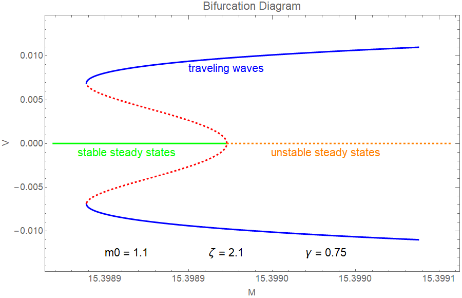
Figure 2: Bifurcation diagram, $m_{0}=1.1$, $\zeta=2.1$, $\gamma=0.75$.

Conjecture 5.3.

In the range of the parameters such that the total myosin mass $M$ of traveling wave solutions decreases in $V$ for small $V$, these solutions are nonlinearly unstable.

This Conjecture explains the nature of symmetry breaking at the onset of motion via instability of traveling for small velocities. Such a discontinuous transition from the rest to the steady motion has been observed in experiments and in direct numerical simulations of free boundary and phase field models [22],[25]. Note that the plots of the asymptotic solutions of the model (7)–(11) are obtained via rigorous analysis based on the Crandall-Rabinowitz bifurcation theorem and spectral analysis. In the one-dimensional model [19],[20] which is generalized in this work the supercritical pitchfork bifurcation to traveling waves is observed. This underscores the difference between the 2D model and its 1D prototype. Note that more sophisticated models in 1D also capture subcritical bifurcation [21].

6 Nonlinear stability of radially symmetric steady states

As shown in Section 3, the linearized operator around radially symmetric steady states always has zero eigenvalue and therefore linear stability analysis is inconclusive for the nonlinear stability problem. Although Lyapunov function is not known in this problem, we show that the invariant

$$\int_{\Omega(t)}m(x,y,t)dxdy$$ (72)

(total myosin mass) replaces Lyapunov function in the proof of nonlinear stability. This invariant corresponds to the eigenvector described in (ii) Remark 3.1 in the following sense. If the nonlinear problem has such invariant, then the corresponding linearized problem also has analogous invariant obtained by linearization of (72) in $\Omega(t)$ and $m(x,y,t)$. This linear invariant is the eigenvector of the adjoint linearized operator. Recall that the linearized operator has another eigenvector (see (i) in Remark 3.1) due to translational invariance of the problem. In the stability analysis below this eigenvector is taken into account by the appropriate choice of the moving frame.

Consider a radially symmetric steady state with $R=R_{0}$ from the family (13) and assume that $R_{0}$ is such that the following conditions hold

(i)

$$m_{0}:=-\gamma/R_{0}+p_{\rm eff}(\pi R^{2}_{0})\leq\lambda_{3},\quad\zeta>m_{0},$$ (73)

where $\lambda_{3}$ is the third eigenvalue of the operator $-\Delta$ in $B_{R_{0}}$ with the Neumann boundary condition on $\partial B_{R_{0}}$.

(ii) the hydrostatic pressure $p_{\rm eff}$ satisfies

$$p_{\rm eff}^{\prime}(\pi R^{2}_{0})<-\Bigl{(}\gamma/R_{0}+2m_{0}\Bigr{)}/(2\pi R^{2}_{0}),$$ (74)

(iii)

$$\phi_{1}^{\prime}(R_{0})<1,$$ (75)

where $\phi_{1}$ is the solution of (27) with $R=R_{0}$ (cf. Theorem 3.3(i)).

Theorem 6.1.

Let radially symmetric steady state (13) with $R=R_{0}$ satisfy conditions (73)-(75), then this steady state is stable in the following sense. For any $\varepsilon>0$ there exists $\delta(\varepsilon)>0$ such that if the initial data satisfies

$$\Omega(0)=\{0\leq r<R_{0}+\delta\rho(\varphi)\}\quad\text{with}\ \|\rho_{0}\|_{H^{4}(-\pi,\pi)}<1,$$ (76)

$$\|m(x,y,0)-m_{0}\|_{H^{2}(\Omega(0))}<\delta,$$ (77)

$\frac{\partial}{\partial\nu}m\bigl{|}_{t=0}\bigr{.}=0$ on $\partial\Omega(0)$, and $\int_{\Omega(0)}m(x,y,0)dxdy=m_{0}\pi R_{0}^{2}$, then the solution $\Omega(t)$, $m(x,y,t)$ exists for all $t>0$ and satisfies

$$\Omega(t)=\varepsilon(X_{c}(t),0)+\{0\leq r<R_{0}+\varepsilon\rho(\varphi,t)\}\quad\text{with}\ \|\rho(\,\cdot,\,t)\|_{H^{4}(-\pi.\pi)}<1,|X_{c}(t)|\leq C,$$ (78)

$$\|m(x,y,t)-m_{0}\|_{H^{2}(\Omega(t))}<\varepsilon,$$ (79)

where $\varepsilon(X_{c}(t),0)$ is shifted location of the linearized center of mass of $\partial\Omega(t)$ defined in (15). Moreover $\|m(x,y,t)-m_{0}\|_{H^{2}(\Omega(t))}\to 0$, $\|\rho(\,\cdot,\,t)\|_{H^{4}(-\pi.\pi)}\to 0$ as $t\to\infty$.

Proof.

One can show by using Hille-Yosida theorem that the operator $\mathcal{A}$ is a generator of the $C_{0}$-semigroup $e^{\mathcal{A}t}U$ in the space $(m,\rho)=:U\in L^{2}(B_{R_{0}})\times(H^{1}_{\rm per}(-\pi,\pi)\setminus\{\cos\varphi\})$. As in Theorem 3.3 introduce $\tilde{\phi}:=\phi+{R_{0}}\frac{p_{\rm eff}^{\prime}(\pi{R_{0}}^{2})}{\zeta}\int_{-\pi}^{\pi}\rho d\varphi$. The operator $\lambda I-\mathcal{A}$ is defined for $\lambda>0$ via the bilinear form on $H^{1}(B_{R_{0}})\times(H^{7/2}_{\rm per}(-\pi,\pi)\setminus\{\cos\varphi\})$

$$(f,g)=(\lambda I-\mathcal{A})(m,\rho)\ \Longleftrightarrow \int_{B_{R_{0}}}\nabla m\cdot\nabla\mu dxdy+(\lambda-m_{0})\int_{B_{R_{0}}}m\mu dxdy$$

$$+\int_{B_{R_{0}}}\nabla\tilde{\phi}\cdot\nabla\tilde{\psi}dxdy+\zeta\int_{B_{R_{0}}}\tilde{\phi}\tilde{\psi}dxdy+\frac{\lambda\gamma}{R_{0}\zeta}\int_{-\pi}^{\pi}(\rho^{\prime}\varrho^{\prime}-\tilde{\rho}\tilde{\varrho})d\varphi$$

$$+\zeta m_{0}\int_{B_{R_{0}}}\tilde{\phi}\mu dxdy-\int_{B_{R_{0}}}m\tilde{\psi}dxdy$$

$$=\int_{B_{R_{0}}}f\mu dxdy+\frac{\lambda\gamma}{R_{0}\zeta}\int_{-\pi}^{\pi}(g^{\prime}\tilde{\varrho}^{\prime}-g\tilde{\varrho})d\varphi,$$

$$\quad\forall\mu\in H^{1}(B_{R_{0}}),\ \varrho\in H^{7/2}_{\rm per}(-\pi,\pi)\setminus\{\cos\varphi\},$$

where $\tilde{\rho}=\rho+{R_{0}^{3}}\frac{p_{\rm eff}^{\prime}(\pi{R_{0}}^{2})}{\gamma}\int_{-\pi}^{\pi}\rho d\varphi$, $\tilde{\varrho}=\varrho+{R_{0}^{3}}\frac{p_{\rm eff}^{\prime}(\pi{R_{0}}^{2})}{\gamma}\int_{-\pi}^{\pi}\varrho d\varphi$, $\tilde{\phi}=\phi+{R_{0}}\frac{p_{\rm eff}^{\prime}(\pi{R_{0}}^{2})}{\zeta}\int_{-\pi}^{\pi}\rho d\varphi$ and $\phi$ solves (18)–(19), and $\tilde{\psi}=\psi+{R_{0}}\frac{p_{\rm eff}^{\prime}(\pi{R_{0}}^{2})}{\zeta}\int_{-\pi}^{\pi}\varrho d\varphi$, $\psi$ solving (18)–(19) with $\mu$ in place of $m$ and $\varrho$ in place of $\rho$.

In order to proceed with the proof of nonlinear stability in Theorem 6.1 we first show the regularity and exponential decay of the semigroup $e^{\mathcal{A}t}$ generated by linearized operator $\mathcal{A}$.

Lemma 6.2.

(regularity and decay properties of solutions of the linearized problem (17)–(20)) Under the conditions of Theorem 6.1, the semigroup $e^{\mathcal{A}t}$ (where $\mathcal{A}$ is defined in (21)) has the following properties:

• (decay property) For any initial data $U(0)=(m(x,y,0),\rho(\varphi,0))\in L^{2}(B_{R_{0}})\times(H^{1}_{\rm per}(-\pi,\pi)\setminus\{\cos\varphi\})$ the solution $U(t)=e^{\mathcal{A}t}U(0)$ of system (17)–(20) is represented as

  $$U(t)=cU_{1}/\Pi+\tilde{U}(t),$$ (80)

  where $c=\int_{B_{R_{0}}}m(\tilde{x},\tilde{y},0)d\tilde{x}d\tilde{y}+m_{0}\int_{-\pi}^{\pi}\rho(\tilde{\varphi},0){R_{0}}d\tilde{\varphi}$, $U_{1}=((\gamma/{R_{0}}+2\pi p_{\rm eff}^{\prime}(\pi{R_{0}}^{2}){R_{0}},1)$, is the eigenvector of the operator $\mathcal{A}$ corresponding to zero eigenvalue, see Remark 3.1, $\Pi=\pi{R_{0}}^{2}(\gamma/R_{0}+2\pi p_{\rm eff}^{\prime}(\pi{R_{0}}^{2}){R_{0}})+2\pi{R_{0}}m_{0}$, and

  $$\|\tilde{U}(t)\|_{L^{2}(B_{R_{0}})\times(H^{1}(-\pi,\pi))}\leq Ce^{-\theta t}\|U(0)\|_{L^{2}(B_{R_{0}})\times(H^{1}(-\pi,\pi))}$$ (81)

  with some constants $\theta>0$, $C$. Moreover, for $t>1$ estimate (81) improves to

  $$\|\tilde{U}(t)\|_{H^{2}(B_{R_{0}})\times(H^{4}(-\pi,\pi))}\leq C_{1}e^{-\theta t}\|U(0)\|_{L^{2}(B_{R_{0}})\times(H^{1}(-\pi,\pi))}.$$ (82)

• (regularization) If $U(0)\in H^{2}_{N}(B_{R_{0}})\times(H^{4}_{\rm per}(-\pi,\pi)\setminus\{\cos\varphi\})$ then representation (80) holds with $\tilde{U}\in L^{2}((0,+\infty);H^{2}_{N}(B_{R_{0}})\times(H^{11/2}_{\rm per}(-\pi,\pi)\setminus\{\cos\varphi\})$ and

  $$\int_{0}^{\infty}\|\tilde{U}(t)\|^{2}_{H^{2}(B_{R_{0}})\times H^{11/2}(-\pi,\pi)}dt+\int_{0}^{\infty}\|\frac{d}{dt}\tilde{U}(t)\|^{2}_{L^{2}(B_{R_{0}})\times H^{5/2}(-\pi,\pi)}dt\leq C\|\tilde{U}(0)\|^{2}_{H^{2}(B_{R_{0}})\times H^{4}(-\pi,\pi)}.$$

• For any $T>0$ and $F(t)\in L^{2}((0,T);L^{2}(B_{R_{0}})\times(H^{5/2}_{\rm per}(-\pi,\pi)\setminus\{\cos\varphi\}))$ the solution $U(t)=\int_{0}^{t}e^{A(t-\tau)}F(\tau)d\tau$ of the Cauchy problem $\frac{d}{dt}U(t)=\mathcal{A}U(t)+F(t)$, $U(0)=0$ belongs to

  $$L^{2}((0,T);H^{2}_{N}(B_{R_{0}})\times H^{11/2}(-\pi,\pi))\cap H^{1}((0,T);L^{2}(B_{R_{0}})\times H^{5/2}(-\pi,\pi))$$

  and satisfies

  $$\int_{0}^{T}\|U(t)\|^{2}_{H^{2}(B_{R_{0}})\times H^{11/2}(-\pi,\pi)}dt +\int_{0}^{T}\Bigl{\|}\frac{d}{dt}U(t)\Bigr{\|}^{2}_{L^{2}(B_{R_{0}})\times H^{5/2}(-\pi,\pi)}dt$$

  $$\leq C(1+T^{2})\int_{0}^{T}\|F(t)\|^{2}_{L^{2}(B_{R_{0}})\times H^{5/2}(-\pi,\pi)}dt,\quad\forall 0\leq\tau\leq T,$$

  where $C$ is independent of $T$.

Remark 6.3.

Statement (i) establishes exponential stability of the linearized problem (17)–(20) up to the constant eigenvector $U_{1}$. Here constant $c$ is the linearized total myosin mass. Indeed, if $m_{0}+\varepsilon m_{\varepsilon}$ is a perturbation of the steady state myosin density, then the total myosin mass expands as

$$\int_{\Omega_{\varepsilon}}(m_{0}+\varepsilon m_{\varepsilon}(x,y,0))dxdy$$

$$\hskip 40.0pt=\int_{B_{R}}m_{0}dxdy+\varepsilon\left(\int_{B_{R}}m_{\varepsilon}dxdy+\frac{1}{\varepsilon}\left(\int_{\Omega_{\varepsilon}\setminus B_{R}}-\int_{B_{R}\setminus\Omega_{\varepsilon}}\right)m_{0}dxdy\right)+O(\varepsilon^{2})$$

$$\hskip 40.0pt=\int_{B_{R}}m_{0}dxdy+\varepsilon\left(\mathop{\underbrace{\int_{B_{R}}m_{\varepsilon}dxdy+m_{0}R_{0}\int_{-\pi}^{\pi}\rho(\tilde{\varphi},0)d\tilde{\varphi}}}_{\mathrm{linearized}\,\mathrm{total}\,\mathrm{myosin}\,\mathrm{mass}}\right)+O(\varepsilon^{2}).$$

Constant $\Pi$ is chosen such that if one substitutes $U(t)\equiv U_{1}$ into (80), then (80) becomes a trivial equality $U_{1}=cU_{1}/\Pi$ with $c=c(U_{1})=\Pi$. Constants $c$ and $\Pi$ can also be written as a projection in terms of dot-products:

$$c=(U(0)\cdot\left[\begin{array}[]{c}1\\ m_{0}\end{array}\right])_{L^{2}(B_{R}\times\partial B_{R})}\quad\text{ and }\quad\Pi=(U_{1}\cdot\left[\begin{array}[]{c}1\\ m_{0}\end{array}\right])_{L^{2}(B_{R}\times\partial B_{R})}.$$ (83)

Representation (80) combined with the estimate (81) show that time-dependent part $\tilde{U}(t)$ of the solution $U(t)$ is exponentially decaying in time, that is (81) establishes contraction property of the corresponding semi-group for sufficiently large time.

Statement (ii) establishes stability and regularity in stronger norms provided that initial conditions are sufficiently smooth. To explain the powers in (ii), note that $m$ belongs at least in $H^{2}(B_{R})$ (so that LHS of (20) in $L^{2}(B_{R})$). Then from (18) it follows that $\nabla\phi\in H^{5/2}(\partial B_{R})$. Next, if one differentiates (19) in $\varphi$, then it follows that $\rho\in H^{3+5/2=11/2}(\partial B_{R})$.

Statement (iii) is about the linearized problem if inhomogeneity ${F}(t)$ is added. This result is needed to extend stability of linearized problem to the nonlinear one by representing original problem $U_{t}=\mathcal{L}(U)$ as $U_{t}=\mathcal{A}U+F(t)$ with nonlinearity $F(t)=\mathcal{L}(U)-\mathcal{A}U$.

Proof.

We employ Fourier analysis, representing $U=e^{\mathcal{A}t}U(0)$ as

$$U=\sum_{n=0}^{\infty}(\hat{m}_{n}(r,t),\hat{\rho}_{n}(t))\cos n\varphi,$$ (84)

then each pair $(\hat{m}_{n}(r,t),\hat{\rho}_{n}(t))\cos n\varphi$ satisfies system (17)–(20) with $\phi=\hat{\phi}_{n}(r,t)\cos n\varphi$ solving for $n\geq 1$ the equation $\Delta(\hat{\phi}_{n}\cos n\varphi)+\hat{m}_{n}\cos n\varphi=\zeta\hat{\phi}_{n}\cos n\varphi$ with the boundary condition $\hat{\phi}_{n}=\frac{\gamma}{R^{2}\zeta}(1-n^{2})\hat{\rho}_{n}(t)\cos n\varphi$ on $\partial B_{R}$. In the case $n=0$ it is convenient to seek $\phi$ in the form $\phi=\tilde{\phi}_{0}(r,t)-2\pi{R_{0}}\hat{\rho}_{0}(t)p_{\rm eff}^{\prime}(\pi{R_{0}}^{2})/\zeta$ then $\Delta\tilde{\phi}_{0}+\hat{m}_{0}=\zeta\tilde{\phi}_{0}$ in $B_{R}$ and

$$\tilde{\phi}_{0}(R_{0},t)=\Bigl{[}\frac{\gamma}{R^{2}\zeta}+2\pi{R_{0}}\hat{p}_{\rm eff}^{\prime}(\pi{R_{0}}^{2})/\zeta\Bigr{]}\hat{\rho}_{0}(t)$$ (85)

Let us prove first the exponential stabilization of the zero mode. To this end integrate the equations $\Delta\tilde{\phi}_{0}+\hat{m}_{0}=\zeta\tilde{\phi}_{0}$ and $\partial_{t}\hat{m}_{0}=\Delta\hat{m}_{0}-m_{0}\Delta\tilde{\phi}_{0}$ over $B_{R_{0}}$ to obtain

$$\frac{2}{R_{0}}\frac{d}{dt}\hat{\rho}_{0}+\langle\hat{m}_{0}\rangle=\zeta\langle\tilde{\phi}_{0}\rangle,\quad\frac{d}{dt}\langle\hat{m}_{0}\rangle+\frac{2m_{0}}{R_{0}}\frac{d}{dt}\hat{\rho}_{0}=0.$$ (86)

The second equation (linearized myosin mass preservation) implies that $\langle\hat{m}_{0}\rangle+\frac{2m_{0}}{R_{0}}\hat{\rho}_{0}=M_{0}$ is conserved in time, therefore the first equation in (86) rewrites with the help of (85) as

$$\frac{2}{R_{0}}\frac{d}{dt}\hat{\rho}_{0}=\left(\frac{2m_{0}}{R_{0}}+\frac{\gamma}{{R_{0}}^{2}}+2\pi{R_{0}}p_{\rm eff}^{\prime}(\pi{R_{0}}^{2})\right)\hat{\rho}_{0}+\zeta(\langle\tilde{\phi}_{0}\rangle-\tilde{\phi}(R_{0},t))-M_{0}.$$ (87)

Subtracting $cU_{1}/\Pi$ from the solution $U$ we reduce the study to the case $M_{0}=0$, see Remark 6.3, hence

$$\frac{2}{R_{0}}\frac{d}{dt}\hat{\rho}_{0}=-\theta_{2}\hat{\rho}_{0}+\zeta\langle\tilde{\phi}_{0}\rangle,$$ (88)

where $-\theta_{2}:=\frac{2m_{0}}{R_{0}}+\frac{\gamma}{{R_{0}}^{2}}+2\pi{R_{0}}p_{\rm eff}^{\prime}(\pi{R_{0}}^{2})<0$.

Next multiply the equation $\partial_{t}\hat{m}_{0}=\Delta\hat{m}_{0}-m_{0}\Delta\tilde{\phi}_{0}$ by $\tilde{m}=\hat{m}_{0}-\langle\hat{m}_{0}\rangle$ and integrate over $B_{R_{0}}$:

$$\frac{d}{2dt}\int_{B_{R_{0}}}\tilde{m}^{2}dxdy=-\int_{B_{R_{0}}}|\nabla\tilde{m}|^{2}dxdy+m_{0}\int_{B_{R_{0}}}\tilde{m}^{2}dxdy-\zeta m_{0}\int_{B_{R_{0}}}\tilde{\phi}_{0}\tilde{m}dxdy.$$ (89)

Then we multiply the equation $\Delta\tilde{\phi}_{0}+\hat{m}_{0}=\zeta\tilde{\phi}_{0}$ by $\tilde{\phi}_{0}-\langle\tilde{\phi}_{0}\rangle$ and integrate over $B_{R_{0}}$:

$$\int_{B_{R_{0}}}\tilde{\phi}_{0}\tilde{m}dxdy=\zeta\int_{B_{R_{0}}}(\tilde{\phi}_{0}-\langle\tilde{\phi}_{0}\rangle)^{2}dxdy+\int_{B_{R_{0}}}|\nabla(\tilde{\phi}_{0}-\langle\tilde{\phi}_{0}\rangle)|^{2}dxdy-2\pi R_{0}\frac{d\hat{\rho}_{0}}{dt}(\tilde{\phi}_{0}(R_{0},t)-\langle\tilde{\phi}_{0}\rangle).$$

We use this equality in (89) to get

$$\frac{d}{2dt}\int_{B_{R_{0}}}\tilde{m}^{2}dxdy= -\int_{B_{R_{0}}}|\nabla\tilde{m}|^{2}dxdy+m_{0}\int_{B_{R_{0}}}\tilde{m}^{2}dxdy-\zeta m_{0}\int_{B_{R_{0}}}|\nabla(\tilde{\phi}_{0}-\langle\tilde{\phi}_{0}\rangle)|^{2}dxdy$$ (90)

$$-\zeta^{2}m_{0}\int_{B_{R_{0}}}(\tilde{\phi}_{0}-\langle\tilde{\phi}_{0}\rangle)^{2}dxdy+2\pi\zeta m_{0}R_{0}\frac{d\hat{\rho}_{0}}{dt}(\tilde{\phi}_{0}(R_{0},t)-\langle\tilde{\phi}_{0}\rangle).$$

Then using (87) and the inequality $\int_{B_{R}}|\nabla(\tilde{\phi}_{0}-\langle\tilde{\phi}_{0}\rangle)|^{2}dxdy+\zeta\int_{B_{R}}(\tilde{\phi}_{0}-\langle\tilde{\phi}_{0}\rangle)^{2}dxdy\geq Q(\tilde{\phi}_{0}(R,t)-\langle\tilde{\phi}_{0}\rangle)^{2}$ (see (39)) we get

$$\frac{d}{2dt}\int_{B_{R_{0}}}\tilde{m}^{2}dxdy\leq -\int_{B_{R}}|\nabla\tilde{m}|^{2}dxdy+m_{0}\int_{B_{R_{0}}}\tilde{m}^{2}dxdy-\zeta m_{0}Q(\tilde{\phi}({R_{0}})-\langle\tilde{\phi}\rangle)^{2}$$ (91)

$$-4\pi m_{0}\left(\frac{d\hat{\rho}_{0}}{dt}\right)^{2}+\pi m_{0}R_{0}\left(\frac{2m_{0}}{R_{0}}+\frac{\gamma}{R^{2}}+2\pi Rp_{\rm eff}^{\prime}(\pi R^{2}_{0})\right)\frac{d}{dt}\hat{\rho}_{0}^{2}.$$

Since $m_{0}$ is less than the third eigenvalue of the Neumann Laplacian, by Proposition 6.5 we have $\int_{B_{R}}|\nabla\tilde{m}|^{2}dxdy-m_{0}\int_{B_{R}}\tilde{m}^{2}dxdy\geq\theta_{1}\int_{B_{R}}\tilde{m}^{2}dxdy$ for some $\theta_{1}>0$. Then using (87) once more we get

$$\frac{d}{2dt}\int_{B_{R_{0}}}\tilde{m}^{2}dxdy+(\pi m_{0}R_{0}+2Qm_{0}/(\zeta R_{0}))\theta_{2}\frac{d}{dt}\hat{\rho}_{0}^{2}\leq-\theta_{1}\int_{B_{R}}|\tilde{m}|^{2}dxdy-\theta_{3}\hat{\rho}_{0}^{2},$$ (92)

$\theta_{3}=Q\theta_{2}^{2}/\zeta^{2}>0$, this yields exponential decay of $\|\hat{m}_{0}\|_{L^{2}}$ and $|\hat{\rho}_{0}|$ as $t\to+\infty$.

Exponential decay of other modes is more simple to show (as in Theorem 3.3). For the component $n=1$ we have $\hat{\rho}_{1}=0$ for all $t\geq 0$, then using positive definiteness of the form (40) we get $\|\hat{m}_{1}\|_{L^{2}}^{2}\leq e^{-\theta_{4}t}\|\hat{m}_{1}\|^{2}|_{t=0}$, $\theta_{4}>0$. For higher harmonics, $n\geq 2$, we write $\partial_{t}\hat{m}_{n}\cos n\varphi=\Delta(\hat{m}_{n}\cos n\varphi)-m_{0}\Delta(\hat{\phi}_{n}\cos n\varphi)=\Delta(\hat{m}_{n}\cos n\varphi)+m_{0}\hat{m}_{n}\cos n\varphi-\zeta m_{0}\hat{\phi}_{n}\cos n\varphi$ multiply by $\hat{m}_{n}\cos n\varphi$ and integrate over $B_{R_{0}}$ to obtain, using the equality $\hat{m}_{n}\cos n\varphi=\zeta\hat{\phi}_{n}\cos n\varphi-\Delta(\hat{\phi}_{n}\cos n\varphi)$ and boundary conditions $\partial_{r}\hat{\phi}_{n}(R_{0})=\frac{d\hat{\rho}_{n}}{dt}$, $\hat{\phi}_{n}(R_{0})=-\frac{\gamma(n^{2}-1)}{R^{2}\zeta}\hat{\rho}_{n}$ ,

$$\frac{d}{4dt}\int_{B_{R_{0}}}\hat{m}^{2}_{n}dxdy= -\int_{B_{R_{0}}}|\nabla(\hat{m}_{n}\cos n\varphi)|^{2}dxdy+\frac{m_{0}}{2}\int_{B_{R_{0}}}\hat{m}^{2}_{n}dxdy$$ (93)

$$-\zeta m_{0}\int_{B_{R_{0}}}|\nabla(\hat{\phi}_{n}\cos n\varphi)|^{2}dxdy-\frac{\zeta^{2}m_{0}}{2}\int_{B_{R_{0}}}\hat{\phi}^{2}_{n}dxdy+\pi\frac{m_{0}\gamma(1-n^{2})}{2R_{0}}\frac{d}{dt}\hat{\rho}^{2}_{n}(t),$$

where $\rho(\varphi,t)=\hat{\rho}(t)\cos n\varphi$. Observe that for every function $\phi(r)$ one has

$$\int_{B_{R_{0}}}|\nabla(\phi(r)\cos n\varphi)|^{2}dxdy\geq|\phi(R_{0})|^{2}\int_{B_{R_{0}}}|\nabla\left((r/R_{0})^{n}\cos n\varphi\right)|^{2}dxdy=\pi n|\phi(R_{0})|^{2}.$$ (94)

Plugging this bound into (93) and applying Gronwall’s lemma we obtain

$$(\|\hat{m}_{n}(r,t)\|_{L^{2}(B_{R_{0}})}^{2}+n^{2}|\hat{\rho}_{n}(t)|^{2})\leq e^{-\overline{\theta}_{1}(n)t}(\|\hat{m}_{n}(r,0)\|_{L^{2}(B_{R_{0}})}^{2}+n^{2}|\hat{\rho}_{n}(0)|^{2})\quad\text{with}\ \overline{\theta}_{1}(n)\geq cn^{2},$$ (95)

where $c>0$. This proves (81). Also estimates (95) yield (82) via a bootstrap procedure described in the proof of (iii).

Now we proceed with item (iii). Represent $F(t)=(f(r,\varphi,t),g(\varphi,t))$ as $F(t)=s(t)U_{1}/\Pi+\tilde{F}$, where $s(t)=\int_{B_{R_{0}}}fdxdy+m_{0}R_{0}\int_{-\pi}^{\pi}gd\varphi$ and $\tilde{F}=(\tilde{f},\tilde{g})$ satisfies $\int_{B_{R_{0}}}\tilde{f}dxdy+m_{0}R_{0}\int_{-\pi}^{\pi}\tilde{g}d\varphi=0$ for all $t$. Then

$$U(t)=U_{1}\int_{0}^{t}s(\tau)d\tau/\Pi+\tilde{U},\quad\tilde{U}=(\tilde{m}(r,\varphi,t),\tilde{\rho}(\varphi,t))$$

and by item (i) we have

$$\|\tilde{U}(t)\|_{L^{2}(B_{R_{0}})\times H^{1}(-\pi,\pi)}\leq u(t):=C\int_{0}^{t}e^{-\theta(t-\tau)}\|F(\tau)\|_{L^{2}(B_{R_{0}})\times H^{1}(-\pi,\pi)}d\tau.$$

Since

$$\frac{du}{dt}u+\theta u^{2}=Cu(t)\|F(t)\|_{L^{2}(B_{R_{0}})\times H^{1}(-\pi,\pi)}\leq\frac{C^{2}}{2\theta}\|F(t)\|^{2}_{L^{2}(B_{R_{0}})\times H^{1}(-\pi,\pi)}+\frac{\theta}{2}u^{2},$$

it holds that

$$\int_{0}^{T}u^{2}dt\leq\frac{C^{2}}{\theta^{2}}\int_{0}^{T}\|F(t)\|^{2}_{L^{2}(B_{R_{0}})\times H^{1}(-\pi,\pi)}dt.$$

In particular, for every Fourier component $\tilde{\rho}_{n}(t)$ of $\tilde{\rho}=\sum\tilde{\rho}_{n}(t)\cos n\varphi$ we have

$$\int_{0}^{T}\tilde{\rho}_{n}^{2}(t)dt\leq C\int_{0}^{T}\|F(t)\|^{2}_{L^{2}(B_{R_{0}})\times H^{1}(-\pi,\pi)}dt.$$ (96)

To improve (96) for $n>2$ expand $f$, $g$, $\tilde{m}$ and $\tilde{\phi}$ into Fourier series $f=\sum f_{n}(r,t)\cos n\varphi$, $g=\sum g_{n}(t)\cos n\varphi$, $\tilde{m}=\sum\tilde{m}_{n}(r,t)\cos n\varphi$, $\tilde{\phi}=\sum\tilde{\phi}_{n}(r,t)\cos n\varphi$., where $\tilde{\phi}$ is the solution of problem (100). Then, arguing as in the derivation of (93) we get for $n>2$

$$\frac{d}{4dt}\int_{B_{R}}\tilde{m}^{2}_{n}dxdy= -\int_{B_{R}}|\nabla(\tilde{m}_{n}\cos n\varphi)|^{2}dxdy+\frac{m_{0}}{2}\int_{B_{R}}\tilde{m}^{2}_{n}dxdy+\frac{1}{2}\int_{B_{R}}f_{n}\tilde{m}_{n}dxdy$$ (97)

$$-\zeta m_{0}\int_{B_{R}}|\nabla(\tilde{\phi}_{n}\cos n\varphi)|^{2}dxdy-\frac{\zeta^{2}m_{0}}{2}\int_{B_{R}}\tilde{\phi}^{2}_{n}dxdy$$

$$+\pi\frac{m_{0}\gamma(1-n^{2})}{2R_{0}}\frac{d}{dt}\tilde{\rho}^{2}_{n}(t)-\pi\frac{m_{0}\gamma(1-n^{2})}{R_{0}}g_{n}(t)\tilde{\rho}_{n}(t),$$

Now we use here the bound (94), integrate the result from $0$ to $T$ in time to obtain that

$$cn^{5}\int_{0}^{T}\tilde{\rho}_{n}^{2}(t)dt\leq C\int_{0}^{T}\Bigl{(}\int_{B_{R_{0}}}f_{n}^{2}dxdy+n^{2}g_{n}^{2}(t)\Bigr{)}dt,\quad n>2,$$ (98)

where $c>0$ and $C$ are independent of $n$, $t$ and $T$. Thus (96) and (98) imply that $\|\rho\|_{L^{2}(0,T;H^{5/2}(-\pi,\pi))}\leq C\|F\|_{L^{2}(0,T;B_{R_{0}})\times H^{1}(-\pi,\pi))}$. Then, by elliptic estimates applied to $-\Delta\tilde{\phi}+\zeta\tilde{\phi}=\tilde{m}$ in $B_{R_{0}}$ with the boundary condition $\tilde{\phi}=\frac{\gamma}{R^{2}\zeta}(\tilde{\rho}^{\prime\prime}+\tilde{\rho})$ on $\partial B_{R}$ we have $\int_{0}^{T}\|\tilde{\phi}\|^{2}_{H^{2}(B_{R_{0}})}dt\leq C\int_{0}^{T}\|F(t)\|^{2}_{L^{2}(B_{R_{0}})\times H^{1}(-\pi,\pi)}dt$. This allows us to improve bound for $\tilde{m}$, applying parabolic estimates to the equation $\partial_{t}\tilde{m}-\Delta\tilde{m}+\tilde{m}=(m_{0}+1)\tilde{m}-\zeta m_{0}\tilde{\phi}$ (where we consider the right hand side as known) with the boundary condition $\partial_{r}\tilde{m}=0$ on $\partial B_{R_{0}}$. We find that

$$\int_{0}^{T}(\|\tilde{m}\|^{2}_{H^{2}(B_{R_{0}})}+\|\partial_{t}\tilde{m}\|^{2}_{L^{2}(B_{R_{0}})})dt \leq C\int_{0}^{T}\|(m_{0}+1)\tilde{m}-\zeta m_{0}\tilde{\phi}\|^{2}_{L^{2}(B_{R_{0}})}dt$$ (99)

$$\leq C\int_{0}^{T}\|F(t)\|^{2}_{L^{2}(B_{R_{0}})\times H^{1}(-\pi,\pi)}dt.$$

We also improve bounds (98) for $n>2$. To this end represent the solution $\tilde{\phi}$ of

$$\Delta\tilde{\phi}+\tilde{m}=\zeta\tilde{\phi}\quad\text{in}\ B_{R_{0}},\quad\tilde{\phi}=\frac{\gamma}{R^{2}_{0}\zeta}(\tilde{\rho}^{\prime\prime}+\tilde{\rho})\quad\text{on}\ \partial B_{R_{0}}$$ (100)

as $\tilde{\phi}=\tilde{\phi}^{(1)}+\tilde{\phi}^{(2)}$, where

$$\Delta\tilde{\phi}^{(1)}=\zeta\tilde{\phi}^{(1)}\quad\text{in}\ B_{R_{0}},\quad\tilde{\phi}^{(1)}=\frac{\gamma}{R^{2}\zeta}(\tilde{\rho}^{\prime\prime}+\tilde{\rho})\quad\text{on}\ \partial B_{R_{0}},$$

$$\Delta\tilde{\phi}^{(2)}+\tilde{m}=\zeta\tilde{\phi}^{(2)}\quad\text{in}\ B_{R_{0}},\quad\tilde{\phi}^{(2)}=0\quad\text{on}\ \partial B_{R_{0}}.$$

Next expand $\tilde{\phi}^{(1)}$ and $\tilde{\phi}^{(2)}$ into the Fourier series $\tilde{\phi}^{(1)}=\sum\tilde{\phi}_{n}^{(1)}(r,t)\cos n\varphi$, $\tilde{\phi}^{(2)}=\sum\tilde{\phi}_{n}^{(2)}(r,t)\cos n\varphi$ and multiply (100) by $\tilde{\phi}_{n}(r,t)\cos n\varphi$, $n\geq 2$, to find, integrating over $B_{R_{0}}$

$$\int_{B_{R_{0}}}(|\nabla(\tilde{\phi}_{n}\cos n\varphi)|^{2}+\frac{1}{2}(\zeta\tilde{\phi}_{n}^{2}-m\tilde{\phi}_{n}))dxdy =\int_{-\pi}^{\pi}\tilde{\phi}_{n}\partial_{r}\tilde{\phi}_{n}R_{0}\cos^{2}n\varphi d\varphi$$ (101)

$$=\frac{\pi\gamma}{R_{0}\zeta}(1-n^{2})\tilde{\rho}_{n}(t)\left(\frac{d\tilde{\rho}_{n}(t)}{dt}-g_{n}(t)\right).$$

On the other hand, the left hand side of (101) rewrites as

$$\int_{B_{R_{0}}}\left(|\nabla(\tilde{\phi}_{n}^{(1)}\cos n\varphi)|^{2}+\frac{\zeta}{2}(\tilde{\phi}_{n}^{(1)})^{2}\right)dxdy+\frac{\gamma\pi}{{R_{0}}\zeta}(1-n^{2})\tilde{\rho}_{n}(t)\partial_{r}\tilde{\phi}_{n}^{(2)}(R_{0},t),$$

and using (94) we obtain

$$cn^{5}\tilde{\rho}^{2}_{n}(t)+\frac{\pi\gamma}{2R_{0}\zeta}(n^{2}-1)\frac{d\tilde{\rho}_{n}^{2}(t)}{dt}\leq\frac{C}{n}\left(\bigl{(}\partial_{r}\tilde{\phi}_{n}^{(2)}(R_{0},t)\bigr{)}^{2}+g_{n}^{2}\right),$$ (102)

with $c>0$ and $C$ independent of $n$. Now multiply (102) by $n^{6}$ integrate in $t$ from $0$ to $T$ and add up the inequalities obtained to find that

$$\int_{0}^{T}\|\tilde{\rho}\|_{H^{11/2}(-\pi,\pi)}^{2}dt\leq C_{1}\int_{0}^{T}\|\partial_{r}\tilde{\phi}^{(2)}\|_{H^{5/2}(-\pi,\pi)}^{2}dt+C_{2}\int_{0}^{T}\|F(t)\|^{2}_{L^{2}(B_{R_{0}})\times H^{5/2}(-\pi,\pi)}dt.$$ (103)

It remains to note that by elliptic estimates that $\|\tilde{\phi}^{(2)}\|_{H^{4}(B_{R_{0}})}\leq C\|\tilde{m}\|_{H^{2}(B_{R_{0}})}$, which yields $\|\partial_{r}\tilde{\phi}^{(2)}\|_{H^{5/2}(-\pi,\pi)}\leq C\|\tilde{m}\|_{H^{2}(B_{R_{0}})}$, and exploit (99) to obtain the required bound for $\|\tilde{\rho}\|_{H^{11/2}(-\pi,\pi)}$ in $L^{2}(0,T)$. Also, since $\partial_{t}\tilde{\rho}=\partial_{r}\tilde{\phi}^{(1)}+\partial_{r}\tilde{\phi}_{2}$ and $\|\tilde{\phi}^{(1)}\|_{H^{4}(B_{R_{0}})}\leq C\|\tilde{\rho}\|_{H^{11/2}(-\pi,\pi)}$ we have $\int_{0}^{T}\|\partial_{t}\tilde{\rho}\|^{2}_{H^{5/2}(-\pi,\pi)}dt\leq C_{2}\int_{0}^{T}\|F(t)\|^{2}_{L^{2}(B_{R_{0}})\times H^{5/2}(-\pi,\pi)}dt$.

To prove (ii) we first obtain from (95) the following bound for the $\rho$-component $\tilde{\rho}$ of $\tilde{U}$,

$$\int_{0}^{\infty}\|\tilde{\rho}\|^{2}_{H^{3}(-\pi,\pi)}dt\leq C\|\tilde{U}(0)\|^{2}_{H^{1}(B_{R_{0}})\times H^{2}(-\pi,\pi)}.$$ (104)

By (i) we also know that $\|\tilde{m}\|_{L^{2}(B_{R_{0}})}\leq Ce^{-\theta t}\|U(0)\|_{L^{2}(B_{R_{0}})\times(H^{1}(-\pi,\pi))}$, therefore, arguing as in item (iii) one can show that

$$\int_{0}^{\infty}(\|\tilde{m}\|^{2}_{H^{2}(B_{R_{0}})}+\|\partial_{t}\tilde{m}\|^{2}_{L^{2}(B_{R_{0}})})dt\leq C\int_{0}^{\infty}\|(m_{0}+1)\tilde{m}-\zeta m_{0}\tilde{\phi}\|^{2}_{L^{2}(B_{R_{0}})}\leq C\|\tilde{U}(0)\|^{2}_{H^{1}(B_{R_{0}})\times H^{2}(-\pi,\pi)}.$$ (105)

Following further the lines of the proof of item (iii) we eventually get

$$\int_{0}^{\infty}\|\tilde{\rho}\|_{H^{11/2}(-\pi,\pi)}^{2}dt\leq C_{1}\int_{0}^{\infty}\|\partial_{r}\tilde{\phi}^{(2)}\|_{H^{5/2}(-\pi,\pi)}^{2}dt+C_{2}\|\rho\|^{2}_{H^{4}(-\pi,\pi)}\bigl{|}_{t=0}.$$ (106)

Then again arguing as in item (iii) we complete the proof of the Lemma. ∎

Corollary 6.4.

Under conditions of Theorem 6.1 the following uniform in $t\in[0,T]$ bounds hold

$$\|e^{\mathcal{A}t}U_{0}\|_{H^{1}(B_{R_{0}})\times H^{4}(-\pi,\pi)}\leq C\|U_{0}\|_{H^{2}(B_{R_{0}})\times H^{4}(-\pi,\pi)}\quad\forall U_{0}\in H^{2}_{N}(B_{R_{0}})\times H^{4}(-\pi,\pi),$$

$$\|U(t)\|_{H^{1}(B_{R_{0}})\times H^{4}(-\pi,\pi)}\leq CT\int_{0}^{T}\|F(t)\|^{2}_{L^{2}(B_{R_{0}})\times H^{5/2}(-\pi,\pi)}dt,\quad\forall F\in L^{2}(0,T;L^{2}(B_{R_{0}})\times H^{5/2}(-\pi,\pi)),$$

where $U(t)=\int_{0}^{t}e^{A(t-\tau)}F(\tau)d\tau$, $C$ is independent of $T$.

Proof.

To get the sought bound for the $\rho$-component, we write

$$\|\rho(t)\|^{2}_{H^{4}(-\pi,\pi)}= C\|\rho(0)\|^{2}_{H^{4}(-\pi,\pi)}+C\int_{0}^{t}\int_{-\pi}^{\pi}(\partial^{4}_{\varphi^{4}}\rho\partial_{t}\partial^{4}_{\varphi^{4}}\rho+\rho\partial_{t}\rho)d\varphi dt$$

$$\leq C\|\rho(0)\|^{2}_{H^{4}(-\pi,\pi)}+C\int_{0}^{t}\|\partial_{t}\rho\|_{H^{5/2}(-\pi,\pi)}\|\rho\|_{H^{11/2}(-\pi,\pi)}dt$$

and then use bounds from Lemma 6.2. The $m$-component is treated similarly. ∎

Although the function $\phi$ appearing in the linearized problem (17)–(20) does not belong to the phase space, it is convenient to introduce the operator $S_{\phi}(m,\rho)$ which assigns to the given $m$ and $\rho$ the unique solution $S_{\phi}(m,\rho)$of the problem

$$\Delta S_{\phi}+m=\zeta S_{\phi}+p_{\rm eff}^{\prime}(\pi R^{2})R\int_{-\pi}^{\pi}\rho(\varphi)d\varphi\quad\text{in}\ B_{R},\quad S_{\phi}=\frac{\gamma}{R^{2}\zeta}(\rho^{\prime\prime}+\rho)\quad\text{on}\ \partial B_{R}.$$ (107)

To deal with shift invariance we rewrite problem (7)–(11) in moving frame with center at $\varepsilon(X_{c,\varepsilon}(t),0)$, then $\Omega_{\varepsilon}(t)=\tilde{\Omega}_{\varepsilon}(t)+\varepsilon(X_{c,\varepsilon}(t),0)$ and (9) after introducing the polar coordinates $(\tilde{r},\tilde{\varphi})$ to parameterize $\tilde{\Omega}_{\varepsilon}(t)$, $\tilde{\Omega}_{\varepsilon}(t)=\{0\leq\tilde{r}<R_{0}+\varepsilon\rho_{\varepsilon}(\tilde{\varphi},t)\}$, reads

$$\partial_{t}\rho_{\varepsilon}+\dot{X}_{c,\varepsilon}\left(\cos\varphi+\frac{\varepsilon\rho^{\prime}_{\varepsilon}\sin\varphi}{R_{0}+\varepsilon\rho_{\varepsilon}}\right)=\frac{\sqrt{\varepsilon^{2}(\rho^{\prime}_{\varepsilon})^{2}+(R_{0}+\varepsilon\rho_{\varepsilon})^{2}}}{\varepsilon(R_{0}+\varepsilon\rho_{\varepsilon})}\partial_{\nu}\phi\quad\text{on}\ \partial\tilde{\Omega}_{\varepsilon}(t),$$ (108)

while (10) becomes

$$\partial_{t}m=\Delta m+\varepsilon\dot{X}_{c,\varepsilon}\partial_{x}m-{\rm div}(m\nabla\phi),\quad\text{in}\ \tilde{\Omega}_{\varepsilon}(t).$$ (109)

We impose the orthogonality condition $\int_{-\pi}^{\pi}\partial_{t}\rho_{\varepsilon}\cos\varphi d\varphi=0$ which yields the following equation governing the evolution of $X_{c,\varepsilon}$

$$\dot{X}_{c,\varepsilon}\left(1+\frac{\varepsilon}{2\pi}\int_{-\pi}^{\pi}\frac{\rho^{\prime}_{\varepsilon}\sin 2\varphi}{R_{0}+\varepsilon\rho_{\varepsilon}}d\varphi\right)=\frac{1}{\pi}\int_{-\pi}^{\pi}\frac{\sqrt{\varepsilon^{2}(\rho^{\prime}_{\varepsilon})^{2}+(R_{0}+\varepsilon\rho_{\varepsilon})^{2}}}{\varepsilon(R_{0}+\varepsilon\rho_{\varepsilon})}\partial_{\nu}\phi\cos\varphi d\varphi.$$ (110)

Next we introduce a transformation to reduce the study of the free boundary problem to a problem in the fixed disk. We introduce local coordinates in an inner neighborhood of $\partial\tilde{\Omega}_{\varepsilon}$ by setting $\tilde{\Omega}_{\varepsilon}\ni(\tilde{x},\tilde{y})\mapsto(r,\varphi)\in(2R_{0}/3,R_{0})\times(-\pi,\pi)$,

$$\tilde{x}=(R_{0}+\varepsilon\rho_{\varepsilon}(\varphi,t))\cos\varphi+(r-R_{0})\frac{\varepsilon\rho^{\prime}\sin\varphi+(R_{0}+\varepsilon\rho_{\varepsilon})\cos\varphi}{\sqrt{\varepsilon^{2}(\rho^{\prime}_{\varepsilon})^{2}+(R_{0}+\varepsilon\rho_{\varepsilon})^{2}}},$$ (111)

$$\tilde{y}=(R_{0}+\varepsilon\rho_{\varepsilon}(\varphi,t))\sin\varphi+(r-R_{0})\frac{-\varepsilon\rho^{\prime}_{\varepsilon}\cos\varphi+(R_{0}+\varepsilon\rho_{\varepsilon})\sin\varphi}{\sqrt{\varepsilon^{2}(\rho^{\prime}_{\varepsilon})^{2}+(R_{0}+\varepsilon\rho_{\varepsilon})^{2}}}$$

Note that the normal vector on the boundary is given by

$$\nu_{x}=\frac{\varepsilon\rho^{\prime}_{\varepsilon}\sin\varphi+(R_{0}+\varepsilon\rho_{\varepsilon})\cos\varphi}{\sqrt{\varepsilon^{2}(\rho^{\prime}_{\varepsilon})^{2}+(R_{0}+\varepsilon\rho_{\varepsilon})^{2}}},\quad\nu_{y}=\frac{-\varepsilon\rho^{\prime}_{\varepsilon}\cos\varphi+(R_{)}+\varepsilon\rho_{\varepsilon})\sin\varphi}{\sqrt{\varepsilon^{2}(\rho^{\prime}_{\varepsilon})^{2}+(R_{)}+\varepsilon\rho_{\varepsilon})^{2}}}.$$

Also observe that $R_{0}-r$ in (111) represents the distance from the boundary $\partial\tilde{\Omega}_{\varepsilon}$ to $(\tilde{x},\tilde{y})$ and therefore the normal derivative on the boundary $\partial\tilde{\Omega}_{\varepsilon}(t)$ becomes the derivative in $r$ on $\partial B_{R_{0}}$ even though the domain $\tilde{\Omega}_{\varepsilon}$ is obtained by non-radial perturbations of the disk $B_{R}$:

$$\partial_{\nu}m(\tilde{x}(R_{0},\varphi),\tilde{y}(R_{0},\varphi))=\partial_{r}m(\tilde{x}(r,\varphi),\tilde{y}(r,\varphi))\Bigl{|}_{r=R_{0}}\Bigr{.}$$

In order to avoid singular behavior at the origin, the coordinate transformation (111) is defined in a neighborhood of the boundary $\partial\tilde{\Omega}_{\varepsilon}$. Then the extension from this neighborhood to the entire domain $\tilde{\Omega}_{\varepsilon}$ by $(r,\varphi)\in[0,R_{0})\times[-\pi,\pi)$ is done by employing a cutoff function $\chi\in C^{\infty}$, $\chi(r)=1$ for $r>2R_{0}/3$ and $\chi(r)=0$ for $r<R_{0}/2$:

$$\tilde{x}=\Bigl{[}(R_{0}+\varepsilon\rho_{\varepsilon}(\varphi,t))\cos\varphi+(r-R_{0})\frac{\varepsilon\rho^{\prime}_{\varepsilon}\sin\varphi+(R_{0}+\varepsilon\rho_{\varepsilon})\cos\varphi}{\sqrt{\varepsilon^{2}(\rho^{\prime}_{\varepsilon})^{2}+(R_{0}+\varepsilon\rho_{\varepsilon})^{2}}}\Bigr{]}\chi(r)+(1-\chi(r))r\cos\varphi,$$

$$\tilde{y}=\Bigl{[}(R_{0}+\varepsilon\rho_{\varepsilon}(\varphi,t))\sin\varphi+(r-R_{0})\frac{-\varepsilon\rho^{\prime}_{\varepsilon}\cos\varphi+(R_{0}+\varepsilon\rho_{\varepsilon})\sin\varphi}{\sqrt{\varepsilon^{2}(\rho^{\prime}_{\varepsilon})^{2}+(R_{0}+\varepsilon\rho_{\varepsilon})^{2}}}\Bigr{]}\chi(r)+(1-\chi(r))r\sin\varphi,$$

or

$$\tilde{x}=(r+\varepsilon\eta)\cos\varphi-\varepsilon\sigma\sin\varphi,\quad\tilde{y}=(r+\varepsilon\eta)\sin\varphi+\varepsilon\sigma\cos\varphi,$$ (112)

where

$$\eta(r,\rho_{\varepsilon},\rho^{\prime}_{\varepsilon})=\frac{\varepsilon(\rho_{\varepsilon}^{\prime})^{2}(R_{0}-r)}{\Bigl{(}R_{0}+\varepsilon\rho_{\varepsilon}+{\sqrt{\varepsilon^{2}(\rho^{\prime}_{\varepsilon})^{2}+(R_{0}+\varepsilon\rho_{\varepsilon})^{2}}}\Bigr{)}{\sqrt{\varepsilon^{2}(\rho^{\prime}_{\varepsilon})^{2}+(R_{0}+\varepsilon\rho_{\varepsilon})^{2}}}}\chi(r)+\rho_{\varepsilon}\chi(r),$$

$$\sigma(r,\rho_{\varepsilon},\rho^{\prime}_{\varepsilon})=(R_{0}-r)\frac{\rho^{\prime}_{\varepsilon}}{\sqrt{\varepsilon^{2}(\rho^{\prime}_{\varepsilon})^{2}+(R_{0}+\varepsilon\rho_{\varepsilon})^{2}}}\chi(r).$$

Represent $m$ and $\phi$ in the form

$$m(\tilde{x}(r,\varphi,t)+\varepsilon X_{c,\varepsilon}(t),\tilde{y}(r,\varphi,t),t) =m_{0}+\varepsilon m_{\varepsilon}(r,\varphi,t),$$

$$\quad\phi(\tilde{x}(r,\varphi,t)+\varepsilon X_{c,\varepsilon}(t),\tilde{y}(r,\varphi,t),t) =\phi_{0}+\varepsilon\phi_{\varepsilon}(r,\varphi,t)+\varepsilon p_{\rm eff}^{\prime}(\pi R^{2}_{0})\frac{R_{0}}{\zeta}\int_{-\pi}^{\pi}\rho_{\varepsilon}(\tilde{\varphi},t)d\tilde{\varphi},$$

then (7)–(11) rewrites as a problem whose linear part is the same as in (17)–(20), but with additional nonlinear terms $f_{1}$, $f_{2}$, $g_{1}$, and $g_{2}$:

$$\Delta\phi_{\varepsilon}+m_{\varepsilon}=\zeta\phi_{\varepsilon}+p_{\rm eff}^{\prime}(\pi R^{2}_{0})R_{0}\int_{-\pi}^{\pi}\rho_{\varepsilon}(\tilde{\varphi})d\tilde{\varphi}-\varepsilon f_{1}\quad\text{in}\ B_{R},$$ (113)

$$\phi_{\varepsilon}=\frac{\gamma}{R^{2}\zeta}(\rho^{\prime\prime}+\rho)+\varepsilon g_{1}\quad\text{on}\ \partial B_{R},$$ (114)

$$\partial_{t}\rho_{\varepsilon}=\partial_{r}\phi_{\varepsilon}-\frac{\cos\varphi}{\pi}\int_{-\pi}^{\pi}\partial_{r}\phi_{\varepsilon}\cos\tilde{\varphi}d\tilde{\varphi}+\varepsilon g_{2}\quad\text{on}\ \partial B_{R},$$ (115)

$$\partial_{t}m_{\varepsilon}=\Delta m_{\varepsilon}-m_{0}\Delta\phi_{\varepsilon}+\varepsilon f_{2}\quad\text{in}\ B_{R},$$ (116)

$$\partial_{r}m_{\varepsilon}=0\quad\text{on}\ \partial B_{R},$$ (117)

together with

$$\dot{X}_{c,\varepsilon}=\tilde{V},\quad\tilde{V}[\phi_{\varepsilon},\rho_{\varepsilon}]=\frac{1}{\pi\left(1+\frac{\varepsilon}{2\pi}\int_{-\pi}^{\pi}\frac{\rho^{\prime}_{\varepsilon}\sin 2\varphi}{R_{0}+\varepsilon\rho_{\varepsilon}}d\varphi\right)}\int_{-\pi}^{\pi}\frac{\sqrt{\varepsilon^{2}(\rho^{\prime}_{\varepsilon})^{2}+(R_{0}+\varepsilon\rho_{\varepsilon})^{2}}}{R_{0}+\varepsilon\rho_{\varepsilon}}\partial_{r}\phi_{\varepsilon}\cos\varphi d\varphi.$$ (118)

The additional term $f_{1}$ in (113) appears when applying the coordinate change (112) to (7) and linearizing $p_{\rm eff}(|\tilde{\Omega}_{\varepsilon}|)$,

$$f_{1}[\tilde{\phi}_{\varepsilon},\rho_{\varepsilon}]=\frac{1}{\varepsilon}p_{\rm eff}^{\prime}(\pi R^{2}_{0})R_{0}\int_{-\pi}^{\pi}\rho_{\varepsilon}(\tilde{\varphi},t)d\tilde{\varphi}-\frac{1}{\varepsilon^{2}}\left(p_{\rm eff}\Bigl{[}\int_{-\pi}^{\pi}(R_{0}+\varepsilon\rho_{\varepsilon}(\tilde{\varphi},t))^{2}\frac{d\tilde{\varphi}}{2}\Bigr{]}-p_{\rm eff}(\pi R_{0}^{2})\right)+L(\phi_{\varepsilon},\rho_{\varepsilon}),$$

where

$$L(\phi_{\varepsilon},\rho_{\varepsilon})= 2(a_{x}\cos\varphi+a_{y}\cos\varphi)\partial^{2}_{rr}\phi_{\varepsilon}+\varepsilon(a_{x}^{2}+a_{y}^{2})\partial^{2}_{rr}\phi_{\varepsilon}$$

$$+(\cos\varphi\partial_{r}a_{x}-b_{x}\sin\varphi+\frac{1}{r}(\cos\varphi\partial_{\varphi}a_{y}-\sin\varphi\partial_{\varphi}a_{x})+\sin\varphi\partial_{r}a_{y}+b_{y}\cos\varphi)\partial_{r}\phi_{\varepsilon}$$

$$+\varepsilon(a_{x}\partial_{r}a_{x}+b_{x}\partial_{\varphi}a_{x}+a_{y}\partial_{r}a_{y}+b_{y}\partial_{\varphi}a_{y})\partial_{r}\phi_{\varepsilon}$$

$$+2(b_{x}\cos\varphi-a_{x}\frac{\sin\varphi}{r}+a_{y}\frac{\cos\varphi}{r}+b_{y}\sin\varphi)\partial_{r\varphi}\phi_{\varepsilon}+2\varepsilon(a_{x}b_{x}+a_{y}b_{y})\partial_{r\varphi}\phi_{\varepsilon}$$

$$+(a_{x}\frac{\sin\varphi}{r^{2}}+\cos\varphi\partial_{r}b_{x}-b_{x}\frac{\cos\varphi}{r}-\frac{\sin\varphi}{r}\partial_{\varphi}b_{x}-a_{y}\frac{\cos\varphi}{r^{2}}+\sin\varphi\partial_{r}b_{y}-b_{y}\frac{\sin\varphi}{r}+\frac{\cos\varphi}{r}\partial_{\varphi}b_{y})\partial_{\varphi}\phi_{\varepsilon}$$

$$+\varepsilon(a_{x}\partial_{r}b_{x}+b_{x}\partial_{\varphi}b_{x}+a_{y}\partial_{r}b_{y}+b_{y}\partial_{\varphi}b_{y})\partial_{\varphi}\phi_{\varepsilon}$$

$$+2(b_{y}\frac{\cos\varphi}{r}-b_{x}\frac{\sin\varphi}{r})\partial^{2}_{\varphi\varphi}m_{\varepsilon}+\varepsilon(b_{x}^{2}+b_{y}^{2})\partial^{2}_{\varphi\varphi}\phi_{\varepsilon},$$

with

$$a_{x} =(\cos\varphi(\eta+\partial_{\varphi}\sigma)+\sin\varphi(\partial_{\varphi}\eta-\sigma))(\frac{1}{r}-\varepsilon Z)-rZ\cos\varphi,$$

$$a_{y} =(\cos\varphi(\sigma-\partial_{\varphi}\eta)+\sin\varphi(\eta+\partial_{\varphi}\sigma))(\frac{1}{r}-\varepsilon Z)-rZ\sin\varphi,$$

$$b_{x} =(\varepsilon Z-\frac{1}{r})(\sin\varphi\partial_{r}\eta+\cos\varphi\partial_{r}\sigma)+Z\sin\varphi,\ b_{y}=(\frac{1}{r}-\varepsilon Z)(\cos\varphi\partial_{r}\eta-\sin\varphi\partial_{r}\sigma)-Z\sin\varphi,$$

$$Z=\frac{\eta+\partial_{r}\eta+(1+\varepsilon\partial_{r}\eta)\partial_{\varphi}\sigma+\varepsilon\partial_{r}\sigma(\sigma-\partial_{\varphi}\eta)}{r(r+\varepsilon(\eta+\partial_{r}\eta+(1+\varepsilon\partial_{r}\eta)\partial_{\varphi}\sigma)+\varepsilon^{2}\partial_{r}\sigma(\sigma-\partial_{\varphi}\eta))}.$$

The term $f_{2}$ in (116) appears when applying change of variables (112) to (10),

$$f_{2}[m_{\varepsilon},\phi_{\varepsilon},\rho_{\varepsilon}]= L(m_{\varepsilon},\rho_{\varepsilon})-(m_{0}+\varepsilon m_{\varepsilon})L(\phi_{\varepsilon},\rho_{\varepsilon})-m_{\varepsilon}\Delta\phi_{\varepsilon}$$

$$+(\tilde{V}[\phi_{\varepsilon},\rho_{\varepsilon}]+\cos\varphi\partial_{t}\eta-\sin\varphi\partial_{t}\sigma)((\cos\varphi+\varepsilon a_{x})\partial_{r}m_{\varepsilon}+(\varepsilon b_{x}-\frac{\sin\varphi}{r})\partial_{\varphi}m_{\varepsilon})$$

$$+(\sin\varphi\partial_{t}\eta+\cos\varphi\partial_{t}\sigma)((\sin\varphi+\varepsilon a_{y})\partial_{r}m_{\varepsilon}+(\varepsilon b_{y}+\frac{\cos\varphi}{r})\partial_{\varphi}m_{\varepsilon})$$

$$-\left((\cos\varphi+\varepsilon a_{x})\partial_{r}m_{\varepsilon}+(\varepsilon b_{x}-\frac{\sin\varphi}{r})\partial_{\varphi}m_{\varepsilon}\right)\left((\cos\varphi+\varepsilon a_{x})\partial_{r}\tilde{\phi}_{\varepsilon}+(\varepsilon b_{x}-\frac{\sin\varphi}{r})\partial_{\varphi}\phi_{\varepsilon}\right)$$

$$-\left((\sin\varphi+\varepsilon a_{y})\partial_{r}m_{\varepsilon}+(\varepsilon b_{y}+\frac{\cos\varphi}{r})\partial_{\varphi}m_{\varepsilon}\right)\left((\sin\varphi+\varepsilon a_{y})\partial_{r}\tilde{\phi}_{\varepsilon}+(\varepsilon b_{y}+\frac{\cos\varphi}{r})\partial_{\varphi}\phi_{\varepsilon}\right).$$

Also,

$$g_{1}[\rho_{\varepsilon}]=-\frac{2\gamma(\rho_{\varepsilon}^{\prime})^{2}}{\zeta{((R_{0}+\varepsilon\rho_{\varepsilon})^{2}+\varepsilon^{2}(\rho^{\prime}_{\varepsilon})^{2})^{3/2}}}-\frac{\gamma((\rho_{\varepsilon}^{\prime\prime}+\rho_{\varepsilon})(2\rho_{\varepsilon}R_{0}+\varepsilon\rho_{\varepsilon}^{2})-R_{0}\rho_{\varepsilon}^{2})(R_{0}+\varepsilon\rho_{\varepsilon})}{\zeta R_{0}^{2}{((R_{0}+\varepsilon\rho_{\varepsilon})^{2}+\varepsilon^{2}(\rho^{\prime}_{\varepsilon})^{2})^{3/2}}}$$ (119)

$$+\frac{\gamma(R_{0}-\varepsilon\rho_{\varepsilon}^{\prime\prime}-\varepsilon\rho_{\varepsilon})(\rho^{\prime}_{\varepsilon})^{2}(2(R_{0}+\varepsilon\rho_{\varepsilon})^{2}+(\varepsilon\rho_{\varepsilon}^{\prime})^{2}+(R_{0}+\varepsilon\rho_{\varepsilon})\sqrt{(R_{0}+\varepsilon\rho_{\varepsilon})^{2}+(\varepsilon\rho^{\prime}_{\varepsilon})^{2}})}{\zeta R_{0}^{2}(R_{0}+\varepsilon\rho_{\varepsilon}+\sqrt{(R_{0}+\varepsilon\rho_{\varepsilon})^{2}+(\varepsilon\rho^{\prime}_{\varepsilon})^{2}}){((R_{0}+\varepsilon\rho_{\varepsilon})^{2}+\varepsilon^{2}(\rho^{\prime}_{\varepsilon})^{2})^{3/2}}}$$

$$g_{2}[\phi_{\varepsilon},\rho_{\varepsilon}]= \frac{\varepsilon(\rho_{\varepsilon}^{\prime})^{2}}{\Bigl{(}R_{0}+\varepsilon\rho_{\varepsilon}+{\sqrt{\varepsilon^{2}(\rho^{\prime}_{\varepsilon})^{2}+(R_{0}+\varepsilon\rho_{\varepsilon})^{2}}}\Bigr{)}{(R_{0}+\varepsilon\rho_{\varepsilon})}}\partial_{r}\phi_{\varepsilon}$$ (120)

$$+\frac{\int_{-\pi}^{\pi}\partial_{r}\phi_{\varepsilon}\cos\tilde{\varphi}d\tilde{\varphi}}{\pi\left(1+\frac{\varepsilon}{2\pi}\int_{-\pi}^{\pi}\frac{\rho^{\prime}_{\varepsilon}\sin 2\tilde{\varphi}}{R_{0}+\varepsilon\rho_{\varepsilon}}d\tilde{\varphi}\right)}\left[\frac{\cos\varphi}{2\pi}\int_{-\pi}^{\pi}\frac{\rho^{\prime}_{\varepsilon}\sin 2\tilde{\varphi}}{R_{0}+\varepsilon\rho_{\varepsilon}}d\tilde{\varphi}-\frac{\rho^{\prime}_{\varepsilon}\sin\varphi}{R_{0}+\varepsilon\rho_{\varepsilon}}\right]$$

$$-\varepsilon\frac{\cos\varphi+\frac{\rho^{\prime}_{\varepsilon}\sin\varphi}{R_{0}+\varepsilon\rho_{\varepsilon}}}{\pi\left(1+\frac{\varepsilon}{2\pi}\int_{-\pi}^{\pi}\frac{\rho^{\prime}_{\varepsilon}\sin 2\tilde{\varphi}}{R_{0}+\varepsilon\rho_{\varepsilon}}d\tilde{\varphi}\right)}\int_{-\pi}^{\pi}\frac{(\rho_{\varepsilon}^{\prime})^{2}\partial_{r}\phi_{\varepsilon}\cos\tilde{\varphi}d\tilde{\varphi}}{\Bigl{(}R_{0}+\varepsilon\rho_{\varepsilon}+{\sqrt{\varepsilon^{2}(\rho^{\prime}_{\varepsilon})^{2}+(R_{0}+\varepsilon\rho_{\varepsilon})^{2}}}\Bigr{)}{(R_{0}+\varepsilon\rho_{\varepsilon})}}.$$

The nonlinear terms $f_{1}$, $f_{2}$, $g_{1}$, $g_{2}$ in system (113)–(118) contain higher order derivatives, that is why regularity result (iii) in Lemma 6.2 is crucial for the solvability of this system.

The solvability of (113)–(118) is shown iteratively via the contraction mapping theorem. Namely in the initial step we solve (113)–(117) with given initial data and $f_{1}=f_{2}=0$, $g_{1}=g_{2}=0$ to obtain the first iteration $(m_{\varepsilon,0},\rho_{\varepsilon,0})=e^{\mathcal{A}t}(m_{\varepsilon}(r,\varphi,0),\rho_{\varepsilon}(\varphi,0))$, $\phi_{\varepsilon,0}=S_{\phi}(m_{\varepsilon,0},\rho_{\varepsilon,0})$. Without loss of generality we can assume that the function $\rho_{\varepsilon}(\varphi,0)$, which determines the initial shape, is orthogonal to $\cos\varphi$, for otherwise one modifies appropriately the initial position of the center $X_{c,\varepsilon}(0)$ of the reference steady state. Then semigroup $e^{\mathcal{A}t}$ is well defined for such initial data.

Next introduce new unknowns $\mu_{\varepsilon}:=m_{\varepsilon}-m_{\varepsilon,0}$, $\varrho_{\varepsilon}:=\rho_{\varepsilon}-\rho_{\varepsilon,0}$ and represent $\phi_{\varepsilon}$ as $\phi_{\varepsilon}=\psi_{\varepsilon}+\phi_{\varepsilon,0}+\varepsilon\overline{\psi}_{\varepsilon}$, where $\overline{\psi}_{\varepsilon}=\overline{\psi}_{\varepsilon}[\psi_{\varepsilon},\varrho_{\varepsilon},\psi_{\varepsilon,0},\rho_{\varepsilon,0}]$ solves

$$\Delta\overline{\psi}_{\varepsilon}=\zeta\overline{\psi}_{\varepsilon}-f_{1}[\psi_{\varepsilon}+\phi_{\varepsilon,0}+\varepsilon\overline{\psi}_{\varepsilon},\varrho_{\varepsilon}+\rho_{\varepsilon,0}]\ \quad\text{in}\ B_{R},$$ (121)

$$\overline{\psi}_{\varepsilon}=g_{1}[\varrho_{\varepsilon}+\rho_{\varepsilon,0}]\quad\text{on}\ \partial B_{R},$$ (122)

to rewrite equations (113)–(117) in the form

$$\Delta\psi_{\varepsilon}+\mu_{\varepsilon}=\zeta\psi_{\varepsilon}+p_{\rm eff}^{\prime}(\pi R^{2}_{0})R_{0}\int_{-\pi}^{\pi}\varrho_{\varepsilon}(\tilde{\varphi})d\tilde{\varphi}\quad\text{in}\ B_{R},$$ (123)

$$\psi_{\varepsilon}=\frac{\gamma}{R^{2}\zeta}(\varrho^{\prime\prime}_{\varepsilon}+\varrho_{\varepsilon})\quad\text{on}\ \partial B_{R},$$ (124)

$$\begin{aligned} \partial_{t}\varrho_{\varepsilon}=\partial_{r}\psi_{\varepsilon}-\frac{\cos\varphi}{\pi}\int_{-\pi}^{\pi}\partial_{r}\psi_{\varepsilon}\cos\tilde{\varphi}d\tilde{\varphi}+\varepsilon\Bigl{(}\partial_{r}\overline{\psi}_{\varepsilon}&-\frac{\cos\varphi}{\pi}\int_{-\pi}^{\pi}\partial_{r}\overline{\psi}_{\varepsilon}\cos\tilde{\varphi}d\tilde{\varphi}\Bigr{.}\\ &+\Bigl{.}g_{2}[\psi_{\varepsilon}+\phi_{\varepsilon,0}+\varepsilon\overline{\psi}_{\varepsilon},\varrho_{\varepsilon}+\varepsilon\rho_{0,\varepsilon}]\Bigr{)}\end{aligned}\quad\text{on}\ \partial B_{R},$$ (125)

$$\partial_{t}\mu_{\varepsilon}=\Delta\mu_{\varepsilon}-m_{0}\Delta\psi_{\varepsilon}+\varepsilon(f_{2}[\mu_{\varepsilon}+m_{\varepsilon,0},\psi_{\varepsilon}+\phi_{\varepsilon,0}+\varepsilon\overline{\psi}_{\varepsilon},\varrho_{\varepsilon}+\rho_{\varepsilon,0}]-m_{0}\Delta\overline{\psi}_{\varepsilon})\quad\text{in}\ B_{R},$$ (126)

$$\partial_{r}\mu_{\varepsilon}=0\quad\text{on}\ \partial B_{R}.$$ (127)

Thus by Duhamel’s formula we have

$$(\mu_{\varepsilon},\varrho_{\varepsilon})=\varepsilon\int_{0}^{t}e^{\mathcal{A}(t-\tau)}(\tilde{f}_{2}(\mu_{\varepsilon},\varrho_{\varepsilon}),\tilde{g}_{2}(\mu_{\varepsilon},\varrho_{\varepsilon}))d\tau=:G_{\varepsilon}(\mu_{\varepsilon},\varrho_{\varepsilon}),$$ (128)

where

$$\tilde{g}_{2}=g_{2}[\psi_{\varepsilon}+\phi_{\varepsilon,0}+\varepsilon\overline{\psi}_{\varepsilon},\varrho_{\varepsilon}+\rho_{\varepsilon,0}]+\partial_{r}\overline{\psi}_{\varepsilon}-\frac{\cos\varphi}{\pi}\int_{-\pi}^{\pi}\partial_{r}\overline{\psi}_{\varepsilon}\cos\tilde{\varphi}d\tilde{\varphi},$$

$$\tilde{f}_{2}=f_{2}[\mu_{\varepsilon}+m_{\varepsilon,0},\psi_{\varepsilon}+\phi_{\varepsilon,0}+\varepsilon\overline{\psi}_{\varepsilon},\varrho_{\varepsilon}+\rho_{\varepsilon,0}]-m_{0}\Delta\overline{\psi}_{\varepsilon},$$

and $\psi_{\varepsilon}=S_{\phi}(\mu_{\varepsilon},\varrho_{\varepsilon})$ in the definition (121)–(122) of $\overline{\psi}_{\varepsilon}$. The fixed point problem (128) is considered in the space

$$Y=\Bigl{\{} (\mu,\varrho)\in L^{\infty}([0,T];\,H^{1}(B_{R_{0}}))\times L^{\infty}([0,T];\,H^{4}_{\rm per}(-\pi,\pi)\setminus\{\cos\varphi\});\Bigr{.}$$ (129)

$$(\mu,\varrho)\in L^{2}([0,T];\,H^{2}_{N}(B_{R_{0}}))\times L^{2}([0,T];\,H^{11/2}_{\rm per}(-\pi,\pi)))$$

$$\Bigl{.}\partial_{t}(\mu,\varrho)\in L^{2}([0,T];\,L^{2}(B_{R_{0}}))\times L^{2}([0,T];\,H^{5/2}_{\rm per}(-\pi,\pi))),\,(\mu,\varrho)|_{t=0}=0\Bigr{\}},$$

endowed with the norm $\|(\mu,\varrho)\|_{Y}^{2}=\|(\mu,\varrho)\|_{1}^{2}+\|(\mu,\varrho)\|_{2}^{2}+\|\partial_{t}(\mu,\varrho)\|_{3}^{2}$, where $\|\,\cdot\,\|_{1}$,$\|\,\cdot\,\|_{2}$ and $\|\,\cdot\,\|_{3}$ denote norms in $L^{\infty}([0,T];\,H^{1}(B_{R_{0}}))\times L^{\infty}([0,T];\,H^{4}(-\pi,\pi)\})$, $L^{2}([0,T];\,H^{2}_{N}(B_{R_{0}}))\times L^{2}([0,T];\,H^{11/2}(-\pi,\pi)))$ and $L^{2}([0,T];\,L^{2}(B_{R_{0}}))\times L^{2}([0,T];\,H^{5/2}(-\pi,\pi)))$, respectively, $H^{2}_{N}(B_{R_{0}})$ is the subspace of the Sobolev space $H^{2}(B_{R_{0}})$ of functions $\mu$ satisfying $\partial_{r}\mu=0$ on $\partial B_{R_{0}}$.

By Lemma 6.2 and Corollary 6.4 we have the following bound

$$\|(m_{\varepsilon,0},\rho_{\varepsilon,0})\|_{Y}\leq C_{0}I_{0,\varepsilon},$$

where

$$I_{0,\varepsilon}:=\|(m_{\varepsilon,0},\rho_{\varepsilon,0})\|_{H^{2}(B_{R_{0}})\times H^{4}(-\pi,\pi)}\bigl{|}_{t=0}\leq 1,$$

and $C_{0}$ is independent of $T$. Consider the set

$$E=\{(\mu,\varrho)\in Y;\,\|(\mu,\varrho)\|_{Y}\leq 2C_{0}I_{0,\varepsilon}\}.$$

We next show that $G_{\varepsilon}$ defined in (128) maps the set $E$ into itself for sufficiently small $\varepsilon$, moreover

$$\|G_{\varepsilon}(\mu,\varrho)\|_{Y}\leq\varepsilon C(1+T)I_{0,\varepsilon},\quad\forall(\mu,\varrho)\in E,$$ (130)

where $C$ is independent of $T$ and $I_{0,\varepsilon}$. To this end observe that the mappings $g_{1}[\rho_{\varepsilon}]$, $g_{2}[\phi_{\varepsilon},\rho_{\varepsilon}]$ and $f_{1}[\rho_{\varepsilon},\phi_{\varepsilon}]$ have the following pointwise in $t\in[0,T]$ bounds

$$\|g_{1}[\rho_{\varepsilon}]\|_{H^{k-2}(-\pi,\pi)}\leq C\|\rho_{\varepsilon}\|_{H^{k}(-\pi,\pi)},\quad k=4,\,11/2$$

$$\|g_{2}[\phi_{\varepsilon},\rho_{\varepsilon}]\|_{H^{5/2}(-\pi,\pi)}\leq C\|\phi_{\varepsilon}\|_{H^{4}(B_{R_{0}})},$$

$$\|f_{1}[\phi_{\varepsilon},\rho_{\varepsilon}]\|_{H^{k-2}(B_{R_{0}})}\leq C\left(\|\phi_{\varepsilon}\|_{H^{k}(B_{R_{0}})}+\|\rho_{\varepsilon}\|_{H^{4}(-\pi,\pi)}\right),\quad k=2,\,5/2$$

$$\|f_{2}[m_{\varepsilon},\phi_{\varepsilon},\rho_{\varepsilon}]\|_{L^{2}(B_{R_{0}})}\leq C\Bigl{(}\|m_{\varepsilon}\|_{H^{2}(B_{R_{0}})}+\|\phi_{\varepsilon}\|_{H^{5/2}(B_{R_{0}})}\Bigr{)}$$

and the integral bound

$$\|f_{1}[\phi_{\varepsilon},\rho_{\varepsilon}]\|^{2}_{L^{2}(0,T;H^{2}(B_{R_{0}}))}\leq C \Bigl{(}\|\phi_{\varepsilon}\|^{2}_{L^{2}(0,T;H^{4}(B_{R_{0}}))}\Bigr{.}$$

$$+\Bigl{.}\|\rho_{\varepsilon}\|_{L^{2}(0,T;H^{5}(-\pi,\pi))}^{2}\left(1+\|\phi_{\varepsilon}\|^{2}_{L^{\infty}(0,T;H^{5/2}(B_{R_{0}}))}\right)\Bigr{)}$$

for $(m_{\varepsilon},\rho_{\varepsilon})\in E$ and $\varepsilon\leq\varepsilon_{0}$ (with some $\varepsilon_{0}>0$). Then (130) follows by Lemma 6.2 and Corollary 6.4. Also, one checks that $G_{\varepsilon}$ is Lipschitz continuous with Lipschitz constant less than one for sufficiently small $\varepsilon$. Thus there exists the unique fixed point $(\mu_{\varepsilon},\varrho_{\varepsilon})$ and we have

$$(m_{\varepsilon},\rho_{\varepsilon})=C_{0,\varepsilon}U_{1}/\Pi+\tilde{U}_{\varepsilon}+(\mu_{\varepsilon},\varrho_{\varepsilon}),$$

where $|C_{0,\varepsilon}|\leq CI_{0,\varepsilon}$ and $\|\tilde{U}_{\varepsilon}\|_{H^{2}(B_{R_{0}})\times H^{4}(-\pi,\pi)}\leq C_{1}e^{-\theta t}I_{0,\varepsilon}$. Here $\theta>0$ is constant appearing in (82). Thus there is $\frac{1}{\theta}\log\frac{1}{\varepsilon}\leq T^{\ast}\leq\frac{1}{\theta}\log\frac{1}{\varepsilon}+1$ such that at $t=T^{\ast}$

$$\|\tilde{U}_{\varepsilon}+(\mu_{\varepsilon},\varrho_{\varepsilon})\|_{H^{2}(B_{R_{0}})\times H^{4}(-\pi,\pi)}\leq C\varepsilon I_{0,\varepsilon}\log\frac{1}{\varepsilon}$$

On the other hand, due to myosin preservation property we have

$$\int_{\Omega_{\varepsilon}(0)}m(x,y,0)dxdy=\int_{\Omega_{\varepsilon}(t)}m(x,y,t)dxdy$$

$$\hskip 50.0pt=\int_{0}^{R_{0}}\int_{-\pi}^{\pi}\left(m_{0}+\varepsilon m_{\varepsilon}(r,\varphi,t)\right)J_{\varepsilon}(r,\varphi)d\varphi dr$$

$$\hskip 50.0pt=|\Omega_{\varepsilon}(t)|\left(m_{0}+\varepsilon(\frac{\gamma}{R_{0}}+2\pi R_{0}p^{\prime}_{h}(\pi R_{0}^{2}))\frac{C_{0,\varepsilon}}{\Pi}\right)+\varepsilon\int_{0}^{R_{0}}\int_{-\pi}^{\pi}(\tilde{m}_{\varepsilon,0}+\mu_{\varepsilon})J_{\varepsilon}d\varphi dr$$

$$\hskip 50.0pt=m_{0}\left(\pi R_{0}^{2}+2\pi R_{0}\varepsilon\frac{C_{0,\varepsilon}}{\Pi}\right)+\varepsilon\left(\frac{\gamma}{R_{0}}+2\pi R_{0}p_{\rm eff}^{\prime}(\pi R_{0}^{2})\right)\frac{C_{0,\varepsilon}}{\Pi}\pi R_{0}^{2}+O(\varepsilon^{2}I_{0,\varepsilon}\log\frac{1}{\varepsilon})$$

$$\hskip 50.0pt=m_{0}(\pi R_{0}^{2}+\varepsilon C_{0,\varepsilon})+O(\varepsilon^{2}I_{0,\varepsilon}\log\frac{1}{\varepsilon}).$$

In equalities above, $\tilde{m}_{\varepsilon,0}$ is the $m$-component of $\tilde{U}_{\varepsilon}$ and we used the following expression for Jacobian:

$$J_{\varepsilon}=(1+\varepsilon\partial_{r}\eta)(r+\varepsilon\eta)+\varepsilon\partial_{\varphi}\sigma(1+\varepsilon\partial_{r}\eta)+\varepsilon^{2}\sigma\partial_{r}\sigma-\varepsilon^{2}\partial_{r}\sigma\partial_{\varphi}\eta=r+\varepsilon\rho_{\varepsilon,0}\partial_{r}(r\chi(r))+O\left(\varepsilon^{2}I_{0,\varepsilon}\log\frac{1}{\varepsilon}\right).$$

Since $\int_{\Omega_{\varepsilon}(0)}m(x,y,0)dxdy=\pi m_{0}R_{0}^{2}$, we get $C_{0,\varepsilon}=O(\varepsilon I_{0,\varepsilon}\log\frac{1}{\varepsilon})$. Thus, for sufficiently small $\varepsilon$, $\|(m_{\varepsilon},\rho_{\varepsilon})\|_{H^{2}(B_{R_{0}})\times H^{4}(-\pi,\pi)}\bigl{|}_{t=T^{\ast}}<\sqrt{\varepsilon}\|(m_{\varepsilon},\rho_{\varepsilon})\|_{H^{2}(B_{R_{0}})\times H^{4}(-\pi,\pi)}|_{t=0}$. Applying this result iteratively we establish exponential decay of the solution as $t\to\infty$.∎

Appendix

Proposition 6.5.

Consider $m\in H^{1}(B_{R})$ such that it satisfies Neumann boundary condition (26) and $\langle m\cos\varphi\rangle=0$, where $\langle v\rangle:=\frac{1}{\pi R^{2}}\int_{B_{R}}v\,dxdy$. Then

$$\int_{B_{R}}|\nabla m|^{2}\,dxdy-m_{0}\int_{B_{R}}|m|^{2}\,dxdy\geq-m_{0}\pi R^{2}|\langle m\rangle|^{2}$$ (131)

for any $m_{0}$ which is less or equal to the third eigenvalue of the operator $-\Delta$ in $B_{R}$ with the Neumann boundary condition on $\partial B_{R}$.

Proof.

Similar to operator $\mathcal{A}$, eigenvectors for operator $-\Delta$ with Neumann boundary condition are of the form $m=\hat{m}(r)\cos(n\varphi)$ for integer $n\geq 0$, and for each $n\geq 0$ there are infinitely many eigenvalues. The first (minimal) eigenvalue of $-\Delta$ with Neumann boundary condition is $\lambda_{1}^{(N)}=0$ and the corresponding eigenvector $m$ is a constant ($n=0$ and $\hat{m}(r)\equiv\text{const}$). Let us show that the second eigenvalue $\lambda_{2}^{(N)}$ corresponds to an eigenvector $m$ of the form $m=\hat{m}(r)\cos(\varphi)$ ($n=1$).

First, we note that

$$\lambda_{2}^{(N)}=\inf_{\footnotesize\begin{array}[]{c}m\in H^{1}(B_{R})\\ \langle m\rangle=0\end{array}}\dfrac{\int_{B_{R}}|\nabla m|^{2}\,dxdy}{\int_{B_{R}}|m|^{2}\,dxdy}=\inf_{\footnotesize\begin{array}[]{c}m=\hat{m}(r)\cos(n\varphi)\\ \langle m\rangle=0\end{array}}\dfrac{\int\limits_{0}^{R}\left(|\hat{m}^{\prime}|^{2}+\frac{n^{2}}{r^{2}}|\hat{m}|^{2}\right)r\,dr}{\int_{0}^{R}|\tilde{m}|^{2}r\,dr},$$ (132)

where the second equality holds for some integer $n\geq 0$ and we aim to show that $n=1$ in (132). Indeed, since $\langle m\rangle=0$ for all $m$ of the form $m=\hat{m}(r)\cos(n\varphi)$ with $n\geq 1$, the minimum of fraction in the right hand side of (132) among $n\geq 1$ is attained at $n=1$. Thus, $n=0$ or $n=1$. Assume that $n=0$. Then the corresponding eigenfunction $m$ is of the form $m=\hat{m}(r)$. By straightforward calculations one shows that $u:=\hat{m}^{\prime}(r)\cos\varphi$ is an eigenfunction of operator $-\Delta$ with Dirichlet boundary conditions for eigenvalue $\lambda^{(N)}_{2}$ and thus

$$\lambda_{2}^{(N)}=\dfrac{\int_{B_{R}}|\nabla u|^{2}\,dxdy}{\int_{B_{R}}|u|^{2}\,dxdy}.$$

Denoting by $\lambda^{*}$ minimal eigenvalue for operator $-\Delta$ with Neumann boundary condition corresponding to $n=1$, we obtain

$$\lambda^{*}=\inf_{\footnotesize m=\hat{m}(r)\cos(\varphi)}\dfrac{\int_{B_{R}}|\nabla m|^{2}\,dxdy}{\int_{B_{R}}|m|^{2}\,dxdy}<\dfrac{\int_{B_{R}}|\nabla u|^{2}\,dxdy}{\int_{B_{R}}|u|^{2}\,dxdy}=\lambda^{(N)}_{2},$$

where the strict inequality follows from the fact that $u=0$ on $\partial B_{R}$, a contradiction. It follows, in particular, that for all $m\in H^{1}(B_{R})$ such that $\langle m\rangle=\langle m\cos\varphi\rangle=0$ we have

$$\int_{B_{R}}|\nabla m|^{2}\,\text{d}x\text{d}y\geq\lambda^{(N)}_{3}\int_{B_{R}}|m|^{2}\,dxdy\geq m_{0}\int_{B_{R}}|m|^{2}\,dxdy.$$ (133)

Now take an arbitrary $m\in H^{1}(B_{R})$ such that $\langle m\cos\varphi\rangle=0$and apply (133) for $m-\langle m\rangle$:

$$\int_{B_{R}}|\nabla m|^{2}\,\text{d}x\text{d}y\geq m_{0}\int_{B_{R}}|m-\langle m\rangle|^{2}\,dxdy=m_{0}\int_{B_{R}}|m|^{2}\,dxdy-m_{0}\pi R^{2}\langle m\rangle^{2}.$$

Thus, (131) is proved. ∎

References

- [1] B. Bazally, A. Friedman. Global existence and asymptotic stability for an elliptic–parabolic free boundary problem: An application to a model of tumor growth, Indiana Univ. Math. J. 52 (2003), 1265–1304.
- [2] L. Berlyand, J. Fuhrmann, V. Rybalko Bifurcation of traveling waves in a Keller-Segel type free boundary model of cell motility, Commun. Math. Sci. 16 (2018), No. 3, 735–762.
- [3] L. Berlyand, V. Rybalko Stability of steady states and bifurcation to traveling waves in a free boundary model of cell motility, arXiv:1905.03667 [math.AP] (May 2019).
- [4] Blanch-Mercader, C., Casademunt, J. Spontaneous Motility of Actin Lamellar Fragments, Phys. Rev. Lett., 110 (2013), 078102-5.
- [5] Prost, J., Jülicher, F., Joanny, J-F. Active gel physics, Nature Physics 11 (2015)
- [6] Caffarelli, L., Salsa S. A geometric approach to free boundary problems. Vol. 68. American Mathematical Soc., 2005.
- [7] Callan-Jones, A. C. and Joanny, J.-F. and Prost, J. Viscous-Fingering-Like Instability of Cell Fragments, Phys. Rev. Lett., 100 (2008), 258106-4.
- [8] Constantin, P., Pugh, M. Global solutions for small data to the Hele-Shaw problem, Nonlinearity, Volume 6, Issue 3, 1993, Pages 393–415.
- [9] Crandall, M., Rabinowitz, P., Bifurcation from simple eigenvalues, Journal of Functional Analysis, Volume 8, Issue 2, 1971, Pages 321–340.
- [10] A. Friedman, A Hierarchy of Cancer Models and their Mathematical Challenges, Discrete and Continuous Dynamical Systems. Series B, 4(1) 2004, 147–159.
- [11] A. Friedman, B. Hu. Asymptotic stability for a free boundary problem arising in a tumor model, J. Differential Equations”, 227(2), 2006, 598 - 639.
- [12] C. Etchegaray , N. Meunier, R. Voituriez Analysis of a Nonlocal and Nonlinear Fokker–Planck Model for Cell Crawling Migration, SIAM J. Appl. Math., 77(6), 2017, 2040–2065.
- [13] C. Etchegaray , N. Meunier, R. Voituriez A 2D deterministic model for single-cell crawling, a minimal approach, preprint, available at https://www.math.u-bordeaux.fr/ cetchegar001/Documents/Rigide2D.pdf
- [14] Keren, K., Pincus, Z., Allen, G.M., Barnhart, E.L., Marriott, G., Mogilner, A. and Theriot, J.A., Mechanism of shape determination in motile cells, Nature, 453 (7194), 475–480, 2008.
- [15] S. Melchionna, E. Rocca Varifold solutions of a sharp interface limit of a diffuse interface model for tumor growth, Interfaces Free Bound. 19 (2017), 571-590.
- [16] N.Meunier. Private communication, 2018.
- [17] M. Nickaeen, I. Novak, S. Pulford, A. Rumack, J. Brandon, B. Slepchenko, A. Mogilner, A free-boundary model of a motile cell explains turning behavior, PLoS computational biology, Volume 13, Number 11, 2017.
- [18] B. Perthame, N. Vauchelet, Incompressible limit of a mechanical model of tumour growth with viscosity, Philos. Trans. A Math. Phys. Eng. Sci. 2015; 373(2050):20140283. doi:10.1098/rsta.2014.0283
- [19] P. Recho, T. Putelat, and L. Truskinovsky. Contraction-driven cell motility, Phys. Rev. Lett., 111(10):108102, 2013.
- [20] P. Recho, T. Putelat, and L. Truskinovsky. Mechanics of motility initiation and motility arrest in crawling cells, Journal of Mechanics Physics of Solids, 84:469505, 2015.
- [21] T. Putelat, P. Recho, L. Truskinovsky. Mechanical stress as a regulator of cell motility, Phys. Rev. E, 97(1), 012410, 2018.
- [22] E. Barnhart, K. Lee, G. M. Allen, J. A. Theriot, and A. Mogilner. Balance between cell-substrate adhesion and myosin contraction determines the frequency of motility initiation in fish keratocytes, Proc. Natl. Acad. Sci. U.S.A., 112(16):50455050, 2015.
- [23] Y. Tao, M. Winkler. Global Existence and Boundedness in a Keller-Segel-Stokes model with arbitrary porous medium diffusion, Discr. Cont. Dyn. Syst. A, 32(5), pp 1901–1914, 2012
- [24] Verkhovsky, A.B., Svitkina, T.M. and Borisy, G.G., 1999. Self-polarization and directional motility of cytoplasm. Current Biology, 9(1), pp. 11–20.
- [25] F. Ziebert, I. Aranson, Computational approaches to substrate-based cell motility, Npj Computational Materials, Vol.2, 16019, 2016