Baropycnal Work: A Mechanism for Energy Transfer Across Scales

Abstract

The role of baroclinicity, which arises from the misalignment of pressure and density gradients, is well-known in the vorticity equation, yet its role in the kinetic energy budget has never been obvious. Here, we show that baroclinicity appears naturally in the kinetic energy budget after carrying out the appropriate scale decomposition. Strain generation by pressure and density gradients, both barotropic and baroclinic, also results from our analysis. These two processes underlie the recently identified mechanism of “baropycnal work,” which can transfer energy across scales in variable density flows. As such, baropycnal work is markedly distinct from pressure-dilatation into which the former is implicitly lumped in Large Eddy Simulations. We provide numerical evidence from $1{,}024^{3}$ direct numerical simulations of compressible turbulence. The data shows excellent pointwise agreement between baropycnal work and the nonlinear model we derive, supporting our interpretation of how it operates.

I Introduction

Energy transfer across length scales is one of the defining characteristics of turbulent flows, the subject of which fits well under the “Multiscale Turbulent Transport” theme of this special issue in Fluids. In constant density turbulence, the only pathway for transferring energy across scales is deformation work TennekesLumley72 ; AlexakisBiferale18 , which we represent below by $\Pi$. This is often referred to as the turbulence production term in the turbulent kinetic energy (TKE) budget within the Reynolds averaging decomposition Pope00 or the spectral flux within the Fourier decomposition Frisch95 ; Alexakisetal05b ; Mininni06 . Deformation work gives rise to the cascade in incompressible turbulence, which is largely believed to operate by vortex stretching in 3-dimensions TennekesLumley72 ; BorueOrszag98 ; Eyink06b ; Eyink08 ; Xuetal11 , an idea which may be traced back to G.I Taylor Taylor37 ; Taylor38 .

Recent studies Aluie11 ; Aluieetal12 ; Aluie13 ; Kritsuketal13 ; Wangetal13 ; EyinkDrivas18 have shown that in the presence of density variations, such as in compressible turbulence, there exists another pathway across scales called “baropycnal work,” represented by $\Lambda$ below. In the traditional formulation of the compressible Large Eddy Simulation (LES) equations Favre69 ; Lele94 ; Garnieretal09 ; OBrienetal2014 , which are essentially a coarse-graining decomposition of scales, $\Lambda$ is almost always implicitly lumped with $P{\mbox{\boldmath$\nabla$}}{\mbox{\boldmath$\cdot$}}{\bf u}$, where $P$ is pressure and ${\bf u}$ is velocity, and treated as a large scale (resolved) pressure-dilatation which does not require modeling. Ref. Aluie13 argued that baropycnal work, $\Lambda$, is more similar in nature to deformation work, $\Pi$, in that it involves large-scales interacting with small-scales thereby allowing it to transfer energy across scales. As such, it is fundamentally distinct from pressure dilatation which involves only large-scales and cannot transfer energy directly across scales.

In this work, we shall investigate the mechanisms by which baropycnal work transfers energy across scales. The main result is embodied in eq. (16) below, which shows that $\Lambda$ transfers energy by two processes:

1. Barotropic and baroclinic generation of strain, ${\bf S}$, from gradients of pressure and density, $\rho$:
   $({\rm const.})\,\ell^{2}\,\rho^{-1}\left[{\mbox{\boldmath$\nabla$}}P{\mbox{\boldmath$\cdot$}}{\bf S}{\mbox{\boldmath$\cdot$}}{\mbox{\boldmath$\nabla$}}\rho\right]=({\rm const.})\,\ell^{2}\,\rho^{-1}\left[\left({\mbox{\boldmath$\nabla$}}\rho\left({\mbox{\boldmath$\nabla$}}P\right)^{T}\right){\bf:}{\bf S}\right]$,

2. Baroclinic generation of vorticity, $\omega$:
   $({\rm const.})\,\ell^{2}\,\rho^{-1}\left({\mbox{\boldmath$\nabla$}}\rho{\mbox{\boldmath$\times$}}{\mbox{\boldmath$\nabla$}}P\right){\mbox{\boldmath$\cdot$}}{\mbox{\boldmath$\omega$}}$,

where the dyadic product ${\mbox{\boldmath$\nabla$}}\rho\left({\mbox{\boldmath$\nabla$}}P\right)^{T}$ is a tensor. Length scale $\ell$ is that at which density and pressure gradients are evaluated as we make clear in eqs. (16)-(18) below. To our knowledge, these results are the first to show how baroclinicity, ${\mbox{\boldmath$\nabla$}}\rho{\mbox{\boldmath$\times$}}{\mbox{\boldmath$\nabla$}}P$, appears in the kinetic energy budget. Baroclinicity is often analyzed within the vorticity budget but its role in the kinetic energy budget has never been obvious. We shall show here that baroclinicity appears naturally in the kinetic energy budget after performing the appropriate scale decomposition. Strain generation by pressure and density gradients (both barotropic and baroclinic) also results from our analysis, highlighting its potential significance which is often overlooked in the literature. The processes of strain and vortex generation show baropycnal work $\Lambda$ to be markedly distinct from the process of pressure dilatation, further supporting the argument against lumping the two terms.

There is a diverse array of applications in this research subject. Density variability can arise in high Mach number flows, but it is also pertinent in the limit of low Mach numbers along contact discontinuities such as in multi-species or multi-phase flows Mukherjeeetal18 . Variable density (VD) flows are relevant in a wide range of systems, such as in molecular clouds in the interstellar medium Kritsuketal07 ; Federrathetal10 ; Panetal16 ), in inertial confinement fusion Yanetal16 ; Zhangetal18a ; Zhangetal18b , in high-speed flight and combustion Larssonetal15 ; Urzay18 , and in air-sea interaction in geophysical flows Emanuel86 ; Bourassaetal16 ; Deikeetal16 ; Renaultetal17 .

The outline of the paper is as follows. In section II, we shall use coarse-graining to decompose scales and identify baropycnal work, $\Lambda$. In section III, we use scale locality to approximate $\Lambda$ with a nonlinear model, which in turn shows how $\Lambda$ is due to a combination of strain generation and baroclinic vorticity generation. In section IV, we describe our direct numerical simulations (DNS) used in section V to present evidence that indeed $\Lambda$ and its nonlinear model exhibit excellent agreement. This justifies our analysis of $\Lambda$ via its nonlinear model, similar to what was done by BorueOrszag98 in their analysis of $\Pi$. We conclude with section VI.

II Multi-Scale Dynamics

To analyze the dynamics of different scales in a compressible flow, we use the coarse-graining approach, which has proven to be a natural and versatile framework to understand and model scale interactions (e.g. MeneveauKatz00 ; Eyink05 ). The approach is standard in partial differential equations and distribution theory (e.g., see Refs.Strichartz03 ; Evans10 ). It became common in Large Eddy Simulation (LES) modeling of turbulence thanks to the original work of Leonard Leonard74 and the later work of Germano Germano92 . Eyink Eyink95a ; Eyink95b ; Eyink05 ; EyinkAluie09 subsequently developed the formalism mathematically to analyze the fundamental physics of scale coupling in turbulence.

Coarse-graining has been used in many fluid dynamics applications, ranging from DNS of incompressible turbulence (e.g. Piomellietal91, ; Vremanetal94, ; AluieEyink09, ; Buzzicottietal18a, ), to 2D laboratory flows (e.g. Riveraetal03, ; Chenetal03, ; Chenetal06, ; KelleyOuellette11, ; Riveraetal14, ; LiaoOuellette15, ; FangOuellette16, ), to experiments of turbulent jets (Liuetal94, ) and flows through a grid (Meneveau94, ), through a duct (Taoetal02, ), in a water channel (Baietal13, ), and in turbomachinery (e.g. Chowetal05, ; AkbariMontazerin13, ). Moreover, the framework has been extended to geophysical flows (AluieKurien11, ; Aluieetal18, ; Buzzicottietal18b, ), magnetohydrodynamics (AluieEyink10, ; Aluie17, ), and compressible turbulence (e.g. Aluieetal12, ), and most recently as a framework to extract the spectrum in a flow SadekAluie18 .

For any field ${\bf a}({\bf x})$, a coarse-grained or (low-pass) filtered field, which contains modes at scales $>\ell$, is defined in $n$-dimensions as

$$\overline{\bf a}_{\ell}({\bf x})=\int d^{n}{\bf r}~{}G_{\ell}({\bf r})\,{\bf a}({\bf x}+{\bf r}),$$ (1)

where $G({\bf r})$ is a normalized convolution kernel and $G_{\ell}({\bf r})=\ell^{-n}G({\bf r}/\ell)$ is a dilated version of the kernel having its main support over a region of diameter $\ell$. The scale decomposition in (1) is essentially a partitioning of scales in the system into large ($\gtrsim\ell$), captured by $\overline{\bf a}_{\ell}$, and small ($\lesssim\ell$), captured by the residual ${\bf a}^{\prime}_{\ell}={\bf a}-\overline{\bf a}_{\ell}$. In the remainder of this paper, we shall omit subscript $\ell$ from variables if there is no risk for confusion.

II.1 Variable Density Flows

In incompressible turbulence, our understanding of the scale dynamics of kinetic energy centers on analyzing $|\overline{{\bf u}}_{\ell}|^{2}/2$. In variable density turbulence, scale decomposition is not as straightforward due to the density field $\rho({\bf x})$. Several definitions of “large-scale” kinetic energy have been used in the literature, corresponding to different scale-decompositions as discussed in Aluie13 . These include $\overline{\rho}_{\ell}|\overline{\bf u}_{\ell}|^{2}/2$, which has been used in several studies (e.g. chassaing1985alternative ; BodonyLele05 ; Burton11 ; KarimiGirimaji17 ), and $|\overline{(\sqrt{\rho}{\bf u})}_{\ell}|^{2}/2$, which has also been used extensively in compressible turbulence studies (e.g. kida1990energy ; CookZhou02 ; Wangetal13 ; Greteetal17 ). A “length-scale” within these different decompositions corresponds to different flow variables, each of which can yield quantities with units of energy. However, as demonstrated by ZhaoAluie18 , such decompositions can violate the so-called inviscid criterion, yielding difficulties with disentangling viscous from inertial dynamics in turbulent flows. The inviscid criterion stipulates that a scale decomposition should guarantee a negligible contribution from viscous terms in the evolution equation of the large length-scales. It was shown mathematically in Aluie13 and demonstrated numerically in ZhaoAluie18 that a Hesselberg-Favre decomposition, introduced by Hesselberg Hesselberg26 but often associated with Favre favre1958further ; Favre69 , $|\overline{\rho{\bf u}}_{\ell}|^{2}/2\overline{\rho}_{\ell}$, satisfies the inviscid criterion, which allows for properly disentangling the dynamical ranges of scales. We will use the common notation

$$\widetilde{\bf u}_{\ell}({\bf x})=\overline{\rho{\bf u}}_{\ell}/\overline{\rho}_{\ell}~{}~{},$$ (2)

which yields $\overline{\rho}_{\ell}|\widetilde{{\bf u}}_{\ell}|^{2}/2$ for kinetic energy at scales larger than $\ell$. The budget for the large-scale KE can be easily derived Aluie13 from the momentum equation (20) below:

$$\partial_{t}\overline{\rho}_{\ell}\frac{|\widetilde{\bf u}_{\ell}|^{2}}{2}+{\mbox{\boldmath$\nabla$}}{\mbox{\boldmath$\cdot$}}{\bf J}_{\ell}=-\Pi_{\ell}-\Lambda_{\ell}+\overline{P}_{\ell}{\mbox{\boldmath$\nabla$}}{\mbox{\boldmath$\cdot$}}\overline{\bf u}_{\ell}-D_{\ell}+\epsilon^{inj}_{\ell},$$ (3)

where ${\bf J}_{\ell}({\bf x})$ is space transport of large-scale kinetic energy, $-\overline{P}_{\ell}{\mbox{\boldmath$\nabla$}}{\mbox{\boldmath$\cdot$}}\overline{\bf u}_{\ell}$ is large-scale pressure dilatation, $D_{\ell}({\bf x})$ is viscous dissipation acting on scales $>\ell$, and $\epsilon^{inj}_{\ell}({\bf x})$ is the energy injected due to external stirring. These terms are defined in eqs. (16)-(18) of Ref. Aluie13 . The $\Pi_{\ell}({\bf x})$ and $\Lambda_{\ell}({\bf x})$ terms account for the transfer of energy across scale $\ell$, and are defined as

$$\Pi_{\ell}({\bf x}) =~{}-\overline{\rho}~{}\partial_{j}\widetilde{u}_{i}~{}\widetilde{\tau}(u_{i},u_{j})~{}~{}$$ (4)

$$\Lambda_{\ell}({\bf x}) =~{}\frac{1}{\overline{\rho}}\partial_{j}\overline{P}~{}\overline{\tau}(\rho,u_{j}),~{}~{}$$ (5)

where

$$\overline{\tau}_{\ell}(f,g)\equiv\overline{(fg)}_{\ell}-\overline{f}_{\ell}\overline{g}_{\ell}$$ (6)

is a $2^{nd}$-order generalized central moment of fields $f({\bf x}),g({\bf x})$ (see Germano92 ).

The first flux term, $\Pi_{\ell}$, is similar to its incompressible counterpart and is often called deformation work. The second flux term, $\Lambda_{\ell}$, was identified in Aluie11 ; Aluie13 and called “baropycnal work.” It is inherently due to the presence of a variable density and vanishes in the incompressible limit. Recent work by Eyink and Drivas EyinkDrivas18 ; DrivasEyink18 identified a third possible pathway for energy transfer, which they called “pressure-dilatation defect” and arises when the joint limits of $\kappa,\mu\to 0$ and $\ell\to 0$ do not commute. Eyink and Drivas EyinkDrivas18 showed that the pressure-dilatation defect mechanism transfers energy downscale in 1D normal shocks. In this paper, we shall focus on understanding the mechanisms by which baropycnal work transfers energy across scales.

III The Mechanism of Baropycnal Work

Our investigation of the mechanism behind baropycnal work is inspired by the work of Borue & Orszag BorueOrszag98 , where they used the nonlinear model of the energy flux $\Pi_{\ell}$ to show that it operates, on average, by vortex stretching (see also eq. (32) in Eyink06b ).

Our derivation of the nonlinear model of $\Lambda_{\ell}$ will follow that in Eyink06a , which is somewhat different from the standard derivation of nonlinear models Bardinaetal80 ; Liuetal94 ; BorueOrszag98 . We utilize the property of scale-locality Eyink05 (specifically, ultraviolet locality) of the subscale mass flux which was proved to hold in variable density flows by Aluie11 under weak assumptions. Specifically, for our present purposes, we require that the spectra of density and velocity decay faster than $k^{-1}$ in wavenumber. In other words, density and velocity should have finite second-order moments, $\langle\rho^{2}\rangle<\infty$ and $\langle|{\bf u}|^{2}\rangle<\infty$, in the limit of infinite Reynolds number. Here, $\langle\dots\rangle$ is a space average. Ultraviolet scale locality implies that contributions to the subscale mass flux $\overline{\tau}_{\ell}(\rho,{\bf u})$ at scale $\ell$ from smaller scales $\delta\ll\ell$ are negligible Aluie11 :

$$|\overline{\tau}_{\ell}(\rho^{\prime}_{\delta},{\bf u}^{\prime}_{\delta})|\ll|\overline{\tau}_{\ell}(\rho,{\bf u})|$$ (7)

By assuming the validity of eq.(7) in the limit $\delta\to\ell$, we can justify the approximation

$$\overline{\tau}_{\ell}(\rho,{\bf u})\approx\overline{\tau}_{\ell}\left(\overline{\rho}_{\ell},\overline{{\bf u}}_{\ell}\right),$$ (8)

which neglects any contribution from scales $<\ell$ to the subscale mass flux. Using the usual definition of an increment:

$$\delta f({\bf x};{\bf r})=f(\mathbf{x}+\mathbf{r})-f(\mathbf{x}),$$ (9)

the subscale mass flux term can be rewritten exactly in terms of $\delta\rho$ and $\delta{\bf u}$ Eyink05 ; Aluie11 :

$$\overline{\tau}(\overline{\rho}_{\ell},\overline{{\bf u}}_{\ell})=\left\langle\delta\overline{\rho}_{\ell}\,\delta\overline{{\bf u}}_{\ell}\right\rangle_{\ell}-\left\langle\delta\overline{\rho}_{\ell}\right\rangle_{\ell}\left\langle\delta\overline{{\bf u}}_{\ell}\right\rangle_{\ell}$$ (10)

Equation (10) is exact, where

$$\left\langle\delta\overline{f}_{\ell}({\bf x};{\bf r})\right\rangle_{\ell}=\int d{\bf r}\,G_{\ell}({\bf r})\delta\overline{f}_{\ell}({\bf x};{\bf r})$$ (11)

is a local average around ${\bf x}$ over all separations ${\bf r}$ weighted by the kernel $G_{\ell}$. A spatially localized kernel effectively limits the average to separations $|{\bf r}|\lesssim\ell/2$. Since a filtered field $\overline{f}_{\ell}({\bf x})$ is smooth, we can Taylor expand its increments around ${\bf x}$

$$\delta\overline{f}({\bf x};{\bf r})=\overline{f}({\bf x}+{\bf r})-\overline{f}({\bf x})\approx\mathbf{r}{\mbox{\boldmath$\cdot$}}{\mbox{\boldmath$\nabla$}}\overline{f}({\bf x})+\dots$$ (12)

where we neglect higher order terms.

Substituting the first term in the Taylor expansion of each of $\delta\overline{\rho}$ and $\delta\overline{{\bf u}}$ into eq. (10) gives

$$\overline{\tau}(\overline{\rho},\overline{{\bf u}}_{i}) = \left(\partial_{k}\overline{\rho}\right)\left(\partial_{m}\overline{u}_{i}\right)\left[\left\langle r_{k}\,r_{m}\right\rangle_{\ell}-\left\langle r_{k}\right\rangle_{\ell}\left\langle r_{m}\right\rangle_{\ell}\right]$$

$$= \left(\partial_{k}\overline{\rho}\right)\left(\partial_{m}\overline{u}_{i}\right)\left[\frac{1}{3}\delta_{km}\,\ell^{2}\int\mathrm{d}^{3}\mathbf{r}\,G(\mathbf{r})\left|\mathbf{r}\right|^{2}\right]$$

$$= \frac{1}{3}\,\ell^{2}\,C_{2}\,\partial_{k}\overline{\rho}\,\partial_{k}\overline{u}_{i}$$

This is the nonlinear model of the subscale mass flux $\overline{\tau}_{\ell}(\rho,u_{i})$. In deriving the second line, we used the symmtery of the kernel such that $\left\langle r_{k}\right\rangle_{\ell}=0$. In the final expression, $C_{2}=\int\mathrm{d}^{3}\mathbf{r}\,G(\mathbf{r})\left|\mathbf{r}\right|^{2}$ depends solely on the shape of kernel $G$ and, in particular, is independent of scale $\ell$.

We now have a nonlinear model of $\Lambda_{\ell}$ that is only a function of filtered fields, which are resolved in LES simulations. We can use this model to gain insight into the mechanism by which $\Lambda$ transfers energy across scales. The velocity gradient tensor $\partial_{k}\overline{u}_{j}$ can be decomposed into symmetric and antisymmetric parts

$$\partial_{i}\overline{u}_{j}=\overline{S}_{ij}+\overline{\Omega}_{ij},$$ (14)

with

$$\begin{split}\overline{S}_{ij}&=\frac{1}{2}\,\left(\partial_{i}\overline{u}_{j}+\partial_{j}\overline{u}_{i}\right)\\ \overline{\Omega}_{ij}&=\frac{1}{2}\,\left(\partial_{i}\overline{u}_{j}-\partial_{j}\overline{u}_{i}\right)=\frac{1}{2}\,\epsilon_{ijk}\overline{\omega}_{k},\end{split}$$ (15)

where ${{{\mbox{\boldmath$\omega$}}}}={\mbox{\boldmath$\nabla$}}{\mbox{\boldmath$\times$}}{\bf u}$ is vorticity and $\epsilon_{ijk}$ is the Levi-Civita symbol. Therefore, $\Lambda$ at any scale $\ell$ can be approximated by a nonlinear model, $\Lambda_{\mbox{\small m}}$, everywhere in space:

$$\begin{split}\Lambda(\mathbf{x})\approx\Lambda_{\mbox{\small m}}(\mathbf{x})&=\frac{1}{3}\,C_{2}\,\ell^{2}\,\frac{1}{\overline{\rho}}\,\left(\partial_{j}\overline{P}~{}\partial_{k}\overline{\rho}~{}\partial_{k}\overline{u}_{j}\right)\\ &=\frac{1}{3}\,C_{2}\,\ell^{2}\,\frac{1}{\overline{\rho}}\,\left[{\mbox{\boldmath$\nabla$}}\overline{P}{\mbox{\boldmath$\cdot$}}\overline{{\bf S}}{\mbox{\boldmath$\cdot$}}{\mbox{\boldmath$\nabla$}}\overline{\rho}+\frac{1}{2}\,\overline{{\mbox{\boldmath$\omega$}}}{\mbox{\boldmath$\cdot$}}\left({\mbox{\boldmath$\nabla$}}\overline{\rho}{\mbox{\boldmath$\times$}}{\mbox{\boldmath$\nabla$}}\overline{P}\right)\right]\\ &=\Lambda_{SR}+\Lambda_{BC}\end{split}$$ (16)

where

$$\Lambda_{SR}=\frac{1}{3}\,C_{2}\,\ell^{2}\,\frac{1}{\overline{\rho}}\,\left[{\mbox{\boldmath$\nabla$}}\overline{P}{\mbox{\boldmath$\cdot$}}\overline{{\bf S}}{\mbox{\boldmath$\cdot$}}{\mbox{\boldmath$\nabla$}}\overline{\rho}\right]$$ (17)

is the strain generation process of baropycnal work and

$$\Lambda_{BC}=\frac{1}{3}\,C_{2}\,\ell^{2}\,\frac{1}{\overline{\rho}}\,\left[\frac{1}{2}\,\overline{{\mbox{\boldmath$\omega$}}}{\mbox{\boldmath$\cdot$}}\left({\mbox{\boldmath$\nabla$}}\overline{\rho}{\mbox{\boldmath$\times$}}{\mbox{\boldmath$\nabla$}}\overline{P}\right)\right]$$ (18)

is its baroclinic vorticity generation process. Equation (16) is the main result of this paper. In the following sections, we will provide numerical support showing excellent pointwise agreement between $\Lambda$ and its nonlinear model $\Lambda_{\mbox{\small m}}$.

To illustrate how strain generation by baropycnal work takes place, consider an unstably stratified flow configuration in which ${\mbox{\boldmath$\nabla$}}\overline{P}$ and ${\mbox{\boldmath$\nabla$}}\overline{\rho}$ in $\Lambda_{SR}$ are anti-aligned (${\mbox{\boldmath$\nabla$}}\overline{\rho}{\mbox{\boldmath$\cdot$}}{\mbox{\boldmath$\nabla$}}\overline{P}<0$) as illustrated in Fig. 1 of Aluie13 , and both are parallel to a contracting eigenvector of $\overline{\bf S}$ (associated with a negative eigenvalue of $\overline{\bf S}$). Remember that the strain $\overline{\bf S}$ in our nonlinear model arises from $\overline{\tau}_{\ell}(\rho,{\bf u})$ which represents scales smaller than $\ell$. In such a configuration, the contraction (and therefore strain) is enhanced leading to the generation of kinetic energy in the form of straining motion at scales smaller than $\ell$ ($\Lambda_{\ell}>0$ in eq. (3)). The ultimate source of kinetic energy being transferred by $\Lambda$ to motions at scales $<\ell$ is potential energy due to the large-scale pressure gradient, ${\mbox{\boldmath$\nabla$}}\overline{P}$.

The baroclinic component, $\Lambda_{BC}$, demonstrates how baroclinicity, ${\mbox{\boldmath$\nabla$}}\rho{\mbox{\boldmath$\times$}}{\mbox{\boldmath$\nabla$}}P$, plays a role in the energetics across scales. The importance of baroclinicity is well known Sharp84 ; KunduCohen08 but it has always been analyzed within the vorticity budget. Its contribution to the energy budget has never been clear. Baroclinicity in the kinetic energy budget arises naturally from our scale decomposition and the identification of $\Lambda$ as a scale-transfer mechanism. The need for a scale decomposition in order for $\Lambda$ and, as a result, baroclinic energy transfer, to appear in the kinetic energy budget should not be surprising. This is similar to the scale transfer term $\Pi$, which does not appear in the budget without disentangling scales due to energy conservation. In the same vein, the appearance of baroclinicity in the vorticity equation can be interpreted as being a consequence of an effective scale decomposition performed by the curl operator $\nabla$$\times$, which a high-pass filter.

As mentioned in the introduction, in the compressible LES literature, $\Lambda$ is almost always lumped with pressure-dilatation, $\overline{P}{\mbox{\boldmath$\nabla$}}{\mbox{\boldmath$\cdot$}}\overline{{\bf u}}$ in the form of $\overline{P}{\mbox{\boldmath$\nabla$}}{\mbox{\boldmath$\cdot$}}\widetilde{{\bf u}}$ Favre69 ; Lele94 ; Garnieretal09 ; OBrienetal2014 , thereby completely missing the physical processes inherent in baropycnal work. Our analysis here supports the argument in Aluie11 ; Aluie13 to separate $\Lambda$ from pressure-dilatation. In those studies, it was reasoned that $\Lambda$ and $\overline{P}{\mbox{\boldmath$\nabla$}}{\mbox{\boldmath$\cdot$}}\overline{{\bf u}}$ are fundamentally different; the former involves interactions between the large scale pressure gradient with subscale fluctuations, allowing the transfer energy across scales, whereas the latter is solely due to large-scale fields and cannot participate in the transfer of energy across scales.

IV Simulations

To provide empirical support to our nonlinear model of $\Lambda$, we carry out a suite of DNS of forced compressible turbulence in a periodic box of size $2\pi$ on which we perform a priori tests of our derived model against simulation data. The DNS solve the fully compressible Navier Stokes equations:

$$\partial_{t}\rho +\partial_{j}(\rho u_{j})=0$$ (19)

$$\partial_{t}(\rho u_{i}) +\partial_{j}(\rho u_{i}u_{j})=-\partial_{i}P+\partial_{j}\sigma_{ij}+\rho F_{i}$$ (20)

$$\partial_{t}(\rho E) +\partial_{j}(\rho Eu_{j})=-\partial_{j}(Pu_{j})+\partial_{j}[2\mu~{}u_{i}(S_{ij}-\frac{1}{d}S_{kk}\delta_{ij})]-\partial_{j}q_{j}+\rho u_{i}F_{i}-\mathcal{RL}$$ (21)

Here, ${\bf u}$ is velocity, $\rho$ is density, $E=|{\bf u}|^{2}/2+e$ is total energy per unit mass, where $e$ is specific internal energy, $P$ is thermodynamic pressure, $\mu$ is dynamic viscosity, ${\bf q}=-\kappa{\mbox{\boldmath$\nabla$}}T$ is the heat flux with a thermal conductivity $\kappa$ and temperature $T$. Both dynamic viscosity and thermal conductivity are spatially variable, where $\mu({\bf x})=\mu_{0}(T({\bf x})/T_{0})^{0.76}$. Thermal conductivity is set to satisfy a Prandtl number $Pr=c_{p}\mu/\kappa=0.7$, where $c_{p}=R\,\gamma/(\gamma-1)$ is the specific heat with specific gas constant $R$ and $\gamma=5/3$. We use the ideal gas equation of state, $P=\rho RT$. We stir the flow using an external acceleration field $F_{i}$, and $\mathcal{RL}$ represents radiation losses from internal energy. $S_{ij}=(\partial_{j}u_{i}+\partial_{i}u_{j})/2$ is the symmetric strain tensor and $\sigma_{ij}$ is the the deviatoric (traceless) viscous stress

$$\sigma_{ij}=2\mu(S_{ij}-\frac{1}{3}S_{kk}\delta_{ij})$$ (22)

We solve the above equations using the pseudo-spectral method with $2/3$rd dealiasing. We advance in time using the $4^{th}$-order Runge-Kutta scheme with a variable time step.

The acceleration ${\bf F}$ we use is similar to that in Federrathetal08 . In Fourier space, the acceleration is defined as

$$\widehat{F}_{i}(\mathbf{k})=\widehat{f}_{j}(\mathbf{k})P_{ij}^{\zeta}(\mathbf{k}),$$ (23)

where the complex vector $\mathbf{\widehat{f}}$ is constructed from independent Ornstein-Uhlenbeck stochastic processes EswaranPope88 and the projection operator $P_{ij}^{\zeta}(\mathbf{k})=\zeta\delta_{ij}+(1-2\zeta)\frac{k_{i}k_{j}}{|\mathbf{k}|^{2}}$ allows to control the ratio of solenoidal ($\nabla\cdot\mathbf{F}=0$) and dilatational ($\nabla\times\mathbf{F}=0$) components of the forcing using the parameter $\zeta$. When $\zeta=0$, the forcing is purely dilatational and when $\zeta=1$, the forcing is purely solenoidal. The acceleration is constrained to low wavenumbers $|\mathbf{k}|<k_{F}$.

Figure 1: Time-series of average kinetic energy showing a statistically steady state.

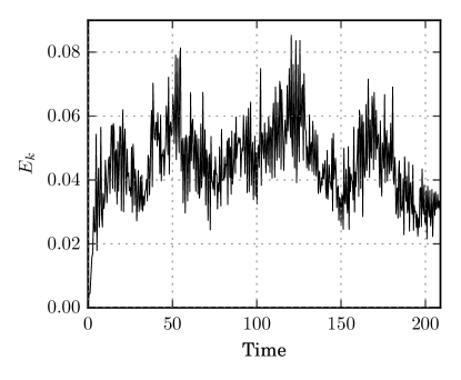
For the internal energy loss term $\mathcal{RL}$, we have tested two schemes: a spatially varying radiative loss, $\mathcal{RL}=\rho{\bf u}{\mbox{\boldmath$\cdot$}}{\bf F}$, and another that is independent of space, $\mathcal{RL}=\langle\rho{\bf u}{\mbox{\boldmath$\cdot$}}{\bf F}\rangle$. The two schemes yield indistinguishable results. Including an internal energy loss term is similar to what was done in other studies JagannathanDonzis16 ; Wangetal10 to allow total energy to remain stationary. After an initial transient, mean kinetic energy reaches a statistically stationary state as shown in Fig. 1.

Table 1: Comparison of compressibility metrics and cascade terms at different grid resolution. Low-$\zeta$ corresponds to high compressibility in the external forcing. The spatially averaged cascade terms $\langle\Lambda_{\ell}\rangle$ and $\langle\Pi_{\ell}\rangle$ are calculated using the sharp-spectral cutoff filter with $k_{\ell}=2\pi/\ell=6$. $\frac{\Delta x}{\eta}$ is the ratio of grid size to the Kolmogorov length.

Run	$N$	$\zeta$	$M_{t}$	$Re_{\lambda}$	$\frac{({\mbox{\boldmath$\nabla$}}{\mbox{\boldmath$\cdot$}}{\bf u})_{\scriptsize\mbox{rms}}}{({\mbox{\boldmath$\nabla$}}{\mbox{\boldmath$\times$}}{\bf u})_{\scriptsize\mbox{rms}}}$	$\frac{K^{d}}{K^{s}}$	$\frac{\Delta x}{\eta}$	$\left<\Pi_{\ell}\right\rangle$	$\left<\Lambda_{\ell}\right\rangle$
1	1024	0.01	0.23	65	0.50	0.74	0.23	$8.9\times 10^{-3}$	$-5.6\times 10^{-3}$
2	512	0.01	0.22	33	0.46	0.51	0.28	$6.8\times 10^{-3}$	$-4.8\times 10^{-3}$
3	512	0.6	0.33	206	0.05	0.02	1.78	$2.3\times 10^{-2}$	$-9.6\times 10^{-5}$
4	256	0.01	0.21	18	0.54	0.56	0.25	$3.6\times 10^{-3}$	$-3.1\times 10^{-3}$
5	256	0.6	0.42	150	0.04	0.01	2.1	$5.0\times 10^{-2}$	$-6.0\times 10^{-4}$
6	256	1.0	0.46	175	0.03	0.003	2.2	$5.0\times 10^{-2}$	$-3.8\times 10^{-4}$
7	128	0.01	0.20	10	0.65	0.80	0.24	$8.0\times 10^{-4}$	$-7.5\times 10^{-4}$
8	128	0.6	0.50	105	0.05	0.01	2.3	$4.0\times 10^{-2}$	$-4.0\times 10^{-4}$
9	128	1.0	0.40	95	0.03	0.01	2.0	$2.5\times 10^{-2}$	$-2.0\times 10^{-4}$

Table 1 summarizes the simulations we ran for this study and various metrics characterizing the importance of compressibility effects in each run. The turbulent Mach number is $M_{t}=\left\langle u_{i}u_{i}\right\rangle^{1/2}/\left\langle c\right\rangle$ and the Taylor Reynolds number is $Re_{\lambda}=\left\langle(u_{i}u_{i})/3\right\rangle^{1/2}\lambda/\left\langle\mu/\rho\right\rangle$. Here $c=\sqrt{\gamma p/\rho}$ is the sound speed and $\lambda=\left\langle u_{i}u_{i}\right\rangle^{1/2}/\left\langle u_{i,i}^{2}\right\rangle^{1/2}$ is the Taylor microscale. The compressibility metrics in Table 1 show the relative importance of dilatational versus solenoidal velocity modes. We use the Helmholtz decomposition, ${\bf u}={\bf u}^{d}+{\bf u}^{s}$ to obtain the dilatational ($\nabla\times\mathbf{u}^{d}=0$) and solenoidal ($\nabla\cdot\mathbf{u}^{s}=0$) components of the velocity field. The dilatational kinetic energy is $K^{d}=\left\langle\rho u_{i}^{d}u_{i}^{d}/2\right\rangle$ and the solenoidal kinetic energy is $K^{s}=\left\langle\rho u_{i}^{s}u_{i}^{s}/2\right\rangle$. Their ratio $K^{d}/K^{s}$ yields a measure of compressibility at large scales. It is well-known Federrathetal08 ; PetersenLivescu10 that the dilatational kinetic energy $K^{d}$ becomes significant when forced directly using ${\bf F}$ with a small $\zeta$. This holds, even though the low-$\zeta$ runs have a lower Mach number than high-$\zeta$ runs. The ratio $({\mbox{\boldmath$\nabla$}}{\mbox{\boldmath$\cdot$}}{\bf u})_{\scriptsize\mbox{rms}}/({\mbox{\boldmath$\nabla$}}{\mbox{\boldmath$\times$}}{\bf u})_{\scriptsize\mbox{rms}}$ yields a measure of compressibility at small scales.

The last two columns in table 1 summarize the effect of $\zeta$ on the relative importance of $\Pi$ and $\Lambda$. While the deformation work $\Pi$ is significant in all cases, baropycnal work $\Lambda$, which arises only in variable density flows, is greatly affected by the type of forcing used. At the Reynolds numbers we simulate, we find that $\Lambda$ becomes important only for low $\zeta$ when the dilatational modes are directly forced. Even at relatively high Mach numbers, $\Lambda$ remains small for high $\zeta$. We caution, however, that these observations might be Reynolds number dependent. Moreover, $\Lambda$ has been shown to dominate in non-dilatational low Mach number variable density flows Livescuetal09 ; Zhaoetal19 .

(a)

(b)

Figure 2: Momentum magnitude $|\rho\mathbf{u}|$ from (2(a)) Run 1 ($\zeta=0.01$) and (2(b)) Run 3 ($\zeta=0.6$).

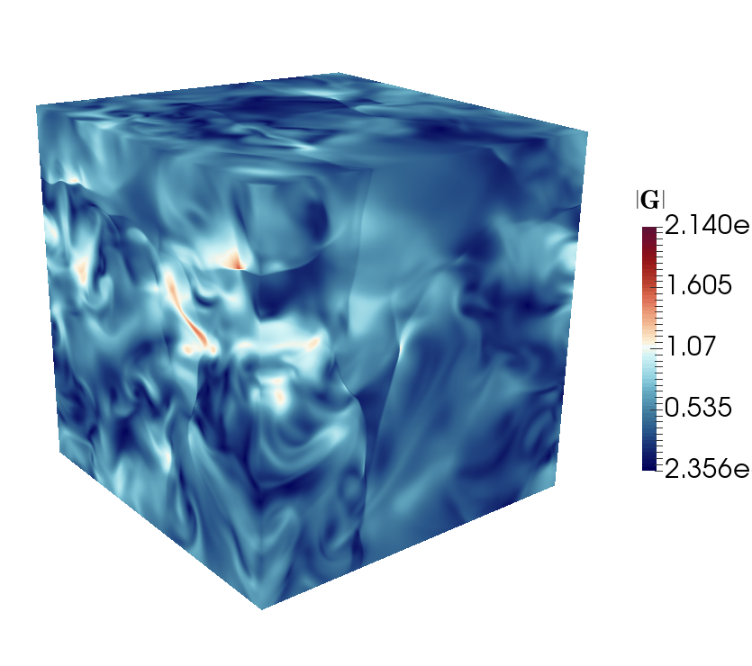
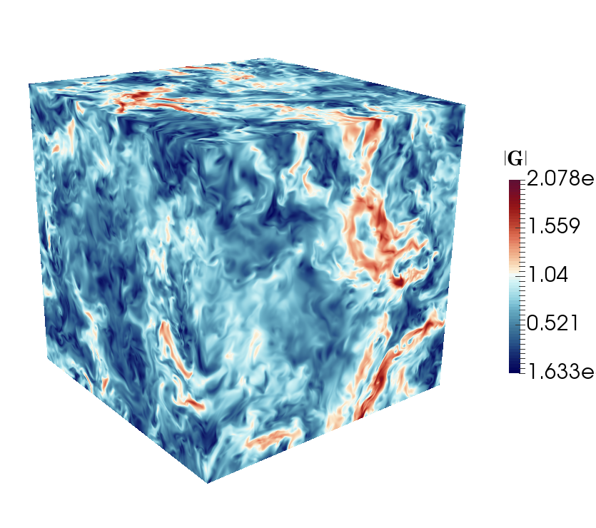
Figure 2 shows typical visualizations of the flows arising from low-$\zeta$ and high-$\zeta$ forcing. The stark qualitative difference shows the significance of dilatational forcing on the flow Federrathetal08 ; Kritsuketal10 , at least in limited resolution simulations. It has been argued Sarkaretal91 ; Shivamoggi97 ; JagannathanDonzis16 that at sufficiently high Reynolds numbers, flows forced dilatationally will produce sufficient vortical motion to resemble those forced solenoidally. Since we are primarily interested in the $\Lambda$ term here, unless stated otherwise, plots that follow will be from low-$\zeta$ simulations where $\Lambda$ is significant.

Figure 3: Spectra of velocity ($u$) and its dilatational and solenoidal ($u^{d}$ and $u^{s}$, respectively) components from Run 1. The reference dashed black lines have slopes of $-5/3$ and $-2$.

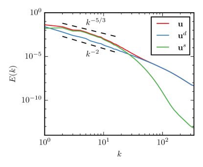
Figure 3 shows the velocity spectra in the case of highly compressive (low-$\zeta$) forcing. At intermediate scales, the spectrum of $u^{d}$ seems to follow a power law close to $k^{-2}$, which is expected for the dilatational component PetersenLivescu10 ; Federrathetal10 ; Wangetal13 . It is well-known (e.g. Federrathetal10, ; Wangetal13, ) that obtaining a clear power-law scaling of the solenoidal velocity is challenging when forcing dilatationally, even at our $1{,}024^{3}$ resolution.

Figure 4: Flux terms $\Pi_{\ell}$ and $\Lambda_{\ell}$ from Run 1, as well as their sum averaged over space and time, as a function of the filtering wavenumber $k=2\pi/\ell$. Filtering here uses the sharp-spectral filter kernel. The star superscript indicates normalization by the effective kinetic energy injection, $\varepsilon^{eff}=\varepsilon^{inj}+\langle p{\mbox{\boldmath$\nabla$}}{\mbox{\boldmath$\cdot$}}{\bf u}\rangle$.

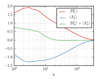
Figure 4 shows the cascade terms $\Pi_{\ell}$ and $\Lambda_{\ell}$ averaged over the domain as a function of the filter wavenumber $k$. As is the case in 3D isotropic incompressible turbulence, $\Pi_{\ell}$ is positive for all wavenumbers, transferring kinetic energy from large to small scales. On the other hand, $\Lambda_{\ell}$ is negative, effectively reducing the total amount of energy transferred across scales. This is consistent with previous studies which measured $\Lambda_{\ell}$ in homogeneous isotropic compressible turbulence Wangetal13 . Across a shock, the pressure and density gradients have the same direction and are aligned with the contracting strain eigenvector, leading to negative baropycnal work Aluie13 ; EyinkDrivas18 , thereby reducing the intensity of the cascade. Using the terminology of AlexakisBiferale18 , this is a “bi-directional cascade.” The situation is different in buoyancy driven (unstably stratified) flows, where pressure and density gradients are in opposite directions leading to positive baropycnal work Aluie13 . Within the framework of Reynolds-averaged Navier-Stokes (RANS), it has been shown that for variable density flows, such as turbulence generated by the Rayleigh-Taylor instability, the RANS equivalent of $\Lambda$ is the largest contributor to the kinetic energy cascade Livescuetal09 . We shall present our results on $\Lambda$ in buoyancy driven flows in forthcoming work Zhaoetal19 .

V Numerical Results

To quantify the pointwise agreement between baropycnal work $\Lambda$ and its nonlinear model $\Lambda_{\mbox{\small m}}$ in our DNS, we measure the correlation coefficient:

$$R_{c}=\frac{\left\langle\Lambda_{\mbox{\small m}}\Lambda\right\rangle-\left\langle\Lambda_{\mbox{\small m}}\right\rangle\left\langle\Lambda\right\rangle}{\left[\left(\left\langle\Lambda_{\mbox{\small m}}^{2}\right\rangle-\left\langle\Lambda_{\mbox{\small m}}\right\rangle^{2}\right)\left(\left\langle\Lambda^{2}\right\rangle-\left\langle\Lambda\right\rangle^{2}\right)\right]^{1/2}}.$$ (24)

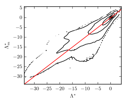
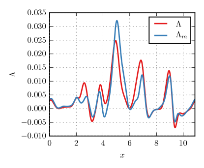
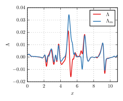
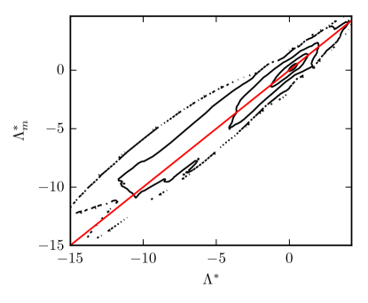
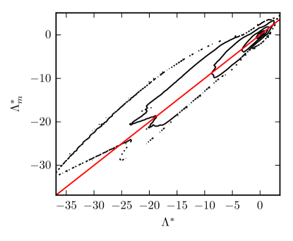
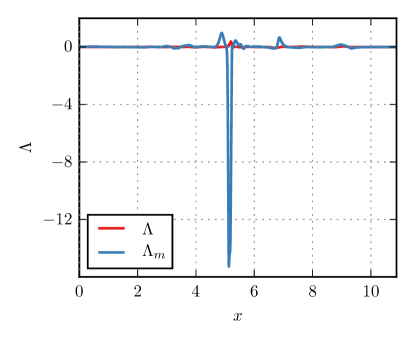
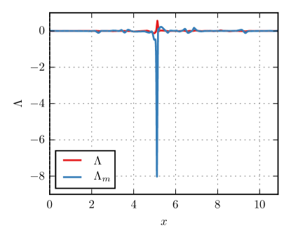
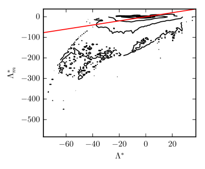
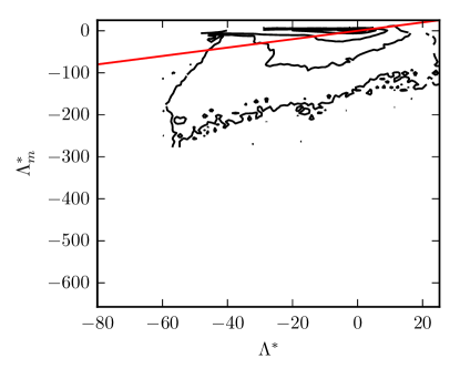
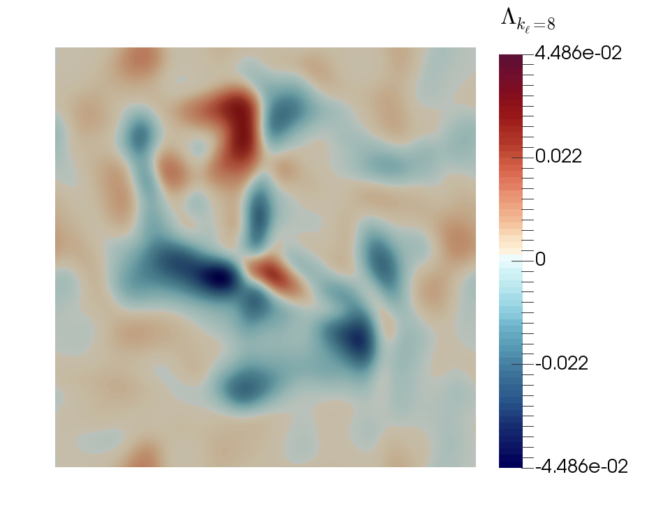
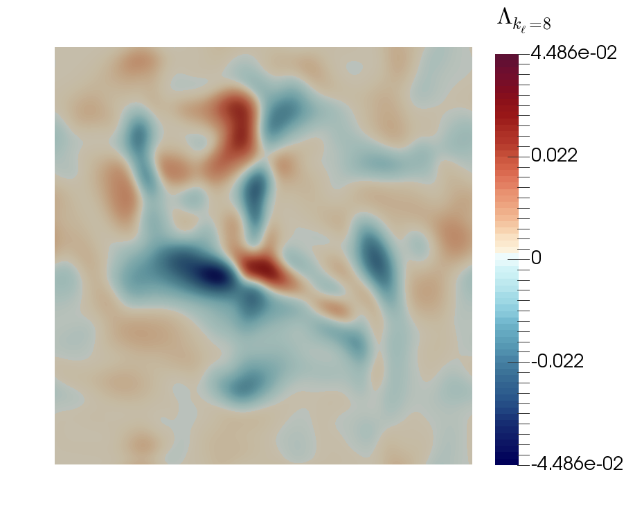
We also analyze the joint probability density function (PDF) in Figs. 5-7, and visualize $\Lambda$ and $\Lambda_{\mbox{\small m}}$ in $x$-space in Fig. 8.

Table 2: The types of filters used in calculating $\Lambda$ and $\Lambda_{\mbox{\small m}}$. The Heaviside function $H(x)=1$ for $x\geq 0$ and $H(x)=0$ for $x<0$. The correlation coefficient $R_{c}$ is shown at two scales $k_{\ell}=2\pi/\ell$.

Filter type	Kernel	$R_{c}|\,k_{\ell}=8$	$R_{c}|\,k_{\ell}=16$
Box	$G_{\ell}(\mathbf{x})=\prod_{i=1}^{3}\frac{1}{\ell}H\left(\frac{\ell}{2}-\left|x_{i}\right|\right)$	0.93	0.94
Gaussian	$G_{\ell}(\mathbf{x})=\frac{1}{\ell^{3}}\left(\frac{6}{\pi}\right)^{3/2}e^{-\frac{6\left|\mathbf{x}\right|^{2}}{\ell^{2}}}$	0.97	0.97
Sharp spectral	$\widehat{G}_{\ell}(\mathbf{k})=\prod_{i=1}^{3}H\left(\frac{2\pi}{\ell}-\left|k_{i}\right|\right)$	0.27	0.28

In our study, we use the filters defined in table 2. Both the box and Gaussian filters are positive in physical space, which is important to guarantee physical realizability of filtered quantities Vremanetal94 . On the other hand, the sharp spectral filter is not sign definite in x-space, which limits its utility in analyzing scale process in physical space.

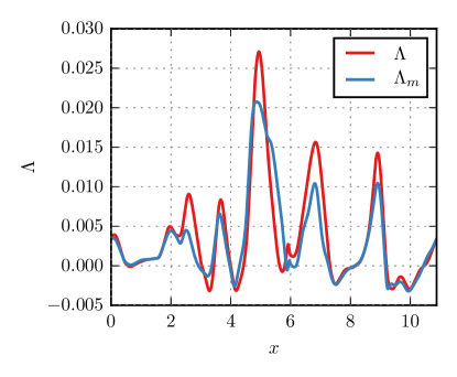
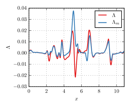
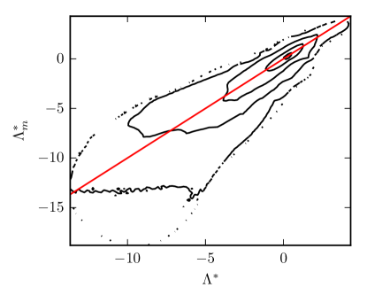
Our results indicate an excellent agreement between baropycnal work and its nonlinear model. Using either the Gaussian or Box filters, the correlation coefficients are very high, $R_{c}>0.9$, for all the length scales we analyzed. The sharp spectral filter, on the other hand, yields poor agreement. This is not surprising since the sharp spectral filter can yield negative filtered densities Aluie13 ; ZhaoAluie18 and physically unrealizable subscale stresses Vremanetal94 due to its non-positivity in x-space.

Figures 5, 6, and 7, using the box, Gaussian, and sharp spectral filters, respectively, plot $\Lambda({\bf x})$ and $\Lambda_{\mbox{\small m}}({\bf x})$ along a line in the domain to show the typical agreement between the two quantities. Also shown are the joint PDFs, which exhibit excellent linear agreement when using either the box or Gaussian kernels, but not the sharp spectral filter. Instantaneous visualizations in Figure 8 of $\Lambda({\bf x})$ and $\Lambda_{\mbox{\small m}}({\bf x})$ are consistent with the excellent statistical agreement, showing an almost perfect pointwise correlation. We note that in our dilatationally forced flows, most of the contribution to $\Lambda_{\mbox{\small m}}$ is from its straining component, $\Lambda_{SR}$, with a negligible contribution from $\Lambda_{BC}$ (see eq. (16)). This is due to the shocks which contribute mostly to $\Lambda_{SR}$. In flows dominated by baroclinicity, such as in the Rayleigh-Taylor instability, a significant contribution to $\Lambda$ comes from $\Lambda_{BC}$, as will be shown in forthcoming work Zhaoetal19 .

(a)

(b)

(c)

(d)

Figure 5: Correlation between baropycnal work and its nonlinear model from Run 1 using the box kernel with filter scale $k_{\ell}=8$ in (5(a),5(c)) and $k_{\ell}=16$ in (5(b),5(d)). Top two panels plot $\Lambda$ and $\Lambda_{\mbox{\small m}}$ along a diagonal line through the domain from a single snapshot. Lower two panels show time-averaged isocontours of the logarithm of the joint PDF between $\Lambda$ and $\Lambda_{\mbox{\small m}}$, where star superscripts indicate that means have been subtracted and the values are normalized by their variance. Straight-red lines are $y=x$. The correlation coefficients are $R_{c}=0.93$ at filter scale $k_{\ell}=8$ and $R_{c}=0.94$ at $k_{\ell}=16$. All four panels indicate excellent correlation between $\Lambda$ and $\Lambda_{\mbox{\small m}}$.

(a)

(b)

(c)

(d)

Figure 6: Same as in Fig. 5 but using the Gaussian filter. The correlation coefficients are $R_{c}=0.97$ at filter scale $k_{\ell}=8$ and $R_{c}=0.97$ at $k_{\ell}=16$. All four panels indicate excellent correlation between $\Lambda$ and $\Lambda_{\mbox{\small m}}$.

(a)

(b)

(c)

(d)

Figure 7: Same as in Fig. 5 but using the sharp-spectral filter. The correlation coefficients are $R_{c}=0.27$ at filter scale $k_{\ell}=8$ and $R_{c}=0.28$ at $k_{\ell}=16$. The correlation between $\Lambda$ and $\Lambda_{\mbox{\small m}}$ is poor when using a sharp-spectral filter due to its nonpositivity, which can yield negative filtered densities Aluie13 and physically unrealizable stresses Vremanetal94 .

(a)

(b)

Figure 8: Pointwise comparison between (a) baropycnal work and (b) its nonlinear model from a 2D slice of the 3D domain in Run 1, at one instant in time. A Gaussian kernel at scale $k_{\ell}=8$ is used. The visualizations show excellent pointwise correlation.

VI Summary

Past work Aluie11 ; Aluie13 ; EyinkDrivas18 has identified baropycnal work, $\Lambda$, as a process capable of transferring kinetic energy across scales in addition to deformation work, $\Pi$. This paper aimed at elucidating the physical mechanism by which $\Lambda$ operates.

Using scale-locality Aluie11 and a multiscale gradient expansion Eyink06a , we derived a nonlinear model, $\Lambda_{\mbox{\small m}}$, of baropycnal work. Using DNS, we showed excellent agreement between $\Lambda$ and $\Lambda_{\mbox{\small m}}$ everywhere in space and at any time, giving further empirical justification for our analysis of $\Lambda$ via its model $\Lambda_{\mbox{\small m}}$.

We found that baropycnal work operates by the baroclinic generation of vorticity, and also by strain generation due to pressure and density gradients, both barotropic and baroclinic. While the role of pressure and density gradients in generating vorticity is well recognized, their role in strain generation has been less emphasized in the literature.

As far as we know, this is the first direct demonstration of how baroclinicity enters the kinetic energy budget, which arises naturally from our scale decomposition and the identification of $\Lambda$ as a scale-transfer mechanism. Baroclinicity is often analyzed within the vorticity budget but its role in the energetics has never been obvious. The need for a scale decomposition in order for $\Lambda$ and, as a result, baroclinic energy transfer, to appear in the kinetic energy budget is similar to the scale transfer term $\Pi$, which only appears in the budget after decomposing scales due to energy conservation. In the same vein, the appearance of baroclinicity in the vorticity equation can be interpreted as being a consequence of an effective scale decomposition performed by the curl operator $\nabla$$\times$, which is a high-pass filter. Our findings here support the argument in Aluie11 ; Aluie13 to separate $\Lambda$ from pressure-dilatation, $\overline{P}{\mbox{\boldmath$\nabla$}}{\mbox{\boldmath$\cdot$}}\overline{{\bf u}}$ in compressible LES, where the two terms are often lumped together in the form of $\overline{P}{\mbox{\boldmath$\nabla$}}{\mbox{\boldmath$\cdot$}}\widetilde{{\bf u}}$.

In forthcoming work, we shall present further evidence of the excellent agreement between $\Lambda$ and $\Lambda_{\mbox{\small m}}$ using low Mach number buoyancy driven flows with significant density variability Zhaoetal19 .

References

- [1] H. Tennekes and J. L. Lumley. A First Course in Turbulence. The MIT Press, Cambridge, Massachusetts, 1972.
- [2] A Alexakis and L Biferale. Cascades and transitions in turbulent flows. Physics Reports, 767-769:1–101, November 2018.
- [3] S. B. Pope. Turbulent flows. Cambridge University Press, New York, 2000.
- [4] U. Frisch. Turbulence. The legacy of A. N. Kolmogorov. Cambridge University Press, UK, 1995.
- [5] A. Alexakis, P. D. Mininni, and A. Pouquet. Imprint of large-scale flows on turbulence. Phys. Rev. Lett., 95(26):264503, 2005.
- [6] P. D. Mininni, A. Alexakis, and A. Pouquet. Large-scale flow effects, energy transfer, and self-similarity on turbulence. Phys. Rev. E, 74(1):016303, 2006.
- [7] V Borue and S A Orszag. Local energy flux and subgrid-scale statistics in three-dimensional turbulence. Journal of Fluid Mechanics, 366(1), 1998.
- [8] Gregory L Eyink. Cascade of circulations in fluid turbulence. Physical Review E, 74(6):25, December 2006.
- [9] Gregory L Eyink. Dissipative anomalies in singular Euler flows. Physica D: Nonlinear Phenomena, 237(1):1956–1968, August 2008.
- [10] Haitao Xu, Alain Pumir, and Eberhard Bodenschatz. The pirouette effect in turbulent flows. Nature Physics, 7(9):709–712, September 2011.
- [11] G I Taylor and A E Green. Mechanism of the production of small eddies from large ones. Proceedings of the Royal Society of London Series A-Mathematical and Physical Sciences, 158(A895):0499–0521, February 1937.
- [12] G I Taylor. Production and dissipation of vorticity in a turbulent fluid. Proceedings of the Royal Society of London Series A-Mathematical and Physical Sciences, 164(A916):0015–0023, January 1938.
- [13] H. Aluie. Compressible Turbulence: The Cascade and its Locality. Phys. Rev. Lett., 106(17):174502, April 2011.
- [14] H. Aluie, S. Li, and H. Li. Conservative Cascade of Kinetic Energy in Compressible Turbulence. Astrophys. J. Lett., 751:L29, June 2012.
- [15] H. Aluie. Scale decomposition in compressible turbulence. Physica D: Nonlinear Phenomena, 247(1):54–65, March 2013.
- [16] Alexei G Kritsuk, Rick Wagner, and Michael L Norman. Energy cascade and scaling in supersonic isothermal turbulence. Journal of Fluid Mechanics, 729:1, August 2013.
- [17] Jianchun Wang, Yantao Yang, Yipeng Shi, Zuoli Xiao, X T He, and Shiyi Chen. Cascade of Kinetic Energy in Three-Dimensional Compressible Turbulence. Physical Review Letters, 110(2):214505, May 2013.
- [18] Gregory L Eyink and Theodore D Drivas. Cascades and Dissipative Anomalies in Compressible Fluid Turbulence. Physical Review X, 8(1):9, February 2018.
- [19] A. Favre. Statistical equations of turbulent gases. In Problems of hydrodynamic and continuum mechanics, SIAM, Philadelphia, pages 231–266, 1969.
- [20] S K Lele. Compressibility effects on turbulence. Annual Review of Fluid Mechanics, 26:211–254, 1994.
- [21] E. Garnier, N. Adams, and P. Sagaut. Large Eddy Simulation for Compressible Flows. Springer, Netherlands, 2009.
- [22] J O’Brien, J Urzay, M Ihme, P Moin, and A Saghafian. Subgrid-scale backscatter in reacting and inert supersonic hydrogen–air turbulent mixing layers. Journal of Fluid Mechanics, 743:554–584, 2014.
- [23] Siddhartha Mukherjee, Ahad Zarghami, Cees Haringa, Kevin van As, Saša Kenjereš, and Harry EA Van den Akker. Simulating liquid droplets: A quantitative assessment of lattice boltzmann and volume of fluid methods. International Journal of Heat and Fluid Flow, 70:59–78, 2018.
- [24] Alexei G Kritsuk, Michael L Norman, Paolo Padoan, and Rick Wagner. The statistics of supersonic isothermal turbulence. Astrophysical Journal, 665(1):416–431, 2007.
- [25] C Federrath, J Roman-Duval, R S Klessen, W Schmidt, and M M Mac Low. Comparing the statistics of interstellar turbulence in simulations and observations. Astronomy & Astrophysics, 512:A81, April 2010.
- [26] Liubin Pan, Paolo Padoan, Troels Haugbølle, and Åke Nordlund. Supernova Driving. II. Compressive Ratio In Molecular-Cloud Turbulence. The Astrophysical Journal Letters, 825(1):30, July 2016.
- [27] R Yan, R Betti, J Sanz, H Aluie, B Liu, and A Frank. Three-dimensional single-mode nonlinear ablative Rayleigh-Taylor instability. Physics of Plasmas, 23(2):022701, February 2016.
- [28] H. Zhang, R Betti, V Gopalaswamy, R Yan, and H Aluie. Nonlinear excitation of the ablative Rayleigh-Taylor instability for all wave numbers. Physical Review E, 97(1):277, January 2018.
- [29] H. Zhang, R Betti, R Yan, D Zhao, D Shvarts, and H Aluie. Self-Similar Multimode Bubble-Front Evolution of the Ablative Rayleigh-Taylor Instability in Two and Three Dimensions. Physical Review Letters, 121(18):185002, October 2018.
- [30] Johan Larsson, Stuart Laurence, Ivan Bermejo-Moreno, Julien Bodart, Sebastian Karl, and Ronan Vicquelin. Incipient thermal choking and stable shock-train formation in the heat-release region of a scramjet combustor. Part II: Large eddy simulations. Combustion and Flame, 162(4):907–920, April 2015.
- [31] Javier Urzay. Supersonic Combustion in Air-Breathing Propulsion Systems for Hypersonic Flight. Annual Review of Fluid Mechanics, 50:593–627, January 2018.
- [32] Kerry A Emanuel. An air-sea interaction theory for tropical cyclones. part i: Steady-state maintenance. Journal of the Atmospheric Sciences, 43(6):585–605, 1986.
- [33] Mark A Bourassa, Ernesto Rodriguez, and Dudley Chelton. Winds and currents mission: Ability to observe mesoscale air/sea coupling. In 2016 IEEE International Geoscience and Remote Sensing Symposium (IGARSS), pages 7392–7395. IEEE, 2016.
- [34] Luc Deike, W Kendall Melville, and Stéphane Popinet. Air entrainment and bubble statistics in breaking waves. Journal of Fluid Mechanics, 801:91–129, 2016.
- [35] Lionel Renault, James C McWilliams, and Sebastien Masson. Satellite observations of imprint of oceanic current on wind stress by air-sea coupling. Scientific reports, 7(1):17747, 2017.
- [36] C. Meneveau and J. Katz. Scale-Invariance and Turbulence Models for Large-Eddy Simulation. Ann. Rev. Fluid Mech., 32:1–32, 2000.
- [37] G. L. Eyink. Locality of turbulent cascades. Physica D, 207:91–116, 2005.
- [38] R S Strichartz. A guide to distribution theory and Fourier transforms. World Scientific Publishing Company, 2003.
- [39] Lawrence C Evans. Partial Differential Equations. Amer Mathematical Society, April 2010.
- [40] A. Leonard. Energy Cascade in Large-Eddy Simulations of Turbulent Fluid Flows. Adv. Geophys., 18:A237, 1974.
- [41] M Germano. Turbulence: the filtering approach. Journal of Fluid Mechanics, 238:325–336, 1992.
- [42] G. L. Eyink. Local energy flux and the refined similarity hypothesis. J. Stat. Phys., 78:335–351, 1995a.
- [43] Gregory L Eyink. Exact Results on Scaling Exponents in the 2D Enstrophy Cascade. Physical Review Letters, 74(1):3800–3803, May 1995b.
- [44] G. Eyink and H. Aluie. Localness of energy cascade in hydrodynamic turbulence. I. Smooth coarse graining. Phys. Fluids, 21(11):115107, November 2009.
- [45] Ugo Piomelli, William H Cabot, Parviz Moin, and Sangsan Lee. Subgrid-scale backscatter in turbulent and transitional flows. Physics of Fluids A: Fluid Dynamics, 3(7):1766–1771, 1991.
- [46] B. Vreman, B. Geurts, and H. Kuerten. Realizability conditions for the turbulent stress tensor in large-eddy simulation. J. Fluid Mech., 278:351–362, 1994.
- [47] H. Aluie and G. Eyink. Localness of energy cascade in hydrodynamic turbulence. II. Sharp spectral filter. Phys. Fluids, 21(11):115108, November 2009.
- [48] M Buzzicotti, M Linkmann, H Aluie, L Biferale, J Brasseur, and C Meneveau. Effect of filter type on the statistics of energy transfer between resolved and subfilter scales from a-priori analysis of direct numerical simulations of isotropic turbulence. Journal of Turbulence, 19:167–197, February 2018.
- [49] M. K. Rivera, W. B. Daniel, S. Y. Chen, and R. E. Ecke. Energy and Enstrophy Transfer in Decaying Two-Dimensional Turbulence. Physical Review Letters, 90(10):104502, March 2003.
- [50] S. Chen, R. E. Ecke, G. L. Eyink, X. Wang, and Z. Xiao. Physical Mechanism of the Two-Dimensional Enstrophy Cascade. Physical Review Letters, 91(21):214501, November 2003.
- [51] Jun Chen, Charles Meneveau, and Joseph Katz. Scale interactions of turbulence subjected to a straining relaxation destraining cycle. Journal of Fluid Mechanics, 562(0):123–150, September 2006.
- [52] Douglas H Kelley and Nicholas T Ouellette. Spatiotemporal persistence of spectral fluxes in two-dimensional weak turbulence. Physics of Fluids, 23(1):5101, November 2011.
- [53] M K Rivera, H Aluie, and R E Ecke. The direct enstrophy cascade of two-dimensional soap film flows. Physics of Fluids, 26(5), May 2014.
- [54] Yang Liao and Nicholas T Ouellette. Long-range ordering of turbulent stresses in two-dimensional flow. Physical Review E, 91(6):063004, June 2015.
- [55] Lei Fang and Nicholas T Ouellette. Advection and the Efficiency of Spectral Energy Transfer in Two-Dimensional Turbulence. Physical Review Letters, 117(10):104501, August 2016.
- [56] S Liu, C Meneveau, and J Katz. On the properties of similarity subgrid-scale models as deduced from measurements in a turbulent jet. Journal of Fluid Mechanics, 275:83–119, 1994.
- [57] C Meneveau. Statistics of Turbulence Subgrid-Scale Stresses - Necessary Conditions and Experimental Tests. Physics of Fluids, 6(2):815–833, February 1994.
- [58] Bo Tao, Joseph Katz, and Charles Meneveau. Statistical geometry of subgrid-scale stresses determined from holographic particle image velocimetry measurements. Journal of Fluid Mechanics, 457(0):35–78, April 2002.
- [59] Kunlun Bai, Charles Meneveau, and Joseph Katz. Experimental study of spectral energy fluxes in turbulence generated by a fractal, tree-like object. Physics of Fluids, 25(11):110810, 2013.
- [60] Yi-Chih Chow, Oguz Uzol, Joseph Katz, and Charles Meneveau. Decomposition of the spatially filtered and ensemble averaged kinetic energy, the associated fluxes and scaling trends in a rotor wake. Physics of Fluids, 17(8):085102–085102, August 2005.
- [61] Ghasem Akbari and Nader Montazerin. On the role of anisotropic turbomachinery flow structures in inter-scale turbulence energy flux as deduced from SPIV measurements. Journal of Turbulence, 14:44–70, November 2013.
- [62] H Aluie and S Kurien. Joint downscale fluxes of energy and potential enstrophy in rotating stratified Boussinesq flows. EPL (Europhysics Letters), 96(4):44006, November 2011.
- [63] Hussein Aluie, Matthew Hecht, and Geoffrey K Vallis. Mapping the Energy Cascade in the North Atlantic Ocean: The Coarse-Graining Approach. Journal of Physical Oceanography, 48(2):225–244, February 2018.
- [64] Michele Buzzicotti, Hussein Aluie, Luca Biferale, and Moritz Linkmann. Energy transfer in turbulence under rotation. Physical Review Fluids, 3(3):291, March 2018.
- [65] H. Aluie and G. Eyink. Scale Locality of Magnetohydrodynamic Turbulence. Phys. Rev. Lett., 104(8):081101, February 2010.
- [66] Hussein Aluie. Coarse-grained incompressible magnetohydrodynamics: analyzing the turbulent cascades. New Journal of Physics, January 2017.
- [67] Mahmoud Sadek and Hussein Aluie. Extracting the spectrum of a flow by spatial filtering. Physical Review Fluids, 3(12):124610, December 2018.
- [68] P Chassaing. An alternative formulation of the equations of turbulent motion for a fluid of variable density. Journal de Mecanique Theorique et Appliquee, 4:375–389, 1985.
- [69] Daniel J Bodony and Sanjiva K Lele. On using large-eddy simulation for the prediction of noise from cold and heated turbulent jets. Physics of Fluids, 17(8):085103, August 2005.
- [70] Gregory C Burton. Study of ultrahigh Atwood-number Rayleigh–Taylor mixing dynamics using the nonlinear large-eddy simulation method. Physics of Fluids, 23(4):045106, 2011.
- [71] Mona Karimi and Sharath S Girimaji. Influence of orientation on the evolution of small perturbations in compressible shear layers with inflection points. Physical Review E, 95(3), 2017.
- [72] Shigeo Kida and Steven A Orszag. Energy and spectral dynamics in forced compressible turbulence. Journal of Scientific Computing, 5(2):85–125, 1990.
- [73] Andrew W Cook and Ye Zhou. Energy transfer in Rayleigh-Taylor instability. Physical Review E, 66(2):192, August 2002.
- [74] Philipp Grete, Brian W O’Shea, Kris Beckwith, Wolfram Schmidt, and Andrew Christlieb. Energy transfer in compressible magnetohydrodynamic turbulence. Physics of Plasmas, 24(9):092311, September 2017.
- [75] Dongxiao Zhao and Hussein Aluie. Inviscid criterion for decomposing scales . Physical Review Fluids, 3:054603, May 2018.
- [76] T. Hesselberg. Die Gesetze der ausgeglichenen atmosphärischen Bewegungen. Beiträge zur Physik der freien Atmosphäre, 12:141–160, 1926.
- [77] AJ Favre, JJ Gaviglio, and RJ Dumas. Further space-time correlations of velocity in a turbulent boundary layer. Journal of Fluid Mechanics, 3(4):344–356, 1958.
- [78] Theodore D Drivas and Gregory L Eyink. An onsager singularity theorem for turbulent solutions of compressible euler equations. Communications in Mathematical Physics, 359(2):733–763, 2018.
- [79] Gregory L Eyink. Multi-scale gradient expansion of the turbulent stress tensor. Journal of Fluid Mechanics, 549(-1):159, February 2006.
- [80] J Bardina, J H Ferziger, and W C Reynolds. Improved subgrid-scale models for large-eddy simulation. American Institute of Aeronautics and Astronautics, July 1980.
- [81] David H Sharp. An overview of Rayleigh-Taylor instability. Physica D: Nonlinear Phenomena, 12(1):3–18, 1984.
- [82] P. K. Kundu and I. M. Cohen. Fluid Mechanics. Academic Press,Oxford, UK, 2008.
- [83] Christoph Federrath, Ralf S. Klessen, and Wolfram Schmidt. The density probability distribution in compressible isothermal turbulence: Solenoidal versus compressive forcing. The Astrophysical Journal Letters, 688(2):L79, 2008.
- [84] V Eswaran and SB Pope. An examination of forcing in direct numerical simulations of turbulence. Computers & Fluids, 16(3):257–278, 1988.
- [85] Shriram Jagannathan and Diego A Donzis. Reynolds and Mach number scaling in solenoidally-forced compressible turbulence using high-resolution direct numerical simulations. Journal of Fluid Mechanics, 789:669–707, February 2016.
- [86] J Wang, Wang, L.P., Z Xiao, Y Shi, and S Chen. A hybrid numerical simulation of isotropic compressible turbulence. Journal of Computational Physics, 229(13):5257–5279, 2010.
- [87] Mark R Petersen and Daniel Livescu. Forcing for statistically stationary compressible isotropic turbulence. Physics of Fluids, 22(11):116101, 2010.
- [88] D Livescu, J R Ristorcelli, R A Gore, S H Dean, W H Cabot, and A W Cook. High-Reynolds number Rayleigh-Taylor turbulence. Journal of Turbulence, 10(13):1–32, 2009.
- [89] D Zhao, R Betti, and H Aluie. The cascade in compressible rayleigh-taylor turbulence. in preparation, 2019.
- [90] A. G. Kritsuk, S. D. Ustyugov, M. L. Norman, and P. Padoan. Self-organization in Turbulent Molecular Clouds: Compressional Versus Solenoidal Modes. In Nikolai V. Pogorelov, Edouard Audit, and Gary P. Zank, editors, Numerical Modeling of Space Plasma Flows, Astronum-2009, volume 429 of Astronomical Society of the Pacific Conference Series, page 15, Sep 2010.
- [91] S Sarkar, G Erlebacher, M. Y. Hussaini, and H. O. Kreiss. The analysis and modelling of dilatational terms in compressible turbulence. Journal of Fluid Mechanics (ISSN 0022-1120), 227:473–493, June 1991.
- [92] B K Shivamoggi. Equilibrium statistical mechanics of compressible isotropic turbulence. Europhysics Letters, 38(9):657–662, 1997.