Writhe polynomials and shell moves
for virtual knots and links

Abstract.

The writhe polynomial is a fundamental invariant of an oriented virtual knot. We introduce a kind of local moves for oriented virtual knots called shell moves. The first aim of this paper is to prove that two oriented virtual knots have the same writhe polynomial if and only if they are related by a finite sequence of shell moves. The second aim of this paper is to classify oriented $2$-component virtual links up to shell moves by using several invariants of virtual links.

1. Introduction

Several invariants of classical knots correspond to local moves. For example, two classical knots have the same Arf invariant if and only if they are related by a fintie sequence of pass moves [5, 6]. Such a correspondence reveals a relationship between algebraic and geometric structures of classical knots. A similar result is known in virtual knot theory. Two virtual knots have the same odd writhe if and only if they are related by a finite sequence of $\Xi$-moves [12].

The writhe polynomial $W_{K}(t)$ of a virtual knot $K$ is a stronger invariant than the odd writhe $J(K)$: For an integer $n\neq 0$, the $n$-writhe $J_{n}(K)$ of $K$ is defined by using the index of a chord of a Gauss diagram, and the writhe polynomial and odd writhe are described by

$$W_{K}(t)=\sum_{n\neq 0}J_{n}(K)t^{n}-\sum_{n\neq 0}J_{n}(K)\mbox{ and }J(K)=\sum_{n:{\rm odd}}J_{n}(K).$$

In this paper we introduce two kinds of local moves called shell moves for virtual knots, which are defined by using Gauss diagrams as shown in Figure 1. The precise definition is given in Section 2. Then we prove the following.

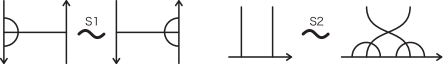
Figure 1. Shell moves

Theorem 1.1.

For two oriented virtual knots $K$ and $K^{\prime}$, the following are equivalent.

• $W_{K}(t)=W_{K^{\prime}}(t)$.

• $K$ and $K^{\prime}$ are related by a finite sequence of shell moves.

We extend the shell moves to oriented $2$-component virtual links. For an oriented $2$-component virtual link $L=K_{1}\cup K_{2}$, there are several invariants such as $\lambda(L)={\rm Lk}(K_{1},K_{2})-{\rm Lk}(K_{2},K_{1})$, $J_{n}(K_{1};L)$, $J_{n}(K_{2};L)$, and $F(L)$ whose precise definitions will be given later. By using these invariants, we classify oriented $2$-component virtual links up to shell moves. The situations are slightly different according to $\lambda(L)$.

Theorem 1.2.

Let $L=K_{1}\cup K_{2}$ and $L^{\prime}=K_{1}^{\prime}\cup K_{2}^{\prime}$ be oriented $2$-component virtual links with $\lambda(L)=\lambda(L^{\prime})=0$. Then $L$ and $L^{\prime}$ are related by a finite sequence of shell moves if and only if

• $J_{n}(K_{1};L)=J_{n}(K_{1}^{\prime};L^{\prime})$ for any $n\neq 0,1$,

• $J_{n}(K_{2};L)=J_{n}(K_{2}^{\prime};L^{\prime})$ for any $n\neq 0,1$, and

• $F(L)=F(L^{\prime})$.

Theorem 1.3.

Let $L=K_{1}\cup K_{2}$ and $L^{\prime}=K_{1}^{\prime}\cup K_{2}^{\prime}$ be oriented $2$-component virtual links with $\lambda(L)=\lambda(L^{\prime})=1$. Then $L$ and $L^{\prime}$ are related by a finite sequence of shell moves if and only if

• $J_{n}(K_{1};L)=J_{n}(K_{1}^{\prime};L^{\prime})$ for any $n\neq 0,1,-1$,

• $J_{n}(K_{2};L)=J_{n}(K_{2}^{\prime};L^{\prime})$ for any $n\neq 0,1,2$, and

• $F(L)=F(L^{\prime})$.

Theorem 1.4.

Let $L=K_{1}\cup K_{2}$ and $L^{\prime}=K_{1}^{\prime}\cup K_{2}^{\prime}$ be oriented $2$-component virtual links with $\lambda=\lambda(L)=\lambda(L^{\prime})\geq 2$. Then $L$ and $L^{\prime}$ are related by a finite sequence of shell moves if and only if

• $J_{n}(K_{1};L)=J_{n}(K_{1}^{\prime};L^{\prime})$ for any $n\neq 0,1,-\lambda,-\lambda+1$,

• $J_{n}(K_{2};L)=J_{n}(K_{2}^{\prime};L^{\prime})$ for any $n\neq 0,1,\lambda,\lambda+1$,

• $F(L)=F(L^{\prime})$, and

• $J_{1}(K_{1};L)+J_{-\lambda+1}(K_{1};L)+J_{1}(K_{2};L)+J_{\lambda+1}(K_{2};L)$

  $=J_{1}(K_{1}^{\prime};L^{\prime})+J_{-\lambda+1}(K_{1}^{\prime};L^{\prime})+J_{1}(K_{2}^{\prime};L^{\prime})+J_{\lambda+1}(K_{2}^{\prime};L^{\prime})$.

This paper is organized as follows. In Section 2, we introduce the notions of shells, shell moves, and snails in Gauss diagrams. We say that two Gauss diagrams are S-equivalent if they are related by a finite sequence of shell moves. We prove that any Gauss diagram is S-equivlanet to the one consisting of several snails. In Section 3, we study a relationship between shell moves and writhe polynomials, and prove Theorem 1.1. In Section 4, we study shell moves for oriented $2$-component virtual links, and prove that any Gauss diagram is S-equivalent to the one in standard form. In Section 5, we introduce several kinds of invariants of oriented $2$-component virtual links, and prove Theorems 1.2–1.4. In the last section, we give a relationship among the invariants in Section 5, and prove that there is no relationship other than it.

2. Shell moves

A Gauss diagram $G$ is a disjoint union of oriented circles equipped with a finite number of oriented and signed chords spanning the circles. For a chord with sign $\varepsilon$, we give signs $-\varepsilon$ and $\varepsilon$ to the initial and terminal endpoints of the chord, respectively. By definition, if two of three kinds of informations of a chord $\gamma$ — the sign of $\gamma$, the orientation of $\gamma$, and the signs of endpoints of $\gamma$ — are given, then the other is determined. We say that a chord $\gamma$ of $G$ is a self-chord if both endpoints of $\gamma$ belong to the same circle of $G$, and otherwise a nonself-chord. See Figure 2. A self-chord $\gamma$ is free if the endpoints of $\gamma$ are adjacent on the circle. A Gauss diagram is called empty if it has no chord.

Figure 2. Self- and nonself-chords of a Gauss diagram

Virtual knot theory is introduced by Kauffman [7]. A virtual link is an equivalence class of virtual link diagrams up to Reidemeister moves R1–R7. Furthermore, a virtual link diagram is an equivalence class of Gauss diagrams up to Reidemeister moves R4–R7. In this sense, a virtual link is an equivalence class of Gauss diagrams up to Reidemeister moves R1–R3 (cf. [4, 7]). In Figure 3, we illustrate Reidemeister moves R1–R3 with $\varepsilon=\pm$. Though there are many types of R3-moves with respect to orientations and signs of chords, it is enough to give just one type of R3-move as in the figure; for Polyak gives a minimal set of oriented Reidemeister moves [11].

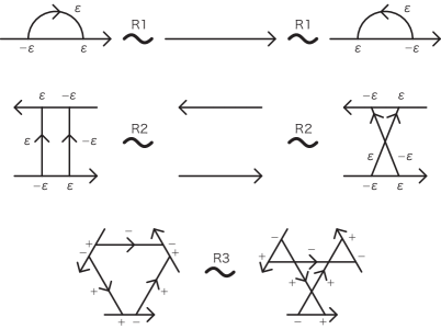
Figure 3. Reidemeister moves for Gauss diagrams

A $\mu$-component virtual link is represented by a Gauss diagram with $\mu$ circles. In particular, a $1$-component virtual link is called a virtual knot. The trivial $\mu$-component virtual link is represented by the empty Gauss diagram consisting of $\mu$ circles.

Definition 2.1.

Let $\gamma$ be a self- or nonself-chord of $G$. The shells for $\gamma$ are self-chords which surround an endpoint of $\gamma$ in parallel such that if the endpoint of $\gamma$ has positive (or negative) sign, then the orientation of shells are the same as (or opposite to) that of the circle. See Figure 4.

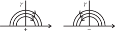
Figure 4. Shells for $\gamma$

Since the orientation of shells is determined by the sign of the endpoint of $\gamma$, we sometimes omit the orientation of $\gamma$. The notion of a shell in this paper is slightly different from that of an anklet in [9].

We introduce two kinds of deformations on Gauss diagrams as follows.

Definition 2.2.

Let $G$ be a Gauss diagram.

• A shell move S1 for $G$ is a deformation which slides a shell for a chord to another side of the chord with keeping the sign of the shell. See the left of Figure 5.

• A shell move S2 for $G$ is a deformation which changes the adjacent endpoints of a pair of chords with adding a shell to each chord as shown in the right of the figure.

• Two Gauss diagrams $G$ and $G^{\prime}$ are S-equivalent if $G$ is related to $G^{\prime}$ by a finite sequence of Reidemeister moves R1–R3 and shell moves S1 and S2. We denote it by $G\sim G^{\prime}$.

• Two oriented virtual links are S-equivalent if their Gauss diagrams are S-equivalent.

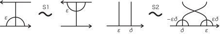
Figure 5. Shell moves S1 and S2

Let $\gamma$ be a chord of a Gauss diagram, and $k$ the sum of signs of shells for $\gamma$. We can bunch all the shells at one endpoint of $\gamma$ by using S1-moves, and then cancel them pairwise by R2-moves so that we obtain $k$ shells with positive sign for $k\geq 0$ or $-k$ shells with negative sign for $k<0$. In this sense, the algebraic number of shells for a chord is uniquely determined up to S-equivalence. See Figure 6.

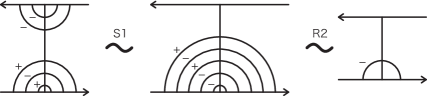
Figure 6. The algebraic number of shells for a chord

Lemma 2.3.

If two Gauss diagrams are related by a deformation $(1)$ or $(2)$ as shown in Figure 7, then they are S-equivalent. In the figure, we indicate the algebraic number of shells for each chord.

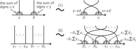
Figure 7. S-equivalent Gauss diagrams in Lemma 2.3

Proof.

(1) This is a generalization of an S2-move. We first apply S1-moves to transfer shells to the other side of each chord and then perform an S2-move. Then we apply S1-moves to get the original position of shells.

(2) This can be proved by (1) repeatedly. ∎

Corollary 2.4.

If two Gauss diagrams are related by a deformation $(1)$–$(4)$ as shown in Figure 8, then they are S-equivalent. Here, $P$ and $Q$ are portions of whole chords.

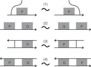
Figure 8. S-equivalent Gauss diagrams in Corollary 2.4

Proof.

(1) Since the sum of signs of endpoints of chords in $P$ is equal to $0$, the Gauss diagrams are S-equivalent by Lemma 2.3(2). We remark that although each chord in $P$ gets a pair of shells on both endpoints, they have opposite signs and can be canceled.

(2) The deformation is realized by the combination of (1)’s.

(3) We apply Lemma 2.3(2) twice as shown in Figure 9. Then we see that any new shells can be canceled by S1- and R2-moves.

(4) This can be proved similarly to (3). ∎

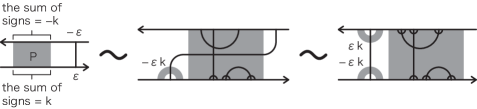
Figure 9. Proof of Corollary 2.4(3)

Definition 2.5.

Let $G$ be a Gauss diagram with $\mu$ circles $C_{1},\dots,C_{\mu}$.

• For $n\in{\mathbb{Z}}$ and $1\leq i\leq\mu$, a positive or negative $n$-snail of type $i$ is the portion of a self-chord $\gamma$ with $|n|$ shells such that $\gamma$ is spanning the circle $C_{i}$ and the sign of $\gamma$ is positive or negative, respectively, as shown in the left of Figure 10. We denote it by $+S_{i}(n)$ or $-S_{i}(n)$. We remark that $\pm S_{i}(0)$ consists of a free chord.

• For $n\in{\mathbb{Z}}$ and $1\leq i\neq j\leq\mu$, a positive or negative $n$-snail of type $(i,j)$ is the portion of a nonself-chord $\gamma$ with $|n|$ shells such that $\gamma$ is spanning between the circles $C_{i}$ and $C_{j}$ oriented from $C_{i}$ to $C_{j}$, and the sign of $\gamma$ is positive or negative, respectively, as shown in the right of the figure. We denote it by $+S_{ij}(n)$ or $-S_{ij}(n)$.

Figure 10. The $n$-snails $\varepsilon S_{i}(n)$ and $\varepsilon S_{ij}(n)$

Lemma 2.6.

If two Gauss diagrams are related by a deformation $(1)$–$(4)$ as shown in Figure 11, then they are S-equivalent.

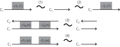
Figure 11. S-equivalent Gauss diagrams in Lemma 2.6

Proof.

(1) and (2) The positive $1$-snail $+S_{i}(1)$ is related to $-S_{i}(1)$ by an S1-move, which is eliminated by an R2-move as shown in Figure 12.

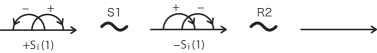
Figure 12. Proofs of Lemma 2.6(1) and (2)

(3) The concatenation of $+S_{ij}(n)$ and $-S_{ij}(n)$ is S-equivalent to that of $n$ copies of $+S_{i}(1)$ for $n>0$ or $n$ copies of canceling pairs for $n<0$ by using Lemma 2.3(2) and Corollary 2.4(1). See Figure 13, where $\varepsilon$ is the sign of $n$; that is, $n=\varepsilon|n|$. Eventually it is S-equivalent to the empty by (1) or R2-moves.

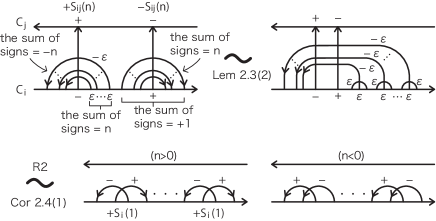
Figure 13. Proof of Lemma 2.6(3)

(4) We deform the concatenation of $+S_{i}(n)$ and $-S_{i}(n)$ as shown in Figure 14. Then we can apply the same deformation used in the proof of (3) so that it is S-equivalent to the empty. ∎

Figure 14. Proof of Lemma 2.6(4)

Proposition 2.7.

Any Gauss diagram of an oriented $\mu$-component virtual link is S-equivalent to a Gauss diagram $G$ with $\mu$ circles $C_{1},\dots,C_{\mu}$ which satisfies the following conditions. Figure 15 shows the case $\mu=3$.

• The chords of $G$ form a finite number of snails.

• There is an arc $\alpha_{i}$ on each $C_{i}$ such that all snails of type $i$ spans $\alpha_{i}$.

• All snails of type $(i,j)$ spans $(C_{i}\setminus\alpha_{i})\cup(C_{j}\setminus\alpha_{j})$ in parallel.

• There is no snails $\pm S_{i}(0)$ or $\pm S_{i}(1)$ for any $i$.

• There is no pair of snails $+S_{i}(n)$ and $-S_{i}(n)$ for any $i$ and $n$.

• There is no pair of snails $+S_{ij}(n)$ and $-S_{ij}(n)$ for any $i\neq j$ and $n$.

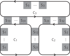
Figure 15. A Gauss diagram with three circles

Proof.

For each self-chord $\gamma$ spanning $C_{i}$, we slide the initial endpoint of $\gamma$ along $C_{i}$ with respect to the orientation of $C_{i}$ by using Lemma 2.3(1) so that the initial endpoint of $\gamma$ is adjacent to the terminal with some shells. Then we obtain a snail $\pm S_{i}(n)$ on $C_{i}$ for some $n$. By Corollary 2.4(1) and (2), we may assume that all snails span $\alpha_{i}$, and the endpoints of nonself-chords with shells on $C_{i}$ are contained in $C_{i}\setminus\alpha_{i}$. For the nonself-chords with shells between $C_{i}$ and $C_{j}$, we move the endpoints on $C_{i}\setminus\alpha_{i}$ by Lemma 2.3(1) to obtain parallel snails of type $(i,j)$. Therefore we have the conditions (i)–(iii).

The conditions (iv)–(vi) are derived from Lemma 2.6 directly. ∎

We remark that by Corollary 2.4(2) and (4), the Gauss diagrams which are different in the position of snails are all S-equivalent.

3. The case $\mu=1$

Throughout this section, we consider an oriented virtual knot $K$ and its Gauss diagram $G$ consisting of a single circle $C$.

Let $P_{i}$ $(1\leq i\leq k)$ be portions of whole chords on $C$. We denote by $\left(\sum_{i=1}^{k}P_{i}\right)$ the Gauss diagram consisting of the concatenation of $P_{i}$’s. See Figure  16.

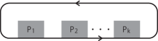
Figure 16. The Gauss diagram $\left(\sum_{i=1}^{k}P_{i}\right)$

For integers $a$ and $n$, we denote by $aS(n)$ the concatenation of $a$ copies of $+S(n)$ for $a>0$, $-a$ copies of $-S(n)$ for $a<0$, and the empty for $a=0$. Here, we abbreviate $\pm S_{1}(n)$ to $\pm S(n)$ for simplicity. Then by Proposition 2.7 we have the following.

Lemma 3.1.

Any Gauss daigram of $K$ is $S$-equivalent to $\left(\sum_{n\neq 0,1}a_{n}S(n)\right)$ for some $a_{n}\in{\mathbb{Z}}$. $\Box$

Let $G$ be a Gauss diagram of a virtual knot $K$, and $\gamma$ a chord of $G$. The endpoints of $\gamma$ divide the circle $C$ into two arcs. Let $\alpha$ be the arc oriented from the initial endpoint of $\gamma$ to the terminal. The index of $\gamma$ is the sum of signs of endpoints of chords on $\alpha$, and denoted by ${\rm Ind}(\gamma)\in{\mathbb{Z}}$ (cf. [1, 8, 12]).

For each integer $n$, we denote by $J_{n}(G)$ the sum of signs of all chords $\gamma$ with ${\rm Ind}(\gamma)=n$. If $n\neq 0$, then $J_{n}(G)$ does not depend on a particular choice of $G$ of $K$ [12]. It is called the $n$-writhe of $K$ and denoted by $J_{n}(K)$. The writhe polynomial of $K$ is defined by

$$W_{K}(t)=\sum_{n\neq 0}J_{n}(K)t^{n}-\sum_{n\neq 0}J_{n}(K)\in{\mathbb{Z}}[t,t^{-1}].$$

This invariant is introduced in several papers [2, 8, 12] independently. A characterization of $W_{K}(t)$ is given as follows.

Theorem 3.2 ([12]).

For a Laurent polynomial $f(t)\in{\mathbb{Z}}[t,t^{-1}]$, the following are equivalent.

• There is a virtual knot $K$ such that $W_{K}(t)=f(t)$.

• $f(1)=f^{\prime}(1)=0$.

In particular, it holds that $J_{1}(K)=-\sum_{n\neq 0,1}nJ_{n}(K)$. $\Box$

Example 3.3.

Figure 17 shows an example of a Gauss diagram $G$ with five chords whose indices are surrounded by boxes. Let $K$ be the oriented virtual knot presented by $G$. It holds that

$$J_{n}(K)=\left\{\begin{array}[]{rl}1&(n=3,-1),\\ -2&(n=1),\mbox{ and}\\ 0&(n\neq 3,1,0,-1).\end{array}\right.$$

Therefore we have we have $W_{K}(t)=t^{-1}-2t+t^{3}$.

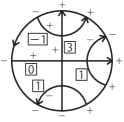
Figure 17. A Gauss diagram with five chords

Lemma 3.4.

Let $\gamma$ be a chord of $G$.

• If $\gamma$ is a shell, then we have ${\rm Ind}(\gamma)=1$.

• If $\gamma$ is not a shell, then the index does not change under S-moves.

Proof.

(i) Since the sum of signs of endpoints of all chords is equal to $0$, it follows from the definition of a shell.

(ii) This follows from the definition of the index of a chord. We remark that the indices of chords $\gamma$ and $\gamma^{\prime}$ as shown in Figure 18 do not change under an S2-move. ∎

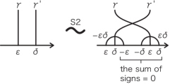
Figure 18. A shell move S2

Lemma 3.5.

Let $K$ be an oriented virtual knot.

• The $n$-writhe $J_{n}(K)$ $(n\neq 0)$ is invariant under S-moves, and hence so is the writhe polynomial $W_{K}(t)$.

• If $K$ is presented by a Gauss diagram given in Lemma 3.1, then we have

  $$W_{K}(t)=\sum_{n\neq 0,1}a_{n}t^{n}-\left(\sum_{n\neq 0,1}na_{n}\right)t+\sum_{n\neq 0,1}(n-1)a_{n}.$$

Proof.

(i) If a chord $\gamma$ satisfies ${\rm Ind}(\gamma)\neq 1$, then the index of $\gamma$ does not change under S-moves, and hence $J_{n}(K)$ is invariant for $n\neq 0,1$ by Lemma 3.4. Furthermore, since $J_{1}(K)=-\sum_{n\neq 0,1}nJ_{n}(K)$ by Theorem 3.2, $J_{1}(K)$ is also invariant under S-moves.

(ii) Since $J_{n}(K)=a_{n}\ (n\neq 0,1)$ and $J_{1}(K)=-\sum_{n\neq 0,1}na_{n}$ hold, we have the conclusion. ∎

Theorem 3.6.

Let $K$ and $K^{\prime}$ be oriented virtual knots. If $W_{K}(t)=W_{K^{\prime}}(t)$ holds, then $K$ and $K^{\prime}$ are S-equivalent.

Proof.

By Lemma 3.1, any Gauss diagrams of $K$ and $K^{\prime}$ are S-equivalent to Gauss diagrams

$$G=\left(\sum_{n\neq 0,1}a_{n}S(n)\right)\mbox{ and }G^{\prime}=\left(\sum_{n\neq 0,1}a_{n}^{\prime}S(n)\right),$$

respectively.

By Lemma 3.5(ii) and the assumption, we obtain $a_{n}=a_{n}^{\prime}$ for any $n\neq 0,1$, and hence $G=G^{\prime}$.

∎

Proof of Theorem 1.1.

This follows from Lemma 3.5(i) and Theorem 3.6. ∎

Remark 3.7.

We can give an alternative proof of Theorem 3.2 as follows: A Laurent polynomial $f(t)=\sum_{n\in{\mathbb{Z}}}a_{n}t^{n}$ satisfies $f(1)=f^{\prime}(1)=0$ if and only if $a_{1}=-\sum_{n\neq 0,1}na_{n}$ and $a_{0}=\sum_{n\neq 0,1}(n-1)a_{n}$, that is,

$$f(t)=\sum_{n\neq 0,1}a_{n}t^{n}-\left(\sum_{n\neq 0,1}na_{n}\right)t+\sum_{n\neq 0,1}(n-1)a_{n}.$$

This polynomial is equal to $W_{K}(t)$ given in Lemma 3.5(ii).

Remark 3.8.

The Jones polynomial of a virtual knot is invariant under an S1-move but not under an S2-move. The proof is easy and will be left to the reader.

4. The case $\mu=2$ (geometric part)

Throughout Sections 4–6, we consider an oriented $2$-component virtual link $L=K_{1}\cup K_{2}$ and its Gauss diagram $G$ consisting of a pair of circles $C_{1}$ and $C_{2}$. By Proposition 2.7 we have the following.

Lemma 4.1.

Any Gauss daigram of $L$ is $S$-equivalent to a Gauss diagram

$$\left(\sum_{n\neq 0,1}a_{n}S_{1}(n),\sum_{n\neq 0,1}b_{n}S_{2}(n);\sum_{m\in{\mathbb{Z}}}c_{m}S_{12}(m),\sum_{m\in{\mathbb{Z}}}d_{m}S_{21}(m)\right)$$

for some integers $a_{n},b_{n}$ $(n\neq 0,1)$ and $c_{m},d_{m}$ $(m\in{\mathbb{Z}})$ as shown in Figure 22. Here, the entries present the concatenations of snails of type $1$, $2$, $(1,2)$, and $(2,1)$, respectively. $\Box$

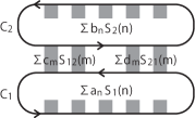
Figure 19. A Gauss diagram of an oriented $2$-component virtual link

A nonself-chord of $G$ is called of type $(i,j)$ for $1\leq i\neq j\leq 2$ if it is oriented from $C_{i}$ to $C_{j}$; that is, the initial and terminal endpoints belong to $C_{i}$ and $C_{j}$, respectively. The $(i,j)$-linking number of $L$, denoted by ${\rm Lk}(K_{i},K_{j})$, is the sum of signs of all nonself-chords of type $(i,j)$, which does not depend on a particular choice of $G$ for $L$. The virtual linking number of $L$ is defined by $\lambda(L)={\rm Lk}(K_{1},K_{2})-{\rm Lk}(K_{2},K_{1})$ [10] (cf. [3]).

Lemma 4.2.

Let $L=K_{1}\cup K_{2}$ be an oriented $2$-component virtual link.

• The linking numbers ${\rm Lk}(K_{1},K_{2})$ and ${\rm Lk}(K_{2},K_{1})$ are invariant under S-moves, and hence so is the virtual linking number $\lambda(L)$.

• If $L$ is presented by a Gauss diagram given in Lemma 4.1, then we have ${\rm Lk}(K_{1},K_{2})=\sum_{m\in{\mathbb{Z}}}c_{m}$ and ${\rm Lk}(K_{2},K_{1})=\sum_{m\in{\mathbb{Z}}}d_{m}$.

Proof.

(i) The invariance under S-moves is obtained by definition directly.

(ii) Each snail $\pm S_{ij}(m)$ contains the unique nonself-chord with sign $\pm 1$. ∎

For simplicity, we use the notation $\lambda=\lambda(L)$.

Lemma 4.3.

For any Gauss diagram of $L$, we have the following.

• The sum of signs of endpoints of chords on $C_{1}$ is equal to $-\lambda$.

• The sum of signs of endpoints of chords on $C_{2}$ is equal to $\lambda$.

Proof.

(i) Each self-chord of type $1$ does not contribute to the sum of signs on $C_{1}$. On the other hand, each nonself-chord of type $(1,2)$ (or type $(2,1))$ with sign $\varepsilon$ contributes to the sum on $C_{1}$ by $-\varepsilon$ (or $\varepsilon$). Therefore the sum on $C_{1}$ is equal to $-{\rm Lk}(K_{1},K_{2})+{\rm Lk}(K_{2},K_{1})=-\lambda$.

(ii) By changing the roles between $K_{1}$ and $K_{2}$ in (i), the sum on $C_{2}$ is equal to $-{\rm Lk}(K_{2},K_{1})+{\rm Lk}(K_{1},K_{2})=\lambda$. ∎

Lemma 4.4.

We have the following S-equivalent Gauss diagrams.

• $\left(P+S_{1}(-\lambda),Q;\sum c_{m}S_{12}(m),\sum d_{m}S_{21}(m)\right)$

  $\sim\left(P,Q;\sum c_{m}S_{12}(m-1),\sum d_{m}S_{21}(m+1)\right)$.

• $\left(P+S_{1}(-\lambda+1),Q;\sum c_{m}S_{12}(m),\sum d_{m}S_{21}(m)\right)$

  $\sim\left(P,Q;\sum c_{m}S_{12}(m-1),\sum d_{m}S_{21}(m+1)\right)$.

• $\left(P,Q+S_{2}(\lambda);\sum c_{m}S_{12}(m),\sum d_{m}S_{21}(m)\right)$

  $\sim\left(P,Q;\sum c_{m}S_{12}(m+1),\sum d_{m}S_{21}(m-1)\right)$.

• $\left(P,Q+S_{2}(\lambda+1);\sum c_{m}S_{12}(m),\sum d_{m}S_{21}(m)\right)$

  $\sim\left(P,Q;\sum c_{m}S_{12}(m+1),\sum d_{m}S_{21}(m-1)\right)$.

Proof.

(i) In the Gauss diagram in the left hand side, let $\gamma$ be the self-chord of $+S_{1}(-\lambda)$ other than the shells. We move the terminal endpoint of $\gamma$ around $C_{1}$ with respect to the orientation of $C_{1}$.

By Lemmas 2.3 and 4.3, the terminal endpoint of $\gamma$ gets shells such that the sum of signs is equal to $-\lambda$. Since the algebraic number of shells for $\gamma$ is equal to $0$, $\gamma$ becomes a free chord which can be removed by an R1-move. See Figure 20.

On the other hand, each snail $\pm S_{12}(m)$ changes into $\pm S_{12}(m-1)$ after the terminal endpoint of $c$ passes, and $\pm S_{21}(m)$ changes into $\pm S_{21}(m+1)$.

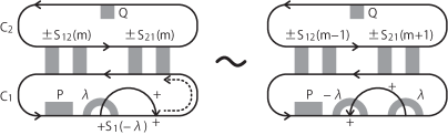
Figure 20. Proof of Lemma 4.4(i)

(ii) The proof is almost the same as that of (i). The difference is that the algebraic number of shells for $\gamma$ after moving the terminal endpoint of $\gamma$ around $C_{1}$ is equal to $-1$, the snail $+S_{1}(-\lambda+1)$ changes into a pair of chords which can be canceled by an R2-move.

(iii) and (iv) These are obtained from (i) and (ii) by changing the roles of first and second components. ∎

Lemma 4.5.

For any integer $M$, a Gauss diagram

$$\left(P,Q;\sum_{m\in{\mathbb{Z}}}c_{m}S_{12}(m),\sum_{m\in{\mathbb{Z}}}d_{m}S_{21}(m)\right)$$

is S-equivalent to the following.

• $\displaystyle{\left(P,Q;c_{M}S_{12}(M-c_{M}+\lambda)+\sum_{m\neq M}c_{m}S_{12}(m-c_{M}),\sum_{m\in{\mathbb{Z}}}d_{m}S_{21}(m+c_{M})\right)}$.

• $\displaystyle{\left(P,Q;c_{M}S_{12}(M+c_{M}-\lambda)+\sum_{m\neq M}c_{m}S_{12}(m+c_{M}),\sum_{m\in{\mathbb{Z}}}d_{m}S_{21}(m-c_{M})\right)}$.

• $\displaystyle{\left(P,Q;\sum_{m\in{\mathbb{Z}}}c_{m}S_{12}(m+d_{M}),d_{M}S_{21}(M-d_{M}-\lambda)+\sum_{m\neq M}d_{m}S_{21}(m-d_{M})\right)}$.

• $\displaystyle{\left(P,Q;\sum_{m\in{\mathbb{Z}}}c_{m}S_{12}(m-d_{M}),d_{M}S_{21}(M+d_{M}+\lambda)+\sum_{m\neq M}d_{m}S_{21}(m+d_{M})\right)}$.

Proof.

(i) We move the endpoints of $c_{M}S_{12}(M)$ around $C_{1}$ with respect to the orientation of $C_{1}$. See Figure 21. By Lemmas 2.3 and 4.3, $c_{M}S_{12}(M)$ changes into $c_{M}S_{12}(M-c_{M}+\lambda)$, and $c_{m}S_{12}(m)$ $(m\neq M)$ and $d_{m}S_{21}(m)$ change into $c_{m}S_{12}(m-c_{M})$ and $d_{m}S_{21}(m+c_{M})$, respectively.

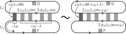
Figure 21. Proof of Lemma 4.5(i)

(ii) It is sufficient to move the endpoints of $c_{M}S_{12}(M)$ around $C_{1}$ with respect to the reverse orientation of $C_{1}$.

(iii) and (iv) These are obtained from (i) and (ii) by changing the roles of first and second components. ∎

If $\lambda(L)<0$, then by switching the roles of $K_{1}$ and $K_{2}$, the case reduces to $\lambda(L)>0$. In what follows, we may assume that $\lambda(L)\geq 0$.

Proposition 4.6.

Let $G$ be a Gauss diagram of $L$.

• If $\lambda\geq 1$, then

  $\displaystyle{G\sim\left(\sum_{n\neq 0,1,-\lambda,-\lambda+1}a_{n}S_{1}(n),\sum_{n\neq 0,1,\lambda,\lambda+1}b_{n}S_{2}(n);\right.}$

  $\displaystyle{\left.\sum_{m=0}^{\lambda-1}c_{m}S_{12}(p+m),\sum_{m=0}^{\lambda-1}d_{m}S_{21}(-p-m)\right)}$

  for some integers $a_{n}$ $(n\neq 0,1,-\lambda,-\lambda+1)$, $b_{n}$ $(n\neq 0,1,\lambda,\lambda+1)$, $c_{m},d_{m}$ $(0\leq m\leq\lambda-1)$, and $p$.

• In particular, if $\lambda=1$, then

  $$G\sim\left(\sum_{n\neq 0,1,-1}a_{n}S_{1}(n),\sum_{n\neq 0,1,2}b_{n}S_{2}(n);c_{0}S_{12}(0),d_{0}S_{21}(0)\right)$$

  for some integers $a_{n}$ $(n\neq 0,1,-1)$, $b_{n}$ $(n\neq 0,1,2)$, $c_{0}$, and $d_{0}$.

Proof.

(i) We may start a Gauss diagram of the form in Lemma 4.1. By Lemma 4.4, we can remove the snails $\pm S_{1}(-\lambda)$ and $\pm S_{1}(-\lambda+1)$ from the first entry, and $\pm S_{2}(\lambda)$ and $\pm S_{2}(\lambda+1)$ from the second entry. Moreover, by Lemma 4.5, we see that there are integers $p$ and $q$ such that it is S-equivalent to a Gauss diagram

$$G^{\prime}=\left(P,Q;\sum_{m=0}^{\lambda-1}c_{m}S_{12}(p+m),\sum_{m=0}^{\lambda-1}d_{m}S_{21}(q-m)\right)$$

with

$$P=\sum_{n\neq 0,1,-\lambda,-\lambda+1}a_{n}S_{1}(n)\mbox{ and }Q=\sum_{n\neq 0,1,\lambda,\lambda+1}b_{n}S_{2}(n)$$

for some integers $a_{n}$, $b_{n}$, $c_{m}$, $d_{m}$, $p$, and $q$.

Now we put $h(G^{\prime})=p+q$. If $h(G^{\prime})=0$, then the proof is completed. Assume that $h(G^{\prime})>0$. The case $h(G^{\prime})<0$ can be similarly proved. By applying Lemma 4.5(ii) for $G^{\prime}$ with $M=p+\lambda-1$, $G$ is S-equivalent to the Gauss diagram $G^{\prime\prime}$ given by

$\displaystyle{\left(P,Q;c_{p+\lambda-1}S_{12}(p+c_{p+\lambda-1}-1)+\sum_{m=0}^{\lambda-2}c_{m}S_{12}(p+c_{p+\lambda-1}+m),\right.}$

$\displaystyle{\left.\sum_{m=0}^{\lambda-1}d_{m}S_{21}(q-c_{p+\lambda-1}-m)\right)}.$

Since it holds that

$$h(G^{\prime\prime})=(p+c_{p+\lambda-1}-1)+(q-c_{p+\lambda-1})=p+q-1=h(G^{\prime})-1,$$

by repeating this modification suitably, we finally obtain a Gauss diagram $G^{\prime\prime\prime}$ with $h(G^{\prime\prime\prime})=0$ which is S-equivalent to $G$.

(ii) By (i), $G$ is S-equivalent to a Gauss diagram

$$\left(\sum_{n\neq 0,1,-1}a_{n}S_{1}(n),\sum_{n\neq 0,1,2}b_{n}S_{2}(n);c_{0}S_{12}(p),d_{0}S_{21}(-p)\right)$$

for some integers $a_{n}$ $(n\neq 0,1,-1)$, $b_{n}$ $(n\neq 0,1,2)$, $c_{0}$, and $d_{0}$. By Lemma 4.4(ii) with $\lambda=1$, we can take $p=0$. ∎

We remark that by Lemma 4.2(ii) we have $c_{0}={\rm Lk}(K_{1},K_{2})$ and $d_{0}={\rm Lk}(K_{2},K_{1})$ in Proposition 4.6(ii).

Lemma 4.7.

We have the following S-equivalent Gauss diagrams.

• If $\lambda=0$, then

  $\displaystyle{\left(P,Q;\sum_{m\in{\mathbb{Z}}}c_{m}S_{12}(m),\sum_{m\in{\mathbb{Z}}}d_{m}S_{21}(m)\right)}$

  $\displaystyle{\sim\left(P,Q;\sum_{m\in{\mathbb{Z}}}c_{m}S_{12}(m+k),\sum_{m\in{\mathbb{Z}}}d_{m}S_{21}(m-k)\right)}$

  for any $k\in{\mathbb{Z}}$.

• If $\lambda\geq 2$, then

  $\displaystyle{\left(P,Q;\sum_{m=0}^{\lambda-1}c_{m}S_{12}(p+m),\sum_{m=0}^{\lambda-1}d_{m}S_{21}(-p-m)\right)}$

  $\displaystyle{\sim\left(P,Q;\sum_{m=0}^{\lambda-1}c_{m}^{\prime}S_{12}(p^{\prime}+m),\sum_{m=0}^{\lambda-1}d_{m}^{\prime}S_{21}(-p^{\prime}-m)\right),}$

  where

  $$\left\{\begin{array}[]{l}(c_{0}^{\prime},\dots,c_{\lambda-k-1}^{\prime},c_{\lambda-k}^{\prime},\dots,c_{\lambda-1}^{\prime})=(c_{k},\dots,c_{\lambda-1},c_{0},\dots,c_{k-1}),\\ (d_{0}^{\prime},\dots,d_{\lambda-k-1}^{\prime},d_{\lambda-k}^{\prime},\dots,d_{\lambda-1}^{\prime})=(d_{k},\dots,d_{\lambda-1},d_{0},\dots,d_{k-1}),\end{array}\right.$$

  and $p^{\prime}=p+k-\sum_{i=0}^{k-1}(c_{i}-d_{i})$ for any $k$ with $1\leq k\leq\lambda-1$.

Proof.

(i) Since $\lambda=0$, this follows from Lemma 4.4 immediately.

(ii) It is sufficient to prove the case of $k=1$. By Lemma 4.5(i), the left hand side is S-equivalent to

$$\left(P,Q;\sum_{m=1}^{\lambda-1}c_{m}S_{12}(p-c_{0}+m)+c_{0}S_{12}(p-c_{0}+\lambda),\sum_{m=0}^{\lambda-1}d_{m}S_{21}(-p+c_{0}-m)\right).$$

Furthermore, by Lemma 4.5(iii), this is S-equivalent to

$\displaystyle{\left(P,Q;\sum_{m=1}^{\lambda-1}c_{m}S_{12}(p-c_{0}+d_{0}+m)+c_{0}S_{12}(p-c_{0}+d_{0}+\lambda),\right.}$

$\displaystyle{\left.\sum_{m=1}^{\lambda-1}d_{m}S_{21}(-p+c_{0}-d_{0}-m)+d_{0}S_{21}(-p+c_{0}-d_{0}-\lambda)\right)}$

$\displaystyle{=\left(P,Q;\sum_{m=0}^{\lambda-2}c_{m+1}S_{12}(p^{\prime}+m)+c_{0}S_{12}(p^{\prime}+\lambda-1),\right.}$

$\displaystyle{\left.\sum_{m=0}^{\lambda-2}d_{m+1}S_{21}(-p^{\prime}-m)+d_{0}S_{21}(-p^{\prime}-\lambda+1)\right),}$

where $p^{\prime}=p+1-c_{0}+d_{0}$. This is coincident with the right hand side in the case of $k=1$. ∎

5. The case $\mu=2$ (algebraic part)

Let $G$ be a Gauss diagram of an oriented $2$-component virtual link $L=K_{1}\cup K_{2}$. The index of a self- or nonself-chord $\gamma$ of $G$ is defined as follows.

• Let $\gamma$ be a self-chord spanning a circle $C_{i}$. The index of $\gamma$ in $G$ is the sum of signs of endpoints of self- and nonself-chords on the arc of $C_{i}$ oriented from the initial endpoint of $\gamma$ to the terminal (cf. [13]). We denote it by ${\rm Ind}^{\prime}(\gamma)$.

• Fix a nonself-chord $\gamma_{0}$ of $G$. Let $\gamma$ be a nonself-chord of type $(i,j)$. Let $\alpha$ be the arc on $C_{i}$ oriented from the initial endpoint of $\gamma$ to an endpoint of $\gamma_{0}$, and $\beta$ the arc on $C_{j}$ oriented from another endpoint of $\gamma_{0}$ to the terminal endpoint of $\gamma$. See the left of Figure 22. The index of $\gamma$ with respect to $\gamma_{0}$ in $G$ is the sum of signs of endpoints of self- and nonself-chords on $\alpha\cup\beta$ (cf. [2]). We denote it by ${\rm Ind}^{\prime}(\gamma;\gamma_{0})$.

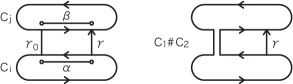
Figure 22. The index of a nonself-chord

Remark 5.1.

We have two remarks.

• For a self-chord $\gamma$ spanning a circle $C_{i}$, the index ${\rm Ind}^{\prime}(\gamma)$ is generally not equal to the original index ${\rm Ind}(\gamma)$ in Section 3 restricted to the Gauss diagram consisting of the circle $C_{i}$ with self-chords spanning $C_{i}$.

• For a nonself-chord $\gamma$ of type $(i,j)$, the index ${\rm Ind}^{\prime}(\gamma;\gamma_{0})$ is equal to the index ${\rm Ind}(\gamma)$ in the Gauss diagram consisting of the circle $C_{1}\#C_{2}$ obtained from $G$ by surgery along $\gamma_{0}$. See the right of Figure 22.

Lemma 5.2.

Let $\gamma$ be a chord of $G$.

• If $\gamma$ is a shell spanning $C_{1}$, then ${\rm Ind}^{\prime}(\gamma)=1,-\lambda+1$.

• If $\gamma$ is a shell spanning $C_{2}$, then ${\rm Ind}^{\prime}(\gamma)=1,\lambda+1$.

• If $\gamma$ is not a shell, then the index does not change under S-moves.

Proof.

This follows from the definition of the index immediately. ∎

For an integer $n$, we denote by $J_{n}^{i}(G)$ $(i=1,2)$ the sum of signs of all self-chords $\gamma$ spanning $C_{i}$ with ${\rm Ind}^{\prime}(\gamma)=n$. It is known in [13] that $J_{n}^{1}(G)$ is independent of a particular choice of $G$ for $n\neq 0,-\lambda$. It is called the $n$-writhe of $K_{1}$ in $L$ and denoted by $J_{n}(K_{1};L)$ for $n\neq 0,-\lambda$. Similarly $J_{n}^{2}(G)$ is independent of a particular choice of $G$ for $n\neq 0,\lambda$. It is called the $n$-writhe of $K_{2}$ in $L$ and denoted by $J_{n}(K_{2};L)$ for $n\neq 0,\lambda$. We remark that the index of a free chord spanning $C_{1}$ (or $C_{2}$) is equal to $0$ or $-\lambda$ (or $0$ or $\lambda$).

Example 5.3.

We consider the Gauss diagram

$$G=(2S_{1}(2)-S_{1}(3),2S_{2}(-1);S_{12}(0)+S_{12}(-1)+S_{12}(4),2S_{21}(2)-S_{21}(3))$$

as shown in Figure 23. Let $L=K_{1}\cup K_{2}$ be the oriented $2$-component virtual link presented by $G$. We have

$${\rm Lk}(K_{1},K_{2})=3,\ {\rm Lk}(K_{2},K_{1})=1,\mbox{ and }\lambda(L)=2.$$

Furthermore, it holds that

$$J_{n}(K_{1};L)=\left\{\begin{array}[]{rl}-5&(n=-1),\\ 2&(n=2),\\ -1&(n=3),\\ 0&(\mbox{otherwise}),\end{array}\right.\mbox{ and }J_{n}(K_{2};L)=\left\{\begin{array}[]{rl}2&(n=-1),\\ 1&(n=1,3),\\ 0&(\mbox{otherwise}).\end{array}\right.$$

Figure 23. The Gauss diagram in Example 5.3

Lemma 5.4.

Let $L=K_{1}\cup K_{2}$ be an oriented $2$-component virtual link.

• The $n$-writhes

  • $J_{n}(K_{1};L)\in{\mathbb{Z}}$ $(n\neq 0,1,-\lambda,-\lambda+1)$ and

  • $J_{n}(K_{2};L)\in{\mathbb{Z}}$ $(n\neq 0,1,\lambda,\lambda+1)$

  are invariant under S-moves.

• If $L$ is presented by a Gauss diagram given in Lemma 4.1, then we have

  • $J_{n}(K_{1};L)=a_{n}$ $(n\neq 0,1,-\lambda,-\lambda+1)$ and

  • $J_{n}(K_{2};L)=b_{n}$ $(n\neq 0,1,\lambda,\lambda+1)$.

Proof.

(i) This follows from Lemma 5.2.

(ii) For $n\neq 0,1,-\lambda,-\lambda+1$, only the union of snails $a_{n}S_{1}(n)$ contributes to $J_{n}(K_{1};L)$. Similarly, for $n\neq 0,1,\lambda,\lambda+1$, only the union of snails $b_{n}S_{2}(n)$ contributes to $J_{n}(K_{2};L)$. ∎

Lemma 5.5.

Let $L=K_{1}\cup K_{2}$ be an oriented $2$-component virtual link.

• The sums of writhes

  • $J_{1}(K_{1};L)+J_{1}(K_{2};L)\in{\mathbb{Z}}$ for $\lambda=0$ and

  • $J_{1}(K_{1};L)+J_{-\lambda+1}(K_{1};L)+J_{1}(K_{2};L)+J_{\lambda+1}(K_{2};L)\in{\mathbb{Z}}$ for $\lambda\geq 2$

  are invariant under S-moves.

• If $L$ is presented by a Gauss diagram given in Lemma 4.1, then the invariants in (i) are given by

  $$-\sum_{n\neq 0,1,-\lambda,-\lambda+1}na_{n}-\sum_{n\neq 0,1,\lambda,\lambda+1}nb_{n}-\sum_{m\in{\mathbb{Z}}}mc_{m}-\sum_{m\in{\mathbb{Z}}}md_{m}$$

  for $\lambda=0$ and $\lambda\geq 2$.

Proof.

(i) For the case of $\lambda=0$, any shell has the index $1$ by Lemma 5.2. By an S1-move, a shell spanning $C_{1}$ (or $C_{2}$) may change into the one spanning $C_{2}$ (or $C_{1}$). Since the sign of the shell does not change, $J_{1}(K_{1};L)+J_{1}(K_{2};L)$ is invariant under an S1-move. On the other hand, since the produced (or canceled) pair of shells by an S2-move have the opposite signs, $J_{1}(K_{1};L)+J_{1}(K_{2};L)$ is also invariant under an S2-move.

For the case of $\lambda\geq 2$, there are four types of shells as shown in Lemma 5.2. By an S1-move, a shell may change into the one as follows:

spanning $C_{1}$		spanning $C_{2}$
a shell of index $1$	$\leftrightarrow$	a shell of index $\lambda+1$
$\updownarrow$		$\updownarrow$
a shell of index $-\lambda+1$	$\leftrightarrow$	a shell of index $1$

Therefore $J_{1}(K_{1};L)+J_{-\lambda+1}(K_{1};L)+J_{1}(K_{2};L)+J_{\lambda+1}(K_{2};L)$ is invariant under an S1-move. The invariance under an S2-move is proved similarly to the case of $\lambda=0$.

(ii) For the case of $\lambda=0$, the union of snails $a_{n}S_{1}(n)$ contributes $-na_{n}$ to $J_{1}(K_{1};L)$, and $b_{n}S_{2}(n)$ contributes $-nb_{n}$ to $J_{1}(K_{2};L)$. Furthermore, $c_{m}S_{12}(m)$ and $d_{m}S_{21}(m)$ contributes $-mc_{m}$ and $-md_{m}$ to $J_{1}(K_{1};L)+J_{1}(K_{2};L)$, respectively. The case of $\lambda\geq 2$ can be similarly proved. ∎

For $n\in{\mathbb{Z}}$, $(i,j)\in\{(1,2),(2,1)\}$, and a nonself-chord $\gamma_{0}$, we denote by $J_{n}^{ij}(G;\gamma_{0})$ the sum of signs of nonself-chords $\gamma$ of type $(i,j)$ with ${\rm Ind}^{\prime}(\gamma;\gamma_{0})=n$. Put

$$F_{ij}(t;\gamma_{0})=\sum_{n\in{\mathbb{Z}}}J_{n}^{ij}(G;\gamma_{0})t^{n}.$$

We remark that $F_{ij}(1;\gamma_{0})={\rm Lk}(K_{i},K_{j})$ holds by definition. For any nonself-chords $\gamma_{0}$ and $\gamma_{1}$, there is an integer $k$ such that

$$F_{12}(t;\gamma_{1})=t^{k}F_{12}(t;\gamma_{0})\mbox{ and }F_{21}(t;\gamma_{1})=t^{-k}F_{21}(t;\gamma_{0}).$$

For an integer $s\geq 0$, let $\Lambda_{s}$ denote the Laurent polynomial ring ${\mathbb{Z}}[t,t^{-1}]/(t^{s}-1)$. In particular, we have $\Lambda_{0}={\mathbb{Z}}[t,t^{-1}]$ and $\Lambda_{1}={\mathbb{Z}}$. We consider an equivalence relation on $\Lambda_{s}\times\Lambda_{s}$ such that $\left(f_{1}(t),g_{1}(t)\right)$ and $\left(f_{2}(t),g_{2}(t)\right)$ are equivalent if there is an integer $k$ with

$$f_{2}(t)=t^{k}f_{1}(t)\mbox{ and }g_{2}(t)=t^{-k}g_{1}(t).$$

We denote by $\left[f(t),g(t)\right]$ the equivalence class represented by $\left(f(t),g(t)\right)$, and by $\Gamma(s)$ the set of such equivalence classes. By definition, we have $\Gamma(1)={\mathbb{Z}}\times{\mathbb{Z}}$.

It is known in [2] that the equivalence class

$$\left[F_{12}(t;\gamma_{0}),F_{21}(t;\gamma_{0})\right]\in\Gamma(\lambda)$$

is independent of a particular choice of $\gamma_{0}$ and $G$ for $L$. It is called the linking class of $L$ and denoted by $F(L)\in\Gamma(\lambda)$. In particular, if $\lambda=1$, then $F(L)$ is identified with the pair $({\rm Lk}(K_{1},K_{2}),{\rm Lk}(K_{2},K_{1}))\in{\mathbb{Z}}\times{\mathbb{Z}}$.

Example 5.6.

We consider the Gauss diagram $G$ and the oriented $2$-component virtual link $L$ given in Example 5.3. Let $\gamma_{0}$ be the nonself-chord of $G$ as shown in Figure 23. Then it holds that

$$J_{n}^{12}(G;\gamma_{0})=\left\{\begin{array}[]{rl}1&(n=-1,0,4),\\ 0&(\mbox{otherwise}),\end{array}\right.\mbox{ and }J_{n}^{21}(G;\gamma_{0})=\left\{\begin{array}[]{rl}2&(n=2),\\ -1&(n=3),\\ 0&(\mbox{otherwise}).\end{array}\right.$$

Therefore, we have $F(L)=[t^{-1}+1+t^{4},2t^{2}+t^{3}]\in\Gamma(2)$.

Lemma 5.7.

Let $L=K_{1}\cup K_{2}$ be an oriented $2$-component virtual link.

• The linking class $F(L)\in\Gamma(\lambda)$ is invariant under S-moves.

• If $L$ is presented by a Gauss diagram given in Lemma 4.1, then we have $\displaystyle{F(L)=\left[\sum_{m\in{\mathbb{Z}}}c_{m}t^{m},\sum_{m\in{\mathbb{Z}}}d_{m}t^{m}\right]}$.

Proof.

(i) Since any nonself-chord is not a shell, we have the invariance of $F(L)$ by Lemma 5.2(iii).

(ii) First we add a pair of nonself-chords $+S_{12}(0)$ and $-S_{12}(0)$ by an R2-move. Put $\gamma_{0}=+S_{12}(0)$. Then the union of snails $c_{m}S_{12}(m)$ contributes $c_{m}$ to $J_{m}^{12}(G;\gamma_{0})$, and $d_{m}S_{21}(m)$ contributes $d_{m}$ to $J_{m}^{21}(G;\gamma_{0})$. Therefore we have the equation by the definition of $F(L)$. ∎

Theorem 5.8.

Let $L=K_{1}\cup K_{2}$ and $L^{\prime}=K_{1}^{\prime}\cup K_{2}^{\prime}$ be oriented $2$-component virtual links with $\lambda=\lambda^{\prime}=0$. Suppose that

• $J_{n}(K_{1};L)=J_{n}(K_{1}^{\prime};L^{\prime})$ for any $n\neq 0,1$,

• $J_{n}(K_{2};L)=J_{n}(K_{2}^{\prime};L^{\prime})$ for any $n\neq 0,1$, and

• $F(L)=F(L^{\prime})$.

Then $L$ and $L^{\prime}$ are S-equivalent.

Proof.

By Lemma 4.1, any Gauss diagrams of $L$ and $L^{\prime}$ are S-equivalent to Gauss diagrams

$$\begin{array}[]{l}\displaystyle{G=\left(\sum_{n\neq 0,1}a_{n}S_{1}(n),\sum_{n\neq 0,1}b_{n}S_{2}(n);\sum_{m\in{\mathbb{Z}}}c_{m}S_{12}(m),\sum_{m\in{\mathbb{Z}}}d_{m}S_{21}(m)\right)\mbox{ and }}\\ \displaystyle{G^{\prime}=\left(\sum_{n\neq 0,1}a_{n}^{\prime}S_{1}(n),\sum_{n\neq 0,1}b_{n}^{\prime}S_{2}(n);\sum_{m\in{\mathbb{Z}}}c_{m}^{\prime}S_{12}(m),\sum_{m\in{\mathbb{Z}}}d_{m}^{\prime}S_{21}(m)\right),}\end{array}$$

respectively. By Lemma 5.4(ii) and the assumption, we obtain $a_{n}=a_{n}^{\prime}$ and $b_{n}=b_{n}^{\prime}$ for any $n\neq 0,1$.

Furthermore, by Lemma 5.7(ii) and the assumption, we obtain

$$\left[\sum_{m\in{\mathbb{Z}}}c_{m}t^{m},\sum_{m\in{\mathbb{Z}}}d_{m}t^{m}\right]=\left[\sum_{m\in{\mathbb{Z}}}c_{m}^{\prime}t^{m},\sum_{m\in{\mathbb{Z}}}d_{m}^{\prime}t^{m}\right].$$

Then there is an integer $k$ such that

$$\sum_{m\in{\mathbb{Z}}}c_{m}^{\prime}t^{m}=t^{k}\sum_{m\in{\mathbb{Z}}}c_{m}t^{m}\mbox{ and }\sum_{m\in{\mathbb{Z}}}d_{m}^{\prime}t^{m}=t^{-k}\sum_{m\in{\mathbb{Z}}}d_{m}t^{m}$$

so that we obtain $c_{m}^{\prime}=c_{m-k}$ and $d_{m}^{\prime}=d_{m+k}$ for any $m\in{\mathbb{Z}}$. Therefore it holds that

$$G^{\prime} = \left(\sum_{n\neq 0,1}a_{n}S_{1}(n),\sum_{n\neq 0,1}b_{n}S_{2}(n);\sum_{m\in{\mathbb{Z}}}c_{m-k}S_{12}(m),\sum_{m\in{\mathbb{Z}}}d_{m+k}S_{21}(m)\right)$$

$$= \left(\sum_{n\neq 0,1}a_{n}^{\prime}S_{1}(n),\sum_{n\neq 0,1}b_{n}^{\prime}S_{2}(n);\sum_{m\in{\mathbb{Z}}}c_{m}^{\prime}S_{12}(m+k),\sum_{m\in{\mathbb{Z}}}d_{m}^{\prime}S_{21}(m-k)\right)$$

$$\sim G$$

by Lemma 4.7(i). ∎

Theorem 5.9.

Let $L=K_{1}\cup K_{2}$ and $L^{\prime}=K_{1}^{\prime}\cup K_{2}^{\prime}$ be oriented $2$-component virtual links with $\lambda=\lambda^{\prime}=1$. Suppose that

• $J_{n}(K_{1};L)=J_{n}(K_{1}^{\prime};L^{\prime})$ for any $n\neq 0,1,-1$,

• $J_{n}(K_{2};L)=J_{n}(K_{2}^{\prime};L^{\prime})$ for any $n\neq 0,1,2$, and

• $F(L)=F(L^{\prime})$.

Then $L$ and $L^{\prime}$ are S-equivalent.

Proof.

By Proposition 4.6(ii), any Gauss diagrams of $L$ and $L^{\prime}$ are S-equivalent to Gauss diagrams

$$\begin{array}[]{l}\displaystyle{G=\left(\sum_{n\neq 0,1,-1}a_{n}S_{1}(n),\sum_{n\neq 0,1,2}b_{n}S_{2}(n);c_{0}S_{12}(0),d_{0}S_{21}(0)\right)\mbox{ and }}\\ \displaystyle{G^{\prime}=\left(\sum_{n\neq 0,1,-1}a_{n}^{\prime}S_{1}(n),\sum_{n\neq 0,1,2}b_{n}^{\prime}S_{2}(n);c_{0}^{\prime}S_{12}(0),d_{0}^{\prime}S_{21}(0)\right),}\end{array}$$

respectively. By Lemma 5.4(ii) and the assumption, we obtain $a_{n}=a_{n}^{\prime}$ $(n\neq 0,1,-1)$ and $b_{n}=b_{n}^{\prime}$ $(n\neq 0,1,2)$.

Furthermore, since $F(L)=(c_{0},d_{0})$ and $F(L^{\prime})=(c_{0}^{\prime},d_{0}^{\prime})\in{\mathbb{Z}}\times{\mathbb{Z}}$, we have $c_{0}=c_{0}^{\prime}$ and $d_{0}=d_{0}^{\prime}$ by the assumption. Therefore $G=G^{\prime}$ holds. ∎

Theorem 5.10.

Let $L=K_{1}\cup K_{2}$ and $L^{\prime}=K_{1}^{\prime}\cup K_{2}^{\prime}$ be oriented $2$-component virtual links with $\lambda=\lambda^{\prime}\geq 2$. Suppose that

• $J_{n}(K_{1};L)=J_{n}(K_{1}^{\prime};L^{\prime})$ for any $n\neq 0,1,-\lambda,-\lambda+1$,

• $J_{n}(K_{2};L)=J_{n}(K_{2}^{\prime};L^{\prime})$ for any $n\neq 0,1,\lambda,\lambda+1$,

• $F(L)=F(L^{\prime})$, and

• $J_{1}(K_{1};L)+J_{-\lambda+1}(K_{1};L)+J_{1}(K_{2};L)+J_{\lambda+1}(K_{2};L)$

  $=J_{1}(K_{1}^{\prime};L^{\prime})+J_{-\lambda+1}(K_{1}^{\prime};L^{\prime})+J_{1}(K_{2}^{\prime};L^{\prime})+J_{\lambda+1}(K_{2}^{\prime};L^{\prime})$.

Then $L$ and $L^{\prime}$ are S-equivalent.

Proof.

By Proposition 4.6(i), any Gauss diagrams of $L$ and $L^{\prime}$ are S-equivalent to Gauss diagrams

$\displaystyle{G=\left(\sum_{n\neq 0,1,-\lambda,-\lambda+1}a_{n}S_{1}(n),\sum_{n\neq 0,1,\lambda,\lambda+1}b_{n}S_{2}(n);\right.}$

$\displaystyle{\left.\sum_{m=0}^{\lambda-1}c_{m}S_{12}(p+m),\sum_{m=0}^{\lambda-1}d_{m}S_{21}(-p-m)\right)}$

and

$\displaystyle{G^{\prime}=\left(\sum_{n\neq 0,1,-\lambda,-\lambda+1}a_{n}^{\prime}S_{1}(n),\sum_{n\neq 0,1,\lambda,\lambda+1}b_{n}^{\prime}S_{2}(n);\right.}$

$\displaystyle{\left.\sum_{m=0}^{\lambda-1}c_{m}^{\prime}S_{12}(p^{\prime}+m),\sum_{m=0}^{\lambda-1}d_{m}^{\prime}S_{21}(-p^{\prime}-m)\right),}$

respectively. By Lemma 5.4(ii) and the assumption, we obtain $a_{n}=a_{n}^{\prime}$ for any $n\neq 0,1,-\lambda,-\lambda+1$ and $b_{n}=b_{n}^{\prime}$ for any $n\neq 0,1,\lambda,\lambda+1$.

Next, by Lemma 5.7(ii) and the assumption, we obtain

$$\left[\sum_{m=0}^{\lambda-1}c_{m}t^{p+m},\sum_{m=0}^{\lambda-1}d_{m}t^{-p-m}\right]=\left[\sum_{m=0}^{\lambda-1}c_{m}^{\prime}t^{p^{\prime}+m},\sum_{m=0}^{\lambda-1}d_{m}^{\prime}t^{-p^{\prime}-m}\right]\in\Gamma(\lambda),$$

or equivalently,

$$\left[\sum_{m=0}^{\lambda-1}c_{m}t^{m},\sum_{m=0}^{\lambda-1}d_{m}t^{-m}\right]=\left[\sum_{m=0}^{\lambda-1}c_{m}^{\prime}t^{m},\sum_{m=0}^{\lambda-1}d_{m}^{\prime}t^{-m}\right]\in\Gamma(\lambda).$$

Then there is an integer $k$ with $1\leq k\leq\lambda-1$ such that

$$\left\{\begin{array}[]{l}(c_{0}^{\prime},\dots,c_{\lambda-k-1}^{\prime},c_{\lambda-k}^{\prime},\dots,c_{\lambda-1}^{\prime})=(c_{k},\dots,c_{\lambda-1},c_{0},\dots,c_{k-1}),\\ (d_{0}^{\prime},\dots,d_{\lambda-k-1}^{\prime},d_{\lambda-k}^{\prime},\dots,d_{\lambda-1}^{\prime})=(d_{k},\dots,d_{\lambda-1},d_{0},\dots,d_{k-1}).\end{array}\right.$$

Furthermore, by Lemma 5.5(ii) and the assumption, it holds that

$$\sum_{m=0}^{\lambda-1}(p+m)c_{m}-\sum_{m=0}^{\lambda-1}(p+m)d_{m}=\sum_{m=0}^{\lambda-1}(p^{\prime}+m)c_{m}^{\prime}-\sum_{m=0}^{\lambda-1}(p^{\prime}+m)d_{m}^{\prime}.$$

By Lemma 4.2(ii), this is equivalent to

$$(p-p^{\prime})\lambda=\left(\sum_{m=0}^{\lambda-1}mc_{m}^{\prime}-\sum_{m=0}^{\lambda-1}mc_{m}\right)-\left(\sum_{m=0}^{\lambda-1}md_{m}^{\prime}-\sum_{m=0}^{\lambda-1}md_{m}\right).$$

Here, it holds that

$$\sum_{m=0}^{\lambda-1}mc_{m}^{\prime} = \sum_{m=k}^{\lambda-1}(m-k)c_{m}+\sum_{m=0}^{k-1}(m+\lambda-k)c_{m}$$

$$= \sum_{m=0}^{\lambda-1}mc_{m}-k\sum_{m=0}^{\lambda-1}c_{m}+\lambda\sum_{m=0}^{k-1}c_{m}.$$

Since we have a similar equation for $d_{m}^{\prime}$, it holds that

$$(p-p^{\prime})\lambda=-k\lambda+\lambda\sum_{m=0}^{k-1}(c_{m}-d_{m}),$$

that is, $p^{\prime}=p+k-\sum_{m=0}^{k-1}(c_{m}-d_{m})$. Therefore, $G^{\prime}$ is S-equivalent to $G$ by Lemma 4.7(ii). ∎

Proofs of Theorems 1.2, 1.3, and 1.4..

This follows from Lemmas 5.4(i), 5.5(i), 5.7(i), Theorems 5.8, 5.9, and 5.10 immediately. ∎

6. A relation among invariants

In this section, we study a relationship among invariants which are used in the previous section.

Lemma 6.1.

Let $s$ be a nonnegative integer with $s\neq 1$, and $f_{i}(t)$ and $g_{i}(t)$ $(i=1,2)$ Laurent polynomials in ${\mathbb{Z}}[t,t^{-1}]$. Suppose that

• $[f_{1}(t),g_{1}(t)]=[f_{2}(t),g_{2}(t)]\in\Gamma(s)$ and

• $f_{1}(1)-g_{1}(1)=f_{2}(1)-g_{2}(1)=s$.

Then it holds that

$$f_{1}^{\prime}(1)+g_{1}^{\prime}(1)\equiv f_{2}^{\prime}(1)+g_{2}^{\prime}(1)\ ({\rm mod}\ s).$$

In particular, if $s=0$, then $f_{1}^{\prime}(1)+g_{1}^{\prime}(1)=f_{2}^{\prime}(1)+g_{2}^{\prime}(1)\in{\mathbb{Z}}$.

Proof.

By the condition (i), there are $k\in{\mathbb{Z}}$ and $\varphi(t),\psi(t)\in{\mathbb{Z}}[t,t^{-1}]$ such that

$$f_{2}(t)=t^{k}f_{1}(t)+(t^{s}-1)\varphi(t)\mbox{ and }g_{2}(t)=t^{-k}g_{1}(t)+(t^{s}-1)\psi(t).$$

Then we have

$$\left\{\begin{array}[]{l}f_{2}^{\prime}(1)=kf_{1}(1)+f_{1}^{\prime}(1)+s\varphi(1)\mbox{ and }\\ g_{2}^{\prime}(1)=-kg_{1}(1)+g_{1}^{\prime}(1)+s\psi(1).\end{array}\right.$$

Therefore it holds that

$$f_{2}^{\prime}(1)+g_{2}^{\prime}(1)=f_{1}^{\prime}(1)+g_{1}^{\prime}(1)+s(k+\varphi(1)+\psi(1)),$$

and we have the conclusion. ∎

For an oriented $2$-component virtual link $L$, the linking class $F(L)=[f(t),g(t)]\in\Gamma(\lambda)$ satisfies

$$f(1)-g(1)={\rm Lk}(K_{1},K_{2})-{\rm Lk}(K_{2},K_{1})=\lambda.$$

Therefore $f^{\prime}(1)+g^{\prime}(1)$ $({\rm mod}\ \lambda)$ is well-defined, and denoted by $F^{\prime}(L)\in{\mathbb{Z}}/\lambda{\mathbb{Z}}$. We remark that, since $F(L)$ is invariant under S-moves, so is $F^{\prime}(L)$.

Proposition 6.2.

Let $L=K_{1}\cup K_{2}$ be an oriented $2$-component virtual link.

• If $\lambda=0$, then

  $$\sum_{n\neq 0}nJ_{n}(K_{1};L)+\sum_{n\neq 0}nJ_{n}(K_{2};L)+F^{\prime}(L)=0.$$

• If $\lambda\geq 2$, then

  $$\sum_{n\neq 0,-\lambda}nJ_{n}(K_{1};L)+\sum_{n\neq 0,\lambda}nJ_{n}(K_{2};L)+F^{\prime}(L)\equiv 0\ ({\rm mod}~{}\lambda).$$

Proof.

(i) By Lemmas 5.4(i), 5.5(i), and 5.7(i), the left hand side of the congruence is invariant under S-moves. Therefore, it is sufficient to consider a Gauss diagram given in Lemma 4.1. By Lemmas 5.4(ii), 5.5(ii), and 5.7(ii), we have the conclusion.

(ii) The proof is similar to that of (i). ∎

Recall that in the case of $\lambda=0$, an oriented $2$-component virtual link $L$ has the invariants $J_{n}(K_{1};L)$, $J_{n}(K_{2};L)$ $(n\neq 0)$, and $F(L)\in\Gamma(0)$.

Theorem 6.3.

Let $a_{n}$, $b_{n}$ $(n\neq 0)$, and $c_{m}$, $d_{m}$ $(m\in{\mathbb{Z}})$ be integers such that

• $\displaystyle{\sum_{m\in{\mathbb{Z}}}c_{m}=\sum_{m\in{\mathbb{Z}}}d_{m}}$ and

• $\displaystyle{\sum_{n\neq 0}na_{n}+\sum_{n\neq 0}nb_{n}+\sum_{m\in{\mathbb{Z}}}mc_{m}+\sum_{m\in{\mathbb{Z}}}md_{m}=0}$.

Then there is an oriented $2$-component virtual link $L=K_{1}\cup K_{2}$ such that

• $J_{n}(K_{1};L)=a_{n}$ $(n\neq 0)$,

• $J_{n}(K_{2};L)=b_{n}$ $(n\neq 0)$, and

• $\displaystyle{F(L)=\left[\sum_{m\in{\mathbb{Z}}}c_{m}t^{m},\sum_{m\in{\mathbb{Z}}}d_{m}t^{m}\right]\in\Gamma(0)}$.

Proof.

Let $G$ be the Gauss diagram

$$\left(\sum_{n\neq 0,1}a_{n}S_{1}(n),\sum_{n\neq 0,1}b_{n}S_{2}(n);\sum_{m\in{\mathbb{Z}}}c_{m}S_{12}(m),\sum_{m\in{\mathbb{Z}}}d_{m}S_{21}(m)\right).$$

The virtual link $L$ presented by $G$ satisfies (i)–(iii) except

$$J_{1}(K_{1};L)+J_{1}(K_{2};L) = -\sum_{n\neq 0,1}na_{n}-\sum_{n\neq 0,1}nb_{n}-\sum_{m\in{\mathbb{Z}}}mc_{m}-\sum_{m\in{\mathbb{Z}}}md_{m}$$

$$= a_{1}+b_{1}$$

by Lemma 5.5(ii) and the condition (b).

Put $x=a_{1}-J_{1}(K_{1};L)$. Fix a nonself-chord $\gamma$ in the snails of $\sum_{m\in{\mathbb{Z}}}c_{m}S_{12}(m)$ and $\sum_{m\in{\mathbb{Z}}}d_{m}S_{21}(m)$. Let $G^{\prime}$ be the Gauss diagram obtained from $G$ by adding

• shells spanning $C_{1}$ such that the sum of signs are equal to $x$, and

• shells spanning $C_{2}$ such that the sum of signs are equal to $-x$

to $\gamma$. Then the virtual link $L^{\prime}$ presented by $G^{\prime}$ has the same invariants as $L$ except

$$\left\{\begin{array}[]{l}J_{1}(K_{1}^{\prime};L^{\prime})=J_{1}(K_{1};L)+x=a_{1}\mbox{ and}\\ J_{1}(K_{2}^{\prime};L^{\prime})=J_{1}(K_{2};L)-x=b_{1}.\end{array}\right.$$

This virtual link $L^{\prime}$ is a desired one. ∎

Recall that in the case of $\lambda=1$, an oriented $2$-component virtual link $L$ has the invariants $J_{n}(K_{1};L)$ $(n\neq 0,-1)$, $J_{n}(K_{2};L)$ $(n\neq 0,1)$, and

$$F(L)=({\rm Lk}(K_{1},K_{2}),{\rm Lk}(K_{2},K_{1}))\in\Gamma(1)={\mathbb{Z}}\times{\mathbb{Z}}.$$

Theorem 6.4.

Let $a_{n}$ $(n\neq 0,-1)$, $b_{n}$ $(n\neq 0,1)$, and $c$ be integers. Then there is an oriented $2$-component virtual link $L=K_{1}\cup K_{2}$ such that

• $J_{n}(K_{1};L)=a_{n}$ $(n\neq 0,-1)$,

• $J_{n}(K_{2};L)=b_{n}$ $(n\neq 0,1)$, and

• $F(L)=(c,c-1)$.

Proof.

Let $G$ be the Gauss diagram

$$\left(\sum_{n\neq 0,1,-1}a_{n}S_{1}(n),\sum_{n\neq 0,1,2}b_{n}S_{2}(n);cS_{12}(0),(c-1)S_{21}(0)\right).$$

The virtual link $L$ presented by $G$ satisfies (i)–(iii) except $J_{1}(K_{1};L)$ and $J_{2}(K_{2};L)$.

Consider four kinds of portions of self-chords such that two of them span $C_{1}$ and the other two span $C_{2}$ as shown in Figure 24. Adding these portions to $G$ suitably, we can change $J_{1}(K_{1};L)$ and $J_{2}(K_{2};L)$ arbitrarily with keeping other invariants so that we realize $a_{1}$ and $b_{2}$, respectively. We remark that $J_{0}(K_{1};L)$ and $J_{1}(K_{2};L)$ are not defined in the case of $\lambda=1$. ∎

Figure 24. Changing $J_{1}(K_{1};L)$ and $J_{2}(K_{2};L)$

Recall that in the case of $\lambda\geq 2$, an oriented $2$-component virtual link $L$ has the invariants $J_{n}(K_{1};L)$ $(n\neq 0,-\lambda)$, $J_{n}(K_{2};L)$ $(n\neq 0,\lambda)$, and $F(L)\in\Gamma(\lambda)$.

Theorem 6.5.

Let $\lambda\geq 2$, $a_{n}$ $(n\neq 0,-\lambda)$, $b_{n}$ $(n\neq 0,\lambda)$, and $c_{m}$, $d_{m}$ $(0\leq m\leq\lambda-1)$ be integers such that

• $\displaystyle{\sum_{m=0}^{\lambda-1}c_{m}-\sum_{m=0}^{\lambda-1}d_{m}=\lambda}$ and

• $\displaystyle{\sum_{n\neq 0,-\lambda}na_{n}+\sum_{n\neq 0,\lambda}nb_{n}+\sum_{m\in{\mathbb{Z}}}mc_{m}-\sum_{m\in{\mathbb{Z}}}md_{m}\equiv 0}$ $({\rm mod}~{}\lambda)$.

Then there is an oriented $2$-component virtual link $L=K_{1}\cup K_{2}$ such that

• $J_{n}(K_{1};L)=a_{n}$ $(n\neq 0,-\lambda)$,

• $J_{n}(K_{2};L)=b_{n}$ $(n\neq 0,\lambda)$, and

• $\displaystyle{F(L)=\left[\sum_{m=0}^{\lambda-1}c_{m}t^{m},\sum_{m=0}^{\lambda-1}d_{m}t^{-m}\right]\in\Gamma(\lambda)}$.

Proof.

There is an integer $k$ such that the left hand side of (b) is equal to $k\lambda$. Let $G$ be the Gauss diagram

$\displaystyle{G=\left(\sum_{n\neq 0,1,-\lambda,-\lambda+1}a_{n}S_{1}(n),\sum_{n\neq 0,1,\lambda,\lambda+1}b_{n}S_{2}(n);\right.}$

$\displaystyle{\left.\sum_{m=0}^{\lambda-1}c_{m}S_{12}(p+m),\sum_{m=0}^{\lambda-1}d_{m}S_{21}(-p-m)\right),}$

where $p=-k-a_{-\lambda+1}+b_{\lambda+1}$. The virtual link $L$ presented by $G$ satisfies (i)–(iii) except

$$J_{1}(K_{1};L)+J_{-\lambda+1}(K_{1};L)+J_{1}(K_{2};L)+J_{\lambda+1}(K_{2};L)$$

$$=-\sum_{n\neq 0,1,-\lambda,-\lambda+1}na_{n}-\sum_{n\neq 0,1,\lambda,\lambda+1}nb_{n}-\sum_{m\in{\mathbb{Z}}}(p+m)c_{m}+\sum_{m\in{\mathbb{Z}}}(p+m)d_{m}$$

$$=a_{1}+(-\lambda+1)a_{-\lambda+1}+b_{1}+(\lambda+1)b_{\lambda+1}-k\lambda-p\left(\sum_{m=0}^{\lambda-1}c_{m}-\sum_{m=0}^{\lambda-1}d_{m}\right)$$

$$=a_{1}+a_{-\lambda+1}+b_{1}+b_{\lambda+1}.$$

by Lemma 5.5(ii) and the conditions (a) and (b).

Put $x=a_{1}+a_{-\lambda+1}-J_{1}(K_{1};L)-J_{-\lambda+1}(K_{1};L)$. Fix a nonself-chord $\gamma$ in the snails of $\sum_{m=0}^{\lambda-1}c_{m}S_{12}(p+m)$ and $\sum_{m=0}^{\lambda-1}d_{m}S_{21}(-p-m)$. Let $G^{\prime}$ be the Gauss diagram obtained from $G$ by adding

• shells spanning $C_{1}$ such that the sum of signs are equal to $x$ and

• shells spanning $C_{2}$ such that the sum of signs are equal to $-x$

to $\gamma$. Then the virtual link $L^{\prime}$ presented by $G^{\prime}$ has the same invariants as $L$ except

$$\left\{\begin{array}[]{l}J_{1}(K_{1}^{\prime};L^{\prime})+J_{-\lambda+1}(K_{1}^{\prime};L^{\prime})=J_{1}(K_{1};L)+J_{-\lambda+1}(K_{1};L)+x=a_{1}+a_{-\lambda+1}\mbox{ and}\\ J_{1}(K_{2}^{\prime};L^{\prime})+J_{\lambda+1}(K_{2}^{\prime};L^{\prime})=J_{1}(K_{2};L)+J_{\lambda+1}(K_{2};L)-x=b_{1}+b_{\lambda+1}.\end{array}\right.$$

Consider four kinds of portions of self-chords such that two of them span $C_{1}$ and the other two span $C_{2}$ as shown in Figure 25. Adding the left two portions to $C_{1}$ suitably, we can change $J_{1}(K_{1}^{\prime};L^{\prime})$ and $J_{-\lambda+1}(K_{1}^{\prime};L^{\prime})$ arbitrarily with keeping the sum $a_{1}+a_{-\lambda+1}$ so that we realize $a_{1}$ and $a_{-\lambda+1}$, respectively. Similarly, adding the right two portions to $C_{2}$ suitably, we can change $J_{1}(K_{2}^{\prime};L^{\prime})$ and $J_{\lambda+1}(K_{2}^{\prime};L^{\prime})$ arbitrarily with keeping the sum $b_{1}+b_{\lambda+1}$ so that we realize $b_{1}$ and $b_{\lambda+1}$, respectively. ∎

Figure 25. Changing $J_{1}(K_{1};L)$, $J_{-\lambda+1}(K_{1}+L)$, $J_{1}(K_{2};L)$, and $J_{\lambda+1}(K_{2};L)$

References

- [1] Z. Cheng, A polynomial invariant of virtual knots, Proc. Amer. Math. Soc. 142 (2014), no. 2, 713–725.
- [2] Z. Cheng and H. Gao, A polynomial invariant of virtual links, J. Knot Theory Ramifications 22 (2013), no. 12, 1341002, 33 pp.
- [3] L. C. Folwaczny and L. H. Kauffman, A linking number definition of the affine index polynomial and applications, J. Knot Theory Ramifications 22 (2013), no. 12, 1341004, 30 pp.
- [4] M. Goussarov, M. Polyak, and O. Viro, Finite-type invariants of classical and virtual knots, Topology 39 (2000), no. 5, 1045–1068.
- [5] L. H. Kauffman, Formal knot theory, Mathematical Notes, 30. Princeton University Press, Princeton, NJ, 1983.
- [6] L. H. Kauffman, On knots, Annals of Mathematics Studies, 115. Princeton University Press, Princeton, NJ, 1987.
- [7] L. H. Kauffman, Virtual knot theory, European J. Combin. 20 (1999), no. 7, 663–690.
- [8] L. H. Kauffman, An affine index polynomial invariant of virtual knots, J. Knot Theory Ramifications 22 (2013), no. 4, 1340007, 30 pp.
- [9] T. Nakamura, Y. Nakanishi, and S. Satoh, A note on coverings of virtual knots, available at arXiv:1811.10852
- [10] T. Okabayashi, Forbidden moves for virtual links, Kobe J. Math. 22 (2005), no. 1–2, 49–63.
- [11] M. Polyak, Minimal generating sets of Reidemeister moves, Quantum Topol. 1 (2010), no. 4, 399–411.
- [12] S. Satoh and K. Taniguchi, The writhes of a virtual knot, Fund. Math. 225 (2014), no. 1, 327–342.
- [13] M. Xu, Writhe polynomial for virtual links, available at arXiv:1812.05234