ABC: A Simple Explicit Congestion Controller for Wireless Networks

Abstract

We propose Accel-Brake Control (ABC), a simple and deployable explicit congestion control protocol for network paths with time-varying wireless links. ABC routers mark each packet with an “accelerate” or “brake”, which causes senders to slightly increase or decrease their congestion windows. Routers use this feedback to quickly guide senders towards a desired target rate. ABC requires no changes to header formats or user devices, but achieves better performance than XCP. ABC is also incrementally deployable; it operates correctly when the bottleneck is a non-ABC router, and can coexist with non-ABC traffic sharing the same bottleneck link. We evaluate ABC using a Wi-Fi implementation and trace-driven emulation of cellular links. ABC achieves 30-40% higher throughput than Cubic+Codel for similar delays, and 2.2$\times$ lower delays than BBR on a Wi-Fi path. On cellular network paths, ABC achieves 50% higher throughput than Cubic+Codel.

1 Introduction

This paper proposes a new explicit congestion control protocol for network paths with wireless links. Congestion control on such paths is challenging because of the rapid time variations of the link capacity. Explicit control protocols like XCP [29] and RCP [44] can in theory provide superior performance on such paths compared to end-to-end [23, 24, 14, 13, 47, 51, 10, 16] or active queue management (AQM) [37, 38] approaches (§2). Unlike these approaches, explicit control protocols enable the wireless router to directly specify a target rate for the sender, signaling both rate decreases and rate increases based on the real-time link capacity.

However, current explicit control protocols have two limitations, one conceptual and the other practical. First, existing explicit protocols were designed for fixed-capacity links; we find that their control algorithms are sub-optimal on time-varying wireless links. Second, they require major changes to packet headers, routers, and endpoints to deploy on the Internet.

Our contribution is a simple and deployable protocol, called Accel-Brake Control (ABC), that overcomes these limitations, building on concepts from a prior position paper [22]. In ABC (§3), a wireless router marks each packet with one bit of feedback corresponding to either accelerate or brake based on a measured estimate of the current link rate. Upon receiving this feedback via an ACK from the receiver, the sender increases its window by one on an accelerate (sends two packets in response to the ACK), and decreases it by one on a brake (does not send any packet). This simple mechanism allows the router to signal a large dynamic range of window size changes within one RTT: from throttling the window to 0, to doubling the window.

Central to ABC’s performance is a novel control algorithm that helps routers provide very accurate feedback on time-varying links. Existing explicit schemes like XCP and RCP calculate their feedback by comparing the current enqueue rate of packets to the link capacity. An ABC router, however, compares the dequeue rate of packets from its queue to the link capacity to mark accelerates or brakes. This change is rooted in the observation that, for an ACK-clocked protocol like ABC, the current dequeue rate of packets at the router provides an accurate prediction of the future incoming rate of packets, one RTT in advance. In particular, if the senders maintain the same window sizes in the next RTT, they will send one packet for each ACK, and the incoming rate in one RTT will be equal to the current dequeue rate. Therefore, rather than looking at the current enqueue rate, the router should signal changes based on the anticipated enqueue rate in one RTT to better match the link capacity. The impact of this subtle change is particularly significant on wireless links, since the enqueue and dequeue rates can differ significantly when the link capacity varies.

ABC also overcomes the deployability challenges of prior explicit schemes, since it can be implemented on top of the existing explicit congestion notification (ECN) [42] infrastructure. We present techniques that enable ABC to co-exist with non-ABC routers, and to share bandwidth fairly with legacy flows traversing a bottleneck ABC router (§4).

We have implemented ABC on a commodity Wi-Fi router running OpenWrt [18]. Our implementation (§5.1) reveals an important challenge for implementing explicit protocols on wireless links: how to determine the link rate for a user at a given time? The task is complicated by the intricacies of the Wi-Fi MAC’s batch scheduling and block acknowledgements. We develop a method to estimate the Wi-Fi link rate and demonstrate its accuracy experimentally. For cellular links, the 3GPP standard [1] shows how to estimate the link rate; our evaluation uses emulation with cellular packet traces.

We have experimented with ABC in several wireless network settings. Our results are:

1. In Wi-Fi, compared to Cubic+Codel, Vegas, and Copa, ABC achieves 30-40% higher throughput with similar delays. Cubic, PCC Vivace-latency and BBR incur 70%–6$\times$ higher 95^th percentile packet delay with similar throughput.

2. The results in emulation over 8 cellular traces are summarized below. Despite relying on single-bit feedback, ABC achieves 2$\times$ lower $95^{th}$ percentile packet delay compared to XCP.

3. ABC bottlenecks can coexist with both ABC and non-ABC bottlenecks. ABC flows achieve high utilization and low queuing delays if the bottleneck router is ABC, while switching to Cubic when the bottleneck is a non-ABC router.

4. ABC competes fairly with both ABC and non-ABC flows. In scenarios with both ABC and non-ABC flows, the difference in average throughput of ABC and non-ABC flows is under 5%.

   Scheme	Norm. Utilization	Norm. Delay (95%)
   ABC	1 (78%)	1 (242ms)
   XCP	0.97	2.04
   Cubic+Codel	0.67	0.84
   Copa	0.66	0.85
   Cubic	1.18	4.78
   PCC-Vivace	1.12	4.93
   BBR	0.96	2.83
   Sprout	0.55	1.08
   Verus	0.72	2.01

2 Motivation

Link rates in wireless networks can vary rapidly with time; for example, within one second, a wireless link’s rate can both double and halve [47]. These variations make it difficult for transport protocols to achieve both high throughput and low delay. Here, we motivate the need for explicit congestion control protocols that provide feedback to senders on both rate increases and decreases based on direct knowledge of the wireless link rate. We discuss why these protocols can track wireless link rates more accurately than end-to-end and AQM-based schemes. Finally, we discuss deployment challenges for explicit control protocols, and our design goals for a deployable explicit protocol for wireless links.

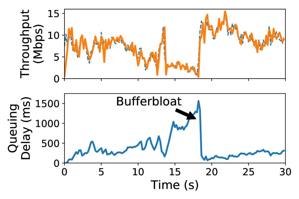
(a) Cubic

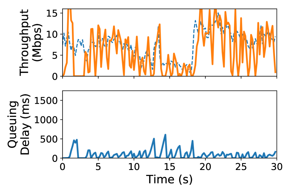
(b) Verus

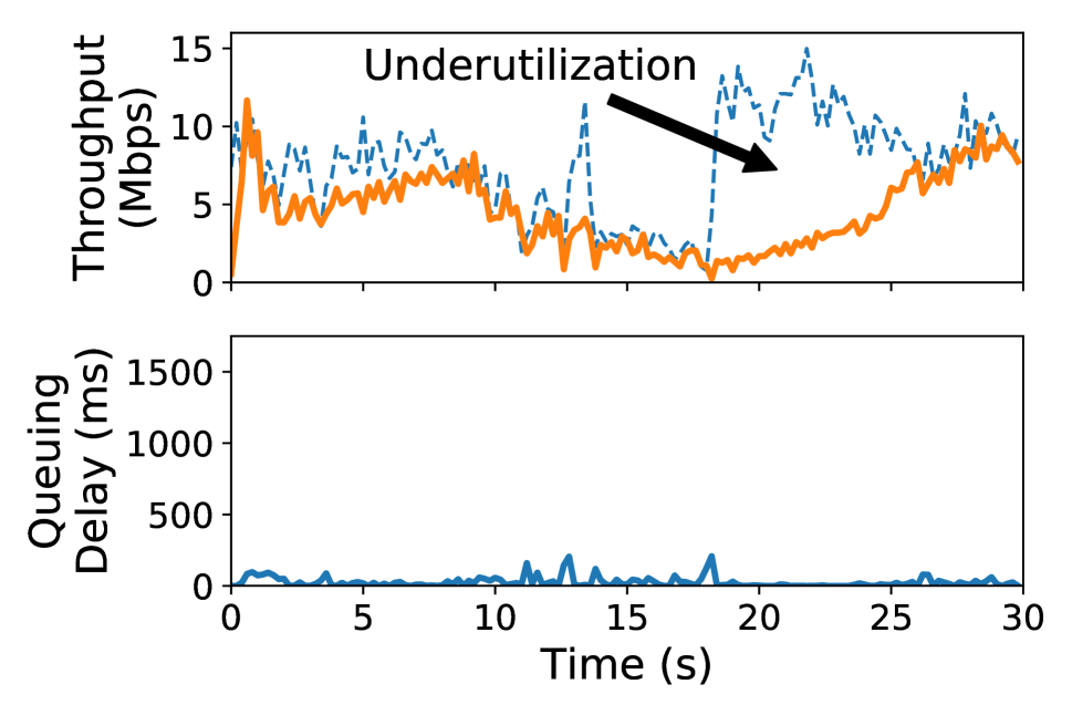
(c) Cubic+CoDel

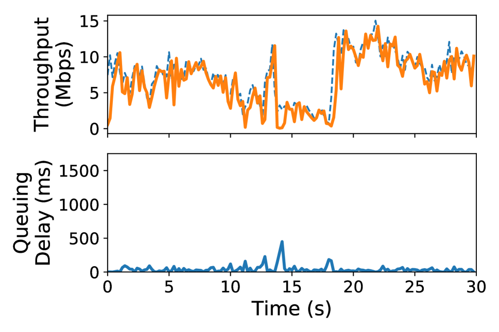
(d) ABC

Figure 1: Performance on a emulated cellular trace — The dashed blue in the top graph represents link capacity, the solid orange line represents the achieved throughput. Cubic has high utilization but has very high delays (up to 1500 milliseconds). Verus has large rate variations and incurs high delays. Cubic+CoDel reduces queuing delays significantly, but leaves the link underutilized when capacity increases. ABC achieves close to 100% utilization while maintaining low queuing delays (similar to that of Cubic+CoDel).

Limitations of end-to-end congestion control: Traditional end-to-end congestion control schemes like Cubic [23] and NewReno [24] rely on packet drops to infer congestion and adjust their rates. Such schemes tend to fill up the buffer, causing large queuing delays, especially in cellular networks that use deep buffers to avoid packet loss [47]. Fig. 1(a) shows performance of Cubic on an LTE link, emulated using a LTE trace with Mahimahi [36]. The network round-trip time is 100 ms and the buffer size is set to 250 packets. Cubic causes significant queuing delay, particularly when the link capacity drops.

Recent proposals such as BBR [14], PCC-Vivace [16] and Copa [10] use RTT and send/receive rate measurements to estimate the available link rate more accurately. Although these schemes are an improvement over loss-based schemes, their performance is far from optimal on highly-variable links. Our experiments show that they either cause excessive queuing or underutilize the link capacity (e.g., see Fig. 7). Sprout [47] and Verus [51] are two other recent end-to-end protocols designed specifically for cellular networks. They also have difficulty tracking the link rate accurately; depending on parameter settings, they can be too aggressive (causing large queues) or too conservative (hurting utilization). For example, Fig. 1(b) shows how Verus performs on the same LTE trace as above.

The fundamental challenge for any end-to-end scheme is that to estimate the link capacity, it must utilize the link fully and build up a queue. When the queue is empty, signals such as the RTT and send/receive rate do not provide information about the available capacity. Therefore, in such periods, all end-to-end schemes must resort to some form of “blind” rate increase. But for networks with a large dynamic range of rates, it is very difficult to tune this rate increase correctly: if it is slow, throughput suffers, but making it too fast causes overshoots and large queuing delays. For schemes that attempt to limit queue buildup, periods in which queues go empty (and a blind rate increase is necessary) are common; they occur, for example, following a sharp increase in link capacity.

AQM schemes do not signal increases: AQM schemes like RED [19], PIE [38] and CoDel [2] can be used to signal congestion (via ECN or drops) before the buffer fills up at the bottleneck link, reducing delays. However, AQM schemes do not signal rate increases. When capacity increases, the sender must again resort to a blind rate increase. Fig. 1(c) shows how CoDel performs when the sender is using Cubic. Cubic+CoDel reduces delays by 1 to 2 orders of magnitude compared to Cubic alone but leaves the link underutilized when capacity increases.

Thus, we conclude that, both end-to-end and AQM-based schemes will find it difficult to track time-varying wireless link rates accurately. Explicit control schemes, such as XCP [29] and RCP [44] provide a compelling alternative. The router provides multiple bits of feedback per packet to senders based on direct knowledge of the wireless link capacity. By telling senders precisely how to increase or decrease their rates, explicit schemes can quickly adapt to time-varying links, in principle, within an RTT of link capacity changes.

Deployment challenges for explicit congestion control: Schemes like XCP and RCP require major changes to packet headers, routers, and endpoints. Although the changes are technically feasible, in practice, they create significant deployment challenges. For instance, these protocols require new packet fields to carry multi-bit feedback information. IP or TCP options could in principle be used for these fields. But many wide-area routers drop packets with IP options [20], and using TCP options creates problems due to middleboxes [25] and IPSec encryption [30]. Another important challenge is co-existence with legacy routers and legacy transport protocols. To be deployable, an explicit protocol must handle scenarios where the bottleneck is at a legacy router, or when it shares the link with standard end-to-end protocols like Cubic.

Design goals: In designing ABC, we targeted the following properties:

1. Control algorithm for fast-varying wireless links: Prior explicit control algorithms like XCP and RCP were designed for fixed-capacity links. We design ABC’s control algorithm specifically to handle the rapid bandwidth variations and packet transmission behavior of wireless links (e.g., frame batching at the MAC layer).

2. No modifications to packet headers: ABC repurposes the existing ECN [42] bits to signal both increases and decreases to the sender’s congestion window. By spreading feedback over a sequence of 1-bit signals per packet, ABC routers precisely control sender congestion windows over a large dynamic range.

3. Coexistence with legacy bottleneck routers: ABC is robust to scenarios where the bottleneck link is not the wireless link but a non-ABC link elsewhere on the path. Whenever a non-ABC router becomes the bottleneck, ABC senders ignore window increase feedback from the wireless link, and ensure that they send no faster than their fair share of the bottleneck link.

4. Coexistence with legacy transport protocols: ABC routers ensure that ABC and non-ABC flows share a wireless bottleneck link fairly. To this end, ABC routers separate ABC and non-ABC flows into two queues, and use a simple algorithm to schedule packets from these queues. ABC makes no assumptions about the congestion control algorithm of non-ABC flows, is robust to the presence of short or application-limited flows, and requires a small amount of state at the router.

Fig. 1(d) shows ABC on the same emulated LTE link. Using only one bit of feedback per packet, the ABC flow is able to track the variations in bottleneck link closely, achieving both high throughput and low queuing delay.

3 Design

ABC is a window-based protocol: the sender limits the number of packets in flight to the current congestion window. Window-based protocols react faster to the sudden onset of congestion than rate-based schemes [11]. On a wireless link, when the capacity drops and the sender stops receiving ACKs, ABC will stop sending packets immediately, avoiding further queue buildup. In contrast, a rate-based protocol would take time to reduce its rate and may queue up a large number of packets at the bottleneck link in the meantime.

ABC senders adjust their window size based on explicit feedback from ABC routers. An ABC router uses its current estimate of the link rate and the queuing delay to compute a target rate. The router then sets one bit of feedback in each packet to guide the senders towards the target rate. Each bit is echoed to a sender by a receiver in an ACK, and it signals either a one-packet increase (“accelerate”) or a one-packet decrease (“brake”) to the sender’s congestion window.

3.1 The ABC Protocol

We now present ABC’s design starting with the case where all routers are ABC-capable and all flows use ABC. We later discuss how to extend the design to handle non-ABC routers and scenarios with competing non-ABC flows.

3.1.1 ABC Sender

On receiving an “accelerate” ACK, an ABC sender increases its congestion window by 1 packet. This increase results in two packets being sent, one in response to the ACK and one due to the window increase. On receiving a “brake,” the sender reduces its congestion window by 1 packet, preventing the sender from transmitting a new packet in response to the received ACK. As we discuss in §4.3, the sender also performs an additive increase of 1 packet per RTT to achieve fairness. For ease of exposition, let us ignore this additive increase for now.

Though each bit of feedback translates to only a small change in the congestion window, when aggregated over an RTT, the feedback can express a large dynamic range of window size adjustments. For example, suppose a sender’s window size is $w$, and the router marks accelerates on a fraction $f$ of packets in that window. Over the next RTT, the sender will receive $w\cdot f$ accelerates and $w-w\cdot f$ brakes. Then, the sender’s window size one RTT later will be $w+wf-(w-wf)=2wf$ packets. Thus, in one RTT, an ABC router can vary the sender’s window size between zero ($f$ = 0) and double its current value ($f=1$). The set of achievable window changes for the next RTT depends on the number of packets in the current window $w$; the larger $w$, the higher the granularity of control.

In practice, ABC senders increase or decrease their congestion window by the number of newly acknowledged bytes covered by each ACK. Byte-based congestion window modification is a standard technique in many TCP implementations [8], and it makes ABC robust to variable packet sizes and delayed, lost, and partial ACKs. For simplicity, we describe the design with packet-based window modifications in this paper.

3.1.2 ABC Router

Calculating the target rate: ABC routers compute the target rate $tr(t)$ using the following rule:

$$tr(t)=\eta{\mu(t)}-\frac{\mu(t)}{\delta}(x(t)-d_{t})^{+},\vspace{-3mm}$$ (1)

where $\mu(t)$ is the link capacity, $x(t)$ is the observed queuing delay, $d_{t}$ is a pre-configured delay threshold, $\eta$ is a constant less than 1, $\delta$ is a positive constant (in units of time), and $y^{+}$ is $\max(y,0)$. This rule has the following interpretation. When queuing delay is low ($x(t)<d_{t}$), ABC sets the target rate to $\eta\mu(t)$, for a value of $\eta$ slightly less than 1 (e.g., $\eta=0.95$). By setting the target rate a little lower than the link capacity, ABC aims to trade a small amount of bandwidth for large reductions in delay, similar to prior work [27, 7, 33]. However, queues can still develop due to rapidly changing link capacity and the 1 RTT of delay it takes for senders to achieve the target rate. ABC uses the second term in Equation (1) to drain queues. Whenever $x(t)>d_{t}$, this term reduces the target rate by an amount that causes the queuing delay to decrease to $d_{t}$ in at most $\delta$ seconds.

The threshold $d_{t}$ ensures that the target rate does not react to small increases in queuing delay. This is important because wireless links often schedule packets in batches. Queuing delay caused by batch packet scheduling does not imply congestion, even though it occurs persistently. To prevent target rate reductions due to this delay, $d_{t}$ must be configured to be greater than the average inter-scheduling time at the router.

ABC’s target rate calculation requires an estimate of the underlying link capacity, $\mu(t)$. In $\S$5, we discuss how to estimate the link capacity in cellular and WiFi networks, and we present an implementation for WiFi.

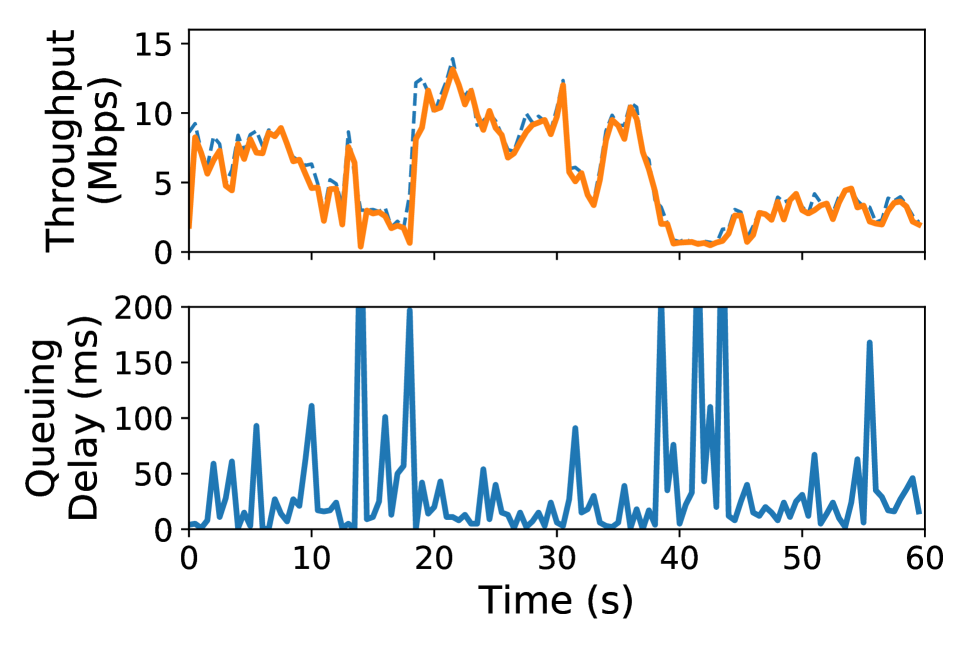
(a) Dequeue

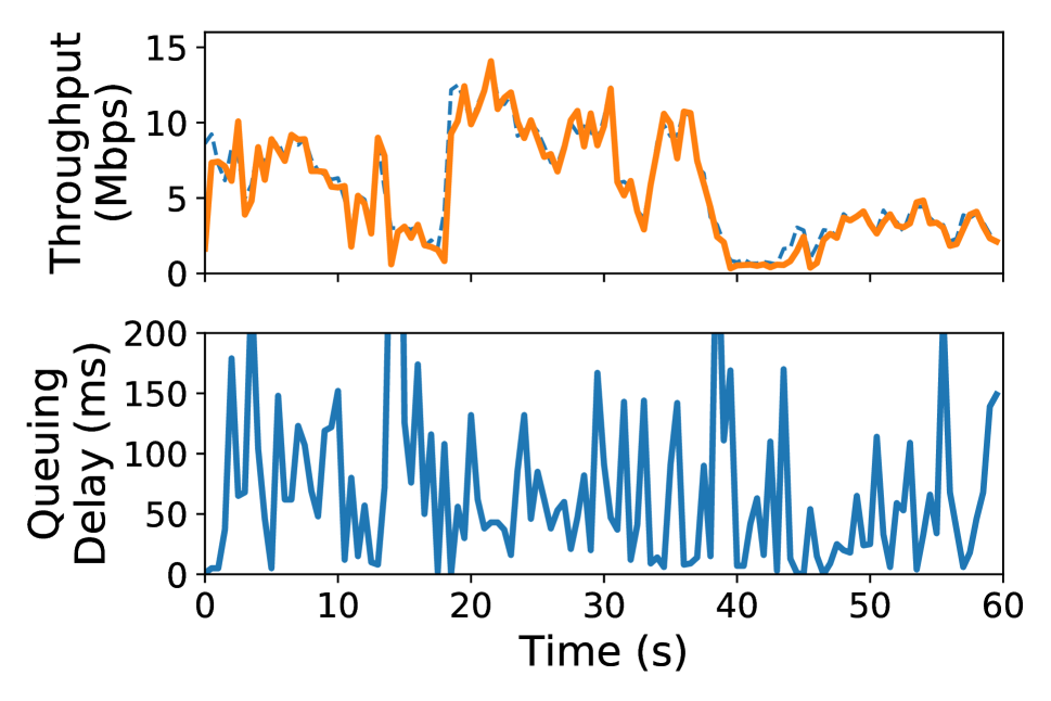
(b) Enqueue

Figure 2: Feedback — Calculating $f(t)$ based on enqueue rate increases $95^{th}$ percentile queuing delay by 2$\times$.

Packet marking: To achieve a target rate, $tr(t)$, the router computes the fraction of packets, $f(t)$, that should be marked as accelerate. Assume that the current dequeue rate — the rate at which the router transmits packets — is $cr(t)$. If the accelerate fraction is $f(t)$, for each packet that is ACKed, the sender transmits $2f(t)$ packets on average. Therefore, after 1 RTT, the enqueue rate — the rate at which packets arrive to the router — will be $2cr(t)f(t)$. To achieve the target rate, $f(t)$ must be chosen such that $2cr(t)f(t)$ is equal to $tr(t)$. Thus, $f(t)$ is given by:

$$\vspace{-2mm}f(t)=\min\Big{\{}\frac{1}{2}\cdot\frac{tr(t)}{cr(t)},1\Big{\}}.$$ (2)

An important consequence of the above calculation is that $f(t)$ is computed based on the dequeue rate. Most explicit protocols compare the enqueue rate to the link capacity to determine the feedback (e.g., see XCP [29]).

ABC uses the dequeue rate instead to exploit the ACK-clocking property of its window-based protocol. Specifically, Equation (2) accounts for the fact that when the link capacity changes (and hence the dequeue rate changes), the rate at the senders changes automatically within 1 RTT because of ACK clocking. Fig. 2 demonstrates that computing $f(t)$ based on the dequeue rate at the router enables ABC to track the link capacity much more accurately than using the enqueue rate.

ABC recomputes $f(t)$ on every dequeued packet, using measurements of $cr(t)$ and $\mu(t)$ over a sliding time window of length $T$. Updating the feedback on every packet allows ABC to react to link capacity changes more quickly than schemes that use periodic feedback updates (e.g., XCP and RCP).

Packet marking can be done deterministically or probabilistically. To limit burstiness, ABC uses the deterministic method in Algorithm 1. The variable token implements a token bucket that is incremented by $f(t)$ on each outgoing packet (up to a maximum value tokenLimit), and decremented when a packet is marked accelerate. To mark a packet accelerate, token must exceed 1. This simple method ensures that no more than a fraction $f(t)$ of the packets are marked accelerate.

 token $=$ 0;

for each outgoing packet do

       calculate $f(t)$ using Equation (2);

       token = min(token $+f(t)$, tokenLimit);

       if packet marked with accelerate then

             if token $>$ 1 then

                   token = token $-$ 1;

                   mark accelerate;

                  

            else

                   mark brake;

                  

Algorithm 1 Packet marking at an ABC router.

Multiple bottlenecks: An ABC flow may encounter multiple ABC routers on its path. An example of such a scenario is when two smartphone users communicate over an ABC-compliant cellular network. Traffic sent from one user to the other will traverse a cellular uplink and cellular downlink, both of which could be the bottleneck. To support such situations, an ABC sender should send traffic at the smallest of the router-computed target rates along their path. To achieve this goal, each packet is initially marked accelerate by the sender. ABC routers may change a packet marked accelerate to a brake, but not vice versa (see Algorithm 1). This rule guarantees that an ABC router can unilaterally reduce the fraction of packets marked accelerate to ensure that its target rate is not exceeded, but it cannot increase this fraction. Hence the fraction of packets marked accelerate will equal the minimum $f(t)$ along the path.

3.1.3 Fairness

Multiple ABC flows sharing the same bottleneck link should be able to compete fairly with one another. However, the basic window update rule described in  $\S$3.1.1 is a multiplicative-increase/multiplicative-decrease (MIMD) strategy, which does not provide fairness among contending flows (see Fig. 3(a) for an illustration). To achieve fairness, we add an additive-increase (AI) component to the basic window update rule. Specifically, ABC senders adjust their congestion window on each ACK as follows:

$$w\leftarrow\begin{cases}w+1+1/w&\text{if accelerate}\\ w-1+1/w&\text{if brake}\end{cases}\vspace{-1mm}$$ (3)

This rule increases the congestion window by 1 packet each RTT, in addition to reacting to received accelerate and brake ACKs. This additive increase, coupled with ABC’s MIMD response, makes ABC a multiplicative-and-additive-increase/multiplicative-decrease (MAIMD) scheme. Chiu and Jain [15] proved that MAIMD schemes converge to fairness (see also [5]). Fig. 3(b) shows how with an AI component, competing ABC flows achieve fairness.

To give intuition, we provide a simple informal argument for why including additive increase gives ABC fairness. Consider $N$ ABC flows sharing a link, and suppose that in steady state, the router marks a fraction $f$ of the packets accelerate, and the window size of flow $i$ is $w_{i}$. To be in steady state, each flow must send 1 packet on average for each ACK that it receives. Now consider flow $i$. It will send $2f+1/w_{i}$ packets on average for each ACK: $2f$ for the two packets it sends on an accelerate (with probability $f$), and $1/w_{i}$ for the extra packet it sends every $w_{i}$ ACKs. Therefore, to be in steady state, we must have: $2f+1/w_{i}=1\implies w_{i}=1/(1-2f)$. This shows that the steady-state window size for all flows must be the same, since they all observe the same fraction $f$ of accelerates. Hence, with equal RTTs, the flows will have the same throughput, and otherwise their throughput will be inversely proportional to their RTT. Note that the RTT unfairness in ABC is similar to that of schemes like Cubic, for which the throughput of a flow is inversely proportional to its RTT. In  $\S$7.5, we show experiments where flows have different RTTs.

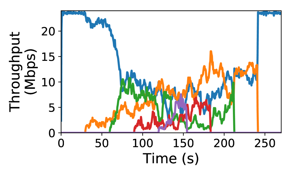
(a) ABC w/o AI

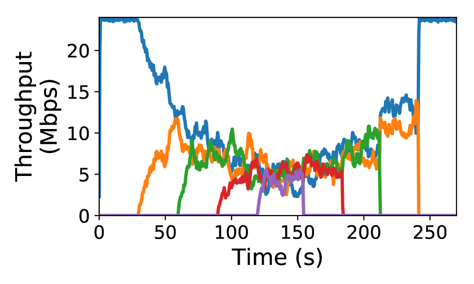
(b) ABC with AI

Figure 3: Fairness among competing ABC flows — 5 flows with the same RTT start and depart one-by-one on a 24 Mbit/s link. The additive-increase (AI) component leads to fairness.

3.1.4 Stability Analysis

ABC’s stability depends on the values of $\eta$ and $\delta$. $\eta$ determines the target link utilization, while $\delta$ controls how long it will take for a queue to drain. In Appendix C, we prove the following result for a fluid model of the ABC control loop.

Theorem 1.

Consider a single ABC link, traversed by $N$ ABC flows. Let $\tau$ be the maximum round-trip propagation delay of the flows. ABC is globally asymptotically stable if

$$\delta>\frac{2}{3}\cdot\tau.\vspace{-8mm}$$ (4)

Specifically, if $\mu(t)=\mu$ for $t>t_{0}$ (i.e., the link capacity stops changing after some time $t_{0}$), the enqueue/dequeue rate and the queuing delay at the ABC router will converge to certain values $r^{*}$ and $x^{*}$ that depend on the system parameters and the number of flows. In all cases: $\eta\mu<r^{*}\leq\mu$.

This stability criterion is simple and intuitive. It states that $\delta$ should not be much smaller than the RTT (i.e, the feedback delay). If $\delta$ is very small, ABC reacts too forcefully to queue build up, causing under-utilization and oscillations. Increasing $\delta$ well beyond $2/3\tau$ improves the stability margins of the feedback loop, but hurts responsiveness. In our experiments, we used $\delta=133$ ms for a propagation RTT of $100$ ms.

4 Coexistence

An ABC flow should be robust to presence of non-ABC bottlenecks on its path and share resources fairly with non-ABC flows sharing the ABC router.

4.1 Deployment with non-ABC Routers

An ABC flow can encounter both ABC and non-ABC routers on its path. For example, a Wi-Fi user’s traffic may traverse both a Wi-Fi router (running ABC) and an ISP router (not running ABC); either router could be the bottleneck at any given time. ABC flows must therefore be able to detect and react to traditional congestion signals—both drops and ECN—and they must determine when to ignore accelerate feedback from ABC routers because the bottleneck is at a non-ABC router.

We augment the ABC sender to maintain two congestion windows, one for tracking the available rate on ABC routers ($w_{\mbox{abc}}$), and one for tracking the rate on non-ABC bottlenecks ($w_{\mbox{nonabc}}$). $w_{\mbox{abc}}$ obeys accelerates/brakes using Equation (3), while $w_{\mbox{nonabc}}$ follows a rule such as Cubic [23] and responds to drop and ECN signals. An ABC sender must send packets to match the lower of the two windows. Our implementation mimics Cubic for the non-ABC method, but other methods could also be emulated.

With this approach, the window that is not the bottleneck could become large. For example, when a non-ABC router is the bottleneck, the ABC router will continually send accelerate signals, causing $w_{\mbox{abc}}$ to grow. If the ABC router later becomes the bottleneck, it will temporarily incur large queues. To prevent this problem, ABC senders cap both $w_{\mbox{abc}}$ and $w_{\mbox{nonabc}}$ to $2\times$ the number of in-flight packets.

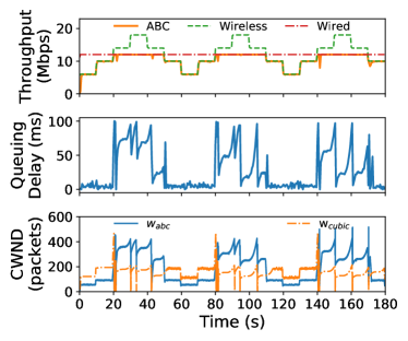
Figure 4: Coexistence with non-ABC bottlenecks — When the wired link is the bottleneck, ABC becomes limited by $w_{\mbox{cubic}}$ and behaves like a Cubic flow. When the wireless link is the bottleneck, ABC uses $w_{abc}$ to achieve low delays and high utilization.

Fig. 4 shows the throughput and queuing delay for an ABC flow traversing a path with an ABC-capable wireless link and a wired link with a droptail queue. For illustration, we vary the rate of the wireless link in a series of steps every 5 seconds. Over the experiment, the bottleneck switches between the wired and wireless links several times. ABC is able to adapt its behavior quickly and accurately. Depending on which link is the bottleneck, either $w_{\mbox{nonabc}}$ (i.e., $w_{\mbox{cubic}}$) or $w_{\mbox{abc}}$ becomes smaller and controls the rate of the flow. When the wireless link is the bottleneck, ABC maintains low queuing delay, whereas the queuing delay exhibits standard Cubic behavior when the wired link is the bottleneck. $w_{\mbox{cubic}}$ does not limit ABC’s ability to increase its rate when the wireless link is the bottleneck. At these times (e.g., around the 70 s mark), as soon on $w_{\mbox{abc}}$ increases, the number of in-flight packets and the cap on $w_{\mbox{cubic}}$ increases, and $w_{\mbox{cubic}}$ rises immediately.

4.2 Multiplexing with ECN Bits

IP packets have two ECN-related bits: ECT and CE. These two bits are traditionally interpreted as follows:

ECT	CE	Interpretation
0	0	Non-ECN-Capable Transport
0	1	ECN-Capable Transport ECT(1)
1	0	ECN-Capable Transport ECT(0)
1	1	ECN set

Routers interpret both 01 and 10 to indicate that a flow is ECN-capable, and routers change those bits to 11 to mark a packet with ECN. Upon receiving an ECN mark (11), the receiver sets the ECN Echo (ECE) flag to signal congestion to the sender. ABC reinterprets the ECT and CE bits as follows:

ECT	CE	Interpretation
0	0	Non-ECN-Capable Transport
0	1	Accelerate
1	0	Brake
1	1	ECN set

ABC send all packets with accelerate (01) set, and ABC routers signal brakes by flipping the bits to 10. Both 01 and 10 indicate an ECN-capable transport to ECN-capable legacy routers, which will continue to use (11) to signal congestion.

With this design, receivers must be able to echo both standard ECN signals and accelerates/brakes for ABC. Traditional ECN feedback is signaled using the ECE flag. For ABC feedback, we repurpose the NS (nonce sum) bit, which was originally proposed to ensure ECN feedback integrity [17] but has been reclassified as historic [32] due to lack of deployment. Thus, it appears possible to deploy ABC with only simple modifications to TCP receivers.

Deployment in proxied networks: Cellular networks commonly split TCP connections and deploy proxies at the edge [46, 43]. Here, it is unlikely that any non-ABC router will be the bottleneck and interfere with the accel-brake markings from the ABC router. In this case, deploying ABC may not require any modifications to today’s TCP ECN receiver. ABC senders (running on the proxy) can use either 10 or 01 to signal an accelerate, and routers can use 11 to indicate a brake. The TCP receiver can echo this feedback using the ECE flag.

4.3 Non-ABC flows at an ABC Router

ABC flows are potentially at a disadvantage when they share an ABC bottleneck link with non-ABC flows. If the non-ABC flows fill up queues and increase queuing delay, the ABC router will reduce ABC’s target rate. To ensure fairness in such scenarios, ABC routers isolate ABC and non-ABC packets in separate queues.

We assume that ABC routers can determine whether a packet belongs to an ABC flow. In some deployment scenarios, this is relatively straightforward. For example, in a cellular network deployment with TCP proxies at the edge of the network [46, 43], the operator can deploy ABC at the proxy, and configure the base station to assume that all traffic from the proxy’s IP address uses ABC. Other deployment scenarios may require ABC senders to set a predefined value in a packet field like the IPv6 flow label or the IPv4 IPID.

The ABC router assigns weights to the ABC and non-ABC queues, respectively, and it schedules packets from the queues in proportion to their weights. In addition, ABC’s target rate calculation considers only ABC’s share of the link capacity (which is governed by the weights). The challenge is to set the weights to ensure that the average throughput of long-running ABC and non-ABC flows is the same, no matter how many flows there are.

Prior explicit control schemes address this problem using the TCP loss-rate equation (XCP) or by estimating the number of flows with Zombie Lists (RCP). Relying on the TCP equation requires a sufficient loss rate and does not handle flows like BBR. RCP’s approach does not handle short flows. When one queue has a large number of short flows (and hence a low average throughput), RCP increases the weight of that queue. However, the short flows cannot send faster, so the extra bandwidth is taken by long-running flows in the same queue, which get more throughput than long-running flows in the other queue (see §7.5 for experimental results).

To overcome these drawbacks, a ABC router measures the average rate of the $K$ largest flows in each queue using the Space Saving Algorithm [35], which requires $\mathcal{O}(K)$ space. It considers any remaining flow in either queue to be short, and it calculates the total rate of the short flows in each queue by subtracting the rate of the largest $K$ flows from the queue’s aggregate throughput. ABC uses these rate measurements to estimate the rate demands of the flows. Using these demands, ABC periodically computes the max-min fair rate allocation for the flows, and it sets the weight of each of the two queues to be equal to the total max-min rate allocation of its component flows. This algorithm ensures that long-running flows in the two queues achieve the same average rate, while accounting for demand-limited short flows.

To estimate the demand of the flows, the ABC router assumes that the demand for the top $K$ flows in each queue is X% higher than the current throughput of the flow, and the aggregate demand for the short flows is the same as their throughput. If a top-$K$ flow is unable to increase its sending rate by X%, its queue’s weight will be larger than needed, but any unfairness in weight assignment is bounded by X%. Small values of $X$ limit unfairness but can slow down convergence to fairness; our experiments use $X=10\%$.

5 Estimating Link Rate

We describe how ABC routers can estimate the link capacity for computing the target rate (§3.1.2). We present a technique for Wi-Fi that leverages the inner workings of the Wi-Fi MAC layer, and we discuss options for cellular networks.

5.1 Wi-Fi

We describe how an 802.11n access point (AP) can estimate the average link rate. For simplicity, we first describe our solution when there is a single user (client) connected to the AP. Next, we describe the multi-user case.

We define link rate as the potential throughput of the user (i.e., the MAC address of the Wi-Fi client) if it was backlogged at the AP, i.e., if the user never ran out of packets at the AP. In case the router queue goes empty at the AP, the achieved throughput will be less than the link rate.

Challenges: A strawman would be to estimate the link rate using the physical layer bit rate selected for each transmission, which would depend on the modulation and channel code used for the transmission. Unfortunately, this method will overestimate the link rate as the packet transmission times are governed not only by the bitrate, but also by delays for additional tasks (e.g., channel contention and retransmissions [12]). An alternative approach would be to use the fraction of time that the router queue was backlogged as a proxy for link utilization. However, the Wi-Fi MAC’s packet batching confounds this approach. Wi-Fi routers transmit packets (frames) in batches; a new batch is transmitted only after receiving an ACK for the last batch. The AP may accumulate packets while waiting for a link-layer ACK; this queue buildup does not necessarily imply that the link is fully utilized. Thus, accurately measuring the link rate requires a detailed consideration of Wi-Fi’s packet transmission protocols.

Understanding batching: In 802.11n, data frames, also known as MAC Protocol Data Units (MPDUs), are transmitted in batches called A-MPDUs (Aggregated MPDUs). The maximum number of frames that can be included in a single batch, $M$, is negotiated by the receiver and the router. When the user is not backlogged, the router might not have enough data to send a full-sized batch of $M$ frames, but will instead use a smaller batch of size $b<M$. Upon receiving a batch, the receiver responds with a single Block ACK. Thus, at a time $t$, given a batch size of $b$ frames, a frame size of $S$ bits, and an ACK inter-arrival time (i.e., the time between receptions of consecutive block ACKs) of $T_{IA}(b,t)$, the current dequeue rate, $cr(t)$, may be estimated as

$$cr(t)=\frac{b\cdot S}{T_{IA}(b,t)}.$$ (5)

When the user is backlogged and $b=M$, then $cr(t)$ above will be equal to the link capacity. However, if the user is not backlogged and $b<M$, how can the AP estimate the link capacity? Our approach calculates $\hat{T}_{IA}(M,t)$, the estimated ACK inter-arrival time if the user was backlogged and had sent $M$ frames in the last batch.

We estimate the link capacity, $\hat{\mu}(t)$, as

$$\hat{\mu}(t)=\frac{M\cdot S}{\hat{T}_{IA}(M,t)}.$$ (6)

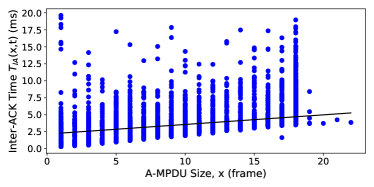
Figure 5: Inter-ACK time v. batch (A-MPDU) size — Inter-ACK times for a given batch size exhibits variation. The solid black line represents the average Inter-ACK time. The slope of the line is $S/R$, where $S$ is the frame size in bits and $R$ is the link rate in bits per second.

To accurately estimate $\hat{T}_{IA}(M,t)$, we turn to the relationship between the batch size and ACK inter-arrival time. We can decompose the ACK interval time into the batch transmission time and “overhead” time, the latter including physically receiving an ACK, contending for the shared channel, and transmitting the physical layer preamble [21]. Each of these overhead components is independent of the batch size. We denote the overhead time by $h(t)$. If $R$ is the bitrate used for transmission, the router’s ACK inter-arrival time is

$$T_{IA}(b,t)\; =\;\frac{b\cdot S}{R}+h(t).$$ (7)

Fig. 5 illustrates this relationship empirically. There are two key properties to note. First, for a given batch size, the ACK inter-arrival times vary due to overhead tasks. Second, because the overhead time and batch size are independent, connecting the average values of ACK inter-arrival times across all considered batch sizes will produce a line with slope $S/R$. Using this property along with Equation (7), we can estimate the ACK inter-arrival time for a backlogged user as

$$\hat{T_{IA}}(M,t)\; =\;\frac{M\cdot S}{R}+h(t)$$

$$=\;T_{IA}(b,t)+\frac{(M-b)\cdot S}{R}\cdot$$ (8)

We can then use $\hat{T}_{IA}(M,t)$ to estimate the link capacity with Equation (6). This computation is performed for each batch transmission when the batch ACK arrives, and passed through a weighted moving average filter over a sliding window of time $T$ to estimate the smoothed time-varying link rate. $T$ must be greater than the inter-ACK time (up to 20 ms in Fig. 5); we use $T=40$ ms. Because ABC cannot exceed a rate-doubling per RTT, we cap the predicted link rate to double the current rate (dashed slanted line in Fig. 5).

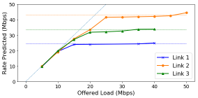
Figure 6: Wi-Fi Link Rate Prediction — ABC router link rate predictions for a user that was not backlogged and sent traffic at multiple different rates over three different Wi-Fi links. Horizontal lines represent the true link capacity, solid lines summarize the ABC router’s link capacity prediction (each point is an average over 30 seconds of predictions), and the dashed slanted line represents the prediction rate caps. ABC’s link rate predictions are within 5% of the ground truth across most sending rates (given the prediction cap).

To evaluate the accuracy of our link rate estimates, we transmit data to a single client through our modified ABC router ($\S$7.1) at multiple different rates over three Wi-Fi links (with different modulation and coding schemes). Fig. 6 summarizes the accuracy of the ABC router’s link rate estimates. With this method, the ABC Wi-Fi router is able to predict link rates within 5% of the true link capacities.

Extension to multiple users. In multi-user scenarios, each receiver will negotiate its own maximum batch size ($M$) with the router, and different users can have different transmission rates. We now present two variants of our technique for (1) when the router uses per-user queues to schedule packets of different users, and (2) when the users share a single FIFO (first-in first-out) queue at the router.

Per-user queues. In this case each user calculates a separate link rate estimate. Recall that the link rate for a given user is defined as the potential throughput of the user if it was backlogged at the router. To determine the link rate for a user $x$, we repeat the single-user method for the packets and queue of user $x$ alone, treating transmissions from other users as overhead time. Specifically, user $x$ uses Equations (8) and (6) to compute its link rate ($\hat{\mu}_{x}(t)$) based on its own values of the bit rate ($R_{x}$) and maximum batch size ($M_{x}$). It also computes its current dequeue rate ($cr_{x}(t)$) using Equation (5) to calculate the accel-brake feedback. The inter-ACK time ($T_{IA_{x}}(b,t)$), is defined as the time between the reception of consecutive block-ACKs for user $x$. Thus, the overhead time ($h_{x}(t)$) includes the time when other users at the same AP are scheduled to send packets. Fairness among different users is ensured via scheduling users out of separate queues.

Single queue. In this case the router calculates a single aggregate link rate estimate. The inter-ACK time here is the time between two consecutive block-ACKs, regardless of the user to which the block-ACKs belong to. The router tries to match the aggregate rate of the senders to the aggregate link rate, and uses the aggregate current dequeue rate to calculate accel-brake feedback.

5.2 Cellular Networks

Cellular networks schedule users from separate queues to ensure inter-user fairness. Each user will observe a different link rate and queuing delay. As a result, every user requires a separate target rate calculation at the ABC router. The 3GPP cellular standard [1] describes how scheduling information at the cellular base station can be used to calculate per-user link rates. This method is able to estimate capacity even if a given user is not backlogged at the base station, a key property for the target rate estimation in Equation (1).

6 Discussion

We discuss practical issues pertaining to ABC’s deployment.

Delayed Acks: To support delayed ACKs, ABC uses byte counting at the sender; the sender increases/decreases its window by the new bytes ACKed. At the receiver, ABC uses the state machine from DCTCP [6] for generating ACKs and echoing accel/brake marks. The receiver maintains the state of the last packet (accel or brake). Whenever the state changes, the receiver sends an ACK with the new state. If the receiver is in the same state after receiving $m$ packets (the number of ACKs to coalesce), then it sends a delayed ACK with the current state. Our TCP implementation and the experiments in $\S$7 use delayed ACKs with $m=2$.

Lost ACKs: ABC’s window adjustment is robust to ACK losses. Consider a situation where the sender receives a fraction $p<1$ of the ACKs. If the accelerate fraction at the router is $f$, the current window of the sender is $w_{abc}$, then in the next RTT, the change in congestion window of the sender is $fpw_{abc}-(1-f)pw_{abc}=(2f-1)pw_{abc}$. As a result, lost ACKs only slow down the changes in the congestion window, but whether it increases or decreases doesn’t depend on $p$.

ABC routers don’t change prior ECN marks: ABC routers don’t mark accel-brake on incoming packets that contain ECN marks set by an upstream non-ABC router. Since packets with ECN set can’t convey accel-brake marks, they can slow down changes in $w_{abc}$ (similar to lost ACKs). In case the fraction of packets with ECN set is small, then, the slow down in changes to $w_{abc}$ will be small. If the fraction is large, then the non-ABC router is the likely bottleneck, and the sender will not use $w_{abc}$.

ECN routers clobbering ABC marks: An ECN router can overwrite accel-brake marks. The ABC sender will still track the non-ABC window, $w_{nonabc}$, but such marks can slow down adjustment to the ABC window, $w_{abc}$.

ABC on fixed-rate links: ABC can also be deployed on fixed-rate links. On such links, its performance is similar to prior explicit schemes like XCP.

7 Evaluation

We evaluate ABC by considering the following properties:

1. Performance: We measure ABC’s ability to achieve low delay and high throughput and compare ABC to end-to-end schemes, AQM schemes, and explicit control schemes (§7.3).

2. Multiple Bottlenecks: We test ABC in scenarios with multiple ABC bottlenecks and mixtures of ABC and non-ABC bottlenecks (§7.4).

3. Fairness: We evaluate ABC’s fairness while competing against other ABC and non-ABC flows (§7.5).

4. Additional Considerations: We evaluate how ABC performs with application-limited flows and different network delays. We also demonstrate ABC’s impact on a real application’s performance (§7.6).

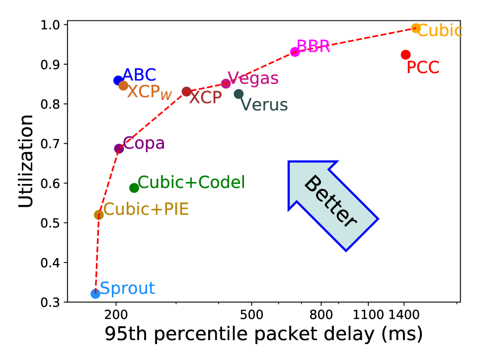
(a) Downlink

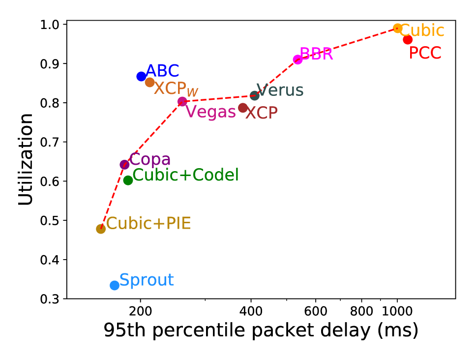
(b) Uplink

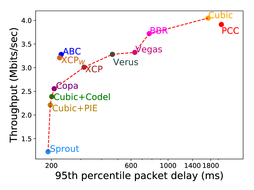
(c) Uplink+Downlink

Figure 7: ABC vs. previous schemes on three Verizon cellular network traces — In each case, ABC outperforms all other schemes and sits well outside the Pareto frontier of previous schemes (denoted by the dashed lines).

7.1 Prototype ABC Implementation

ABC transport: We implemented ABC endpoints in Linux as kernel modules using the pluggable TCP API.

ABC router: We implemented ABC as a Linux queuing discipline (qdisc) kernel module using OpenWrt, an open source operating system for embedded networked devices [18]. We used a NETGEAR WNDR 3800 router configured to 802.11n. We note that our implementation is portable as OpenWrt is supported on many other commodity Wi-Fi routers.

ABC’s WiFi link rate estimation exploits the inner workings of the MAC 802.11n protocol, and thus requires fine-grained values at this layer. In particular, the ABC qdisc must know A-MPDU sizes, Block ACK receive times, and packet transmission bitrates. These values are not natively exposed to Linux router qdiscs, and instead are only available at the network driver. To bridge this gap, we modified the router to log the relevant MAC layer data in the cross-layer socket buffer data structure (skb) that it already maintains per packet.

7.2 Experimental Setup

We evaluated ABC in both Wi-Fi and cellular network settings. For Wi-Fi, experiments we used a live Wi-Fi network and the ABC router described in $\S$7.1. For cellular settings, we use Mahimahi [36] to emulate multiple cellular networks (Verizon LTE, AT&T, and TMobile). Mahimahi’s emulation uses packet delivery traces (separate for uplink and downlink) that were captured directly on those networks, and thus include outages (highlighting ABC’s ability to handle ACK losses).

We compare ABC to end-to-end protocols designed for cellular networks (Sprout [47] and Verus [51]), loss-based end-to-end protocols both with and without AQM (Cubic [23], Cubic+Codel [37], and Cubic+PIE [38]), recently-proposed end-to-end protocols (BBR [14], Copa [10], PCC Vivace-Latency (referred as PCC)) [16]), and TCP Vegas [13]), and explicit control protocols (XCP [29], RCP [44] and VCP [48]). We used TCP kernel modules for ABC, BBR, Cubic, PCC, and Vegas; for these schemes, we generated traffic using iperf [45]. For the end-to-end schemes that are not implemented as TCP kernel modules (i.e., Copa, Sprout, Verus), we used the UDP implementations provided by the authors. Lastly, for the explicit control protocols (i.e., XCP, RCP, and VCP), we used our own implementations as qdiscs with Mahimahi to ensure compatibility with our emulation setup. We used Mahimahi’s support of Codel and Pie to evaluate AQM.

Our emulated cellular network experiments used a minimum RTT of 100 ms and a buffer size of 250 MTU-sized packets. Additionally, ABC’s target rate calculation (Equation (1)) used $\eta=0.98$ and $\delta=133$ ms. Our Wi-Fi implementation uses the link rate estimator from §5, while our emulated cellular network setup assumes the realistic scenario that ABC’s router has knowledge of the underlying link capacity [1].

7.3 Performance

Cellular: Fig. 7(a) and 7(b) show the utilization and 95^th percentile per packet delay that a single backlogged flow achieves using each aforementioned scheme on two Verizon LTE cellular link traces. ABC exhibits a better (i.e., higher) throughput/delay tradeoff than all prior schemes. In particular, ABC sits well outside the Pareto frontier of the existing schemes, which represents the prior schemes that achieve higher throughput or lower delay than any other prior schemes.

Further analysis of Fig. 7(a) and 7(b) reveals that Cubic+Codel, Cubic+PIE, Copa, and Sprout are all able to achieve low delays that are comparable to ABC. However, these schemes heavily underutilize the link. The reason is that, though these schemes are able to infer and react to queue buildups in a way that reduces delays, they lack a way of quickly inferring increases in link capacity (a common occurrence on time-varying wireless links), leading to underutilization. In contrast, schemes like BBR, Cubic, and PCC are able to rapidly saturate the network (achieving high utilization), but these schemes also quickly fill buffers and thus suffer from high queuing delays. Unlike these prior schemes, ABC is able to quickly react to both increases and decreases in available link capacity, enabling high throughput and low delays.

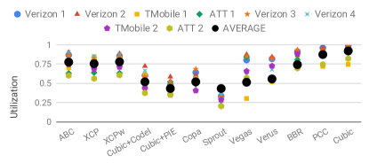
(a) Utilization

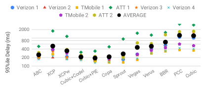
(b) $95^{th}$ percentile per-packet delay

Figure 8: 95^th percentile per-packet delay across 8 cellular link traces — On average, ABC achieves similar delays and 50% higher utilization than Copa and Cubic+Codel. PCC and Cubic achieve slightly higher throughput than ABC, but incur 380% higher 95^th percentile delay than ABC.

We observed similar trends across a larger set of 8 different cellular network traces (Fig. 8). ABC achieves 50% higher throughput than Cubic+Codel and Copa, while only incurring 17% higher $95^{th}$ percentile packet delays. PCC and Cubic achieve slightly higher link utilization values than ABC (12%, and 18%, respectively), but incur significantly higher per-packet delays than ABC (394%, and 382%, respectively). Finally, compared to BBR, Verus, and Sprout, ABC achieves higher link utilization (4%, 39%, and 79%, respectively). BBR and Verus incur higher delays (183% and 100%, respectively) than ABC. Appendix E shows mean packet delay over the same conditions, and shows the same trends.

Comparison with Explicit Protocols: Fig. 7 and 8 also show that ABC outperforms the explicit control protocol, XCP, despite not using multi-bit per-packet feedback as XCP does. For XCP we used $\alpha=0.55$ and $\beta=0.4$, the highest permissible stable values that achieve the fastest possible link rate convergence. XCP achieves similar average throughput to ABC, but with 105% higher 95^th percentile delays. This performance discrepancy can be attributed to the fact that ABC’s control rule is better suited for the link rate variations in wireless networks. In particular, unlike ABC which updates its feedback on every packet, XCP computes aggregate feedback values ($\phi$) only once per RTT and may thus take an entire RTT to inform a sender to reduce its window. To overcome this, we also considered an improved version of XCP that recomputes aggregate feedback on each packet based on the rate and delay measurements from the past RTT; we refer to this version as XCP_w (short for XCP wireless). As shown in Fig. 7 and Fig. 8, XCP_w reduces delay compared to XCP, but still incurs 40% higher 95^th percentile delays (averaged across traces) than ABC. We also compared with two other explicit schemes, RCP and VCP, and found that ABC consistently outperformed both, achieving 20% more utilization on average. (Appendix F).

(a) Single user

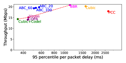
(b) Two users, shared queue

Figure 9: Throughout and mean delay on Wi-Fi — For the multi-user scenario, we report the sum of achieved throughputs and the average of observed $95^{th}$ percentile delay across both users. We consider three versions of ABC (denoted ABC _*) for different delay thresholds. All versions of ABC outperform all prior schemes and sit outside the pareto frontier.

Wi-Fi: We performed similar evaluations on a live Wi-Fi link, considering both single and multi-user scenarios. We connect senders to a WiFi router via Ethernet. Each sender transmits data through the WiFi router to one receiver. All receivers’ packets share the same FIFO queue at the router. In this experiment, we excluded Verus and Sprout as they are designed specifically for cellular networks. To mimic common Wi-Fi usage scenarios where endpoints can move and create variations in signal-to-noise ratios (and thus bitrates), we varied the Wi-Fi router’s bitrate selections by varying the MCS index using the Linux iw utility; we alternated the MCS index between values of 1 and 7 every 2 seconds. In Appendix 16, we also list results for an experiment where we model MCS index variations as Brownian motion—results show the same trends as described below. This experiment was performed in a crowded computer lab with contention from other Wi-Fi networks. We report average performance values across three, 45 second runs. We considered three different ABC delay threshold ($d_{t}$) values of 20 ms, 60 ms, and 100 ms; note that increasing ABC’s delay threshold will increase both observed throughput and RTT values.

Fig. 9 shows the throughput and $95^{th}$ percentile per-packet delay for each protocol. For the multi-user scenario, we report the sum of achieved throughputs and the average $95^{th}$ percentile delay across all users. In both the single and multi-user scenarios, ABC achieves a better throughput/delay tradeoff than all prior schemes, and falls well outside the Pareto frontier for those schemes. In the single user scenario, the ABC configuration with $d_{t}=100$ ms achieves up to 29% higher throughput than Cubic+Codel, Copa and Vegas. Though PCC-Vivace, Cubic and BBR achieve slightly higher throughput (4%) than this ABC configuration, their delay values are considerably higher (67%-6$\times$). The multi-user scenario showed similar results. For instance, ABC achieves 38%, 41% and 31% higher average throughput than Cubic+Codel, Copa and Vegas, respectively.

7.4 Coexistence with Various Bottlenecks

Coexistence with ABC bottlenecks: Fig. 7(c) compares ABC and prior protocols on a network path with two cellular links. In this scenario, ABC tracks the bottleneck link rate and achieves a better throughput/delay tradeoff than prior schemes, and again sits well outside the Pareto frontier.

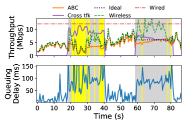
Figure 10: Coexistence with non-ABC bottlenecks — ABC tracks the ideal rate closely (fair share) and reduces queuing delays in the absence of cross traffic (white region).

Coexistence with non-ABC bottlenecks: Fig. 10 illustrates throughput and queuing delay values for an ABC flow traversing a network path with both an emulated wireless link and an emulated 12 Mbits/s fixed rate (wired) link. The wireless link runs ABC, while the wired link operates a droptail buffer. ABC shares the wired link with on-off cubic cross traffic. In the absence of cross traffic (white region), the wireless link is always the bottleneck. However, with cross traffic (yellow and grey regions), due to contention, the wired link can become the bottleneck. In this case, ABC’s fair share on the wired link is half of the link’s capacity (i.e., 6 Mbit/s). If the wireless link rate is lower than the fair share on the wired link (yellow region), the wireless link remains the bottleneck; otherwise, the wired link becomes the bottleneck (grey region).

The black dashed line in the top graph represents the ideal fair throughput for the ABC flow throughout the experiment. As shown, in all regions, ABC is able to track the ideal rate closely, even as the bottleneck shifts. In the absence of cross traffic, ABC achieves low delays while maintaining high link utilization. With cross traffic, ABC appropriately tracks the wireless link rate (yellow region) or achieves its fair share of the wired link (grey region) like Cubic. In the former cross traffic scenario, increased queuing delays are due to congestion caused by the Cubic flow on the wired link. Further, deviations from the ideal rate in the latter cross traffic scenario can be attributed to the fact that the ABC flow is running as Cubic, which in itself takes time to converge to the fair share  [23].

7.5 Fairness among ABC and non-ABC flows

Coexistence among ABC flows: We simultaneously run multiple ABC flows on a fixed 24 Mbits/s link. We varied the number of competing flows from 2 to 32 (each run was 60 s). In each case, the Jain Fairness Index [28] was within 5% from the ideal fairness value of 1, highlighting ABC’s ability to ensure fairness.

Fig. 11 shows the aggregate utilization and delay for concurrent flows (all flows running the same scheme) competing on a Verizon cellular link. We varied the number of competing flows from 1 to 16. ABC achieves similar aggregate utilization and delay across all scenarios, and, outperforms all other schemes. For all the schemes, the utilization and delay increase when the number of flows increases. For ABC, this increase can be attributed to the additional packets that result from additive increase (1 packet per RTT per flow). For other schemes, this increase is because multiple flows in aggregate ramp-up their rates faster than a single flow.

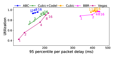
Figure 11: Coexistence among ABC flows — ABC achieves similar aggregate utilization and delay irrespective of the number of connections. ABC outperforms all previous schemes.

RTT Unfairness: We simultaneously ran 2 ABC flows on a 24 Mbits wired bottleneck. We varied the RTT of flow 1 from 20ms to 120ms. RTT of flow 2 was fixed to 20ms. Fig. 12 shows the ratio of the average throughput of these 2 flows (average throughput of flow 2 / flow 1, across 5 runs) against the ratio of their RTTs (RTT of flow 1 / flow 2). Increasing the RTT ratio increases the throughput ratio almost linearly and the throughput is inversely proportional to the RTT. Thus, the unfairness is similar to existing protocols like Cubic.

Next, we simultaneously ran 6 ABC flows. The RTT of the flows vary from 20ms to 120ms. Table 1 shows the RTT and the average throughput across 5 runs. Flows with higher RTTs have lower throughput. However, note that the flow with the highest RTT (120ms) still achieves $\sim$35 % of the throughput as flow with the lowest RTT (20ms).

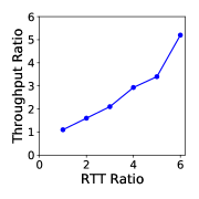
Figure 12: RTT unfairness

RTT (ms)	Tput (Mbps)
20	6.62
40	4.94
60	4.27
80	3.0
100	2.75
120	2.40

Table 1: RTT unfairness

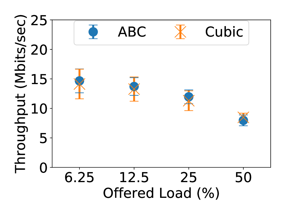
(a) ABC

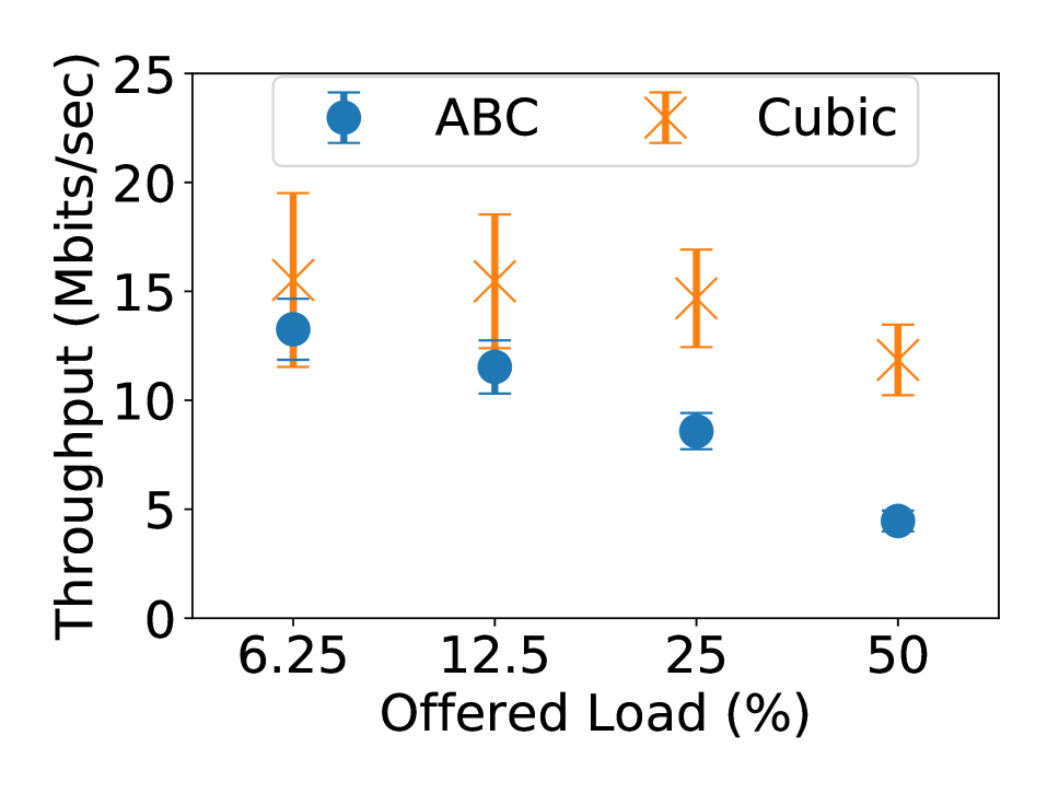
(b) RCP’s Zombie List

Figure 13: Coexistence with non-ABC flows — Across all scenarios, the standard deviation for ABC flows is small and the flows are fair to each other. Compared to RCP’s Zombie List strategy, ABC’s max-min allocation provides better fairness between ABC and non-ABC flows. With ABC’s strategy, the difference in average throughput of ABC and Cubic flows is under 5%.

Coexistence with non-ABC flows: We consider a scenario where 3 ABC and 3 non-ABC (in this case, Cubic) long-lived flows share the same 96 Mbits/s bottleneck link. In addition, we create varying numbers of non-ABC short flows (each of size 10 KB) with Poisson flow arrival times to offer a fixed average load. We vary the offered load values, and report results across 10 runs (40 seconds each). We compare ABC’s strategy to coexist with non-ABC flows to RPC’s Zombie list approach (§4.3).

Fig. 13 shows the mean and standard deviation of throughput for long-lived ABC and Cubic flows. As shown in Fig. 13(a), ABC’s coexistence strategy allows ABC and Cubic flows to fairly share the bottleneck link across all offered load values. Specifically, the difference in average throughput between the ABC and Cubic flows is under 5%. In contrast, Fig. 13(b) shows that RCP’s coexistence strategy gives higher priority to Cubic flows. This discrepancy increases as the offered load increases, with Cubic flows achieving 17-165% higher throughput than ABC flows. The reason, as discussed in  $\S$4.3, is that long-lived Cubic flows receive higher throughput than the average throughput that RCP estimates for Cubic flows. This leads to unfairness because RCP attempts to match average throughput for each scheme.Fig. 13 also shows that the standard deviation of ABC flows is small (under 10%) across all scenarios. This implies that in each run of the experiment, the throughput for each of the three concurrent ABC flows is close to each other, implying fairness across ABC flows. Importantly, the standard deviation values for ABC are smaller than those for Cubic. Thus, ABC flows converge to fairness faster than Cubic flows do.

7.6 Additional Results

ABC’s sensitivity to network latency: Thus far, our emulation experiments have considered fixed minimum RTT values of 100 ms. To evaluate the impact that propagation delay on ABC’s performance, we repeated the experiment from Fig. 8 on the RTT values of 20 ms, 50 ms, 100 ms, and 200 ms. Across all RTTs, ABC outperforms all prior schemes, again achieving a more desirable throughput/latency trade off (see Appendix  G).

Application-limited flows: We created a single long-lived ABC flow that shared a cellular link with 200 application-limited ABC flows that send traffic at an aggregate of 1 Mbit/s. Despite the fact that the application-limited flows do not have traffic to properly respond to ABC’s feedback, the ABC flows (in aggregate) still achieve low queuing delays and high link utilization. See Appendix  G for details.

Perfect future capacity knowledge: We considered a variant of ABC, PK-ABC, which knows an entire emulated link trace in advance. This experiment reflects the possibility of resource allocation predictions at cellular base stations. Rather than using an estimate of the current link rate to compute a target rate (as ABC does), PK-ABC uses the expected link rate 1 RTT in the future. On the same setup as Fig. 7(b), PK-ABC reduces 95^th percentile per-packet-delays from 97 ms to 28 ms, compared to ABC, while achieving similar utilization ($\sim$90%).

ABC’s improvement on real applications: We evaluated ABC’s improvement for real user-facing applications on a multiplayer interactive game, Slither.io [3]. We loaded Slither.io using a Google Chrome browser which ran inside an emulated cellular link with a background backlogged flow. We considered three schemes for the backlogged flow: Cubic, Cubic+Codel, and ABC. Cubic fully utilizes the link, but adds excessive queuing delays hindering gameplay. Cubic+Codel reduces queuing delays (improving user experience in the game), but underutilizes the link. Only ABC is able to achieve both high link utilization for the backlogged flow and low queuing delays for the game. A video demo of this experiment can be viewed at https://youtu.be/Dauq-tfJmyU.

Impact of $\eta$: This parameter presents a trade-off between throughput and delay. Increasing $\eta$ increases the throughput but at the cost of additional delay (see Appendix B).

8 Related Work

Several prior works have proposed using LTE infrastructure to infer the underlying link capacity [49, 34, 26]. CQIC [34] and piStream [49] use physical layer information at the receiver to estimate link capacity. However, these approaches have several limitations that lead to inaccurate estimates. CQIC’s estimation approach considers historical resource usage (not the available physical resources) [49], while piStream’s technique relies on second-level video segment downloads and thus does not account for the short timescale variations in link rate required for per-packet congestion control. These inaccuracies stem from the opacity of the base station’s resource allocation process at the receiver. ABC circumvents these issues by accurately estimating link capacity directly at the base station.

In VCP [48], router classifies congestion as low, medium, or high, and signals the sender to either perform a multiplicative increase, additive increase, or multiplicative decrease in response. Unlike an ABC sender, which reacts to ACKs individually, VCP senders act once per RTT. This coarse-grained update limits VCP’s effectiveness on time-varying wireless paths. For instance, it can take 12 RTTs to double the window. VCP is also incompatible with ECN, making it difficult to deploy.

In BMCC [41, 40], a router uses ADPM [9] to send link load information to the receiver on ECN bits, relying on TCP options to relay the feedback from the receiver to the sender. MTG proposed modifying cellular base stations to communicate the link rate explicitly using a new TCP option [26]. Both approaches do not work with IPSec encryption [30], and such packet modifications trigger the risk of packets being dropped silently by middleboxes [25]. Moreover, unlike ABC, MTG does not ensure fairness among multiple flows for a user, while BMCC has the same problem with non-BMCC flows [40, 39].

XCP-b [4] is a variant of XCP designed for wireless links with unknown capacity. XCP-b routers use the queue size to determine the feedback. When the queue is backlogged, the XCP-b router calculates spare capacity using the change in queue size and uses the same control rule as XCP. When the queue goes to zero, XCP-b cannot estimate spare capacity, and resorts to a blind fixed additive increase. Such blind increase can cause both under-utilization and increased delays ($\S$2.)

Although several prior schemes (XCP, RCP, VCP, BMCC, XCP-b) attempt to match the current enqueue rate to the capacity, none match the future enqueue rate to the capacity, and so do not perform as well as ABC on time-varying links.

9 Conclusion

This paper presented a simple new explicit congestion control protocol for time-varying wireless links called ABC. ABC routers use a single bit to mark each packet with “accelerate” or “brake”, which causes senders to slightly increase or decrease their congestion windows. Routers use this succinct feedback to quickly guide senders towards a desired target rate. ABC outperforms the best existing explicit flow control scheme, XCP, but unlike XCP, ABC does not require modifications to packet formats or user devices, making it simpler to deploy. ABC is also incrementally deployable: ABC can operate correctly with multiple ABC and non-ABC bottlenecks, and can fairly coexist with ABC and non-ABC traffic sharing the same bottleneck link. We evaluated ABC using a WiFi router implementation and trace-driven emulation of cellular links. ABC achieves 30-40% higher throughput than Cubic+Codel for similar delays, and 2.2$\times$ lower delays than BBR on a Wi-Fi path. On cellular network paths, ABC achieves 50% higher throughput than Cubic+Codel.

Acknowledgments. We thank Anirudh Sivaraman, Peter Iannucci, and Srinivas Narayana for useful discussions. We are grateful to the anonymous reviewers and our shepherd Jitendra Padhye for their feedback and useful comments. This work was supported in part by DARPA under Contract No. HR001117C0048, and NSF grants CNS-1407470, CNS-1751009, and CNS-1617702.

Appendix A BBR overestimates the sending rate

Fig. 14 shows the throughput and queuing delay of BBR on a Verizon cellular trace. BBR periodically increases its rate in short pulses, and frequently overshoots the link capacity with variable-bandwidth links, causing excessive queuing.

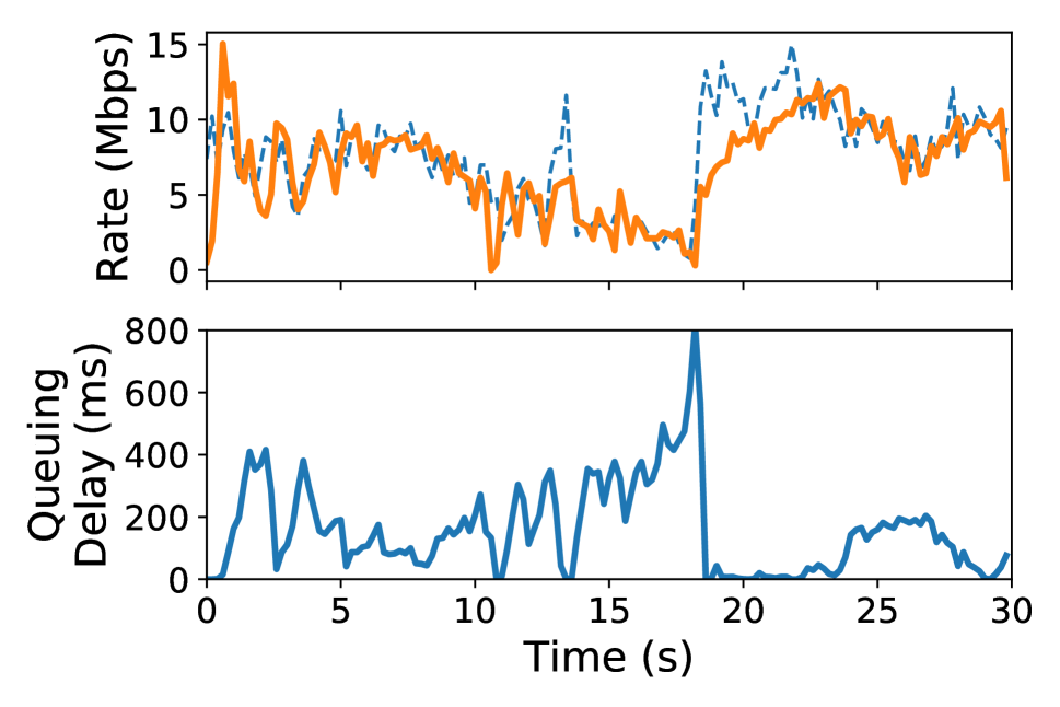
(a) BBR

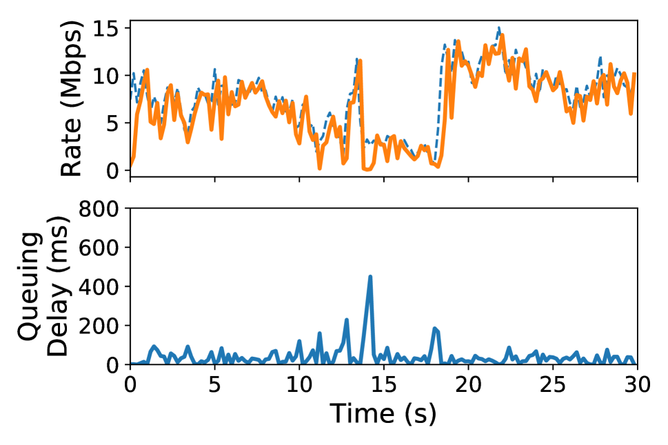
(b) ABC

Figure 14: Comparison with BBR — BBR overshoots the link capacity, causing excessive queuing. Same setup as Fig. 1.

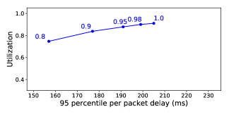
Figure 15: Impact of $\eta$ — Performance of ABC with various values of $\eta$ (target utilization). $\eta$ presents a trade-off between throughput and delay. Same setup as Fig. 1.

Appendix B Impact of $\eta$

Fig. 15 shows the performance of ABC with various values of $\eta$ on a Verizon cellular trace. Increasing $\eta$ increases the link utilization, but, also increases the delay. Thus, $\eta$ presents a trade-off between throughput and delay.

Appendix C Stability Analysis

This section establishes the stability bounds for ABC’s control algorithm (Theorem 1).

Model: Consider a single ABC link, traversed by $N$ ABC flows. Let $\mu(t)$ be the link capacity at time $t$. As $\mu(t)$ can be time-varying, we define stability as follows. Suppose that at some time $t_{0}$, $\mu(t)$ stops changing, i.e., for $t>t_{0}$ $\mu(t)=\mu$ for some constant $\mu$. We aim to derive conditions on ABC’s parameters which guarantee that the aggregate rate of the senders and the queue size at the routers will converge to certain fixed-point values (to be determined) as $t\to\infty$.

Let $\tau$ be the common round-trip propagation delay on the path for all users. For additive increase (§4.3), assume that each sender increases its congestion window by 1 every $l$ seconds. Let $f(t)$ be the fraction of packets marked accelerate, and, $cr(t)$ be the dequeue rate at the ABC router at time $t$. Let $\tau_{r}$ be time it takes accel-brake marks leaving the ABC router to reach the sender. Assuming that there are no queues other than at the ABC router, $\tau_{r}$ will be the sum of the propagation delay between ABC router and the receiver and the propagation delay between receiver and the senders. The aggregate incoming rate of ACKs across all the senders at time $t$, $R(t)$, will be equal to the dequeue rate at the router at time $t-\tau_{r}$:

$$R(t)\; =\;cr(t-\tau_{r}).$$ (9)

In response to an accelerate, a sender will send 2 packets, and, for a brake, a sender won’t send anything. In addition to responding to accel-brakes, each sender will also send an additional packet every $l$ seconds (because of AI). Therefore, the aggregate sending rate for all senders at time $t$, $S(t)$, will be

$$S(t)\; =\;R(t)\cdot 2\cdot f(t-\tau_{r})+\frac{N}{l}$$

$$=\;2cr(t-\tau_{r})f(t-\tau_{r})+\frac{N}{l}.$$ (10)

Substituting $f(t-\tau_{r})$ from Equation (2), we get

$$S(t)\; =\;tr(t-\tau_{r})+\frac{N}{l}.$$ (11)

Let $\tau_{f}$ be the propagation delay between a sender and the ABC router, and $eq(t)$ be the enqueue rate at the router at time $t$. Then $eq(t)$ is given by

$$eq(t)\; =\;S(t-\tau_{f})$$

$$=\;tr(t-(\tau_{r}+\tau_{f}))+\frac{N}{l}$$

$$=\;tr(t-\tau)+\frac{N}{l}.$$ (12)

Here, $\tau=\tau_{r}+\tau_{f}$ is the round-trip propagation delay.

Let $q(t)$ be the queue size, and, $x(t)$ be the queuing delay at time $t$:

$$x(t)\; =\;\frac{q(t)}{\mu}.$$

Ignoring the boundary conditions for simplicity ($q(t)$ must be $\geq$ 0), the queue length has the following dynamics:

$$\dot{q}(t)\; =\;eq(t)-\mu$$

$$=\;tr(t-\tau)+\frac{N}{l}-\mu$$

$$=\;\left((\eta-1)\cdot\mu+\frac{N}{l}\right)-\frac{\mu}{\delta}(x(t-\tau)-d_{t})^{+},$$

where in the last step we have used Equation (1). Therefore the dynamics of $x(t)$ can be described by:

$$\dot{x}(t)\; =\;\left((\eta-1)+\frac{N}{\mu\cdot l}\right)-\frac{1}{\delta}(x(t-\tau)-d_{t})^{+}$$

$$=\;A-\frac{1}{\delta}(x(t-\tau)-d_{t})^{+},$$ (13)

where $A=\left((\eta-1)+\frac{N}{\mu\cdot l}\right)$, and, A is a constant given a fixed number of flows $N$. The delay-differential equation in Equation (13) captures the behavior of the entire system. We use it to analyze the behavior of the queuing delay, $x(t)$, which in turn informs the dynamics of the target rate, $tr(t)$, and enqueue rate, $eq(t)$, using Equations (1) and (12) respectively.

Stability: For stability, we consider two possible scenarios 1) $A<0$, and 2) $A\geq 0$. We argue the stability in each case.

Case 1: $A<0$. In this case, the stability analysis is straightforward. The fixed point for queuing delay, $x^{*}$, is 0. From Equation (13), we get

$$\dot{x}(t)\;=\;A-\frac{1}{\delta}(x(t-\tau)-d_{t})^{+}\;\leq\;A\;<0.$$ (14)

The above equation implies that the queue delay will decrease at least as fast as $A$. Thus, the queue will go empty in a bounded amount of time. Once the queue is empty, it will remain empty forever, and the enqueue rate will converge to a fixed value. Using Equation (12), the enqueue rate can will converge to

$$eq(t)\; =\;tr(t-\tau)+\frac{N}{l}$$

$$=\;\eta\mu+\frac{N}{l}-\frac{\mu}{\delta}(x(t-\tau)-d_{t})^{+}$$

$$=\;\eta\mu+\frac{N}{l}$$

$$=\;(1+A)\mu.$$ (15)

Note that $\eta\mu<(1+A)\mu<\mu$. Since both the enqueue rate and the queuing delay converge to fixed values, the system is stable for any value of $\delta$.

Case 2: $A>0$: The fixed point for the queuing delay in this case is $x^{*}=A\cdot\delta+d_{t}$. Let $\overset{\sim}{x}(t)=x(t)-x^{*}$ be the deviation of the queuing delay from its fixed point. Substituting in Equation (13), we get

$$\dot{\overset{\sim}{x}}(t)\; =\;A-\frac{1}{\delta}(\overset{\sim}{x}(t-\tau)+A\cdot\delta)^{+}$$

$$=\;-max(-A,\frac{1}{\delta}\overset{\sim}{x}(t-\tau))$$

$$=\;-g(\overset{\sim}{x}(t-\tau)),$$ (16)

where $g(u)=\max(-A,\frac{1}{\delta}u)$ and $A>0$.

In  [50] (Corollary 3.1), Yorke established that delay-differential equations of this type are globally asymptotically stable (i.e., $\overset{\sim}{x}(t)\to 0$ as $t\to\infty$ irrespective of the initial condition), if the following conditions are met:

1. H₁: g is continuous.

2. H₂: There exists some $\alpha$, s.t. $\alpha\cdot u^{2}>ug(u)>0$ for all $u\neq 0$.

3. H₃: $\alpha\cdot\tau<\frac{3}{2}$.

The function $g(\cdot)$ trivially satisfies H₁. H₂ holds for any $\alpha\in(\frac{1}{\delta},\infty)$. Therefore, there exists an $\alpha\in(\frac{1}{\delta},\infty)$ that satisfies both H₂ and H₃ if

$$\frac{1}{\delta}\cdot\tau<\frac{3}{2}\implies\delta>\frac{2}{3}\cdot\tau.$$ (17)

This proves that ABC’s control rule is asymptotically stable if Equation (17) holds. Having established that $x(t)$ converges to $x^{*}=A\cdot\delta+d_{t}$, we can again use Equation (12) to derive the fixed point for the enqueue rate:

$$eq(t)=\eta\mu+\frac{N}{l}-\frac{\mu}{\delta}(x(t-\tau)-d_{t})^{+}\to\mu,$$ (18)

as $t\to\infty$.

Note while, we proved stability assuming that the feedback delay $\tau$ is a constant and the same value for all the senders, the proof works even if the senders have different time-varying feedback delays (see Corollary 3.2 in [50]). The modified stability criterion in this case is $\delta>\frac{2}{3}\cdot\tau^{*}$, where $\tau^{*}$ is the maximum feedback delay across all senders.

Appendix D Wi-Fi Evaluation

In this experiment we use the setup from Fig. 9(a). To emulate movement of the receiver, we model changes in MCS index as brownian motion, with values changing every 2 seconds. Fig. 16 shows throughput and $95^{th}$ percentile per packet delay for a number of schemes. Again, ABC outperforms all other schemes achieving better throughput and latency trade off.

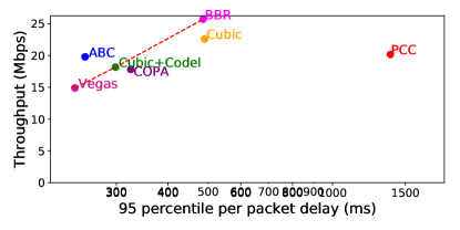
Figure 16: Throughput and $95^{th}$ percentile delay for a single user in WiFi — We model changes in MCS index as bownian motion, with values changing every 2 seconds. We limit the MCS index values to be between 3 and 7. ABC outperforms all other schemes.

Appendix E Low Delays and High Throughput

Fig. 17 shows the mean per packet delay achieved by various schemes in the experiment from Fig. 8. We observe the trend in mean delay is similar to that of 95^th percentile delay ( Fig. 8(b)). ABC achieves delays comparable to Cubic+Codel, Cubic+PIE and Copa. BBR, PCC Vivace-latency and Cubic incur 70-240% higher mean delay than ABC.

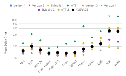
Figure 17: Utilization and mean per-packet delay across 8 different cellular network traces — On average, ABC achieves similar delays and 50% higher utilization than Copa and Cubic+Codel. BBR, PCC, and Cubic achieve slightly higher throughput than ABC, but incur 70-240% higher mean per-packet delays.

Appendix F ABC vs Explicit Control Schemes

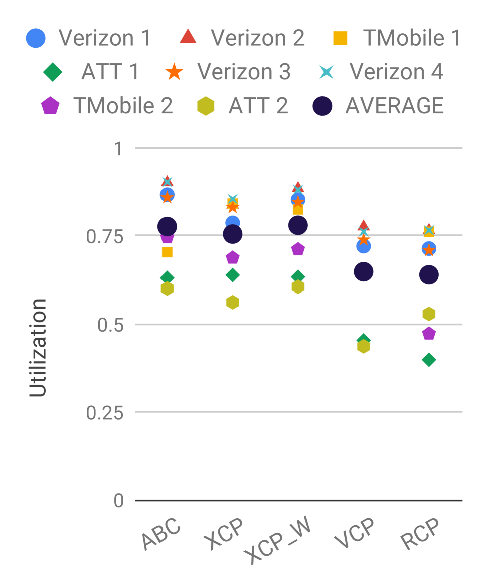
(a) Utilization

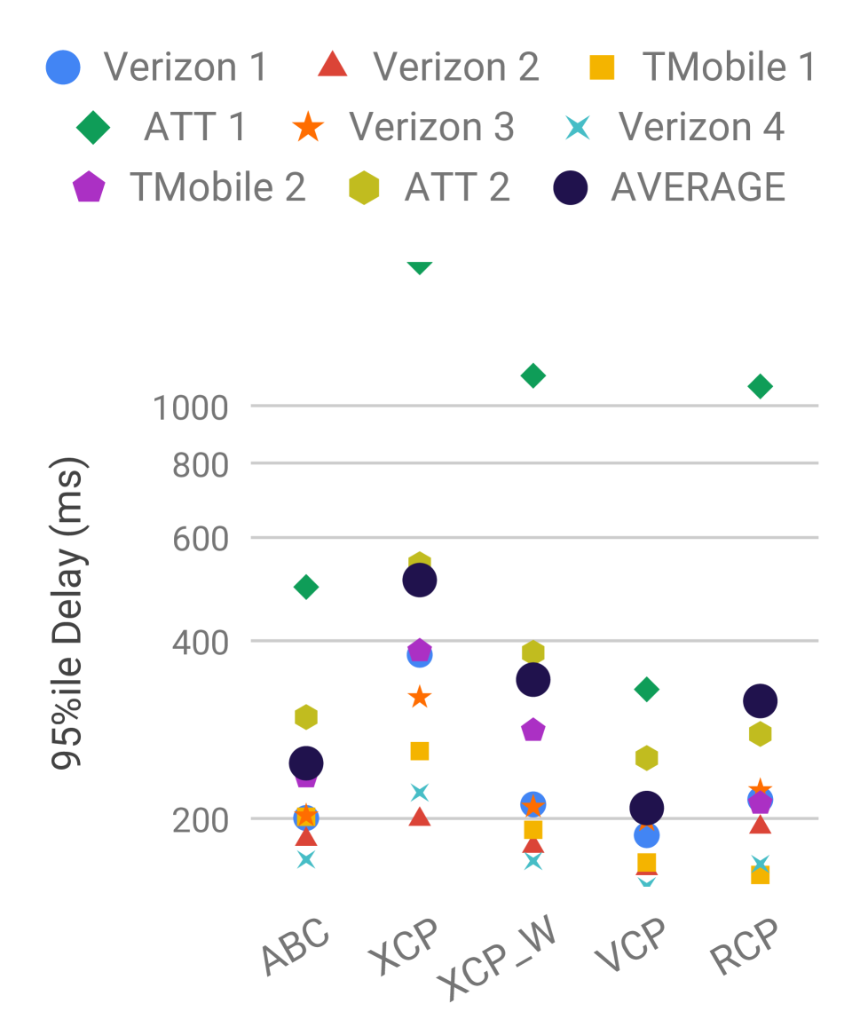
(b) Delay

Figure 18: ABC vs explicit flow control — ABC achieves similar utilization and $95^{th}$ percentile per-packet delay as XCP and XCP_w across all traces. Compared to RCP and VCP, ABC achieves 20% more utilization.

(a) ABC

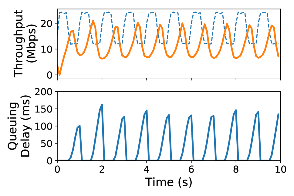
(b) RCP

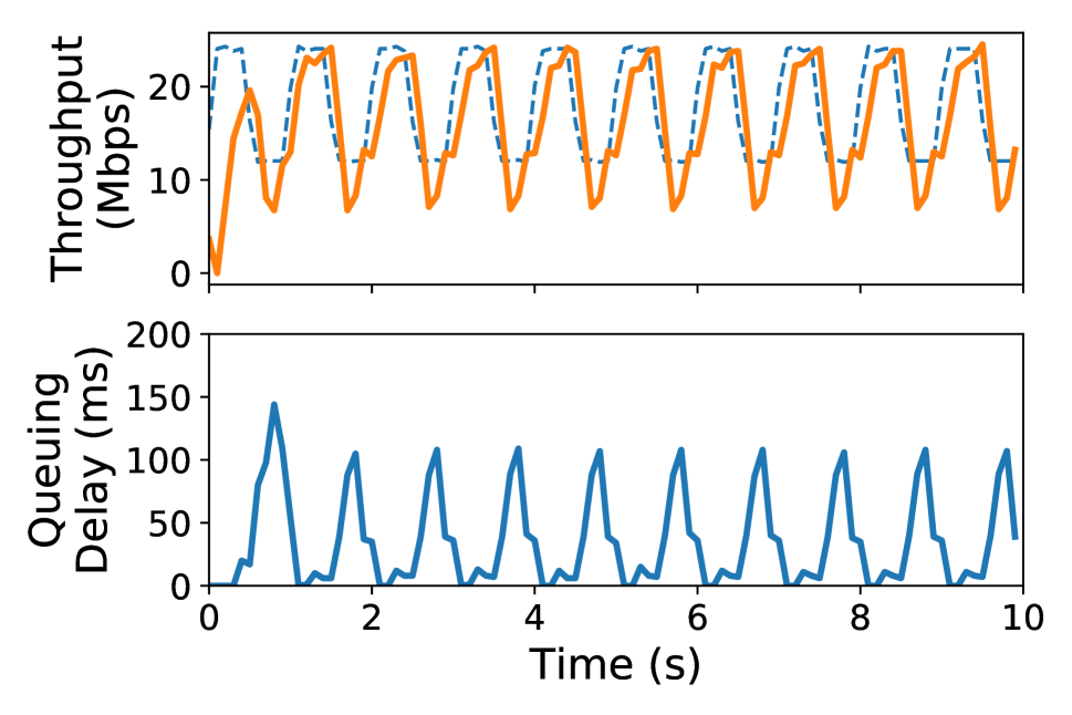
(c) XCP_w

Figure 19: Time series for explicit schemes — We vary the link capacity every 500ms between two rates 12 Mbit/sec and 24 Mbit/sec.The dashed blue in the top graph represents bottleneck link capacity. ABC and XCP_w adapt quickly and accurately to the variations in bottleneck rate, achieving close to 100% utilization. RCP is a rate base protocol and is inherently slower in reacting to congestion. When the link capacity drops, RCP takes time to drain queues and over reduces its rates, leading to under-utilization.

In this section we compare ABC’s performance with explicit congestion control schemes. We consider XCP, VCP, RCP and our modified implementation of XCP (XCP_w). For XCP and XCP_w, we used constant values of $\alpha=0.55$ and $\beta=0.4$, which the authors note are the highest permissible stable values that achieve the fastest possible link rate convergence. For RCP and VCP, we used the author-specified parameter values of $\alpha=0.5$ and $\beta=0.25$, and $\alpha=1$, $\beta=0.875$ and $\kappa=0.25$, respectively. Fig. 18 shows utilizations and mean per packet delays achieved by each of these schemes over eight different cellular link traces. As shown, ABC is able to achieve similar throughput as the best performing explicit flow control scheme, XCP_w, without using multibit per-packet feedback. We note that XCP_w’s 95^th percentile per-packet delays are 40% higher than ABC’s. ABC is also able to outperform RCP and VCP. Specifically, ABC achieves 20% higher utilization than RCP. This improvement stems from the fact that RCP is a rate based protocol (not a window based protocol)—by signaling rates, RCP is slower to react to link rate fluctuations (Figure 19 illustrates this behavior). ABC also achieves 20% higher throughput than VCP, while incurring slightly higher delays. VCP also signals multiplicative-increase/multiplicative-decrease to the sender. But unlike ABC, the multiplicative increase/decrease constants are fixed. This coarse grained feedback limits VCP’s performance on time varying links.

Fig. 19 shows performance of ABC, RCP and XCP_w on a simple time varying link. The capacity alternated between 12 Mbit/sec and 24 Mbit/sec every 500 milliseconds. ABC and XCP_w adapt quickly and accurately to the variations in bottleneck rate, achieving close to 100% utilization. RCP is a rate base protocol and is inherently slower in reacting to congestion. When the link capacity drops, RCP takes time to drain queues and over reduces its rates, leading to under-utilization.

Appendix G Other experiments

Application limited flows

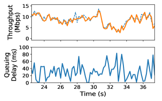
Figure 20: ABC’s robustness to flow size — With a single backlogged ABC flow and multiple concurrent application-limited ABC flows, all flows achieve high utilization and low delays.

We created a single long-lived ABC flow that shared a cellular link with 200 application-limited ABC flows that send traffic at an aggregate of 1 Mbit/s. Fig. 20 shows that, despite the fact that the application-limited flows do not have traffic to properly respond to ABC’s feedback, the ABC flows (in aggregate) are still able to achieve low queuing delays and high link utilization.

ABC’s sensitivity to network latency:

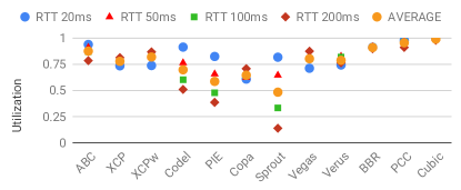
(a) Utilization

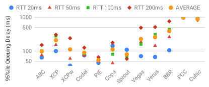
(b) per-packet queuing delay

Figure 21: Impact of propagation delay on performance — On a Verizon cellular network trace with different propagation delays, ABC achieves a better throughput/delay tradeoff than all other schemes.

Thus far, our emulation experiments have considered fixed minimum RTT values of 100 ms. To evaluate the impact that propagation delay has on ABC’s performance, we used a modified version of the experimental setup from Fig. 8. In particular, we consider RTT values of 20 ms, 50 ms, 100 ms, and 200 ms. Fig. 21 shows that, across all propagation delays, ABC is still able to outperform all prior schemes, again achieving a more desirable throughput/latency trade off. ABC’s benefits persist even though schemes like Cubic+Codel and Cubic+PIE actually improve with decreasing propagation delays. Performance with these schemes improves because bandwidth delay products decrease, making Cubic’s additive increase more aggressive (improving link utilization).

References

- [1] 3GPP technical specification for lte. https://www.etsi.org/deliver/etsi_ts/132400_132499/132450/09.01.00_60/ts_132450v090100p.pdf.
- [2] sfqCoDel. http://www.pollere.net/Txtdocs/sfqcodel.cc.
- [3] Slither.io interactive multiplayer game. http://slither.io.
- [4] F. Abrantes and M. Ricardo. XCP for shared-access multi-rate media. Computer Communication Review, 36(3):27–38, 2006.
- [5] A. Akella, S. Seshan, S. Shenker, and I. Stoica. Exploring congestion control. Technical report, CMU School of Computer Science, 2002.
- [6] M. Alizadeh, A. G. Greenberg, D. A. Maltz, J. Padhye, P. Patel, B. Prabhakar, S. Sengupta, and M. Sridharan. Data center TCP (DCTCP). In S. Kalyanaraman, V. N. Padmanabhan, K. K. Ramakrishnan, R. Shorey, and G. M. Voelker, editors, Proceedings of the ACM SIGCOMM 2010 Conference on Applications, Technologies, Architectures, and Protocols for Computer Communications, New Delhi, India, August 30 -September 3, 2010, pages 63–74. ACM, 2010.
- [7] M. Alizadeh, A. Kabbani, T. Edsall, B. Prabhakar, A. Vahdat, and M. Yasuda. Less is more: Trading a little bandwidth for ultra-low latency in the data center. In S. D. Gribble and D. Katabi, editors, Proceedings of the 9th USENIX Symposium on Networked Systems Design and Implementation, NSDI 2012, San Jose, CA, USA, April 25-27, 2012, pages 253–266. USENIX Association, 2012.
- [8] M. Allman. Tcp congestion control with appropriate byte counting (abc)", rfc 3465. 2003.
- [9] L. L. H. Andrew, S. V. Hanly, S. Chan, and T. Cui. Adaptive deterministic packet marking. IEEE Communications Letters, 10(11):790–792, 2006.
- [10] V. Arun and H. Balakrishnan. Copa: Practical delay-based congestion control for the internet. In S. Banerjee and S. Seshan, editors, 15th USENIX Symposium on Networked Systems Design and Implementation, NSDI 2018, Renton, WA, USA, April 9-11, 2018, pages 329–342. USENIX Association, 2018.
- [11] D. Bansal, H. Balakrishnan, S. Floyd, and S. Shenker. Dynamic behavior of slowly-responsive congestion control algorithms. In R. L. Cruz and G. Varghese, editors, Proceedings of the ACM SIGCOMM 2001 Conference on Applications, Technologies, Architectures, and Protocols for Computer Communication, August 27-31, 2001, San Diego, CA, USA, pages 263–274. ACM, 2001.
- [12] J. C. Bicket. Bit-rate selection in wireless networks. PhD thesis, Massachusetts Institute of Technology, 2005.
- [13] L. S. Brakmo, S. W. O’Malley, and L. L. Peterson. TCP vegas: New techniques for congestion detection and avoidance. In J. Crowcroft, editor, Proceedings of the ACM SIGCOMM ’94 Conference on Communications Architectures, Protocols and Applications, London, UK, August 31 - September 2, 1994, pages 24–35. ACM, 1994.
- [14] N. Cardwell, Y. Cheng, C. S. Gunn, S. H. Yeganeh, and V. Jacobson. BBR: congestion-based congestion control. ACM Queue, 14(5):20–53, 2016.
- [15] D. Chiu and R. Jain. Analysis of the increase and decrease algorithms for congestion avoidance in computer networks. Computer Networks, 17:1–14, 1989.
- [16] M. Dong, T. Meng, D. Zarchy, E. Arslan, Y. Gilad, B. Godfrey, and M. Schapira. PCC vivace: Online-learning congestion control. In S. Banerjee and S. Seshan, editors, 15th USENIX Symposium on Networked Systems Design and Implementation, NSDI 2018, Renton, WA, USA, April 9-11, 2018, pages 343–356. USENIX Association, 2018.
- [17] D. Ely, N. Spring, D. Wetherall, S. Savage, and T. Anderson. Robust congestion signaling. In Network Protocols, 2001. Ninth International Conference on, pages 332–341. IEEE, 2001.
- [18] F. Fainelli. The openwrt embedded development framework. In Proceedings of the Free and Open Source Software Developers European Meeting, 2008.
- [19] S. Floyd and V. Jacobson. Random early detection gateways for congestion avoidance. IEEE/ACM Trans. Netw., 1(4):397–413, 1993.
- [20] R. Fonseca, G. Porter, R. Katz, S. Shenker, and I. Stoica. Ip options are not an option. University of California at Berkeley, Technical Report UCB/EECS-2005-24, 2005.
- [21] B. Ginzburg and A. Kesselman. Performance analysis of a-mpdu and a-msdu aggregation in ieee 802.11 n. In Sarnoff symposium, 2007 IEEE, pages 1–5. IEEE, 2007.
- [22] P. Goyal, M. Alizadeh, and H. Balakrishnan. Rethinking congestion control for cellular networks. In S. Banerjee, B. Karp, and M. Walfish, editors, Proceedings of the 16th ACM Workshop on Hot Topics in Networks, Palo Alto, CA, USA, HotNets 2017, November 30 - December 01, 2017, pages 29–35. ACM, 2017.
- [23] S. Ha, I. Rhee, and L. Xu. CUBIC: a new tcp-friendly high-speed TCP variant. Operating Systems Review, 42(5):64–74, 2008.
- [24] J. C. Hoe. Improving the start-up behavior of a congestion control scheme for TCP. In D. Estrin, S. Floyd, C. Partridge, and M. Steenstrup, editors, Proceedings of the ACM SIGCOMM 1996 Conference on Applications, Technologies, Architectures, and Protocols for Computer Communication, Stanford, CA, USA, August 26-30, 1996, pages 270–280. ACM, 1996.
- [25] M. Honda, Y. Nishida, C. Raiciu, A. Greenhalgh, M. Handley, and H. Tokuda. Is it still possible to extend tcp? In P. Thiran and W. Willinger, editors, Proceedings of the 11th ACM SIGCOMM Internet Measurement Conference, IMC ’11, Berlin, Germany, November 2-, 2011, pages 181–194. ACM, 2011.
- [26] A. Jain, A. Terzis, H. Flinck, N. Sprecher, S. Arunachalam, and K. Smith. Mobile throughput guidance inband signaling protocol. IETF, work in progress, 2015.
- [27] R. Jain. Congestion control and traffic management in ATM networks: Recent advances and a survey. Computer Networks and ISDN Systems, 28(13):1723–1738, 1996.
- [28] R. Jain, A. Durresi, and G. Babic. Throughput fairness index: An explanation. In ATM Forum contribution, volume 99, 1999.
- [29] D. Katabi, M. Handley, and C. E. Rohrs. Congestion control for high bandwidth-delay product networks. In M. Mathis, P. Steenkiste, H. Balakrishnan, and V. Paxson, editors, Proceedings of the ACM SIGCOMM 2002 Conference on Applications, Technologies, Architectures, and Protocols for Computer Communication, August 19-23, 2002, Pittsburgh, PA, USA, pages 89–102. ACM, 2002.
- [30] S. T. Kent and K. Seo. Security architecture for the internet protocol. RFC, 4301:1–101, 2005.
- [31] Z. Krämer, S. Molnár, A. Mihály, and S. Nádas. Towards multi-domain congestion control in next-generation networks. In 2019 IEEE Wireless Communications and Networking Conference (WCNC), pages 1–7. IEEE, 2019.
- [32] M. Kühlewind and R. Scheffenegger. Design and evaluation of schemes for more accurate ECN feedback. In Proceedings of IEEE International Conference on Communications, ICC 2012, Ottawa, ON, Canada, June 10-15, 2012, pages 6937–6941. IEEE, 2012.
- [33] S. S. Kunniyur and R. Srikant. Analysis and design of an adaptive virtual queue (AVQ) algorithm for active queue management. In R. L. Cruz and G. Varghese, editors, Proceedings of the ACM SIGCOMM 2001 Conference on Applications, Technologies, Architectures, and Protocols for Computer Communication, August 27-31, 2001, San Diego, CA, USA, pages 123–134. ACM, 2001.
- [34] F. Lu, H. Du, A. Jain, G. M. Voelker, A. C. Snoeren, and A. Terzis. CQIC: revisiting cross-layer congestion control for cellular networks. In J. Manweiler and R. R. Choudhury, editors, Proceedings of the 16th International Workshop on Mobile Computing Systems and Applications, HotMobile 2015, Santa Fe, NM, USA, February 12-13, 2015, pages 45–50. ACM, 2015.
- [35] A. Metwally, D. Agrawal, and A. El Abbadi. Efficient computation of frequent and top-k elements in data streams. In T. Eiter and L. Libkin, editors, Database Theory - ICDT 2005, 10th International Conference, Edinburgh, UK, January 5-7, 2005, Proceedings, volume 3363 of Lecture Notes in Computer Science, pages 398–412. Springer, 2005.
- [36] R. Netravali, A. Sivaraman, S. Das, A. Goyal, K. Winstein, J. Mickens, and H. Balakrishnan. Mahimahi: Accurate record-and-replay for HTTP. In S. Lu and E. Riedel, editors, 2015 USENIX Annual Technical Conference, USENIX ATC ’15, July 8-10, Santa Clara, CA, USA, pages 417–429. USENIX Association, 2015.
- [37] K. M. Nichols and V. Jacobson. Controlling queue delay. Commun. ACM, 55(7):42–50, 2012.
- [38] R. Pan, P. Natarajan, C. Piglione, M. S. Prabhu, V. Subramanian, F. Baker, and B. VerSteeg. PIE: A lightweight control scheme to address the bufferbloat problem. In IEEE 14th International Conference on High Performance Switching and Routing, HPSR 2013, Taipei, Taiwan, July 8-11, 2013, pages 148–155. IEEE, 2013.
- [39] I. A. Qazi, L. Andrew, and T. Znati. Incremental deployment of new ecn-compatible congestion control. In Proc. PFLDNeT, 2009.
- [40] I. A. Qazi, L. L. H. Andrew, and T. Znati. Congestion control with multipacket feedback. IEEE/ACM Trans. Netw., 20(6):1721–1733, 2012.
- [41] I. A. Qazi, T. Znati, and L. L. H. Andrew. Congestion control using efficient explicit feedback. In INFOCOM 2009. 28th IEEE International Conference on Computer Communications, Joint Conference of the IEEE Computer and Communications Societies, 19-25 April 2009, Rio de Janeiro, Brazil, pages 10–18. IEEE, 2009.
- [42] K. K. Ramakrishnan, S. Floyd, and D. L. Black. The addition of explicit congestion notification (ECN) to IP. RFC, 3168:1–63, 2001.
- [43] L. Ravindranath, J. Padhye, R. Mahajan, and H. Balakrishnan. Timecard: controlling user-perceived delays in server-based mobile applications. In M. Kaminsky and M. Dahlin, editors, ACM SIGOPS 24th Symposium on Operating Systems Principles, SOSP ’13, Farmington, PA, USA, November 3-6, 2013, pages 85–100. ACM, 2013.
- [44] C. Tai, J. Zhu, and N. Dukkipati. Making large scale deployment of RCP practical for real networks. In INFOCOM 2008. 27th IEEE International Conference on Computer Communications, Joint Conference of the IEEE Computer and Communications Societies, 13-18 April 2008, Phoenix, AZ, USA, pages 2180–2188. IEEE, 2008.
- [45] A. Tirumala, F. Qin, J. Dugan, J. Ferguson, and K. Gibbs. Iperf: The TCP/UDP bandwidth measurement tool. http://dast.nlanr.net/Projects, 2005.
- [46] Z. Wang, Z. Qian, Q. Xu, Z. M. Mao, and M. Zhang. An untold story of middleboxes in cellular networks. In S. Keshav, J. Liebeherr, J. W. Byers, and J. C. Mogul, editors, Proceedings of the ACM SIGCOMM 2011 Conference on Applications, Technologies, Architectures, and Protocols for Computer Communications, Toronto, ON, Canada, August 15-19, 2011, pages 374–385. ACM, 2011.
- [47] K. Winstein, A. Sivaraman, and H. Balakrishnan. Stochastic forecasts achieve high throughput and low delay over cellular networks. In N. Feamster and J. C. Mogul, editors, Proceedings of the 10th USENIX Symposium on Networked Systems Design and Implementation, NSDI 2013, Lombard, IL, USA, April 2-5, 2013, pages 459–471. USENIX Association, 2013.
- [48] Y. Xia, L. Subramanian, I. Stoica, and S. Kalyanaraman. One more bit is enough. In R. Guérin, R. Govindan, and G. Minshall, editors, Proceedings of the ACM SIGCOMM 2005 Conference on Applications, Technologies, Architectures, and Protocols for Computer Communications, Philadelphia, Pennsylvania, USA, August 22-26, 2005, pages 37–48. ACM, 2005.
- [49] X. Xie, X. Zhang, S. Kumar, and L. E. Li. pistream: Physical layer informed adaptive video streaming over LTE. In S. Fdida, G. Pau, S. K. Kasera, and H. Zheng, editors, Proceedings of the 21st Annual International Conference on Mobile Computing and Networking, MobiCom 2015, Paris, France, September 7-11, 2015, pages 413–425. ACM, 2015.
- [50] J. A. Yorke. Asymptotic stability for one dimensional differential-delay equations. Journal of Differential equations, 7(1):189–202, 1970.
- [51] Y. Zaki, T. Pötsch, J. Chen, L. Subramanian, and C. Görg. Adaptive congestion control for unpredictable cellular networks. In S. Uhlig, O. Maennel, B. Karp, and J. Padhye, editors, Proceedings of the 2015 ACM Conference on Special Interest Group on Data Communication, SIGCOMM 2015, London, United Kingdom, August 17-21, 2015, pages 509–522. ACM, 2015.