A still unsettled issue in the nucleon spin decomposition problem : On the role of surface terms and gluon topology

Abstract

In almost all the past analyses of the decomposition of the nucleon spin into its constituents, surface terms are simply assumed to vanish and not to affect the integrated sum rule of the nucleon spin. However, several authors claim that neglect of surface terms is not necessarily justified, especially owing to possible nontrivial topological configuration of the gluon field in the QCD vacuum. There also exist some arguments indicating that the nontrivial gluon topology would bring about a delta-function type singularity at zero Bjorken variable into the longitudinally polarized gluon distribution function, thereby invalidating a naive partonic sum rule for the total nucleon spin. In the present paper, we carefully examine the role of surface terms in the nucleon spin decomposition problem. We shall argue that surface terms do not prevent us from obtaining a physically meaningful decomposition of the nucleon spin. In particular, we demonstrate that nontrivial topology of the gluon field would not bring about a delta-function type singularity into the longitudinally polarized gluon distribution functions. We also make some critical comments on the recent analyses of the role of surface terms in the density level decomposition of the total nucleon angular momentum as well as that of the total photon angular momentum.

1 Introduction

How to decompose the net spin of the nucleon into its intrinsic spin and orbital angular momentum parts of quarks and gluons is one of the fundamental problem of quantum chromodynamics (QCD). (See LL2014 ,Waka2014 for reviews.) Popular for a long time were the two decompositions known as the Jaffe-Manohar decomposition JM1990 and the Ji-decomposition Ji1997 , both of which have their own merits and demerits. The Jaffe-Manohar decomposition offers a complete decomposition of the nucleon spin into the spin and orbital parts of quarks and gluons, but it is not a gauge-invariant decomposition. On the other hand, the Ji decomposition is a manifestly gauge-invariant decomposition at the cost of giving up the decomposition of the total gluon angular momentum into its spin and orbital parts. After long and intense debates (see, for example, LL2014 ,Waka2014 for review), many researchers now believe that the Jaffe-Manohar decomposition can be made gauge-invariant at least formally by introducing the concept of the physical component of the gauge field first introduced into the problem by Chen et al. Chen2008 ,Chen2009 . However, if one is allowed to use the idea of the physical component of the gauge field, the total gluon angular momentum can also be decomposed gauge-invariantly into its spin and orbital parts. As a consequence, we are led to two complete gauge-invariant decomposition of the nucleon spin. The one is the improved Jaffe-Manohar decomposition BJ1998 , which belongs to the decomposition of canonical type, and the other is an extension of the Ji-decomposition, which we call the decomposition of mechanical (or kinetic) type Waka2010 ,Waka2011 . (We recall, however, that these two types of decomposition has totally different physical contents. What reflects the intrinsic spin structure of the nucleon is the mechanical type decomposition not the canonical type one, as throughly explained in the recent papers Waka2015 ,Waka2016 . See also Waka2013 .)

It is important to recognize the fact that different decompositions mentioned above are related to each other by the addition or subtraction of surface terms. Little attention has been paid to these surface terms, since the surface terms were believed not to contribute to the integrated sum rule of the nucleon spin. However, several authors suspect that the surface terms may not necessarily be neglected and rather they may play some unexpected roles in the nucleon spin decomposition problem Lowdon2014 - Nayak2018B . For example, based on a rigorous field theoretical treatment of the forward nucleon matrix elements of the relevant two surface terms of the angular momentum tensor, Lowdon concluded that the forward nucleon matrix elements of these surface terms precisely cancel the corresponding matrix elements for the quark and gluon spin terms Lowdon2014 . This is a perplexing conclusion, since, if it were true, the quark and gluon spin terms do not contribute to the net nucleon spin sum rule after all, thereby bereaving the practical significance of the sum rule.

Other authors claim that the nontrivial topological configuration of the gluon field in the QCD vacuum may play an unforeseen role also in the nucleon spin decomposition problem Bass2005 - Nayak2018B . Among others, Bass insisted that the nontrivial gluon topology would bring about a delta-function type singularity at zero Bjorken variable ($x=0$) into the longitudinally polarized gluon distribution function Bass2005 ,Bass2009 . We recall that the existence of such a delta-function type singularity is already known for several quark distribution functions. For example, within the framework of perturbative QCD at the one-loop level, Burkardt and Koike suggested the existence of the delta-function singularity at $x=0$ in the twist-3 distribution functions $h_{L}(x)$ and $e(x)$ BK2002 . (See also more recent analysis AB2018 .) The existence of the delta-function singularity in the twist-3 unpolarized distribution $e(x)$ was also confirmed not only within the framework of perturbative QCD but also within the framework of nonperturbative QCD WO2003 ,ES2003 . It was confirmed also within the framework of an effective model of the nucleon, i.e. the chiral quark soliton model, based on which explicit numerical calculation of $e(x)$ was also carried out OW2004 ,Schweitzer2003 . This fact has an important phenomenological impact in the respect that the existence of the delta-function singularity in $e(x)$ means breakdown of the pion-nucleon sigma term sum rule $\int_{-\,1}^{1}\,e(x)\,dx=\bar{\sigma}=\Sigma_{\pi N}/\bar{m}$ for the experimentally accessible distribution function $e(x)$, where $\bar{\sigma}$ is the scalar charge of the nucleon, while $\Sigma_{\pi N}$ is the pion-nucleon sigma term with $\bar{m}$ being the average of the up- and down-quark masses. Similarly, if the longitudinally polarized gluon distribution has a delta-function type singularity, it has a danger of bereaving the partonic sum rule for net nucleon spin Bass2005 ,Bass2009 . It is therefore of vital importance to carefully check whether such a singularity in the longitudinally polarized gluon distribution really exists or not.

In addition to the integrated sum rule of the nucleon spin, there also exists interest in the density level decomposition of the nucleon total angular momentum as well as in the density level decomposition of the total photon angular momentum. If one is interested in the density level decomposition of the total angular momentum, one has no reason to drop these surface terms. In recent papers Leader2016 ,Leader2018 , Leader investigated the density level decomposition of the total angular momentum of a free photon beam into orbital and spin parts. On the other hand, the density level decomposition of the total angular momentum of the nucleon was addressed by Lorcé, Mantovani, and Pasquini LMP2018 . Both authors emphasized that, at the density level, an unguarded neglect of the surface terms can never be justified, because the difference of two different decompositions of the total angular momentum are just characterized by these surface terms.

Now the purpose of the present paper is to answer all the questions raised above as convincingly as possible. The paper is organized as follows. First, in sect.2, we carefully inspect Lowdon’s proof that the forward nucleon matrix element of the relevant surface terms precisely cancel the corresponding matrix elements for the quark and gluon spin terms. Next, in sect.3, we try to ask the question whether the nontrivial gluon topology really brings about the delta-function type singularity in the longitudinally polarized gluon distributions. We argue that the answer to this question critically depends on the rigorous definition of the longitudinally polarized gluon distribution, which has been left in unclear status for a long time. In sect.4, we briefly review the essence of Leader’s paper as well as Lorcé et al.’s paper on the density level decomposition of the total angular momentum of the free photon and that of the nucleon from our own perspective. After that, we make several critical comments on their analyses and main claims. Then, in sect.5, we summarize principle conclusions drawn from the present investigation.

2 On Lowdon’s quantum field theoretical analysis of boundary terms

Lowdon’s argument starts with the following expression for the QCD angular momentum tensor Lowdon2014 , which was first written down in the paper by Jaffe and Monohar JM1990 :

$$M^{\mu\nu\lambda}_{QCD} = \frac{i}{2}\,\bar{\psi}\,\gamma^{\mu}\,(x^{\nu}\,\partial^{\lambda}-x^{\lambda}\,\partial^{\nu})\,\psi\ +\ \mbox{h.c.}$$ (1)

$$+ \frac{1}{2}\,\epsilon^{\mu\nu\lambda\rho}\,\bar{\psi}\,\gamma_{\rho}\,\gamma^{5}\,\psi\ \ \$$

$$- F^{\mu\rho a}\,(x^{\nu}\,\partial^{\lambda}-x^{\lambda}\,\partial^{\nu})\,A^{a}_{\rho}$$

$$+ F^{\mu\lambda a}\,A^{\nu a}\ +\ F^{\nu\mu a}\,A^{\lambda a}$$

$$+ \frac{1}{4}\,F^{a}_{\alpha\beta}\,F^{\alpha\beta a}\,(x^{\nu}\,g^{\mu\lambda}-x^{\lambda}\,g^{\mu\nu})$$

$$- \frac{i}{16}\,\partial_{\beta}\left[x^{\nu}\,\bar{\psi}\,\left\{\gamma^{\lambda},[\gamma^{\mu},\gamma^{\beta}]\right\}\,\psi\ -\ (\nu\leftrightarrow\lambda)\right]\ \ \ \ \$$

$$+ \partial_{\beta}\,\left(x^{\nu}\,F^{\mu\beta a}\,A^{\lambda a}\ -\ x^{\lambda}\,F^{\mu\beta a}\,A^{\nu a}\right),$$

with $a$ being the color index. If one drops the last two surface terms, the angular momentum tensor reduces to the form :

$$M^{\mu\nu\lambda}_{QCD} = \frac{i}{2}\,\bar{\psi}\,\gamma^{\mu}\,(x^{\nu}\,\partial^{\lambda}-x^{\lambda}\,\partial^{\nu})\,\psi\ +\ \mbox{h.c.}$$ (2)

$$+ \frac{1}{2}\,\epsilon^{\mu\nu\lambda\rho}\,\bar{\psi}\,\gamma_{\rho}\,\gamma^{5}\,\psi$$

$$- F^{\mu\rho a}\,(x^{\nu}\,\partial^{\lambda}-x^{\lambda}\,\partial^{\nu})\,A^{a}_{\rho}$$

$$+ F^{\mu\lambda a}\,A^{\nu a}\ +\ F^{\nu\mu a}\,A^{\lambda a}$$

$$+ \frac{1}{4}\,F^{a}_{\alpha\beta}\,F^{\alpha\beta a}\,(x^{\nu}\,g^{\mu\lambda}-x^{\lambda}\,g^{\mu\nu}),$$

which provides us with the basis of the famous Jaffe-Manohar decomposition of the nucleon spin JM1990 . Lowdon suspects the validity of this operation, and examined the advisability of neglecting the surface terms within a rigorous framework of quantum field theory. To this end, he first starts with the angular momentum charge given by

$$J^{i}_{QCD}\ \equiv\ \frac{1}{2}\,\epsilon^{ijk}\,\int d^{3}x\,M^{0jk}_{QCD}(x).$$ (3)

To be more rigorous, the angular momentum charges corresponding to deep-inelastic-scattering (DIS) observables, i.e. the first moments of the relevant parton distribution functions (PDFs), are related to the $+$-component in the light-cone coordinate not the time-component of the angular momentum tensor, i.e.

$$J^{i}_{QCD}\ \equiv\ \frac{1}{2}\,\epsilon^{ijk}\,\int d^{3}x\,M^{+jk}_{QCD}(x).$$ (4)

However, this difference is not of vital importance in our discussion below. We therefore follow Lowdon’s original expression, for simplicity.

Retaining the surface terms, he is then led to the decomposition :

$$J^{i}_{QCD}\ =\ L^{i}_{q}\ +\ S^{i}_{q}\ +\ L^{i}_{G}\ +\ S^{i}_{G}\ +\ S^{i}_{1}\ +\ S^{i}_{2},$$ (5)

where

$$L^{i}_{q} = \epsilon^{ijk}\,\int\,d^{3}x\,\left[\,\frac{i}{2}\,\bar{\psi}\,\gamma^{0}\,(x^{j}\,\partial^{k})\,\psi\ +\ \mbox{h.c.}\right],$$ (6)

$$S^{i}_{q} = \epsilon^{ijk}\,\int\,d^{3}x\,\left[\,\frac{1}{4}\,\epsilon^{0jkl}\,\bar{\psi}\,\gamma_{l}\,\gamma^{5}\,\psi\right],$$ (7)

$$L^{i}_{G} = -\,\epsilon^{ijk}\,\int\,d^{3}x\,\left[\,F^{0la}\,(x^{j}\,\partial^{k})\,A^{a}_{l}\,\right],$$ (8)

$$S^{i}_{G} = \epsilon^{ijk}\,\int\,d^{3}x\,\left[\,F^{0ka}\,A^{ja}\,\right],$$ (9)

$$S^{i}_{1} = -\,\frac{i}{16}\,\epsilon^{ijk}\,\int\,d^{3}x\,\,\partial^{l}\left[x^{j}\,\bar{\psi}\left\{\gamma^{k},[\gamma^{0},\gamma^{l}]\right\}\psi\,\right],\ \ \ \$$ (10)

$$S^{i}_{2} = \epsilon^{ijk}\,\int\,d^{3}x\,\,\partial_{l}\left(x^{j}\,F^{0la}\,A^{ka}\right).$$ (11)

Here, the first four terms correspond to the quark orbital angular momentum (OAM) term, the quark spin term, the gluon OAM term, and the gluon spin term, respectively, whereas the last two represent the surface integral terms that may vanish or may not vanish. Lowdon demonstrated that the forward nucleon matrix elements of the two surface terms do not vanish and rather that they precisely cancel the corresponding matrix elements for the quark and gluon spin terms in such a way that

$$\langle p,s\,|\,S^{i}_{1}\,|\,p,s\rangle\ =\ -\,\langle p,s\,|\,S^{i}_{q}\,|\,p,s\rangle,$$ (12)

$$\langle p,s\,|\,S^{i}_{2}\,|\,p,s\rangle\ =\ -\,\langle p,s\,|\,S^{i}_{G}\,|\,p,s\rangle,$$ (13)

where $|\,p,s\rangle$ stands for the nucleon state with momentum $p_{\mu}$ and spin $s_{\mu}$. If this conclusion of his were true, the quark and gluon spin terms do not contribute to the nucleon spin sum rule after all, so that the physical interpretation of the sum rule would be totally lost.

In view of serious impact of Lowdon’s conclusion on the nucleon spin decomposition problem, an immediate question is whether there is any oversight in his argument. One should remember that the problem of surface terms is nothing specific to the nucleon spin decomposition problem. Naturally, it also appears in the decomposition of the total photon angular momentum into its spin and orbital parts. Worthy of special mention here is the fact that the analogous cancellation between the surface integral term and the photon spin term happens also in the photon angular momentum decomposition problem. In fact, as argued by Stewart Stewart2005 , the total photon angular momentum of a free photon can also be decomposed into three pieces, i.e. the OAM part, the spin part, and the surface integral term. He showed that, if one considers a plane wave of arbitrary polarization, the surface integral term does not vanish and it precisely cancels the photon spin term. Note that this is just analogous to Lowdon’s observation in the nucleon spin case. According to Stewart, however, this is due to fairly singular nature of a plane wave that has infinite spatial extension. Realistic experiments are always carried out on beams that are of finite extent constricted by some apparatus. For such realistic photon beam, the surface integral term vanishes after spatial integration, and the decomposition of the total photon angular momentum into its spin and orbital parts has a proper interpretation.

Coming back to the nucleon spin decomposition problem, we recall that the original proof that the forward nucleon matrix element of the surface integral terms vanish was given by Jaffe and Manohar by using a plane wave nucleon state $|\,p,s\rangle$ with momentum $p_{\mu}$ and spin $s_{\mu}$ JM1990 . As emphasized by them, an oversimple analysis of the QCD angular momentum tensor using a plane wave state would easily lead to erroneous conclusions. The reason is that the forward limit of the nucleon matrix element and the spatial integral do not commute. To avoid this delicate nature of using a plane wave state, several authors advocated to use a wave packet state that has finite spatial extension SW2000 ,BLT2004 . Lowdon’s treatment is thought to be a field-theoretically more rigorous make-up of the wave packet formalism. In this sense, his conclusion that the forward matrix element of the surface integral terms do not vanish sounds a little strange to us, especially in view of our comment above on the photon spin decomposition problem. If any, where is an oversight in Lowdon’s argument? To answer this question, we need to follow more closely the core of his demonstration.

According to Lowdon, in classical theory, charges are defined as spatial integral of the time-component of some current density $j^{k}(x)$ :

$$Q\ =\ \int\,d^{3}x\,j^{0}(x).$$ (14)

In quantum field theory, however, more rigorous definition of charges should be given by

$$Q\ =\ \int\,d^{4}x\,f(x)\,j^{0}(x)\ \equiv\ j^{0}(f),$$ (15)

with use of some space-time test function $f$, which works to incorporate the space-time localization of physical states. A convenient choice of the test function can, for example, be given by

$$f(x)\ =\ \alpha(x_{0})\,f_{R}(\bm{x}),$$ (16)

with real functions $\alpha\in{\cal D}(\mathbb{R})\,(\mbox{supp}(\alpha)\subset[-\,\delta,\delta],\delta>0)$ and $f_{R}\in{\cal D}(\mathbb{R}^{3})$ satisfying

$$\int dx_{0}\,\alpha(x_{0})=1,\hskip 2.84526ptf_{R}(\bm{x})=\left\{\begin{array}[]{ll}1,&\ |\bm{x}|\ <\ R\\ 0,&\ |\bm{x}|\ >\ R\,(1+\epsilon),\\ \end{array}\right.$$ (17)

with some large enough radius $R$ and with $\epsilon>0$. On the basis of this setting, he derived a crucial relation given below for the surface integral term (or the super-potential operator) $\int\,d^{3}x\,\,\partial_{i}\left(x^{j}\,B^{k0i}(x)\right)$. It is given as

$$\langle p\,|\int d^{3}x\,\,\partial_{i}\left(x^{j}\,B^{k0i}(x)\right)|\,0\rangle$$ (23)

$$= \!\left\{\begin{array}[]{l}\ \lim_{R\rightarrow\infty}\,\int d^{3}x\,f_{R}(\bm{x})\,\langle 0\,|\,B^{k0j}(0)\,|\,0\rangle\\ \hskip 156.49014pt\mbox{for}\ p=0,\\ \ \lim_{R\rightarrow\infty}\,\int d^{4}x\,\alpha(x_{0})\,f_{R}(\bm{x})\,e^{\,i\,p_{\mu}\,x^{\mu}}\\ \hskip 11.38109pt\times\left[\langle p\,|\,B^{k0j}(0)\,|\,0\rangle\,+\ i\,p_{i}\,\langle p\,|\,x^{j}\,B^{k0i}(0)\,|\,0\rangle\right]\\ \hskip 156.49014pt\mbox{for}\ p\neq 0,\\ \end{array}\right.\ \ \ \ \$$

where $|\,p\rangle$ is some momentum eigenstate of the nucleon. Since this is the central formula leading to his remarkable conclusion, i.e. the cancellation between the surface integral terms and the quark and gluon spin terms, let us reexamine its derivation with extreme care.

We first note that the l.h.s. of Eq.(23) can be rewritten as

$$S \equiv \langle p\,|\,\int d^{3}x\,\,\partial_{i}\left(x^{j}\,B^{k0i}(x)\right)|\,0\rangle$$ (24)

$$= \langle p\,|\int d^{3}x\,\,\partial_{i}\left(x^{j}\,e^{\,i\,\hat{P}_{\mu}\,x^{\mu}}B^{k0i}(0)\,e^{\,-\,i\,\hat{P}_{\mu}\,x^{\mu}}\right)|\,0\rangle$$

$$= S_{1}\ +\ S_{2}\ +\ S_{3},$$

where

$$S_{1} = \langle p\,|\int\!d^{3}x\,\,x^{j}\,i\,\hat{P}_{i}\,e^{\,i\,\hat{P}_{\mu}\,x^{\mu}}B^{k0i}(0)\,e^{\,-\,i\,\hat{P}_{\mu}\,x^{\mu}}\,|\,0\rangle,$$ (25)

$$S_{2} = \langle p\,|\int\!d^{3}x\,\,x^{j}\,e^{\,i\,\hat{P}_{\mu}\,x^{\mu}}B^{k0i}(0)\,e^{\,-\,i\,\hat{P}_{\mu}\,x^{\mu}}(-\,i\hat{P}_{i})|\,0\rangle,\ \ \ \ \$$ (26)

$$S_{3} = \langle p\,|\int\!d^{3}x\,\,\delta_{ij}\,e^{\,i\,\hat{P}_{\mu}\,x^{\mu}}B^{k0i}(0)\,e^{\,-\,i\,\hat{P}_{\mu}\,x^{\mu}}\,|\,0\rangle,$$ (27)

with $\hat{P}_{\mu}$ being momentum operator. Using the relations $\hat{P}_{\mu}\,|\,p\rangle=p_{\mu}\,|\,p\rangle$ and $\hat{P}_{\mu}\,|\,0\rangle=0$, we immediately find that

$$S_{2}\ = \ \hskip 2.84526pt0,$$ (28)

$$S_{3}\ = \ \int\,d^{3}x\,\,e^{i\,p_{\mu}\,x^{\mu}}\,\langle p\,|\,B^{k0j}(0)\,|\,0\rangle.$$ (29)

Somewhat delicate is the first term $S_{1}$. Here, care must be paid to the non-commuting nature of the coordinate and momentum operator, i.e.

$$\left[x^{j},\,\hat{P}_{i}\right]\ =\ i\,\delta^{j}_{i}.$$ (30)

Taking care of this cation, the $S_{1}$ term can be rewritten as

$$S_{1} = \langle p\,|\int d^{3}x\left[i\,p_{i}\,x^{j}\,e^{\,i\,\hat{P}_{\mu}\,x^{\mu}}\,B^{k0i}(0)\,e^{\,-\,i\,\hat{P}_{\mu}\,x^{\mu}}\,|\,0\rangle\right.\ \ \$$ (31)

$$\hskip 19.91692pt\left.\ +\ i^{2}\,\delta^{j}_{i}\,e^{\,i\,\hat{P}_{\mu}\,x^{\mu}}\,B^{k0i}(0)\,e^{\,-\,i\,\hat{P}_{\mu}\,x^{\mu}}\,|\,0\rangle\right]|\,0\rangle$$

$$= \int\,d^{3}x\,\,e^{\,i\,p_{\mu}\,x^{\mu}}\,\,i\,p_{i}\,\langle p\,|\,x^{j}\,B^{k0j}(0)\,|\,0\rangle$$

$$\hskip 28.45274pt\ -\ \int\,d^{3}x\,e^{\,i\,p_{\mu}\,x^{\mu}}\,\langle p\,|\,B^{k0j}(0)\,|\,0\rangle.\ \ \ \ \$$

We notice that the second term of the above equation precisely cancels the $S_{3}$ term given by (29). As a consequence, we eventually get

$$S = \ S_{1}\ +\ S_{2}\ +\ S_{3}$$ (32)

$$= \int\,d^{3}x\,e^{\,i\,p_{\mu}\,x^{\mu}}\,i\,p_{i}\,\langle p\,|\,x^{j}\,B^{k0i}(0)\,|\,0\rangle.\ \ \ \ \$$

This especially means that, for $p=0$, it holds that

$$S\ =\ 0.$$ (33)

On the other hand, for $p\neq 0$, we obtain

$$S = \int\,d^{3}x\,e^{\,i\,p_{\mu}\,x^{\mu}}\,i\,p_{i}\,\langle p\,|\,x^{j}\,B^{k0i}(0)\,|\,0\rangle$$ (34)

$$= \lim_{R\rightarrow\infty}\,\int\,d^{4}x\,\alpha(x_{0})\,f_{R}(\bm{x})\,e^{\,i\,p_{\mu}\,x^{\mu}}$$

$$\hskip 56.9055pt\times\ i\,p_{i}\,\langle p\,|\,x^{j}\,B^{k0i}(0)\,|\,0\rangle.\ \ \ \ \$$

In the end, our answer can be summarized as

$$\langle p\,|\,\int\,d^{3}x\,\,\partial_{i}\left(x^{j}\,B^{k0i}(x)\right)\,|\,0\rangle$$ (38)

$$= \left\{\begin{array}[]{l}\!\hskip 17.07164pt0\hskip 133.72795pt\mbox{for}\ p=0,\\ \!\lim_{R\rightarrow\infty}\,\int\,d^{4}x\,\alpha(x_{0})\,f_{R}(\bm{x})\,e^{\,i\,p_{\mu}\,x^{\mu}}\\ \hskip 48.36967pt\times\ i\,p_{i}\,\langle p\,|\,x^{j}\,B^{k0j}(0)\,|\,0\rangle\hskip 5.69054pt\mbox{for}\ p\neq 0.\\ \end{array}\right.\ \ \ \ \$$

This answer clearly contradicts the formula (23) given by Lowdon. Note that, if our formula is correct, it immediately follows that the nucleon forward matrix element of any surface integral term always vanishes. In particular, we have

$$\langle p,s\,|\,S^{i}_{1}\,|\,p,s\rangle\ =\ 0,$$ (39)

$$\langle p,s\,|\,S^{i}_{2}\,|\,p,s\rangle\ =\ 0.$$ (40)

in contradiction with Lowdon’s conclusion. It seems that the origin of this discrepancy can be traced back to the fact that the non-commuting nature of the coordinate and momentum operators indicated by Eq.(30) was overlooked in Lowdon’s analysis. In fact, if we had discarded it, the $S_{1}$ term would become

$$S_{1}\ =\ \int\,d^{3}x\,e^{\,i\,p_{\mu}\,x^{\mu}}\,i\,p_{i}\,\langle p\,|\,x^{j}\,B^{k0i}(0)\,|\,0\rangle.$$ (41)

Combining this result with that for the $S_{3}$ term, one would then be led to Lowdon’s basic relation (23). We therefore conclude that, although based on somewhat delicate plane-wave formalism, the statement in the original analysis by Jaffe-Manohar is basically correct JM1990 . This means that the nucleon forward matrix elements of the surface integral terms vanish identically, thereby enabling us to obtain a physically meaningful nucleon spin sum rule.

3 The role of gluon topology on the boundary terms

Despite the early establishment of the concept of the gluon distribution functions in the field of deep-inelastic-scatter-
ing physics, how we can define the longitudinally polarized gluon distribution function $\Delta g(x)$ in a gauge-invariant manner remains to be a fairly delicate issue. In fact, the difficulty had first appeared in the absence of the twist-2 and gauge-invariant local gluon operator corresponding to the 1st moment of $\Delta g(x)$ in the operator-product-expansion (OPE) framework Sasaki1975 ,AR1975 . To get a clear answer to our problem, i.e. the role of surface terms in the definition of $\Delta g(x)$, we need to make clear all the delicacies left in the past attempts to provide a satisfactory definition of it.

Following the logical steps for providing a reasonable definition of the unpolarized gluon distribution in the pioneering work by Collins and Soper CS1982 , Bashinsky and Jaffe start with the following plausible field-theoretical definition of $\Delta g(x)$ in the light-cone (LC) gauge BJ1998 :

$$\Delta g(x) = \frac{1}{2}\,\int\,\frac{d\xi^{-}}{2\,\pi}\,e^{\,i\,x\,P^{+}\,\xi^{-}}$$ (42)

$$\times \langle P\,|\,2\,\mbox{Tr}\,\left\{F^{+\lambda}(0)\,\epsilon^{+-}{}_{\lambda}{}^{\nu}\,A_{\nu}(\xi^{-})\right\}|\,P\rangle.\ \ \ \$$

Here, the indices $\pm$ in the antisymmetric Levi-Civita symbol stand for the two light-like components, defined as $V^{\pm}=(V^{0}\pm V^{3})/\sqrt{2}$ for any four-vector $V^{\mu}$. On the other hand, the repeated indices $\lambda$ and $\nu$ represent the standard Lorentz indices, which are practically restricted to take two transverse components, i.e. $\lambda,\,\nu=1\ \mbox{or}\ 2$.

Substituting $e^{\,i\,x\,P^{+}\,\xi^{-}}$ by $(i\,x\,P^{+})^{-1}\,(\partial/\partial\xi^{-})\,e^{\,i\,x\,P^{+}\,\xi^{-}}$, integrating by parts, and using the identity $\frac{\partial}{\partial\xi^{-}}\,A_{\nu}=F^{+}{}_{\nu}=-F_{\nu}{}^{+}$ that holds in the LC gauge, they rewrite the above expression in the following form :

$$\Delta g(x) = \frac{i}{2\,P^{+}\,x}\,\int\,\frac{d\xi^{-}}{2\,\pi}\,e^{\,i\,x\,P^{+}\,\xi^{-}}$$ (43)

$$\times\,\langle P\,|\,2\,\mbox{Tr}\left\{F^{+\lambda}(0)\,\tilde{F}_{\lambda}{}^{+}(\xi^{-})\right\}|\,P\rangle+\left[\left.\left(\cdots\right)\right|^{\xi^{-}=+\,\infty}_{\xi^{-}=-\,\infty}\right].\hskip 17.07164pt$$

In the above expression, $\tilde{F}^{\mu\nu\alpha\beta}\equiv\frac{1}{2}\,\epsilon^{\mu\nu\alpha\beta}\,F_{\alpha\beta}$ is the dual field-strength tensor, while the second term represents the surface terms resulting from the partial integration. This expression is still incomplete in several respects. First, although Bashinsky-Jaffe gave a plausible argument that the surface terms are likely to vanish, stronger support is necessary especially in view of all the subtleties we have already pointed out. Second, although the main term of (43) is expressed only with the gluon field-strength tensor, it still is not invariant under general gauge transformations. The reason is the space-time nonlocality of the relevant gluon correlator as well as the following gauge transformation properties of field-strength tensors :

$$F^{+\lambda}(0)\ \rightarrow \ U(0)\,F^{+\lambda}(0)\,U^{\dagger}(0),$$ (44)

$$\tilde{F}_{\lambda}^{+}(\xi^{-})\ \rightarrow \ U(\xi^{-})\,\tilde{F}_{\lambda}^{+}(\xi^{-})\,U^{\dagger}(\xi^{-}).$$ (45)

Third, the above definition of $\Delta g(x)$ has a $1/x$ singularity at $x=0$. The principal-value prescription, which means the replacement $1/x\rightarrow P\,(1/x)$, is frequently adopted KT1999 , but its physics foundation is not necessarily clear enough. As we shall see below, all these problems are intricately interrelated. This means that, to get a completely satisfactory gauge-invariant definition of the longitudinally polarized gluon distribution, we are obliged to resolve all these delicacies simultaneously as well as without ambiguity.

To answer the question posed above, we find it very enlightening to remember the argument by Belistky, Ji, and Yuan on the transverse-momentum-dependent (TMD)
quark distribution functions BJY2003 . (See also BMP2003 .) As they stressed, the TMD quark distributions are known to be generally process-dependent quantities. A theoretically satisfactory definition of the TMD quark distribution corresponding to semi-inclusive DIS processes was shown to be given as

$$q_{DIS}(x,\bm{k}_{\perp}) = \frac{1}{2\,P^{+}}\,\int\,\frac{d\xi^{-}}{2\,\pi}\,\int\,\frac{d^{2}\bm{\xi}_{\perp}}{(2\,\pi)^{2}}\,e^{\,i\,x\,P^{+}\,\xi^{-}-i\,\bm{k}_{\perp}\cdot\bm{\xi}_{\perp}}$$ (46)

$$\times\,\langle P\,|\,\bar{\psi}(0^{-},\bm{0}_{\perp})\,{\cal W}_{C}[0^{-},\bm{0}_{\perp}\,;\,\xi^{-},\bm{\xi}_{\perp}]\,\psi(\xi^{-},\bm{\xi}_{\perp})\,|\,P\rangle,\ \ \ \$$

where

$${\cal W}_{C}[0^{-},\bm{0}_{\perp}\,;\,\xi^{-},\bm{\xi}_{\perp}] \equiv {\cal L}[0^{-},\bm{0}_{\perp}\,;\,+\,\infty^{-},\bm{0}_{\perp}]\,$$ (47)

$$\times\ {\cal L}[+\,\infty^{-},\,\bm{0}_{\perp}\,;\,+\,\infty^{-},\bm{\xi}_{\perp}]\,{\cal L}[+\,\infty^{-},\bm{\xi}_{\perp}\,;\,\xi^{-},\bm{\xi}_{\perp}],\ \ \$$

is the Wilson line, also called the gauge link, representing the future-pointing staple-like LC path as illustrated in Fig.1(a). (In the present paper, we reserve the notation ${\cal L}[\eta^{-},\bm{\eta}_{\perp}\,;\,\xi^{-},\bm{\xi}_{\perp}]$ as representing a Wilson-line that connects the two space-time points $(\xi^{-},\bm{\xi}_{\perp})$ and $(\eta^{-},\bm{\eta}_{\perp})$ with a straight-line path.)

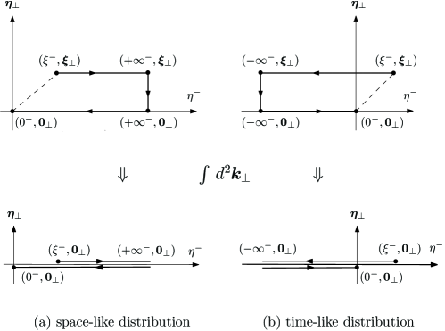
Figure 1: The left and right figures in the upper panel respectively stand for the future-pointing staple-like LC path and the past-pointing staple-like LC path simulating the final-state interaction in semi-inclusive DIS processes and the intial-state interaction in Drell-Yan processes. The lower panel represents the gauge-link structures obtained after integrating out the transverse momentum $\bm{k}_{\perp}$.

On the other hand, the TMD quark distribution corresponding to Drell-Yan processes is defined by

$$q_{DY}(x,\bm{k}_{\perp}) = \frac{1}{2\,P^{+}}\,\int\frac{d\xi^{-}}{2\,\pi}\int\frac{d^{2}\bm{\xi}_{\perp}}{(2\,\pi)^{2}}\,e^{\,i\,x\,P^{+}\,\xi^{-}-i\,\bm{k}_{\perp}\cdot\bm{\xi}_{\perp}}$$ (48)

$$\times\,\langle P\,|\,\bar{\psi}(0^{-},\bm{0}_{\perp})\,{\cal W}_{C^{\prime}}[0^{-},\bm{0}_{\perp}\,;\,\xi^{-},\bm{\xi}_{\perp}]\,\psi(\xi^{-},\bm{\xi}_{\perp})\,|\,P\rangle,\ \ \ \ \$$

where

$${\cal W}_{C^{\prime}}[0^{-},\bm{0}_{\perp}\,;\,\xi^{-},\bm{\xi}_{\perp}] \equiv {\cal L}[0^{-},\bm{0}_{\perp}\,;\,-\,\infty^{-},\bm{0}_{\perp}]\,\ \ \$$ (49)

$$\times\ {\cal L}[-\,\infty^{-},\,\bm{0}_{\perp}\,;\,-\,\infty^{-},\bm{\xi}_{\perp}]\,{\cal L}[-\,\infty^{-},\bm{\xi}_{\perp}\,;\,\xi^{-},\bm{\xi}_{\perp}],\ \ \ \ \$$

is the Wilson line representing the past-pointing staple-like LC path as illustrated in Fig.1(b).

When integrated over the transverse momentum, one gets the following expressions for the quark distribution for DIS processes

$$q_{DIS}(x) = \frac{1}{2\,P^{+}}\,\int\,\frac{d\xi^{-}}{2\,\pi}\,e^{\,i\,x\,P^{+}\,\xi^{-}}\,\langle P\,|\,\bar{\psi}(0^{-},\bm{0}_{\perp})\,\gamma^{+}\,\ \ \$$ (50)

$$\times\ {\cal L}[0^{-},\bm{0}_{\perp}\,;\,+\,\infty^{-},\bm{0}_{\perp}]\,{\cal L}[+\,\infty^{-},\bm{0}_{\perp}\,;\,\xi^{-},\bm{0}_{\perp}]$$

$$\hskip 99.58464pt\times\ \psi(\xi^{-},\bm{0}_{\perp})\,|\,P\rangle,\ \ \ \ \$$

and for the distribution for Drell-Yan processes

$$q_{DY}(x) = \frac{1}{2\,P^{+}}\,\int\,\frac{d\xi^{-}}{2\,\pi}\,e^{\,i\,x\,P^{+}\,\xi^{-}}\,\langle P\,|\,\bar{\psi}(0^{-},\bm{0}_{\perp})\,\gamma^{+}\,\ \ \ \ \$$ (51)

$$\times\ {\cal L}[0^{-},\bm{0}_{\perp}\,;\,-\,\infty^{-},\bm{0}_{\perp}]\,{\cal L}[-\,\infty^{-},\bm{0}_{\perp}\,;\,\xi^{-},\bm{0}_{\perp}]$$

$$\hskip 99.58464pt\times\ \psi(\xi^{-},\bm{0}_{\perp})\,|\,P\rangle.\ \ \$$

As Belistky, Ji, and Yuan pointed out, the unitarity of the gauge link implies that

$${\cal L}[0^{-},\bm{0}_{\perp}\,;\,+\,\infty^{-},\bm{0}_{\perp}]\,{\cal L}[+\,\infty^{-},\bm{0}_{\perp}\,;\,\xi^{-},\bm{0}_{\perp}]\ \ \ \$$ (52)

$$= {\cal L}[0^{-},\bm{0}_{\perp}\,;\,-\,\infty^{-},\bm{0}_{\perp}]\,{\cal L}[-\,\infty^{-},\bm{0}_{\perp}\,;\,\xi^{-},\bm{0}_{\perp}]$$

$$= {\cal L}[0^{-},\bm{0}_{\perp}\,;\,\xi^{-},\bm{0}_{\perp}],\ \ \ \ \$$

so that one eventually obtains

$$q_{DIS}(x) = \ q_{DY}(x)\ =\ \frac{1}{2\,P^{+}}\,\int\,\frac{d\xi^{-}}{2\,\pi}\,e^{\,i\,x\,P^{+}\,\xi^{-}}$$ (53)

$$\times\,\langle P\,|\,\bar{\psi}(0^{-},\bm{0}_{\perp})\,\gamma^{+}\,{\cal L}[0^{-},\bm{0}_{\perp}\,;\,\xi^{-},\bm{0}_{\perp}]\,\psi(\xi^{-},\bm{0}_{\perp})\,|\,P\rangle,\ \ \ \ \$$

which means that both distributions are exactly the same, thereby ensuring the universality of the $\bm{k}_{\perp}$-integrated
quark distributions.

One might expect that the same argument can be used also for showing the universality of the longitudinally polarized gluon distribution $\Delta g(x)$. Things are not so straightforward because of the $1/x$ singularity appearing in the candidates of the gauge-invariant definition of $\Delta g(x)$. We first recall that the popular choice is to use the principal-value prescription as advocated by Manohar Manohar1990 ,Manohar1991 , which gives

$$\Delta g(x) \equiv \frac{1}{4\,P^{+}}\,\int\,\frac{d\xi^{-}}{2\,\pi}\,P\,\frac{i}{x}\,e^{\,i\,x\,P^{+}\,\xi^{-}}$$ (54)

$$\times\ \langle PS_{\|}\,|\,2\,\mbox{Tr}\,\left\{\tilde{F}^{+}_{i}(0)\,{\cal L}[0^{-},\xi^{-}]\,F^{+i}(\xi^{-})\right\}|\,PS_{\|}\rangle\ \ \ \ \$$

$$+ \ (x\ \rightarrow-\,x),\ \ \ \ \$$

where the second term is included to ensure the crossing symmetry of $\Delta g(x)$. This is not the only choice, however. Possible alternatives would be given by

$$\Delta g_{post/prior}(x) \equiv \frac{1}{4\,P^{+}}\,\int\,\frac{d\xi^{-}}{2\,\pi}\,\frac{i}{x\mp i\,\epsilon}\,e^{\,i\,x\,P^{+}\,\xi^{-}}$$ (55)

$$\times\ \langle PS_{\|}\,|\,2\,\mbox{Tr}\,\left\{\tilde{F}^{+}_{i}(0^{-})\,{\cal L}[0^{-},\xi^{-}]\,F^{+i}(\xi^{-})\right\}\,|\,PS_{\|}\rangle\ \ \ \ \$$

$$+\ (x\ \rightarrow-\,x).\ \ \ \ \$$

Here the post and the prior forms of $\Delta g(x)$ respectively correspond to the choices $1/x\rightarrow 1/(x-i\,\epsilon)$ and $1/x\rightarrow 1/(x+i\,\epsilon)$. The reason of this naming is as follows. Using the mathematical identities

$$\int_{-\,\infty}^{\infty}\,dx\,\frac{i}{x-i\,\epsilon}\,e^{\,\pm\,i\,x\,P^{+}\,\xi^{-}}\ =\ -\,2\,\pi\,\theta(\pm\,\xi^{-}),$$ (56)

and

$$\int_{-\,\infty}^{\infty}\,dx\,\frac{i}{x+i\,\epsilon}\,e^{\,\pm\,i\,x\,P^{+}\,\xi^{-}}\ =\ +\,2\,\pi\,\theta(\mp\,\xi^{-}),$$ (57)

with $\theta(x)$ being the standard step function, the first moments of $\Delta g_{post}(x)$ and $\Delta g_{prior}(x)$ respectively reduce to

$$\Delta G_{post}^{(1)} \equiv \int_{-\,\infty}^{\infty}dx\,\Delta g_{post}(x)\,=\,\frac{1}{2\,P^{+}}\int d\xi^{-}\left(-\,\theta(\xi^{-})\right)$$ (58)

$$\times\,\langle PS_{\|}\,|\,2\,\mbox{Tr}\,\left\{\tilde{F}^{+}_{i}(0^{-})\,{\cal L}[0^{-},\xi^{-}]\,F^{+i}(\xi^{-})\right\}|\,PS_{\|}\rangle,\ \ \ \$$

and

$$\Delta G_{prior}^{(1)} \equiv \int_{-\,\infty}^{\infty}dx\,\Delta g_{prior}(x)\,=\,\frac{1}{2\,P^{+}}\int d\xi^{-}\left(\theta(-\,\xi^{-})\right)$$ (59)

$$\times\,\langle PS_{\|}\,|\,2\,\mbox{Tr}\,\left\{\tilde{F}^{+}_{i}(0^{-})\,{\cal L}[0^{-},\xi^{-}]\,F^{+i}(\xi^{-})\right\}|\,PS_{\|}\rangle.$$

The appearance of the factors $\theta(\xi^{-})$ in (58) and $\theta(-\,\xi^{-})$ in (59) is thought to be a reminiscence of the future-pointing and past-pointing gauge-link structures illustrated in
Fig.1(a) and Fig.1(b), which are interpreted to simulate the final-state interaction in the DIS processes and the initial-state interaction in the Drell-Yan processes. This implies the identification

$$\Delta g_{post}(x)\ \longleftrightarrow \ \Delta g_{DIS}(x),$$ (60)

$$\Delta g_{prior}(x)\ \longleftrightarrow \ \Delta g_{DY}(x).$$ (61)

The standard principal-value prescription just amounts to taking an average of the post form and the prior form :

$$\Delta g_{PV}(x)\ =\ \frac{1}{2}\,\left(\Delta g_{post}(x)\ +\ \Delta g_{prior}(x)\right).$$ (62)

We emphasize that the equality of the above three distributions is not self-evident from the beginning. Thus, the logical consequence of the consideration above is that, as candidates of physically meaningful definitions of longitudinally polarized gluon distribution, it is legitimate to start with either of the post form or the prior form depending on the process that we are considering, as Belitsky, Ji and Yuan did in their proof of universality of the $\bm{k}_{\perp}$-integrated quark distribution function BJY2003 .

Let us now investigate these two physics-based distributions in some detail. With use of the familiar mathematical identity

$$\frac{1}{x\mp i\,\epsilon}\ =\ P\,\frac{1}{x}\ \pm\ i\,\pi\,\delta(x),$$ (63)

and

$$\int_{-\,\infty}^{+\,\infty}\,dx\,\,P\,\frac{i}{x}\,\,e^{\,\pm\,i\,x\,P^{+}\,\xi^{-}}\ =\ \mp\,\pi\,\epsilon(\xi^{-}),$$ (64)

we find that the post and prior form of $\Delta g(x)$ can be expressed as

$$\Delta g_{post/prior}(x)\ =\ \Delta g_{PV}(x)\ \mp\ c\,\delta(x),$$ (65)

where

$$\Delta g_{PV}(x) = \frac{1}{2\,P^{+}}\,\int_{-\,\infty}^{\infty}\,\frac{d\xi^{-}}{2\,\pi}\,P\,\frac{i}{x}\,e^{\,i\,x\,P^{+}\,\xi^{-}}$$ (66)

$$\times\,\langle PS_{\|}\,|\,2\,\mbox{Tr}\left\{\tilde{F}^{+}_{i}(0^{-})\,{\cal L}[0^{-},\xi^{-}]\,F^{+i}(\xi^{-})\,\right\}|\,PS_{\|}\rangle,\ \ \ \ \$$

and

$$c\ = \ \frac{1}{4\,P^{+}}\,\int_{-\,\infty}^{\infty}\,d\xi^{-}\,\langle PS_{\|}\,|\,2\,\mbox{Tr}\left\{\tilde{F}^{+}_{i}(0^{-})\,{\cal L}[0^{-},\xi^{-}]\right.\ \ \$$ (67)

$$\hskip 108.12047pt\times\ \left.F^{+i}(\xi^{-})\,\right\}\,|\,PS_{\|}\rangle.$$

A key question now is therefore whether the constant $c$ vanishes or not at all.

Before answering this question, we think it instructive to look into several lower moments of $\Delta g_{post/prior}(x)$. For the first, the second, and the third moments, we find that

$$\Delta G^{(1)}_{post/prior} \equiv \int\,dx\,\,\Delta g_{post/prior}(x)$$ (68)

$$\ =\ \frac{1}{2\,P^{+}}\,\int d\xi^{-}\,\left(-\,\frac{1}{2}\,\epsilon(\xi)\right)$$

$$\times\ \langle PS_{\|}\,|\,2\,\mbox{Tr}\left\{\tilde{F}^{+}_{i}(0^{-})\,{\cal L}[0^{-},\xi^{-}]\,F^{+i}(\xi^{-})\right\}\,|\,PS_{\|}\rangle$$

$$\mp\ c,\ \ \ \ \$$

$$\Delta G^{(2)}_{post/prior} \equiv \int\,dx\,\,x\,\Delta g_{post/prior}(x)$$ (69)

$$=\ \frac{i}{4\,(P^{+})^{2}}\,\,\langle PS_{\|}\,|\,2\,\mbox{Tr}\left\{\tilde{F}^{+}_{i}(0^{-})\,F^{+i}(0^{-})\right\}\,|\,PS_{\|}\rangle$$

$$-\ \frac{i}{4\,(P^{+})^{2}}\,\,\langle PS_{\|}\,|\,2\,\mbox{Tr}\left\{\tilde{F}^{+}_{i}(0^{-})\,F^{+i}(0^{-})\right\}\,|\,PS_{\|}\rangle$$

$$\ =\ 0,$$

$$\Delta G^{(3)}_{post/prior} \equiv \int\,dx\,\,x^{2}\,\Delta g_{post/prior}(x)$$ (70)

$$=-\,\frac{1}{2\,(P^{+})^{3}}\langle PS_{\|}|\,2\,\mbox{Tr}\left\{\tilde{F}^{+}_{i}(0^{-})D^{+}F^{+i}(0^{-})\right\}|PS_{\|}\rangle,\ \ \ \$$

where $D^{+}=\partial^{+}-i\,g\,A^{+}$ is the $+$-component of the covariant derivative.

We first point out that the second moment vanishes as a cancellation of two terms emerging from the crossing symmetry of the DIS amplitude, each term of which is expressed as a nucleon matrix element of the topological charge operator of the gluon. The third moment just coincides with the expression anticipated from the operator-product expansion Sasaki1975 ,AR1975 . This is naturally the case also for higher moments. As anticipated, a subtlety remains only for the first moment, which is related to the net gluon spin contribution to the nucleon spin sum rule.

To pursue further the subtlety of the first moment of the longitudinally polarized gluon distribution, it is useful to inspect what form it reduces to in a special gauge in our problem, i.e. in the LC gauge. Using the relations ${\cal L}[0^{-},\xi^{-}]=1$ and $F^{+i}(\xi^{-})=\frac{\partial}{\partial\xi^{-}}\,A^{i}(\xi^{-})$ that holds in the LC gauge, we obtain

$$\Delta G^{(1)}_{post/prior}\ =\ \Delta G^{(1)}_{PV}\ \mp\ c,$$ (71)

where

$$\Delta G^{(1)}_{PV} = \frac{1}{2\,P^{+}}\,\langle PS_{\|}\,|\,2\,\mbox{Tr}\left\{\tilde{F}^{+}_{i}(0)\right.$$ (72)

$$\times\left.\left[A^{i}(0^{-})-\frac{1}{2}\,\left(A^{i}(+\,\infty^{-})+A^{i}(-\,\infty^{-})\right)\right]\right\}|PS_{\|}\rangle,\ \ \ \ \$$

and

$$c\ = \ \frac{1}{2\,P^{+}}\,\langle PS_{\|}\,|\,2\,\mbox{Tr}\left\{\tilde{F}^{+}_{i}(0)\right.$$ (73)

$$\hskip 22.76219pt\times\,\left.\frac{1}{2}\,\left(A^{i}(+\,\infty^{-})-A^{i}(-\,\infty^{-})\right)\right\}|\,PS_{\|}\rangle.\ \ \ \$$

Combining these, we therefore get

$$\Delta G^{(1)}_{post} = \frac{1}{2\,P^{+}}\,\langle PS_{\|}\,|\,2\,\mbox{Tr}\left\{\tilde{F}^{+}_{i}(0)\right.$$ (74)

$$\hskip 8.53581pt\times\,\left.\left(A^{i}(0^{-})-A^{i}(+\,\infty^{-})\right)\right\}|\,PS_{\|}\rangle,\ \ \$$

$$\Delta G^{(1)}_{prior} = \frac{1}{2\,P^{+}}\,\langle PS_{\|}\,|\,2\,\mbox{Tr}\left\{\tilde{F}^{+}_{i}(0)\right.$$ (75)

$$\hskip 8.53581pt\times\,\left.\left(A^{i}(0^{-})-A^{i}(-\,\infty^{-})\right)\right\}|\,PS_{\|}\rangle,\ \ \$$

We recall that the first moment in the post form essentially coincides with the expression written down by Bass inspired by the paper of Manohar Manohar1990 . (See Eq.(90) of Ref.Bass2005 .) Manohar conjectured that the gluon correlation function $\langle PS_{\|}\,|\,\mbox{Tr}\left\{\tilde{F}^{+}_{i}(0^{-})\,A^{i}(\xi^{-})\right\}\,|\,PS_{\|}\,\rangle$ would vanish as $\xi^{-}\rightarrow\pm\,\infty$. On the other hand, Bass suspects that, owing to the nontrivial topology of the gluon configuration in the QCD vacuum, this surface term might not necessarily vanish but it rather generates a delta-function type singularity at $x=0$ in the longitudinally polarized gluon distribution function $\Delta g(x)$. It must be stressed that, if $\Delta g(x)$ has such a singularity, it would invalidate a naive partonic sum rule for the net nucleon spin. It is therefore of vital importance to carefully check whether this surface term contribution vanishes or not.

Widely known remarkable fact in the LC gauge is that, $A^{i}(+\,\infty^{-})$ and $A^{i}(-\,\infty^{-})$ cannot be set to zero simultaneously, because of the Gauss law constraint $A^{i}(+\,\infty^{-})-A^{i}(-\,\infty^{-})=\int_{-\,\infty^{-}}^{+\,\infty^{-}}\,d\eta^{-}\,F^{+i}(\eta^{-})\neq 0$. Frequently used boundary condition (b.c.) for the gluon field is either of the following three :

$$A^{i}(+\,\infty^{-})\,=\,0\hskip 54.06023pt\ :\ \mbox{advanced b.c.},$$ (76)

$$A^{i}(-\,\infty^{-})\,=\,0\hskip 54.06023pt\ :\ \mbox{retarded b.c.},$$ (77)

$$A^{i}(+\,\infty^{-})+A^{i}(-\,\infty^{-})=0\ :\ \mbox{antisymmetric b.c.}\ \ \ \ \ \$$ (78)

According to Hatta Hatta2011 , how to treat the $1/x$ singularity in the gluon distribution is connected with the choices of the boundary condition for the gluon field. He defines the so-called physical component of the gluon field which transforms covariantly under gauge transformation, for three choices of the boundary condition. For retarded and advanced boundary conditions, it is defined as

$$A^{(Ret/Adv)\,i}_{phys,a}(0) = \int\,dx\,\int_{-\,\infty}^{+\,\infty}\,\frac{d\eta^{-}}{2\,\pi}\,\frac{i}{x\mp i\,\epsilon}\,e^{\,i\,x\,P^{+}\,\eta^{-}}$$ (79)

$$\hskip 42.67912pt\times\ {\cal L}_{ab}[0^{-},\eta^{-}]\,F^{+i}_{b}(\eta^{-})$$

$$= \int_{-\,\infty}^{+\,\infty}\,d\eta^{-}\,\left(\mp\,\theta(\pm\,\eta^{-})\right)\$$

$$\hskip 42.67912pt\times\ {\cal L}_{ab}[0^{-},\eta^{-}]\,F^{+i}_{b}(\eta^{-}),$$

while, for the antisymmetric (AS) boundary condition, it is defined as

$$A^{(AS)\,i}_{phys,a}(0) = \int\,dx\,\int_{-\,\infty}^{+\,\infty}\,\frac{d\eta^{-}}{2\,\pi}\,P\,\frac{i}{x}\,e^{\,i\,x\,P^{+}\,\eta^{-}}$$ (80)

$$\hskip 51.21495pt\times\,{\cal L}_{ab}[0^{-},\eta^{-}]\,F^{+i}_{b}(\eta^{-})$$

$$= \int_{-\,\infty}^{+\,\infty}\,d\eta^{-}\,\left(-\frac{1}{2}\,\epsilon(\eta^{-})\right)$$

$$\hskip 51.21495pt\times\,{\cal L}_{ab}[0^{-},\eta^{-}]\,F^{+i}_{b}(\eta^{-}).\ \ \ \ \ \$$

For each definition of the physical component, the gluon spin, or more precisely the first moment of the longitudinally polarized gluon distribution, takes the following form :

$$\Delta G^{(1)}=\frac{1}{2\,P^{+}}\,\langle PS_{\parallel}\,|\,2\,\mbox{Tr}\left\{\tilde{F}^{+}_{i}(0)\,A^{i}_{phys}(0)\right\}|PS_{\parallel}\rangle,$$ (81)

where $A^{i}_{phys}$ is the physical component in any of the retarded, advanced, or antisymmetric boundary conditions.

As is discussed above, however, the choice of the post or prior form in the definition of $\Delta g(x)$ is a physics-based operation related to the space-time structure of the Wilson line, which simulates the final-state interaction in the DIS processes or the initial-state interaction in the Drell-Yan processes. This choice can in principle be independent of the choice of the boundary condition for the gluon field at the LC spatial infinity. In fact, in either choice of the post or prior form, we have a freedom to work in the antisymmetric boundary condition for the gluon field. In fact, this is what Burkardt did in his study of the role of final-state interaction in parton orbital angular momentum Burkardt2013 . (In Waka2015 , we tried to prove the nonexistence of the delta-function singularity in $\Delta g(x)$. However, the proof given there is incomplete, because there was a confusion between the choices of the boundary condition for the gluon field and the post- and prior-form definitions of $\Delta g(x)$.)

From a practical standpoint, i.e. if one intends to solve the bound-state problem of the nucleon as a coupled quark-gluon system in some way, the antisymmetric boundary condition would be the most natural and convenient choice. For example, within the framework of the light-front quantization, Zhang and Harindranath advocated to use the antisymmetric boundary condition as a natural choice to fix the residual gauge freedom ZH1993 . They also claim that the topological winding number of the gluon field is fixed by the non-zero boundary value $A^{i}(+\,\infty^{-})=-\,A^{i}(-\,\infty^{-})$. In fact, they showed that the winding number $\Delta Q_{5}$ of the gluon field can be expressed in the following form :

$$\Delta Q_{5}\ \equiv \ n_{f}\,\frac{g^{2}}{8\,\pi^{2}}\,\int_{M}\,\mbox{Tr}\,\left(\tilde{F}^{\mu\nu}\,F_{\mu\nu}\right)$$ (82)

$$=-\,n_{f}\,\frac{g^{2}}{\pi^{2}}\,\int\,d\xi^{+}\,d^{2}\bm{\xi}_{\perp}\left.\mbox{Tr}\left(A^{-}\,[\,A^{1},A^{2}]\,\right)\,\right|_{\xi^{-}=-\,\infty}^{\xi^{-}=+\,\infty},\ \ \ \$$

with $n_{f}$ being the number of quark flavors. Note that, since the $A^{-}$ component in the light-front quantization scheme is not an independent field, $\left.A^{-}_{a}\right|_{-\,\infty}^{+\,\infty}$ is after all determined by the surface values $\left.A^{1,2}\right|_{-\,\infty}^{+\,\infty}$ of the two independent fields. This in turn means that $\Delta Q_{5}$ in Eq.(82) is determined solely by the surface values $\left.A^{1,2}\right|_{-\,\infty}^{+\,\infty}$ of the two independent fields.

As a matter of course, despite the practical advantage of using the antisymmetric boundary condition in solving the bound state problem, the choice of boundary condition in the LC gauge is in principle arbitrary, and one can choose other two boundary conditions as well. The only thing one must be careful about is that the latter choices would bring about some complexity, because the corresponding bound state wave function of the nucleon generally acquires complex phase BJY2003 . Despite this complexity, if everything is treated consistently, the final physical prediction for a gauge-invariant quantity is naturally expected to be independent of the choice of boundary condition within the LC gauge.

Now we are in a position to answer our central question. Does the coefficient $c$ of the $\delta(x)$ term vanish or not ? First, we point out that, by using the translational invariance, $c$ can be rewritten in the following form :

$$c\ = \ \frac{1}{2\,P^{+}}\,\langle PS_{\|}\,|\,2\,\mbox{Tr}\left\{\tilde{F}^{+}_{i}(0^{-})\right.$$ (83)

$$\hskip 28.45274pt\times\,\left.\frac{1}{2}\,\left(A^{i}(+\,\infty)\,-\,A^{i}(-\,\infty)\right)\right\}\,|\,PS_{\|}\rangle$$

$$= \frac{1}{2\,P^{+}}\,\langle PS_{\|}\,|\,2\,\mbox{Tr}\left\{\tilde{F}^{+}_{i}(\xi^{-})\right.$$

$$\hskip 28.45274pt\times\,\left.\frac{1}{2}\,\left(A^{i}(+\,\infty)\,-\,A^{i}(-\,\infty)\right)\right\}\,|\,PS_{\|}\rangle$$

$$= \left(1\,/\,\left(2\,P^{+}\,\int\,d\xi^{-}\right)\right).$$

$$\times \langle PS_{\|}\,|\,\int\,d\xi^{-}\,2\,\mbox{Tr}\left\{\tilde{F}^{+}_{i}(\xi^{-})\right.$$

$$\hskip 28.45274pt\left.\times\,\frac{1}{2}\,\left(A^{i}(+\,\infty)\,-\,A^{i}(-\,\infty)\right)\right\}\,|PS_{\|}\rangle.\ \ \$$

Bashinsky and Jaffe argued that this expression is expected to vanish as an infinite volume average of the derivative of a bound function BJ1998 . More tangible proof would be the following. Using the relation $\tilde{F}^{+}_{i}=g_{ij}\,\epsilon^{jk}_{\perp}\,F^{+k}$ and $F^{+k}=\frac{\partial}{\partial\xi^{-}}\,A^{k}$, the above expression can be rewritten as

$$c\ = \ \left(1\,/\,\left(2\,P^{+}\,\int\,d\xi^{-}\right)\right)$$ (84)

$$\times\ g_{ij}\,\epsilon^{jk}_{\perp}\langle PS_{\|}|\int_{-\,\infty}^{\infty}d\xi^{-}\!\frac{\partial}{\partial\xi^{-}}\,2\,\mbox{Tr}\left\{A^{k}(\xi^{-})\right.$$

$$\hskip 42.67912pt\times\,\left.\frac{1}{2}\left(A^{i}(+\,\infty)\!-\!A^{i}(-\,\infty)\right)\right\}|PS_{\|}\rangle.\ \ \ \ \$$

Since this is proportional to a nucleon forward matrix element of a surface integral term, it must vanish, as we have argued in the previous section. We therefore conclude that

$$c\ =\ 0.$$ (85)

It means that the longitudinally polarized gluon distribution does not have a delta-function-type singularity at $x=0$. This therefore ensures the existence of physically meaningful partonic sum rule for the total nucleon spin.

4 The role of surface terms on the density-level decomposition of nucleon spin

So far, our central concern has been the effect of surface terms on the integrated sum rule of the nucleon spin, and we have concluded that surface terms do not contribute to the integrated sum rule. In most cases, a similar statement holds as well also for the decomposition of the total angular momentum of the photon into its spin and orbital parts. As a matter of course, however, if we are interested in the decomposition of the total angular momentum at the density level, an unguarded neglect of the surface terms would not be justified.

In recent papers Leader2016 ,Leader2018 , Leader carried out a comparable analysis of two different decompositions of the total angular momentum of a free photon beam into orbital and spin parts at the density level. The one is the angular momentum density, which he calls the Poynting (or Belinfante) version

$$\bm{j}_{poyn}(\bm{x})\ =\ \bm{x}\times(\bm{E}\times\bm{B}),$$ (86)

with the corresponding integrated angular momentum

$$\bm{J}_{poyn}\ =\ \int\,d^{3}x\,\,\bm{x}\times(\bm{E}\times\bm{B}).$$ (87)

(Here and hereafter, the dielectric constant of vacuum $\epsilon_{0}$ is set to be unity, for simplicity.) The other is the so-called gauge-invariant-canonical (g.i.c.) version given as

$$\bm{J}_{g.i.c.}\ =\ \int\,d^{3}x\,\,\bm{j}_{g.i.c.}(\bm{x}),$$ (88)

where

$$\bm{j}_{g.i.c.}(\bm{x})\ =\ \bm{l}_{g.i.c.}(\bm{x})\ +\ \bm{s}_{g.i.c.}(\bm{x}),$$ (89)

with

$$\bm{l}_{g.i.c.}(\bm{x}) = E^{i}(\bm{x})\,(\bm{x}\times\nabla)\,A^{i}_{\perp}(\bm{x}),$$ (90)

$$\bm{s}_{g.i.c.}(\bm{x}) = \bm{E}(\bm{x})\times\bm{A}_{\perp}(\bm{x}).$$ (91)

Here, $\bm{A}_{\perp}$ represents the transverse component of the vector potential $\bm{A}$. It is a widely-known fact that $\bm{J}_{poyn}$ and $\bm{J}_{g.i.c.}$ generally differ by a surface integral term (S.T.) as

$$\bm{J}_{poyn}\ =\ \bm{J}_{g.i.c.}\ +\ \mbox{S. T.}$$ (92)

As we have already pointed out, the surface integral term vanishes in most circumstances, in which the photon fields vanish at the spatial infinity, which therefore dictates that $\bm{J}_{poyn}\ =\ \bm{J}_{g.i.c.}$. (One should keep in mind the fact, however, that there are some unusual cases where the above condition is not satisfied. For example, it was discussed in OA2014 that the surface term vanishes for “bullet-like” photon beam, but it does not for “pencil-like” photon beam that has an infinite extent along the direction of the beam.) However, it never means that these two angular momenta are the same at the density level, that is, we would generally have $\bm{j}_{poyn}\neq\bm{j}_{g.i.c.}$. As a concrete example, Leader considered a monochromatic paraxial electric field propagating in the $z$-direction ABSW1992 , which is represented as

$$\bm{E}(\bm{x})=\left(u(\bm{x}),\,v(\bm{x}),\,\frac{-\,i}{k}\left(\frac{\partial u}{\partial x}+\frac{\partial v}{\partial y}\right)\right)e^{\,i\,(k\,z\,-\,\omega\,t)},$$ (93)

with the choice

$$v(\bm{x})\ =\ i\,\sigma\,u(\bm{x})\ \ \ \mbox{with}\ \ \sigma\ =\ \pm\,1.$$ (94)

The above choice of field approximately corresponds to right and left circular polarization. For the function $u(\bm{x})$, he chooses the following form :

$$u(\rho,\phi,z)\ =\ f(\rho,z)\,e^{\,i\,l\,\phi},$$ (95)

in cylindrical coordinate $(\rho,\phi,z)$ so that it represents a vortex beam with the azimuthal mode index $l$ (the orbital angular momentum component along the $z$-direction). For the above photon beam, Allen et al. had shown that the cycle average of the $z$-component of the Poynting density, $\langle j_{poyn,z}\rangle$, per unit power modulo $\epsilon_{0}/\omega$, is given by ABSW1992

$$\langle j_{poyn,z}\rangle\ =\ l\,|u|^{2}\ -\ \frac{\sigma}{2}\,\rho\,\frac{\partial|u|^{2}}{\partial\rho}.$$ (96)

On the other hand, Leader showed that the corresponding cycle average of the g.i.c. version of angular momentum takes the following form Leader2018 :

$$\langle j_{g.i.c.,z}\rangle\ =\ l\,|u|^{2}\ +\ \sigma\,|u|^{2}.$$ (97)

Comparing these two expressions, he claims that, at the density level, the g.i.c. version, not the Poynting version, appears to show clean separation into the orbital and spin parts. He also claims that the difference of the spin density in the two versions can in principle be verified by measuring the spin angular momentum transfer to the internal angular momentum of an external atom.

These are reasonable claims as far as the photon laser physics is concerned. However, in a companion paper Leader2016 , he made a misleading overstatement as if his analysis also resolved a conflict between laser optics and particle physics. (The latter is obviously concerned with the nucleon spin decomposition problem.) The reason why his analysis is never thought to resolve the conflict between the laser optics and particle physics is very simple. It is because, while he is basically treating a photon beam in free space, a gluon in the nucleon is not a free particle. To understand the importance of this difference, i.e. the difference between free and bound (or interacting) gauge fields, the nonabelian nature of the gluon is not essential. We can stay in the abelian gauge theory, i.e. electrodynamics except that, different from Leader, we must consider photons interacting with charged particles in a nonperturbative manner.

A crucial point here is that, even in interacting theory, the total angular momentum of the photon field is given in terms of the Poynting vector as

$$\bm{J}^{\gamma}\ =\ \bm{J}_{poyn}\ =\ \int\,d^{3}x^{\prime}\,\,\bm{x}^{\prime}\times\left(\bm{E}(\bm{x}^{\prime})\times\bm{B}(\bm{x}^{\prime})\right).$$ (98)

By using the standard transverse-longitudinal decomposition of the vector potential, $\bm{A}=\bm{A}_{\perp}+\bm{A}_{\parallel}$, the electric field can also be decomposed into the transverse and longitudinal components as

$$\bm{E}\ =\ \bm{E}_{\perp}\ +\ \bm{E}_{\parallel},$$ (99)

where

$$\bm{E}_{\perp}\ =\ -\,\frac{\partial\bm{A}_{\perp}}{\partial t},\hskip 17.07164pt\bm{E}_{\parallel}\ =\ -\,\nabla A^{0}\ -\ \frac{\partial\bm{A}_{\parallel}}{\partial t}.$$ (100)

On the other hand, the magnetic field has the transverse component only, i.e. we have $\bm{B}=\bm{B}_{\perp}$, since $\bm{B}_{\parallel}=\nabla\times\bm{A}_{\parallel}=0$ by definition. The total angular momentum of the electromagnetic field can therefore be decomposed into two pieces as Waka2010

$$\bm{J}^{\gamma}\ =\ \bm{J}^{\gamma}_{\perp}\ +\ \bm{J}^{\gamma}_{\parallel},$$ (101)

where

$$\bm{J}^{\gamma}_{\perp}\ = \ \int\,d^{3}x^{\prime}\,\,\bm{x}^{\prime}\times\left(\bm{E}_{\perp}(\bm{x}^{\prime})\times\bm{B}(\bm{x}^{\prime})\right),$$ (102)

$$\bm{J}^{\gamma}_{\parallel}\ = \ \int\,d^{3}x^{\prime}\,\,\bm{x}^{\prime}\times\left(\bm{E}_{\parallel}(\bm{x}^{\prime})\times\bm{B}(\bm{x}^{\prime})\right).$$ (103)

First, after partial integration, the transverse part $\bm{J}^{\gamma}_{\perp}$ can be transformed into the form WKZZ2018 :

$$\bm{J}^{\gamma}_{\perp}\ = \ \int\,d^{3}x^{\prime}\,\,\bm{E}_{\perp}(\bm{x}^{\prime})\times\bm{A}_{\perp}(\bm{x}^{\prime})$$ (104)

$$+ \int\,d^{3}x^{\prime}\,\,E^{j}_{\perp}(\bm{x}^{\prime})\,(\bm{x}^{\prime}\times\nabla^{\prime})\,A^{j}_{\perp}(\bm{x}^{\prime})$$

$$- \int\,d^{3}x^{\prime}\,\,\nabla^{\prime j}\,\left[E^{j}_{\perp}(\bm{x}^{\prime})\,(\bm{x}^{\prime}\times\bm{A}_{\perp}(\bm{x}^{\prime}))\right].$$

The first two terms in $\bm{J}^{\gamma}_{\perp}$ respectively correspond to spin and orbital angular momentum of the photon, while the third term is the surface integral term. It is important to recognize that these three terms survive even in the free photon limit, i.e. even in the absence of the charged particle sources for the photon field. In this free photon limit, one confirms that the above decomposition just corresponds to Leader’s relation (92) for $\bm{J}_{poyn}$.

For an interacting system of photons and charged particles, however, the longitudinal part of $\bm{J}^{\gamma}$ also gives nonzero contributions. With use of partial integration supplemented with the Gauss law $\nabla^{\prime}\cdot\bm{E}_{\parallel}(\bm{x}^{\prime})=\rho(\bm{x}^{\prime})$, the longitudinal part $\bm{J}^{\gamma}_{\parallel}$ can be transformed into the following form WKZZ2018 :

$$\bm{J}^{\gamma}_{\parallel} = \int\,d^{3}x^{\prime}\,\,\rho\,(\bm{x}^{\prime}\times\bm{A}_{\perp}(\bm{x}^{\prime}))$$ (105)

$$+ \int\,d^{3}x^{\prime}\,\,\nabla^{\prime j}\,\left[(\nabla^{\prime j}\,A^{0}(\bm{x}^{\prime}))\,(\bm{x}^{\prime}\times\bm{A}_{\perp}(\bm{x}^{\prime}))\right]$$

$$- \int\,\,d^{3}x^{\prime}\,\,\nabla^{\prime j}\,\left[A^{0}(\bm{x}^{\prime})\,(\bm{x}^{\prime}\times\nabla^{\prime})\,A^{j}_{\perp}(\bm{x}^{\prime})\right]$$

$$- \int\,d^{3}x^{\prime}\,\,\nabla^{\prime}\times(A^{0}(\bm{x}^{\prime})\,\bm{A}_{\perp}(\bm{x}^{\prime})).$$

Here, aside from the first term, the remaining three terms are all surface integral terms. By using the expression for the charge density $\rho(\bm{x}^{\prime})=q\,\delta^{3}(\bm{x}^{\prime}-\bm{x})$ with $\bm{x}$ representing the position of a charged particle with the charge $q$, the first term of the above decomposition can also be expressed as

$$\int\,d^{3}x^{\prime}\,\,\rho(\bm{x}^{\prime})\,(\bm{x}^{\prime}\times\bm{A}_{\perp}(\bm{x}^{\prime}))\ =\ q\,(\bm{x}\times\bm{A}_{\perp}(\bm{x})).$$ (106)

This is nothing but the potential angular momentum $\bm{L}_{pot}$ introduced in Waka2010 ,Waka2011 , which has a meaning of angular momentum stored in the photon field in the presence of the charged particle sources. Note that the other three surface integral terms all contain the scalar potential $A^{0}$. Since $\rho=0$ and $A^{0}=0$ in the absence of charged particles, all the terms in $\bm{J}^{\gamma}_{\parallel}$ including the potential angular momentum term vanish, i.e. we have

$$\bm{J}^{\gamma}_{\parallel}\ \rightarrow\ 0,$$ (107)

in the free photon limit. This conversely means that, in the presence of the charged particle sources, the potential angular momentum term $\bm{L}_{pot}$ does not vanish. It rather constitutes an important piece of angular momentum contained in the Poynting (or Belinfante) version of the total angular momentum of the photon.

Since the nucleon is a composite system of color-charged quarks and gluons, if we follow exactly the same logical steps, we are naturally led to the conclusion that the total angular momentum of the gluon in the nucleon consists of the following three pieces

$$\bm{J}^{G}_{total}\ \equiv\ \bm{J}^{G}_{poyn}\ =\ \bm{J}^{G}_{spin}\ +\ \bm{L}^{G}_{g.i.c.}\ +\ \bm{L}_{pot},$$ (108)

aside from the surface integral terms, which we have already proved not to contribute to the integrated nucleon spin sum rule. Although we do not repeat here the discussion given in Waka2010 ,Waka2011 , the presence of the potential angular momentum term can also influence the decomposition of the total angular momentum of quarks. The potential angular momentum is the key quantity that leads to the existence of two physically inequivalent decompositions of the nucleon spin, i.e. the decomposition of the canonical type and that of the mechanical (or kinetic) type. In any case, it should be clear by now that mere discussion of the free photon beam would never unravel this important aspect of the spin decomposition problem in particle physics.

The role of surface terms in the decomposition of the nucleon spin at the density level was recently investigated by Lorcé, Mantovani, and Pasquini, through the analysis of the spatial distribution of angular momentum inside the nucleon LMP2018 . It is a widely-known fact that the canonical energy momentum tensor (EMT) obtained by using the Noether theorem is in general neither gauge invariant nor symmetric. Utilizing the arbitrariness of the Noether current such that one can always add any current which is conserved by itself, Belinfante and Rosenfeld proposed to add a so-called super potential term to the definition of both the EMT and the angular momentum tensor Belinfante1939 ,Belinfante1940 , Rosenfeld1940 :

$$T^{\mu\nu}_{Bel}(x)\ = \ T^{\mu\nu}_{can}(x)\ +\ \partial_{\lambda}\,\Sigma^{\lambda\mu\nu}(x),$$ (109)

$$J^{\mu\alpha\beta}_{Bel}(x)\ = \ J^{\mu\alpha\beta}_{can}(x)$$ (110)

$$+ \partial_{\lambda}\left[x^{\alpha}\,\Sigma^{\lambda\mu\beta}(x)\ -\ x^{\beta}\,\Sigma^{\lambda\mu\alpha}(x)\right].\ \ \ \$$

where

$$\Sigma^{\lambda\mu\nu}(x)\,=\,\frac{1}{2}\,\left[S^{\lambda\mu\nu}(x)\,+\,S^{\mu\nu\lambda}(x)\,-\,S^{\nu\lambda\mu}(x)\right].$$ (111)

Here, $T^{\mu\nu}_{can}$ and $J^{\mu\alpha\beta}_{can}$ respectively stand for the canonical EMT and the canonical angular momentum tensor, while $S^{\lambda\mu\nu}(x)$ is spin density operator that is antisymmetric with respect to the last two indices $\mu$ and $\nu$, i.e.

$$S^{\lambda\nu\mu}(x)\ =\ -\,S^{\lambda\mu\nu}(x).$$ (112)

This enables them to obtain gauge invariant and symmetric EMT and the gauge invariant angular momentum tensor with desired symmetries. It is usually believed that the requirement of symmetric EMT is motivated by general relativity. Alternatively, one can say that the graviton couples only to the symmetric part of EMT of matter field. According to Lorcé et al, however, there is no reason, from particle physics perspective, to drop the antisymmetric part from the EMT. A key observation in their analysis is then as follows. From the conservation of both the EMT and the angular momentum tensor, it follows that the EMT can generally be asymmetric, the antisymmetric part being given by the divergence of the spin density tensor $S^{\mu\alpha\beta}$,

$$T^{[\alpha\beta]}(x)\ =\ -\,\partial_{\mu}\,S^{\mu\alpha\beta}(x),$$ (113)

where $a^{[\mu}b^{\nu]}=a^{\mu}\,b^{\nu}-a^{\nu}\,b^{\mu}$.

By some strategical reason, instead of starting from the canonical EMT, their analysis starts with the Belinfante-improved form of the quark and gluon parts of EMTs given by

$$T^{\mu\nu}_{Bel,q}(x)\ = \ \frac{1}{4}\,\bar{\psi}(x)\,\gamma^{\{\mu}\,i\,{\overset{\leftrightarrow}{D}}\,^{\nu\}}\,\psi(x),$$ (114)

$$T^{\mu\nu}_{Bel,G}(x)\ = \ -\,2\,\mbox{Tr}\left[F^{\mu\lambda}(x)\,F^{\nu}_{\lambda}(x)\right]$$ (115)

$$\ +\ \frac{1}{2}\,g^{\mu\nu}\,\mbox{Tr}\left[F^{\rho\sigma}(x)\,F_{\rho\sigma}(x)\right],\hskip 17.07164pt$$

and the corresponding angular momentum tensor

$$J^{\mu\alpha\beta}_{Bel,q}(x)\ = \ x^{\alpha}\,T^{\mu\beta}_{Bel,q}(x)\ -\ x^{\beta}\,T^{\mu\alpha}_{Bel,q}(x),$$ (116)

$$J^{\mu\alpha\beta}_{Bel,G}(x)\ = \ x^{\alpha}\,T^{\mu\beta}_{Bel,G}(x)\ -\ x^{\beta}\,T^{\mu\alpha}_{Bel,G}(x),\ \ \ \$$ (117)

where $a^{\{\mu}b^{\nu\}}=a^{\mu}\,b^{\nu}+a^{\nu}\,b^{\mu}$ and $\overset{\leftrightarrow}{D}=\frac{1}{2}\,\left(\overset{\rightarrow}{D}-\overset{\leftarrow}{D}\right)$.

As a first step, they compared the quark part of the Belinfante-improved EMT with the EMT in what they call the kinetic form given as

$$T^{\mu\nu}_{kin,q}(x)\ = \ \frac{1}{2}\,\bar{\psi}(x)\,\gamma^{\mu}\,i\,{\overset{\leftrightarrow}{D}}\,^{\nu}\,\psi(x).$$ (118)

They notice that this kinetic EMT is obtained from the Belinfante-improved EMT by adding an antisymmetric piece as

$$T^{\mu\nu}_{kin,q}(x)\ =\ T^{\mu\nu}_{Bel,q}(x)\ +\ \frac{1}{2}\,T^{[\mu\nu]}_{q}(x),$$ (119)

where

$$T^{[\alpha\beta]}_{q}(x)\ =\ -\,\partial_{\lambda}\,S^{\lambda\alpha\beta}_{q}(x),$$ (120)

with the definition of the quark spin density operator

$$S^{\lambda\alpha\beta}_{q}(x)\ =\ \frac{1}{2}\,\epsilon^{\alpha\beta\lambda\sigma}\,\bar{\psi}(x)\,\gamma_{\sigma}\,\gamma_{5}\,\psi(x).$$ (121)

Similarly, by adding the following super potential term

$$- \partial_{\lambda}\left[x^{\alpha}\,\Sigma^{\lambda\mu\beta}_{q}(x)\,-\,x^{\beta}\,\Sigma^{\lambda\mu\alpha}_{q}(x)\right]$$ (122)

$$= -\,\frac{1}{2}\,\partial_{\lambda}\left[x^{\alpha}\,S^{\lambda\mu\beta}_{q}(x)\,-\,x^{\beta}\,S^{\lambda\mu\alpha}_{q}(x)\right],\ \ \$$

to the quark part of the Belinfante-improved angular momentum tensor $J^{\mu\alpha\beta}_{Bel,q}(x)$, they obtain the relation

$$L^{\mu\alpha\beta}_{kin,q}(x)\ +\ S^{\mu\alpha\beta}_{q}(x)\ =\ J^{\mu\alpha\beta}_{Bel,q}(x)$$ (123)

$$\hskip 28.45274pt-\ \frac{1}{2}\,\partial_{\lambda}\left[x^{\alpha}\,S^{\lambda\mu\beta}_{q}(x)\ -\ x^{\beta}\,S^{\lambda\mu\alpha}_{q}(x)\right].\ \ \ \$$

Here, the first term on the l.h.s. represents the quark orbital angular momentum density tensor defined by

$$L^{\mu\alpha\beta}_{kin,q}(x)\ =\ x^{\alpha}\,T^{\mu\beta}_{kin,q}(x)\ -\ x^{\beta}\,T^{\mu\alpha}_{kin,q}(x),$$ (124)

whereas the second term on the l.h.s. is just the quark spin density tensor. Concerning the gluon part, they employ the traditional viewpoint that the total angular momentum of the gluon cannot be decomposed further into its spin and orbital parts without conflict with the gauge-invariance and the locality, so that they simply equate the kinetic and Belinfante-improved tensors for the gluon part as

$$J^{\mu\alpha\beta}_{kin,G}(x)\ =\ J^{\mu\alpha\beta}_{Bel,G}(x).$$ (125)

This immediately leads to their basic relation

$$L^{\mu\alpha\beta}_{kin,q}(x)\ +\ S^{\mu\alpha\beta}_{q}(x)\ +\ J^{\mu\alpha\beta}_{kin,G}(x)$$

$$= \,J^{\mu\alpha\beta}_{Bel,q}(x)\ +\ J^{\mu\alpha\beta}_{Bel,G}(x)$$ (126)

$$\hskip 42.67912pt-\ \frac{1}{2}\,\partial_{\lambda}\left[x^{\alpha}\,S^{\lambda\mu\beta}_{q}(x)\ -\ x^{\beta}\,S^{\lambda\mu\alpha}_{q}(x)\right].\hskip 28.45274pt$$

The l.h.s. of the above equation is nothing but the local version of the Ji decomposition, while the r.h.s. is the decomposition in the Belinfante version plus a surface term. In this way, they are led to their central observation that, at the local density level, the difference between the Ji decomposition and the Belinfante-improved version is characterized by a surface term, which is expressed with the quark spin density or the quark axial density that can in principle be related to an observable by means of neutrino-nucleon scatterings.

In order to relate the above-mentioned angular momentum densities to observables, what plays a key role are the following two quantities. The first is the nucleon matrix elements of the general asymmetric EMT parametrized by five form factors $A(t),B(t),C(t),D(t)$ and $\bar{C}(t)$ as

$$\langle p^{\prime},\bm{s}^{\prime}\,|\,T^{\mu\nu}(0)\,|\,p,\bm{s}\rangle\ =\ \bar{u}(p^{\prime},\bm{s}^{\prime})\,\left[\frac{P^{\mu}\,P^{\nu}}{M}A(t)\right.\ \ \$$ (127)

$$\hskip 8.53581pt+\ \frac{P^{\mu}\,i\,\sigma^{\nu\lambda}\,\Delta_{\lambda}}{M}\,\left(A(t)+B(t)+D(t)\right)$$

$$\hskip 8.53581pt+\ \frac{\Delta^{\mu}\,\Delta^{\nu}\ -\ g^{\mu\nu}\,\Delta^{2}}{M}\,C(t)$$

$$\hskip 8.53581pt+\ M\,g^{\mu\nu}\,\bar{C}(t)$$

$$\hskip 8.53581pt+\left.\frac{P^{\nu}\,i\,\sigma^{\mu\lambda}\,\Delta_{\lambda}}{4\,M}\,\left(A(t)+B(t)-D(t)\right)\right]u(p,\bm{s}),\ \ \ \ \ \ \$$

where $M$ is the nucleon mass, $\bm{s}$ and $\bm{s}^{\prime}$ denote the rest-frame spin of the initial and final nucleon states, respectively, and $P=(p^{\prime}+p)/2,\,\Delta=p^{\prime}-p,\,t=\Delta^{2}$. The second is the nucleon matrix elements of the quark spin operator $S^{\mu\alpha\beta}_{q}(0)$ parametrized as

$$\langle p^{\prime},\bm{s}^{\prime}\,|\,S^{\mu\alpha\beta}_{q}(0)\,|\,p,\bm{s}\rangle\!\! = \!\!\frac{1}{2}\,\epsilon^{\mu\alpha\beta\lambda}$$ (128)

$$\times\ \bar{u}(p^{\prime},\bm{s}^{\prime})\,\left[\gamma_{\lambda}\,\gamma_{5}\,G^{q}_{A}(t)\ +\ \frac{\Delta_{\lambda}\,\gamma_{5}}{2\,M}\,G^{q}_{P}(t)\right]\,u(p,\bm{s}),\hskip 22.76219pt$$

where $G^{q}_{A}(t)$ and $G^{q}_{P}(t)$ are the axial-vector and induced pseudoscalar form factors.

As was pointed out in their paper, the EMT form factors $A(t),B(t)$ and $C(t)$ can be related to leading-twist generalized parton distributions (GPDs), and they are in principle be observables. The form factor $\bar{C}(t)$, which has a relation to the trace of EMT, can be extracted from $\pi N$ scattering amplitudes and so on. Finally, the remaining form factor $D(t)$, which is connected with the non-symmetric part of EMT, can be related to the axial-vector form factor as $D_{q}(t)=-\,G^{q}_{A}(t)$, which is measurable from neutrino-nucleon scatterings. Using the above parametrization of the nucleon matrix elements of the EMT as well as the quark spin operator, Lorcé et al. analyzed several spatial distributions of angular momentum in the Belinfante form and in the kinetic forms. They are spatial distributions of angular momentum in instant form, the corresponding 2-dimensional distributions in the so-called elastic frame, and the analogous distributions in light-front form. Here, we explain the point of their argument by taking the distributions in light-front form as an example.

They start with the definition of the kinetic OAM distribution of quarks in four dimensional position space

$$\langle L^{z}\rangle(x)\ =\ \epsilon^{3jk}\,x^{j}_{\perp}\,\int\,\frac{d^{2}\bm{\Delta}_{\perp}\,d\Delta^{+}}{(2\,\pi)^{2}}\,e^{\,i\,\Delta\cdot x}\,\langle T^{+k}\rangle_{LF},$$ (129)

where

$$\langle T^{\mu\nu}\rangle_{LF}\ \equiv\ \frac{\langle p^{\prime},\bm{s}\,|\,T^{\mu\nu}(0)\,|\,p,\bm{s}\rangle}{2\,\sqrt{p^{\prime+}\,p^{+}}}.$$ (130)

The corresponding impact parameter distributions in the light-front formalism are defined in the Drell-Yan (DY) frame where $\Delta^{+}=0$ and $\bm{P}_{\perp}=0$, which amounts to integrating out the four-dimensional distributions over the light-front coordinate $x^{-}$. In this frame, the dependence on the light-front time $x^{+}$ also drops out. Then, with the identification $\bm{x}_{\perp}\rightarrow\bm{b}_{\perp}$, the impact-parameter distributions of kinetic OAM and spin can be represented as

$$\langle L^{z}\rangle(\bm{b}_{\perp})\!\! = \!\!s^{z}\,\int\,\frac{d^{2}\bm{\Delta}_{\perp}}{(2\,\pi)^{2}}\,e^{\,-\,i\,\bm{\Delta}_{\perp}\cdot\bm{b}_{\perp}}$$ (131)

$$\hskip 28.45274pt\times\left[L(t)\ +\ t\,\frac{dL(t)}{dt}\right]_{t=-\,\bm{\Delta}^{2}_{\perp}},\ \ \ \ \$$

$$\langle S^{z}\rangle(\bm{b}_{\perp})\!\! = \!\!\frac{1}{2}\,s^{z}\,\int\,\frac{d^{2}\bm{\Delta}_{\perp}}{(2\,\pi)^{2}}\,e^{\,-\,i\,\bm{\Delta}_{\perp}\cdot\bm{b}_{\perp}}\,G_{A}(-\,\bm{\Delta}^{2}_{\perp}).\ \ \ \ \$$ (132)

Here, $L(t)$ is a combination of the EMT form factors given by

$$L(t)\ =\ \frac{1}{2}\,\left[A(t)+B(t)+D(t)\right],$$ (133)

while $G_{A}(t)$ is the axial-vector form factor.

The corresponding impact-parameter distributions of Belinfante improved total angular momentum and total divergence (surface term) are given by

$$\langle J^{z}_{Bel}\rangle(\bm{b}_{\perp}) = s^{z}\,\int\,\frac{d^{2}\Delta_{\perp}}{(2\,\pi)^{2}}\,e^{\ -\,i\,\bm{\Delta}_{\perp}\cdot\bm{b}_{\perp}}$$ (134)

$$\hskip 28.45274pt\times\left[J(t)\ +\ t\,\frac{dJ(t)}{dt}\right]_{t=-\,\bm{\Delta}^{2}_{\perp}},\ \ \ \ \ \ \$$

$$\langle M^{z}\rangle(\bm{b}_{\perp}) = -\,\frac{1}{2}\,s^{z}\,\int\,\frac{d^{2}\Delta_{\perp}}{(2\,\pi)^{2}}\,e^{\ -\,i\,\bm{\Delta}_{\perp}\cdot\bm{b}_{\perp}}$$ (135)

$$\hskip 51.21495pt\times\left[\,t\,\frac{dG_{A}(t)}{dt}\right]_{t=-\,\bm{\Delta}^{2}_{\perp}}.$$

Here $J(t)$ is another combination of EMT for factors given by

$$J(t)\ =\ \frac{1}{2}\,\left[A(t)+B(t)\right].$$ (136)

Using the relation $J(t)\,-\,L(t)=-\frac{1}{2}\,D(t)=\frac{1}{2}\,G_{A}(t)$, one can directly check that the following relation holds

$$\langle L^{z}\rangle(\bm{b}_{\perp})\ +\ \langle S^{z}\rangle(\bm{b}_{\perp})\ =\ \langle J^{z}_{Bel}\rangle(\bm{b}_{\perp})\ +\ \langle M^{z}\rangle(\bm{b}_{\perp}).$$ (137)

This gives the relation between the local version of quark part of the nucleon angular momentum in the Ji decomposition Ji1997 and that of the Belinnfante version supplemented with the surface density term. Now, their main assertion is summarized in the following phrase. “While superpotential terms do not play any role at the level of integrated quantities, it is of crucial importance to keep track of them at the level of distributions”. This would be a reasonable statement in itself. Nonetheless, several comments are in order on their main claims.

First, it would certainly be true that the decomposition based on the Belinfante-improved EMT and that in the kinetic version give different forms of angular momentum decomposition at the density level. It is also true that the impact-parameter distributions $\langle L^{z}\rangle(\bm{b}_{\perp})$, $\langle S^{z}\rangle(\bm{b}_{\perp})$, $\langle J^{z}_{Bel}\rangle(\bm{b}_{\perp})$, and $\langle M^{z}\rangle(\bm{b}_{\perp})$ are all expressed in terms of the EMT form factors $A(t),B(t),D(t)$ and/or the axial-vector form factor $G_{A}(t)=-\,D(t)$. However, real observables are not the impact-parameter distributions appearing in Eq.(137), but the EMT form factors $A(t),B(t)$ and $D(t)=-\,G_{A}(t)$. Any of the impact-parameter distributions appearing in both sides of (137) are not direct observables. At the best, they may be predicted within some theoretical framework like Lattice QCD or some effective models of the nucleon, and a comparison can be made only among those theoretical predictions. In particular, although the surface term $\langle M^{z}\rangle(\bm{b}_{\perp})$ is expressed with the axial-vector form factor of the nucleon, we do not have any means to directly measure this distribution. The reason is that there is no external probe which couples to this surface density. This point is vitally different from the case of photon laser physics. Remember that, in this case, the surface term, which characterizes the difference between the two versions of photon spin density, can in principle be probed by measuring the spin angular momentum transfer to the internal angular momentum of an external photon, as emphasized by Leader.

Another remark is the following. For obtaining the kinetic decomposition or the Ji decomposition from the Belinfante-improved form, which enables the decomposition of the total angular momentum of quarks into the orbital and spin parts, Lorcé et al. added a super-potential term, which is expressed with the quark spin density tensor. According to them, this is motivated by the particle physics viewpoint that there is no reason to drop the antisymmetric part from the EMT tensor, since it has inseparable connection with the spin degrees of the particles. If so, why not include the spin density part of the gluon into the super potential term ? In fact, the relevant super potential should be

$$\Sigma^{\lambda\mu\nu}_{G}(x)\,=\,\frac{1}{2}\,\left[S^{\lambda\mu\nu}_{G}(x)\,+\,S^{\mu\nu\lambda}_{G}(x)\,-\,S^{\nu\lambda\mu}_{G}(x)\right],$$ (138)

where

$$S^{\lambda\mu\nu}_{G}(x)\ =\ -\,2\,\mbox{Tr}\left[F^{\lambda\mu}(x)\,A^{\nu}(x)\ -\ \left(\mu\leftrightarrow\nu\right)\right],$$ (139)

is the gluon spin density operator. Naturally, it is a widely-recognized fact that this expression of the gluon spin density is not gauge-invariant. However, a natural standpoint could be that the spin degrees of freedom is more important than the gauge degrees of freedom, since the former is physical, while the latter is just redundancy with little physical contents. Alternatively, one can introduce a gluon spin density tensor, which is formally gauge-invariant. This can be done by introducing the decomposition of the gluon field into its physical and pure-gauge components as $A^{\mu}=A^{\mu}_{phys}+A^{\mu}_{pure}$ as was done in Waka2010 ,Waka2011 . (We point out that the deep meaning hidden in the concept of the physical component of the gauge field can most transparently be understood through the analysis of a solvable quantum mechanical system, i.e. the Landau problem WKZ2018 .) Although these two standpoints can easily be compromised, here it is simpler to take the first standpoint, in order not to introduce unnecessary complexity into the argument. Adding the corresponding super-potential term to the gluon part of the Belinfante-improved angular momentum tensor, we readily obtain

$$J^{\mu\alpha\beta}_{kin,G}\ =\ J^{\mu\alpha\beta}_{Bel,G}\ -\ \partial_{\lambda}\left[x^{\alpha}\,\Sigma^{\lambda\mu\beta}_{G}\ -\ x^{\beta}\,\Sigma^{\lambda\mu\alpha}_{G}\right],$$ (140)

with

$$J^{\mu\alpha\beta}_{kin,G} = -\ 2\ \mbox{Tr}\left[F^{\mu\alpha}\,A^{\beta}\ -\ F^{\mu\beta}\,A^{\alpha}\right]$$ (141)

$$\ +\ 2\,\,\mbox{Tr}\left[F^{\lambda\mu}\,\left(x^{\alpha}\,\partial^{\beta}\ -\ x^{\beta}\,\partial^{\alpha}\right)\,A_{\lambda}\right]$$

$$\ +\ 2\,\,\mbox{Tr}\left[(D_{\lambda}\,F^{\lambda\mu})\,\left(x^{\alpha}\,A^{\beta}\ -\ x^{\beta}\,A^{\alpha}\right)\right]\ \ \ \$$

$$\ +\ \frac{1}{2}\,\,\mbox{Tr}\,F^{2}\,\left(x^{\alpha}\,g^{\mu\beta}\ -\ x^{\beta}\,g^{\mu\alpha}\right).$$

Here, the 1st and the 2nd term of the above equation just correspond to the spin and canonical orbital angular momentum tensors of the gluon field. The 3rd term is nothing but the tensor corresponding to the potential angular momentum, which survives only for coupled quark-gluon system. The 4th term, sometimes called the boost term, does not contribute to the angular momentum density, which is of our concern here.

Combining the above result for the gluon part with that for the quark part, we are thus led to the following decomposition of the nucleon angular momentum tensor,

$$J^{\mu\alpha\beta}_{nucleon} = L^{\mu\alpha\beta}_{kin,q}\ +\ S^{\mu\alpha\beta}_{q}\ +\ L^{\mu\alpha\beta}_{kin,G}\ +\ S^{\mu\alpha\beta}_{G}\ \ \ \$$ (142)

$$+ \ \mbox{boost},$$

where

$$L^{\mu\alpha\beta}_{kin,q}\ = \ \frac{1}{2}\,\bar{\psi}\,\gamma^{\mu}\left(x^{\alpha}\,i\,\overset{\leftrightarrow}{D}\,^{\beta}\ -\ x^{\beta}\,i\,\overset{\leftrightarrow}{D}\,^{\alpha}\right)\psi,\ \ \$$ (143)

while

$$L^{\mu\alpha\beta}_{kin,G}\ = \ 2\,\mbox{Tr}\left[F^{\lambda\mu}\,\left(x^{\alpha}\,\partial^{\beta}\ -\ x^{\beta}\,\partial^{\alpha}\right)\,A_{\lambda}\right]$$

$$+ \ 2\,\mbox{Tr}\left[\left(D_{\lambda}\,F^{\lambda\mu}\right)\,\left(x^{\alpha}\,A^{\beta}\ -\ x^{\beta}\,A^{\alpha}\right)\right]\ \ \ \$$ (144)

$$= \ \ L^{\mu\alpha\beta}_{can,G}\ \ +\ \ L^{\mu\alpha\beta}_{pot},$$

$$S^{\mu\alpha\beta}_{G}\ = -\ 2\,\mbox{Tr}\left[F^{\mu\alpha}\,A^{\beta}\ -\ F^{\mu\beta}\,A^{\alpha}\right].$$ (145)

Aside from the gauge problem of the gluon part, which can formally be eliminated by the introduction of the concept of the physical component of the gauge field, the above is precisely the decomposition which we proposed in Waka2010 ,Waka2011 as a natural extension of the Ji decomposition.

Naturally, there is a reason why Lorcé et al. did not introduce the super-potential term corresponding to the gluon spin density, aside from the problem of gauge invariance. At variance with the quark spin density term, which can be related to an observable, i.e. the axial-vector form factor of the nucleon, we do not have any means to relate the gluon spin density to a direct observable. One might think that this fact is connected with the color-gauge-variant nature of the gluon spin density. However, this understanding would not be necessarily correct. In fact, suppose that we live in a world where there exists only the electromagnetic interaction besides the strong interaction, i.e. in a world with no weak interaction. It is clear that, in the absence of external weak probe, we have no means to experimentally access the quark spin density even if the quark spin density satisfies color-gauge invariance. This implies that there is no absolute connection between the color-gauge invariance of a certain quantity and its observability. After all, what is vital for observability is the existence of external probe which couples to the quantity in question.

We emphasize that the decomposition of the total gluon angular momentum into its spin and orbital parts is a natural operation also from the standpoint of perturbative QCD. The longitudinally polarized gluon distribution as well as its first moment are well-established concepts within the framework of perturbative QCD, even though they are usually thought to be theoretical-scheme-dependent observables. At any rate, one should keep in mind the fact that various types of decomposition of the angular momentum inside the nucleon are related though an addition or subtraction of surface terms, the density of which can hardly be verified by direct measurements. This implies that discussing the density-level decomposition of the nucleon spin is a far more difficult task than discussing the integrated nucleon spin sum rule, especially if we consider its direct experimental verification seriously.

5 Conclusion

When discussing the decomposition of the nucleon spin into its constituents, it is customary to simply discard the contributions of surface terms. However, several authors issued a warning against silent neglect of the surface terms in the nucleon spin decomposition problem, especially in view of the nontrivial topological configuration of the gluon field in the QCD vacuum, which dictates that the gluon field does not vanish at the spatial infinity. In the present paper, we have carefully investigated the role of surface terms in the nucleon spin decomposition problem. First, we showed that the surface terms do not contribute to the integrated sum rule of the nucleon spin, in contradiction with Lowdon’s claim that the surface terms just cancel the contributions of the quark spin and the gluon spin in the sum rule. The origin of the discrepancy seems to be the non-commuting nature of the coordinate and momentum operators, which was overlooked in Lowdon’s treatment of the problem.

Also addressed by the present investigation is the question whether the non-trivial topological configuration of the gluon field in fact brings about a delta-function-type singularity at the zero Bjorken variable into the longitudinally polarized gluon distribution, as some authors claim. This is an important question, because the existence of such a singularity would spoil the practical significance of the nucleon spin sum rule. As we have explained in full detail, the answer to this question is intricately connected with the rigorous and unambiguous definition of the longitudinally polarized gluon distribution function, which has been left in obscure status for a long time. After discussing what should be the most reasonable definition of the longitudinally polarized gluon distribution from the physical viewpoint, we showed that this fundamental distribution does not have a delta-function-type singularity, thereby supporting the existence of a physically meaningful decomposition of the nucleon spin.

We have also critically review the recent analysis by Lorcé et al., which explored the role of surface terms on the nucleon angular momentum decomposition at the density level. They compared the two angular momentum decompositions of the nucleon at the density level. The one is the so-called Belinfante-improved version and the other is the widely-known Ji decomposition. They argue that the Ji decomposition is obtained from the Belinfante one by adding a super-potential term, which is expressed with the quark spin density tensor. According to them, this addition of the super-potential term is strongly motivated by the particle physics perspective that there is no reason to drop the antisymmetric part from the energy-momentum tensor since it has close connection with the spin degrees of freedom of the particle. It is important to recognize the fact that this procedure of adding a super potential term works to decompose the total quark angular momentum into its spin and orbital parts. In our opinion, however, if one pushes forward this particle physics standpoint further, it is natural to include also the spin density part of the gluon into the super potential term. As expected, this enables us to decompose the total gluon angular momentum into its spin and orbital parts. Somewhat nontrivial is that what is contained in this decomposition are not only the gluon spin and canonical orbital angular momentum but also the what we call the potential angular momentum. The appearance of the potential angular momentum term is an inevitable consequence of the fact that the gluon in the nucleon is a bound particle not a free particle. The resultant decomposition is nothing but the mechanical decomposition of the nucleon spin proposed in Waka2010 ,Waka2011 as a natural extension of the Ji decomposition Ji1997 . Thus, one may be able to say that, from the particle physics perspective, in which the spin degrees of freedom is thought to be more important than the unphysical gauge degrees of freedom, the Ji decomposition is only a halfway decomposition. The full mechanical decomposition, which handles the spin degrees of freedom of quarks and gluons on the equal footing, is a more complete decomposition of the nucleon spin in particle physics. Note that this complete decomposition of the nucleon spin is welcome as well as mandatory also from the standpoint of perturbative QCD, where the gluon spin, or more generally, the longitudinally polarized gluon distribution is well-defined and plays an unreplaceable role.

References

• (1) E. Leader, C. Lorcé, The angular momentum controversy : What’s it all about and does it matter ?, Phys. Rep. 541 (2014) 163.
• (2) M. Wakamatsu, Is gauge-invariant complete decomposition of the nucleon spin possible ?, Int. J. Mod. Phys. A29 (2014) 1430012.
• (3) R. Jaffe, A. Manohar, The g1 problem : Deep inelastic electron scattering and the spin of the proton, Nucl. Phys. B337 (1990) 509.
• (4) X. Ji, Gauge-invariant decomposition of nucleon spin, Phys. Rev. Lett. 78 (1997) 610.
• (5) X.-S. Chen, X.-F. Lu, W.-M. Sun, F. Wang, T. Goldman, Spin and orbital angular momentum in gauge theories : Nucleon spin structure and multipole radiation revisited, Phys. Rev. Lett. 100 (2008) 232002.
• (6) X.-S. Chen, W.-M. Sun, X.-F. Lu, F. Wang, T. Goldman, Do gluons carry half of the nucleon momentum ?, Phys. Rev. Lett. 103 (2009) 062001.
• (7) S. Bashinsky, R. Jaffe, Quark and gluon orbital angular momentum and spin in hard processes, Nucl. Phys. B536 (1998) 303.
• (8) M. Wakamatsu, Gauge-invariant decomposition of nucleon spin, Phys. Rev. D81 (2010) 114010.
• (9) M. Wakamatsu, Gauge- and frame-independent decomposition of nucleon spin, Phys. Rev. D83 (2011) 014012.
• (10) M. Wakamatsu, On the two remaining issues in the gauge-invariant decomposition problem of the nucleon spin, Eur. Phys. J. A51 (2015) 52.
• (11) M. Wakamatsu, Unraveling the physical meaning of the Jaffe-Manohar decomposition of the nucleon spin, Phys. Rev. D94 (2016) 056004.
• (12) M. Wakamatsu, Are there infinitely many decompositions of the nucleon spin, Phys. Rev. D87 (2013) 094035.
• (13) P. Lowdon, Boundary terms in quantum field theory and the spin structure of QCD, Nucl. Phys. B889 (2014) 801.
• (14) S. Bass, The spin structure of the proton, Rev. Mod. Phys. 77 (2005) 1257.
• (15) S. Bass, The proton spin puzzle : Where are we today ?, Mod. Phys. Lett. A24 (2009) 1087.
• (16) S. Tiwari, Topological approach to proton spin problem : Decomposition controversy and beyond, arXiv : 1509.04159 [physics.gen-ph].
• (17) G. Nayak, Effect of confinement on proton spin crisis : Angular momentum flux contribution to the proton spin, arXiv : 1803.08371 [hep-ph].
• (18) G. Nayak, Boundary surface term in QCD is at finite distance due to confinement of quarks and gluons inside finite size hadron, arXiv : 1807.09158 [physics.gen-ph].
• (19) M. Burkardt, Y. Koike, Violation of sum rule for twist three parton distributions in QCD, Nucl. Phys. B632 (2002) 311.
• (20) F. Aslan, M. Burkardt, Singularities in twist-3 quark distributions, arXiv : 1811.00938 [nucl-th].
• (21) M. Wakamatsu, Y. Ohnishi, The nonperturbative origin of delta function singularity in the chirally odd twist three distribution function e(x), Phys. Rev. D67 (2003) 114011.
• (22) A. Efremov, P. Schweitzer, The chirally odd twist 3 distribution e(x), JHEP 0308 (2003) 006.
• (23) Y. Ohnishi, M. Wakamatsu, pi N sigma term and chiral odd twist three distribution function e(x) of the nucleon in the chiral quark soliton model, Phys. Rev. D69 (2004) 114002.
• (24) P. Schweitzer, The chirally odd twist three distribution function e(x) in the chiral quark soliton model, Phys. Rev. D67 (2003) 114010.
• (25) E. Leader, The photon angular momentum controversy : Resolution of a conflict between laser optics and particle physics, Phys. Lett. B756 (2016) 303.
• (26) E. Leader, A proposed measurement of optical and spin angular momentum and its implications for photon angular momentum, Phys. Lett. B779 (2018) 385.
• (27) C. Lorcé, L. Mantovani, B. Pasquini, Spatial distribution of angular momentum inside the nucleon, Phys. Lett. B776 (2018) 38.
• (28) A. Stewart, Angular momentum of the electromagnetic field : the plane wave paradox resolved, Eur. J. Phys. 26 (2005) 635.
• (29) G. Shore, B. White, The gauge-invariant angular momentum sum-rule for the proton, Nucl. Phys. B581 (2000) 409.
• (30) B. Bakker, E. Leader, T. Trueman, Critique of the angular momentum sum rule and a new angular momentum sum rule, Phys. Rev. D70 (2004) 114001.
• (31) K. Sasaki, Polarized electroproduction in asymptotically free gauge theories, Prog. Theor. Phys. 54 (1975) 1816.
• (32) M. Ahmed, G. Ross, Spin-dependent deep inelastic electron scattering in an asymptotically free gauge theory, Phys. Lett. 56B (1975) 385.
• (33) J. Collins, D. Soper, Parton distribution and decay functions, Nucl. Phys. B194 (1982) 445.
• (34) J. Kodaira, K. Tanaka, Polarized structure functions in QCD, Prog. Theor. Phys. 101 (1999) 191.
• (35) A. Belitsky, X. Ji, F. Yuan, Final state interactions and gauge invariant parton distributions, Nucl. Phys. B656 (2003) 165.
• (36) D. Boer, P. Mulders, F. Pijlman, Universality of T-odd effects in single spin and azimuthal asymmetries, Nucl. Phys. B667 (2003) 201.
• (37) A. Manohar, Parton distribution from an operator viewpoint, Phys. Rev. Lett. 65 (1990) 2511.
• (38) A. Manohar, Polarized parton distribution functions, Phys. Rev. Lett. 66 (1991) 289.
• (39) Y. Hatta, Gluon polarization in the nucleon demystified, Phys. Rev. D84 (2011) 041701(R).
• (40) M. Burkardt, Parton orbital angular momentum and final state interactions, Phys. Rev. D88 (2013) 014014.
• (41) W.-M. Zhang, A. Harindranath, Residual gauge fixing in light-front QCD, Phys. Lett. B314 (1993) 223.
• (42) M. Ornigotti, A. Aiello, Surface angular momentum of light, Optics Express 22 (2014) 6586.
• (43) L. W. Allen, M. Beijersbergen, R. Spreeuw, J. Woerdman, Orbital angular momentum of light and transformation of Lagurre-Gaussian laser mode, Phys. Rev A45 (1992) 8185.
• (44) M. Wakamatsu, Y. Kitadono, L. Zou, P.-M. Zhang, The role of electron orbital angular momentum in the Aharonov-Bohm effect revisited, Ann. Phys. 397 (2018) 259.
• (45) F. Belinfante, On the spin angular momentum of mesons, Physica 6 (1939) 887.
• (46) F. Belinfante, On the current and the density of the electric charge, the energy, the linear momentum and the angular momentum of arbitrary fields, Physica 7 (1940) 449.
• (47) L. Rosenfeld, Sur le tenseur d’impulsion-energie, Mém. Acad. R. Belg. Sci. 18 (1940) 1.
• (48) M. Wakamatsu, Y. Kitadono, P.-M. Zhang, The issue of gauge choice in the Landau problem and the physics of canonical and mechanical orbital angular momenta, Ann. Phys. 392 (2018) 287.