Positive asymptotic preserving approximation of the radiation transport equation

Abstract

We introduce a (linear) positive and asymptotic preserving method for solving the one-group radiation transport equation. The approximation in space is discretization agnostic: the space approximation can be done with continuous or discontinuous finite elements (or finite volumes, or finite differences). The method is first-order accurate in space. This type of accuracy is coherent with Godunov’s theorem since the method is linear. The two key theoretical results of the paper are Theorem 4.4 and Theorem 4.9. The method is illustrated with continuous finite elements. It is observed to converge with the rate ${\mathcal{O}}(h)$ in the $L^{2}$-norm on manufactured solutions, and it is ${\mathcal{O}}(h^{2})$ in the diffusion regime. Unlike other standard techniques, the proposed method does not suffer from overshoots at the interfaces of optically thin and optically thick regions

65N30, 65N22, 82D75, 35Q20

1 Introduction

Constructing approximations of the radiation transport equation that are both positive and robust, i.e., do not lock, in the diffusion limit is a difficult task. Diffusive and optically thick regimes occur when the physical medium is many mean-free-path thick and the interaction processes are dominated by scattering (i.e., absorption is weak or non existent). Here the words “robust” and “locking” are used in the sense defined by Babuška and Suri [3]; this terminology is common in the elliptic literature. In the hyperbolic literature, approximation techniques that are robust with parameters tending to limiting values are often called asymptotic-preserving in reference to Jin [13]. These two terminologies are use interchangeably in the paper.

In the wake of Reed and Hill [22] and Lesaint and Raviart [18], a dominant paradigm in the kinetic literature to solve the radiation transport equation consists of using the discontinuous Galerkin (dG) technique with the upwind flux. Unfortunately, to the best of our knowledge, there does not exist yet in the literature a discontinuous Galerkin technique that is both positive and does not lock in the thick diffusion limit. For instance, it was pointed out in Larsen [15] that the finite volume scheme “step scheme” (i.e., piecewise constant dG) with standard upwind, locks in the diffusion limit. Several variations of the “step scheme” have been analyzed in Larsen et al. [17]: it was shown that the “Lund-Wilson” and the “Castor” variants yield cell-edge angular fluxes that also lock in the diffusion limit. Furthermore, the cell-edge fluxes for these schemes cannot reproduce the infinite medium solution. A “new” scheme was proposed in Larsen et al. [17] but was subsequently dismissed due to a poor behavior at the boundaries. For many years, the diamond-difference scheme was found to be the best performing finite-difference scheme, even though its cell-edge fluxes lock in the thick diffusion limit. In Larsen and Morel [16], most of the previous schemes have been set aside in favor of the linear discontinuous finite element scheme (the piecewise linear dG technique with standard upwinding).

The cause for locking has been identified in a seminal paper by Adams [2]. The author analyzed multi-dimensional dG approximations and showed that some dG schemes lock in the diffusion limit because the upwind numerical flux forces the scalar flux, and thus the angular flux, to be continuous across the mesh cells. This observation has been confirmed in Guermond and Kanschat [8], where the equivalence of the limit problem to a mixed discretization for the Laplacian was proved and the nature of the boundary layers was discussed. The asymptotic analysis in [2] and [8] suggests that the problem could be alleviated by modifying the upwind numerical flux. By making the amount of stabilization dependent on the scattering cross section so that the amount of upwinding decreases as the scattering cross section increases, it is shown in Ragusa et al. [21] that locking can indeed be avoided in the thick diffusive limit, including for the dG0 approximation. The dG scheme thus obtained converges robustly for finite element spaces of any polynomial order including piecewise constant functions (dG0), but, like the other methods mentioned above, it is not guaranteed to be positive.

The objective of this work is to revisit the approximation theory for the radiation transport equation in heterogeneous media by using the algebraic framework (i.e., discretization-independent) introduced in Guermond and Popov [9], Guermond et al. [11] and by incorporating in a roundabout way some ideas from Gosse and Toscani [7] and [21]. We propose a method that is both positivity-preserving and does not lock in the thick diffusion limit. (The method shares some similarities with the two-dimensional finite volume technique from Buet et al. [6, Eq. (18)-(19)].) Being linear, and in compliance with Godunov’s theorem, the proposed algorithm is only first-order accurate in space though. This work is the first part of a ongoing project aiming at developing techniques that are high-order accurate, positivity-preserving, and robust in the diffusion limit. The next step will be to increase the accuracy by introducing a nonlinear process; however, since this is not the purpose of the paper, we just mention in passing possible techniques to achieve this goal. This could be done in many ways; for instance, one could invoke a smoothness indicator like in Guermond and Popov [10, §4.3], one could use a limiting technique in the spirit of the flux transport corrected method, or one could enforce positivity through inequality constraints like in Hauck and McClarren [12, §4].

The paper is organized as follows. We introduce the model problem and the discrete setting (continuous and discontinuous finite elements) in §2. The notion of graph viscosity, as defined in [9, 11], is introduced in §3. We show in this section that the graph viscosity gives a scheme that is positive, but the scheme locks in the diffusion regime. This section is meant to give some perspective on the material introduced in §4. The positive and asymptotic preserving scheme announced above is introduced in §4. Originality is only claimed for the material presented in this section and the next one; the key results are Theorem 4.4 and Theorem 4.9. In §5 we report numerical experiments illustrating the performance of the proposed method. The paper finishes with §6 where we make concluding remarks.

2 Preliminaries

In this section, we introduce the model problem under investigation and some notation regarding the discretization.

2.1 The model problem

Let $D$ be an open, bounded, connected Lipschitz domain in ${\mathbb{R}}^{3}$ and let ${\mathcal{S}}$ be the unit sphere in ${\mathbb{R}}^{3}$. We denote by $|{\mathcal{S}}|$ the measure of ${\mathcal{S}}$, i.e., $|{\mathcal{S}}|=4\pi$. The boundary of $D$ is denoted by $\partial D$ and the outer unit normal is denoted by ${\bm{n}}$. We want to solve the linear, one-group, radiation transport equation

(2.1a) $${\bm{\Omega}}{\cdot}\nabla\psi({\bm{x}},{\bm{\Omega}})+\sigma_{t}({\bm{x}})\psi({\bm{x}},{\bm{\Omega}}) =\sigma_{s}({\bm{x}})\overline{\psi}({\bm{x}})+q({\bm{x}},{\bm{\Omega}}), ({\bm{x}},{\bm{\Omega}})\in D{\times}{\mathcal{S}}$$

(2.1b) $$\psi({\bm{x}},{\bm{\Omega}}) =\alpha({\bm{x}},{\bm{\Omega}}), ({\bm{x}},{\bm{\Omega}})\in\partial D_{-}$$

(2.1c) $$\overline{\psi}({\bm{x}}) =\frac{1}{|{\mathcal{S}}|}\int_{\mathcal{S}}\psi({\bm{x}},{\bm{\Omega}})\,{\mathrm{d}}{\bm{\Omega}}, {\bm{x}}\in D,$$

with $\partial D_{-}:=\{({\bm{x}},{\bm{\Omega}})\in\partial D\times{\mathcal{S}}\,|\,{\bm{\Omega}}{\cdot}{\bm{n}}({\bm{x}})<0\}$. The independent variable $({\bm{x}},{\bm{\Omega}})$ spans $D{\times}{\mathcal{S}}$. The dependent variable $\psi({\bm{x}},{\bm{\Omega}})$ is referred to as the angular intensity or angular flux, and the quantity $\overline{\psi}({\bm{x}})$ is called scalar intensity or flux. The symbols $\sigma_{t}({\bm{x}})$ and $\sigma_{s}({\bm{x}})$ denote the total and scattering cross sections, respectively.

We want to investigate the approximation of (2.1) using either continuous or discontinuous finite elements. The objective is to construct a method that is asymptotic preserving in the diffusion limit and positive (assuming that the boundary data, the cross sections, and the source term are non-negative). In order to do that, we are going to adopt an idea from Gosse and Toscani [7], where a relaxation of the so called hyperbolic heat equation is introduced, and an idea from Ragusa et al. [21] where, in addition to the mesh size, the stabilization parameters of the approximation have been made to depend on the cross sections as well.

2.2 Angular discretization

In order to simplify the presentation we assume that the discretization in angle is done using a discrete ordinate technique. The (finite) angular quadrature is denoted $(\mu_{l},{\bm{\Omega}}_{l})_{l\in{\mathcal{L}}}$ and is assumed to satisfy

(2.2) $$\sum_{l\in{\mathcal{L}}}\mu_{l}=|{\mathcal{S}}|,\quad\sum_{l\in{\mathcal{L}}}\mu_{l}{\bm{\Omega}}_{l}=\bm{0},\quad\sum_{l\in{\mathcal{L}}}{\bm{\Omega}}_{l}|{\bm{c}}{\cdot}{\bm{\Omega}}_{l}|=\bm{0},\quad\sum_{l\in{\mathcal{L}}}\mu_{l}{\bm{\Omega}}_{l}{\otimes}{\bm{\Omega}}_{l}=\frac{|{\mathcal{S}}|}{3}{\mathbb{I}},$$

for all ${\bm{c}}\in{\mathbb{R}}^{3}$, where ${\mathbb{I}}$ is the $3{\times}3$ identity matrix. Recall that $|{\mathcal{S}}|=4\pi$. For further reference we also define the set ${\mathcal{A}}_{L}:=\{{\bm{\Omega}}_{l}\in{\mathbb{R}}^{3},\ l\in{\mathcal{L}}\}$, with $L:=\text{card}({\mathcal{L}})$.

2.3 Continuous finite elements

We describe in this section the Galerkin approximation of (2.1) with continuous finite elements. This technique is not positive and is known to exhibit severe oscillations; it will be appropriately stabilized in §4.

Let $({\mathcal{T}}_{h})_{h>0}$ be a shape-regular sequence of unstructured matching meshes. For simplicity we assume that all the elements are generated from a reference element denoted ${\widehat{K}}$. The geometric transformation mapping ${\widehat{K}}$ to an arbitrary element $K\in{\mathcal{T}}_{h}$ is denoted $T_{K}:{\widehat{K}}\longrightarrow K$. We now introduce a reference finite element $({\widehat{K}},{\widehat{P}},{\widehat{\Sigma}})$, which we assume, for simplicity, to be a Lagrange element. We define the following scalar-valued finite element space:

(2.3) $$P^{\textup{g}}({\mathcal{T}}_{h}) =\{v\in{\mathcal{C}}^{0}(D;{\mathbb{R}}){\;|\;}v_{|K}{\circ}T_{K}\in{\widehat{P}},\ \forall K\in{\mathcal{T}}_{h}\}.$$

The superscript ${}^{\textup{g}}$ is meant to remind us that the space is conforming for the gradient operator, e.g., $P^{\textup{g}}({\mathcal{T}}_{h})\subset H^{1}(D)$. The global shape functions are denoted by $\{\varphi_{i}\}_{i\in{\mathcal{V}}}$; the associated Lagrange nodes are denoted $\{{\bm{a}}_{i}\}_{i\in{\mathcal{V}}}$. We recall that the global shape functions satisfy the partition of unity property $\sum_{i\in{\mathcal{V}}}\varphi_{i}({\bm{x}})=1$, for all ${\bm{x}}\in D$. We assume that they have positive mass

(2.4) $$m_{i}:=\int_{D}\varphi_{i}({\bm{x}})\,{\mathrm{d}}{\bm{x}}>0,\qquad\forall i\in{\mathcal{V}}.$$

For any $i\in{\mathcal{V}}$, the adjacency list ${\mathcal{I}}(i)$ is defined by setting ${\mathcal{I}}(i):=\{j\in{\mathcal{V}}{\;|\;}\varphi_{i}\varphi_{j}\not\equiv 0\}$. The approximation space for (2.1) is then defined to be

(2.5) $${\bm{P}}^{\textup{g}}({\mathcal{T}}_{h},{\mathcal{A}}_{L}):=\underbrace{P^{\textup{g}}({\mathcal{T}}_{h}){\times}\ldots{\times}P^{\textup{g}}({\mathcal{T}}_{h})}_{\text{$L$ times}}.$$

Let $\sigma_{t,i}$ and $\sigma_{s,i}$ be consistent approximations of $\sigma_{t}$ and $\sigma_{s}$ at the Lagrange node ${\bm{a}}_{i}$. For instance let us assume that the mesh ${\mathcal{T}}_{h}$ is such that $\sigma_{t}$ and $\sigma_{s}$ are continuous over each cell $K$ in ${\mathcal{T}}_{h}$ ($\sigma_{t}$ and $\sigma_{s}$ can be discontinuous across some mesh interfaces). Let us denote ${\mathcal{T}}(i)=\{K\in{\mathcal{T}}_{h}{\;|\;}{\bm{a}}_{i}\in K\}$. Then we can set $\sigma_{t,i}=\frac{1}{\text{card}({\mathcal{T}}(i))}\sum_{K\in{\mathcal{T}}(i)}\sigma_{t|K}({\bm{a}}_{i})$ and $\sigma_{s,i}=\frac{1}{\text{card}({\mathcal{T}}(i))}\sum_{K\in{\mathcal{T}}(i)}\sigma_{s|K}({\bm{a}}_{i})$. For further reference we denote the absorption cross section at node ${\bm{a}}_{i}$ by $\sigma_{a,i}:=\sigma_{t,i}-\sigma_{s,i}$.

Let ${\bm{\psi}}_{h}:=(\psi_{h,1},\ldots,\psi_{h,L})\in{\bm{P}}^{\textup{g}}({\mathcal{T}}_{h},{\mathcal{A}}_{L})$, with $\psi_{h,k}:=\sum_{j\in{\mathcal{V}}}\Psi_{ik}\varphi_{j}\in P({\mathcal{T}}_{h})$ for all $k\in{\mathcal{L}}$, be the discrete ordinate Galerkin approximation of (2.1). The field ${\bm{\psi}}_{h}\in{\bm{P}}^{\textup{g}}({\mathcal{T}}_{h},{\mathcal{A}}_{L})$ is obtained by solving the following set of linear equations:

(2.6a) $$\sum_{j\in{\mathcal{I}}(i)}\!\!\Psi_{jk}\!\!\int_{D}\!({\bm{\Omega}}_{k}{\cdot}\nabla\varphi_{j})\varphi_{i}\,{\mathrm{d}}{\bm{x}}+m_{i}\sigma_{t,i}\Psi_{ik} =m_{i}\sigma_{s,i}\overline{\Psi}_{i}+m_{i}q_{ik}+b_{ik}^{\partial}(\alpha_{ik}^{\partial}-\Psi_{ik}),$$

(2.6b) $$\overline{\Psi}_{i} =\frac{1}{|{\mathcal{S}}|}\sum_{k\in{\mathcal{L}}}\mu_{k}\Psi_{ik},$$

where we have lumped the mass matrix, defined $q_{ik}:=\frac{1}{m_{i}}\int_{D}\varphi_{i}({\bm{x}})q({\bm{x}},{\bm{\Omega}}_{k})\,{\mathrm{d}}{\bm{x}}$, and set

(2.7) $$b_{ik}^{\partial}=m_{i}^{\partial}\frac{|{\bm{\Omega}}_{k}{\cdot}{\bm{n}}_{i}|-{\bm{\Omega}}_{k}{\cdot}{\bm{n}}_{i}}{2}.$$

Here $m_{i}^{\partial}:=\int_{\partial D}\varphi_{i}({\bm{x}})\,{\mathrm{d}}s$, ${\bm{n}}_{i}$ is the unit normal vector (or approximation thereof) at the Lagrange node ${\bm{a}}_{i}$, and $\alpha_{ik}^{\partial}:=\alpha({\bm{a}}_{i},{\bm{\Omega}}_{k})$. To refer to boundary degrees of freedom we introduce the following set of indices:

(2.8) $$({\mathcal{V}}{\times}{\mathcal{L}})^{\partial}:=\{(j,l)\in{\mathcal{V}}{\times}{\mathcal{L}}{\;|\;}{\bm{\Omega}}_{l}{\cdot}{\bm{n}}_{j}<0\}.$$

For further reference we introduce

(2.9) $${\bm{c}}_{ij}:=\int_{D}\varphi_{i}({\bm{x}})\nabla\,\varphi_{j}({\bm{x}})\,\,{\mathrm{d}}{\bm{x}}.$$

With this notation, the discrete system is rewritten as follows for all $(i,k)\in{\mathcal{V}}{\times}{\mathcal{L}}$

(2.10) $$\sum_{j\in{\mathcal{I}}(i){\setminus}\{i\}}\!\!{\bm{\Omega}}_{k}{\cdot}{\bm{c}}_{ij}(\Psi_{jk}-\Psi_{ik})+m_{i}\sigma_{t,i}\Psi_{ik}=m_{i}\sigma_{s,i}\overline{\Psi}_{i}+m_{i}q_{ik}+b_{ik}^{\partial}(\alpha_{ik}^{\partial}-\Psi_{ik}).$$

Notice that here we have used the partition of unity property which implies that $\sum_{j\in{\mathcal{I}}(i)}{\bm{c}}_{ij}=\bm{0}$.

Remark 2.1 (Boundary conditions).

We have imposed the boundary condition weakly in (2.10) by using the penalty technique usually invoked in the context of discontinuous Galerkin approximations, but one can also enforce the boundary conditions strongly. In that case one sets $b_{ik}^{\partial}=0$ and one adds the equations $\Psi_{ik}=\alpha_{ik}^{\partial}$ to (2.10) for all $(i,k)\in({\mathcal{V}}{\times}{\mathcal{L}})^{\partial}$. $\square$

As mentioned above, the linear system (2.10) has no positivity property. We are going to remedy this problem in §4.

2.4 Discontinuous finite elements

We briefly describe in this section the discontinuous Galerkin approximation of (2.1) with the centered numerical flux.

We use the same notation as in §2.3 for the shape-regular sequence of unstructured matching meshes $({\mathcal{T}}_{h})_{h>0}$. We also introduce a reference finite element $({\widehat{K}},{\widehat{P}},{\widehat{\Sigma}})$. This may not be a Lagrange element. We define the following scalar-valued broken finite element space:

(2.11) $$P^{\textup{b}}({\mathcal{T}}_{h}) =\{v\in L^{1}(D;{\mathbb{R}}){\;|\;}v_{|K}{\circ}T_{K}\in{\widehat{P}},\ \forall K\in{\mathcal{T}}_{h}\}.$$

The superscript ${}^{\textup{b}}$ is meant to remind us that the space is broken, i.e., the members of $P^{\textup{b}}({\mathcal{T}}_{h})$ can be discontinuous across the mesh interfaces. We denote by $\{\varphi_{i}\}_{i\in{\mathcal{V}}}$ the collection of the global shape functions generated from the reference shape functions. The support of each shape function is restricted to one mesh cell only. We assume that all the shape functions have a positive mass

(2.12) $$m_{i}:=\int_{D}\varphi_{i}\,\mathrm{d}x>0,\quad\forall i\in{\mathcal{V}}.$$

We introduce the following adjacency sets:

(2.13) $${\mathcal{I}}(K):=\big{\{}i\in{\mathcal{V}}{\;|\;}\varphi_{i|K}\not\equiv 0\big{\}},\qquad{\mathcal{I}}(\partial K):=\big{\{}i\in{\mathcal{V}}{\;|\;}\varphi_{i|\partial K}\not\equiv 0\big{\}}.$$

Note that ${\mathcal{I}}(\partial K)$ not only includes indices of shape functions with support in ${\mathcal{I}}(K)$, but this set also includes indices of shape functions that do not have support in $K$. More precisely ${\mathcal{I}}(\partial K)$ is the union of two disjoint sets ${\mathcal{I}}(\partial K^{\textup{i}})$ and ${\mathcal{I}}(\partial K^{\textup{e}})$ defined as

(2.14) $${\mathcal{I}}(\partial K^{\textup{i}}) :=\big{\{}i\in{\mathcal{I}}(K)\ \big{|}\ \varphi_{i|\partial K}\not\equiv 0\big{\}},\qquad{\mathcal{I}}(\partial K^{\textup{e}}):={\mathcal{I}}(\partial K)\backslash{\mathcal{I}}(\partial K^{\textup{i}}).$$

For any $i\in{\mathcal{V}}$, let $K\in{\mathcal{T}}_{h}$ be such that $i\in{\mathcal{I}}(K)$; then we define the adjacency set ${\mathcal{I}}(i)$ to be the collection of the indices $j\in{\mathcal{V}}$ such that either $j\in{\mathcal{I}}(K)$ and $\varphi_{i}\varphi_{j}|_{K}\not\equiv 0$, or $j\in{\mathcal{I}}(\partial K^{\textup{e}})$ and $\varphi_{i}\varphi_{j}|_{\partial K}\not\equiv 0$.

Let $K\in{\mathcal{T}}_{h}$. We finally assume that the reference finite element is such that the sets of shape functions $\{\varphi_{j}\}_{j\in{\mathcal{I}}(K)}$ form a partition of unity over $K$, and the shape functions $\{\varphi_{j}\}_{j\in{\mathcal{I}}(\partial K^{\textup{i}})}$, $\{\varphi_{j}\}_{j\in{\mathcal{I}}(\partial K^{\textup{e}})}$ form partitions of unity over $\partial K$, i.e.,

(2.15) $$\sum_{j\in{\mathcal{I}}(K)}\varphi_{j|K}=1,\qquad\sum_{j\in{\mathcal{I}}(\partial K^{\textup{i}})}\varphi_{j|\partial K}=1,\ \text{ and }\sum_{j\in{\mathcal{I}}(\partial K^{\textup{e}})}\varphi_{j|\partial K}=1.$$

Let $i\in V$, $j\in{\mathcal{I}}(i)$, let us set

(2.16) $${\bm{c}}_{ij}^{K}:=\int_{K}\varphi_{i}\nabla\varphi_{j}\,{\mathrm{d}}{\bm{x}},\qquad{\bm{c}}_{ij}^{\partial K}:=\tfrac{1}{2}\int_{\partial K}\varphi_{j}\varphi_{i}{\bm{n}}_{K}\,{\mathrm{d}}s,$$

and let us define the vector ${\bm{c}}_{ij}$ as follows:

(2.17) $${\bm{c}}_{ij}:=\begin{cases}{\bm{c}}_{ij}^{K}&\text{if }j\in{\mathcal{I}}(K)\backslash{\mathcal{I}}(\partial K^{\mathsf{i}}),\\ {\bm{c}}_{ij}^{K}-{\bm{c}}_{ij}^{\partial K}&\text{if }j\in{\mathcal{I}}(\partial K^{\mathsf{i}}),\\ {\bm{c}}_{ij}^{\partial K}&\text{if }j\in{\mathcal{I}}(\partial K^{\mathsf{e}}).\end{cases}$$

The partition of unity property (2.15) implies that $\sum_{j\in{\mathcal{I}}(i)}{\bm{c}}_{ij}=\bm{0}$ (see for instance [11, Lem. 4.1]).

Let us introduce the discrete broken space

(2.18) $${\bm{P}}^{\textup{b}}({\mathcal{T}}_{h},{\mathcal{A}}_{L}):=\underbrace{P^{\textup{b}}({\mathcal{T}}_{h}){\times}\ldots{\times}P^{\textup{b}}({\mathcal{T}}_{h})}_{\text{$L$ times}}.$$

Let us denote by ${\bm{\psi}}_{h}:=(\psi_{h,1},\ldots,\psi_{h,L})\in{\bm{P}}^{\textup{b}}({\mathcal{T}}_{h},{\mathcal{A}}_{L})$, with $\psi_{h,k}:=\sum_{j\in{\mathcal{V}}{\times}{\mathcal{L}}}\Psi_{jk}\varphi_{j}\in P^{\textup{b}}({\mathcal{T}}_{h})$, the dG approximation of (2.1) using the centered flux. The field ${\bm{\psi}}_{h}\in{\bm{P}}^{\textup{b}}({\mathcal{T}}_{h},{\mathcal{A}}_{L})$ is defined to be the solution of

(2.19) $$\sum_{j\in{\mathcal{I}}(i){\setminus}\{i\}}\!\!{\bm{\Omega}}_{k}{\cdot}{\bm{c}}_{ij}(\Psi_{jk}-\Psi_{ik})+m_{i}\sigma_{t,i}\Psi_{ik}=m_{i}\sigma_{s,i}\overline{\Psi}_{i}+m_{i}q_{ik}+b_{ik}^{\partial}(\alpha_{ik}^{\partial}-\Psi_{ik}).$$

We insist here that we are using the centered flux; there is no upwinding. The proper stabilization will be introduced in §4.

Remark 2.2 (Definition of $\sigma_{t,i}$ and $\sigma_{s,i}$).

The definition of the coefficients $\sigma_{t,i}$ and $\sigma_{s,i}$ depend on the definition of the shape functions. If the shape functions are nodal-based (i.e., Lagrange polynomials) then one can take $\sigma_{t,i}=\sigma_{t|K}({\bm{a}}_{i})$, where $K$ contains the support of $\varphi_{i}$ and ${\bm{a}}_{i}$ is the Lagrange node associated with $\varphi_{i}$, and we recall that we denote $\sigma_{a,i}:=\sigma_{t,i}-\sigma_{s,i}$. $\square$

3 Graph viscosity, positivity, and locking

In order to give some perspective, we start by introducing a mechanism that ensures positivity but fails to be robust in the diffusion limit. A correction that makes the method asymptotic-preserving in the diffusion limit is introduced in §4.

3.1 Positivity

Our starting point is the algebraic system (2.10) or (2.19), which we call Galerkin, or centered, or inviscid approximation. We are not going to make any distinction between the continuous and the discontinuous Galerkin approximations. The discrete space are henceforth denoted $P({\mathcal{T}}_{h})$ and ${\bm{P}}({\mathcal{T}}_{h})$, i.e., we have removed the superscripts ${}^{\textup{g}}$ and ${}^{\textup{b}}$. We consider the following linear system: Find ${\bm{\psi}}_{h}=\sum_{i\in{\mathcal{V}}}(\Psi_{i1},\ldots,\Psi_{iL})\varphi_{i}\in{\bm{P}}({\mathcal{T}}_{h})$ so that the following holds for all $(i,k)\in{\mathcal{V}}{\times}{\mathcal{L}}$:

(3.1) $$\sum_{j\in{\mathcal{I}}(i){\setminus}\{i\}}\!\!{\bm{\Omega}}_{k}{\cdot}{\bm{c}}_{ij}(\Psi_{jk}-\Psi_{ik})+m_{i}\sigma_{t,i}\Psi_{ik}=m_{i}\sigma_{s,i}\overline{\Psi}_{i}+m_{i}q_{ik}+b_{ik}^{\partial}(\alpha_{ik}^{\partial}-\Psi_{ik}),$$

where we recall that $\sum_{j\in{\mathcal{I}}(i)}{\bm{c}}_{ij}=0$ for all $i\in{\mathcal{V}}$. Taking inspiration from Guermond and Popov [10], we introduce the coefficient $d_{ij}^{k}$ defined by setting

(3.2) $$d_{ij}^{k}=\max(\max({\bm{\Omega}}_{k}{\cdot}{\bm{c}}_{ij},0),\max({\bm{\Omega}}_{k}{\cdot}{\bm{c}}_{ji},0)).$$

Then we perturb (3.1) as follows:

(3.3) $$\sum_{j\in{\mathcal{I}}(i){\setminus}\{i\}}\!\!\!\!({\bm{\Omega}}_{k}{\cdot}{\bm{c}}_{ij}-d_{ij}^{k})(\Psi_{jk}-\Psi_{ik})+m_{i}\sigma_{t,i}\Psi_{ik}=m_{i}\sigma_{s,i}\overline{\Psi}_{i}+m_{i}q_{ik}+b_{ik}^{\partial}(\alpha_{ik}^{\partial}-\Psi_{ik}).$$

The extra term $\sum_{j\in{\mathcal{I}}(i){\setminus}\{i\}}-d_{ij}^{k}(\Psi_{jk}-\Psi_{ik})$ is a graph viscosity since it acts on the connectivity graph of the degrees of freedom. Notice that this perturbation is first-order consistent since it vanishes if $\Psi_{jk}=\Psi_{ik}$ for all $j\in{\mathcal{I}}(i)$. In one dimension on a nonuniform mesh, where the adjacency list is $\{i-1,i,i+1\}$, we have $d_{ij}^{k}=\frac{|{\bm{\Omega}}_{k}|}{2}$ both for continuous piecewise linear finite elements and for piecewise constant discontinuous elements; as a result, we have $\sum_{j\in{\mathcal{I}}(i){\setminus}\{i\}}-d_{ij}^{k}(\Psi_{jk}-\Psi_{ik})=-\frac{|{\bm{\Omega}}_{k}|}{2}(\Psi_{i-1,k}-2\Psi_{ik}+\Psi_{i+1,k})$, which is the expression one expects from an artificial viscosity term. Further insight on the graph viscosity is given in Remark 3.3 in the context of the dG0 setting. The following result is the key motivation for introducing the graph viscosity.

Lemma 3.1 (Minimum/Maximum principle).

Let $d_{ij}^{k}$ be defined in (3.2). Let $(\Psi_{ik})_{(i,k)\in{\mathcal{V}}{\times}{\mathcal{L}}}$ be the solution to (3.3). Let $\Psi^{\min}:=\min_{(i,k)\in{\mathcal{V}}{\times}{\mathcal{L}}}\Psi_{ik}$ and $\Psi^{\max}:=\max_{(i,k)\in{\mathcal{V}}{\times}{\mathcal{L}}}\Psi_{ik}$. Let $(i_{0},k_{0}),(i_{1},k_{1})\in{\mathcal{V}}{\times}{\mathcal{L}}$ be so that $\Psi_{i_{0}k_{0}}=\Psi^{\min}$ and $\Psi_{i_{1}k_{1}}=\Psi^{\max}$.

1. Assume that $\min_{(j,l)\in{\mathcal{V}}{\times}{\mathcal{L}}}(\sigma_{a,j}+b_{jl}^{\partial})>0$. Then

   (3.4) $$\frac{m_{i_{0}}q_{i_{0}k_{0}}+b_{i_{0}k_{0}}^{\partial}\alpha_{i_{0}k_{0}}^{\partial}}{m_{i_{0}}\sigma_{a,i_{0}}+b_{i_{0}k_{0}}^{\partial}}\leq\Psi^{\min}\leq\Psi^{\max}\leq\frac{m_{i_{1}}q_{i_{1}k_{1}}+b_{i_{1}k_{1}}^{\partial}\alpha_{i_{1}k_{1}}^{\partial}}{m_{i_{1}}\sigma_{a,i_{1}}+b_{i_{1}k_{1}}^{\partial}}.\quad$$

2. Otherwise, assume that for all $i\in{\mathcal{V}}$ such that $\sigma_{a,i}=0$ and $b_{ik}^{\partial}=0$ the definition of $d_{ij}^{k}$ is slightly modified so that ${\bm{\Omega}}_{k}{\cdot}{\bm{c}}_{ij}<d_{ij}^{k}$ for all $j\in{\mathcal{I}}(i)$ (instead of ${\bm{\Omega}}_{k}{\cdot}{\bm{c}}_{ij}\leq d_{ij}^{k}$). If $0\leq\min_{(i,k)\in{\mathcal{V}}{\times}{\mathcal{L}}}q_{ik}$ and $0\leq\min_{(i,k)\in({\mathcal{V}}{\times}{\mathcal{L}})^{\partial}}\alpha_{ik}^{\partial}$, then $0\leq\Psi^{\min}$.

3. Moreover, under the same assumptions on $d_{ij}^{k}$ as in (ii), if $\max_{(i,k)\in{\mathcal{V}}{\times}{\mathcal{L}}}q_{ik}\leq 0$, then $\Psi^{\max}\leq\max_{(i,k)\in({\mathcal{V}}{\times}{\mathcal{L}})^{\partial}}\alpha_{ik}^{\partial}$.

$\square$

Proof 3.2.

Proof of (i). We start by assuming that $\min_{j\in{\mathcal{V}}}(\sigma_{t,j}-\sigma_{s,j})>0$. Let $(i_{0},k_{0})\in{\mathcal{V}}{\times}{\mathcal{L}}$ be the indices of the degree of freedom where the minimum is attained; that is, $\Psi_{ik}\geq\Psi_{i_{0}k_{0}}$ for all $(i,k)\in{\mathcal{V}}{\times}{\mathcal{L}}$. Then using that

$${\bm{\Omega}}_{k}{\cdot}{\bm{c}}_{ij}-d_{ij}^{k}\leq\max({\bm{\Omega}}_{k}{\cdot}{\bm{c}}_{ij},0)-d_{ij}^{k}\leq 0,$$

together with $\Psi_{jk_{0}}-\Psi_{i_{0}k_{0}}\geq 0$ for all $j\in{\mathcal{I}}(i_{0})$, and $\Psi_{i_{0}k_{0}}\leq\overline{\Psi}_{i_{0}}$, we infer that

$$m_{i_{0}}\sigma_{s,i_{0}} \Psi_{i_{0}k_{0}}+m_{i_{0}}q_{i_{0}k_{0}}+b_{i_{0}k_{0}}^{\partial}(\alpha_{i_{0}k_{0}}^{\partial}-\Psi_{i_{0}k_{0}})$$

$$\leq m_{i_{0}}\sigma_{s,i_{0}}\overline{\Psi}_{i_{0}}+m_{i_{0}}q_{i_{0}k_{0}}+b_{i_{0}k_{0}}^{\partial}(\alpha_{i_{0}k_{0}}^{\partial}-\Psi_{i_{0}k_{0}})$$

$$=\!\!\sum_{j\in{\mathcal{I}}(i_{0}){\setminus}\{i_{0}\}}\!\!({\bm{\Omega}}_{k_{0}}{\cdot}{\bm{c}}_{i_{0}j}-d_{i_{0}j}^{k_{0}})(\Psi_{jk_{0}}-\Psi_{i_{0}k_{0}})+m_{i_{0}}\sigma_{t,i_{0}}\Psi_{i_{0}k_{0}}\leq m_{i_{0}}\sigma_{t,i_{0}}\Psi_{i_{0}k_{0}}.$$

Hence $m_{i_{0}}q_{i_{0}k_{0}}+b_{i_{0}k_{0}}^{\partial}\alpha_{i_{0}k_{0}}^{\partial}\leq(m_{i_{0}}\sigma_{a,i_{0}}+b_{i_{0}k_{0}}^{\partial})\Psi_{i_{0}k_{0}}$. The assertion follows readily since $b_{i_{0}k_{0}}^{\partial}\geq 0$ implies that $m_{i_{0}}\sigma_{a,i_{0}}+b_{i_{0}k_{0}}^{\partial}>0$. The proof of the other assertion, regarding $\Psi^{\max}$, is analogous.

Proof of (ii) assuming that $0\leq\min_{(i,k)\in{\mathcal{V}}{\times}{\mathcal{L}}}q_{ik}$ and $0\leq\min_{(i,k)\in({\mathcal{V}}{\times}{\mathcal{L}})^{\partial}}\alpha_{ik}^{\partial}$. From part (i) we have $m_{i_{0}}q_{i_{0}}+b_{i_{0}k_{0}}^{\partial}\alpha_{i_{0}k_{0}}^{\partial}\leq(m_{i}\sigma_{a,i_{0}}+b_{i_{0}k_{0}}^{\partial})\Psi_{i_{0}k_{0}}$. So, we need to prove that $\Psi_{i_{0}k_{0}}\geq 0$ only in the case $\sigma_{a,i_{0}}=0$ and $b_{i_{0}k_{0}}^{\partial}=0$. Assuming that $\sigma_{a,i_{0}}=0$ and $b_{i_{0}k_{0}}^{\partial}=0$, we have from part (i) the following inequality

$$0\leq m_{i_{0}}q_{i_{0}k_{0}}\leq\!\!\sum_{j\in{\mathcal{I}}(i_{0}){\setminus}\{i_{0}\}}\!\!({\bm{\Omega}}_{k_{0}}{\cdot}{\bm{c}}_{i_{0}j}-d_{i_{0}j}^{k_{0}})(\Psi_{jk_{0}}-\Psi_{i_{0}k_{0}})\leq 0.$$

The assumption ${\bm{\Omega}}_{k}{\cdot}{\bm{c}}_{i_{0}j}-d_{i_{0}j}^{k_{0}}<0$ for all $j\in{\mathcal{I}}(i_{0})$, implies that $\Psi_{jk_{0}}-\Psi_{i_{0}k_{0}}=0$ for all $j\in{\mathcal{I}}(i_{0})$. Therefore, we conclude that the global minimum is attained not only at the degree of freedom $(i_{0},k_{0})$ but also in the whole neighborhood, i.e., for all $j\in{\mathcal{I}}(i_{0})$. Repeating the above argument for a global minimum at $(j,k_{0})$ for all $j\in{\mathcal{I}}(i_{0})$, we derive that the global minimum is either nonnegative (if $m_{j}\sigma_{a,j}+b_{jk_{0}}^{\partial}>0$) or again attained in the whole neighborhood of $j$, i.e., for all $s\in{\mathcal{I}}(j)$. This process can terminate in two ways: (i) either the global minimum is nonnegative at some $j$, i.e., $m_{j}\sigma_{a,j}+b_{jk_{0}}^{\partial}>0$; (ii) or the global minimum is attained at all of the degrees of freedom topologically connected to $i_{0}$. In the first case we have proved the non-negativity, in the second case we have that $\Psi_{jk_{0}}=\Psi_{i_{0}k_{0}}$ for all $j$ in the same connected component as $i_{0}$, which is the entire set ${\mathcal{V}}$ since ${\mathcal{T}}_{h}$ is connected (because $D$ is connected). However, for any fixed $k_{0}$ there exists $j$ such that $\Psi_{jk_{0}}$ is on the inflow boundary for ${\bm{\Omega}}_{k_{0}}$, that is $b_{jk_{0}}^{\partial}>0$, and we conclude $\Psi_{i_{0}k_{0}}=\Psi_{jk_{0}}\geq 0$.

Proof of (iii) assuming that $\min_{(i,k)\in{\mathcal{V}}{\times}{\mathcal{L}}}q_{ik}\leq 0$. By proceeding as in Step (i), we infer that

$$m_{i_{1}}\sigma_{s,i_{1}} \Psi_{i_{1}k_{1}}+m_{i_{1}}q_{i_{1}k_{1}}+b_{i_{1}k_{1}}^{\partial}(\alpha_{i_{1}k_{1}}^{\partial}-\Psi_{i_{1}k_{1}})$$

$$\geq\!\!\sum_{j\in{\mathcal{I}}(i_{1}){\setminus}\{i_{1}\}}\!\!({\bm{\Omega}}_{k_{1}}{\cdot}{\bm{c}}_{i_{1}j}-d_{i_{1}j}^{k_{1}})(\Psi_{jk_{1}}-\Psi_{i_{1}k_{1}})+m_{i_{1}}\sigma_{t,i_{1}}\Psi_{i_{1}k_{1}},$$

i.e., $(m_{i_{1}}\sigma_{a,i_{1}}+b_{i_{1}k_{1}}^{\partial})\Psi_{i_{1}k_{1}}\leq m_{i_{1}}q_{i_{1}k_{1}}+b_{i_{1}k_{1}}^{\partial}\alpha_{i_{1}k_{1}}^{\partial}$; which implies $\Psi_{i_{1}k_{1}}\leq\alpha_{i_{1}k_{1}}^{\partial}$ if $b_{i_{1}k_{1}}^{\partial}>0$. Hence we just need to consider the case $b_{i_{1}k_{1}}^{\partial}=0$. In that case $0\geq\!\!\sum_{j\in{\mathcal{I}}(i_{1}){\setminus}\{i_{1}\}}({\bm{\Omega}}_{k_{1}}{\cdot}{\bm{c}}_{i_{1}j}-d_{i_{1}j}^{k_{1}})(\Psi_{jk_{1}}-\Psi_{i_{1}k_{1}})\geq 0$ and $\Psi_{jk_{1}}=\Psi_{i_{1}k_{1}}$ for all $j\in{\mathcal{I}}(i_{1})$. Then we proceed as in Step (ii) until we reach a dof $j$ that is on the inflow boundary for ${\bm{\Omega}}_{k_{1}}$, i.e., $b_{jk_{1}}^{\partial}>0$. The $\Psi^{\max}=\Psi_{i_{1}k_{1}}=\Psi_{jk_{1}}\leq\alpha_{j,k_{1}}^{\partial}$. $\square$

Remark 3.3 (dG0).

To give some insight about (3.2) to the reader who is familiar with the dG formulation of the radiation transport equation, we now interpret the graph viscosity in terms of numerical flux. Assume that $P^{\textup{b}}({\mathcal{T}}_{h})$ is composed of piecewise constant polynomials. In this case the indices $i\in{\mathcal{V}}$ coincide with the enumeration of the cells in ${\mathcal{T}}_{h}$. Let $K_{i}\in{\mathcal{T}}_{h}$ be a cell and let $(K_{j})_{j\in{\mathcal{I}}(i)}$ be all the cells that share a face with $K_{i}$, then recalling (2.17), we have ${\bm{c}}_{ii}=\int_{K_{i}}\varphi_{i}\nabla\varphi_{i}\,{\mathrm{d}}{\bm{x}}-\frac{1}{2}\int_{\partial K_{i}}\varphi_{i}^{2}{\bm{n}}_{K}\,{\mathrm{d}}s$ and ${\bm{c}}_{ij}=\frac{1}{2}\int_{\partial K_{i}}\varphi_{i}\varphi_{j}{\bm{n}}_{K}\,{\mathrm{d}}s$ for all $j\in{\mathcal{I}}(i){\setminus}\{i\}$. Let us set $\psi_{h,k}({\bm{x}})=\sum_{j\in{\mathcal{V}}}\Psi_{jk}\varphi_{j}\in P^{\textup{b}}({\mathcal{T}}_{h})$. Let us denote $\psi_{h,k}^{\textup{e}}$ and $\psi_{h,k}^{\textup{i}}$, respectively, the exterior trace and the interior trace of $\psi_{h,k}$ on $\partial K_{i}$. Then

$$\sum_{j\in{\mathcal{I}}(i){\setminus}\{i\}} ({\bm{\Omega}}_{k}{\cdot}{\bm{c}}_{ij}-d_{ij}^{k})(\Psi_{jk}-\Psi_{ik})=\int_{K_{i}}\varphi_{i}{\bm{\Omega}}_{k}{\cdot}\nabla\psi_{h,k}({\bm{x}})\,{\mathrm{d}}{\bm{x}}$$

$$+\int_{\partial K_{i}}\frac{1}{2}(\psi_{h,k}^{\textup{e}}-\psi_{h,k}^{\textup{i}})\varphi_{i}{\bm{\Omega}}_{k}{\cdot}{\bm{n}}_{K}\,{\mathrm{d}}s-\int_{\partial K_{i}}\frac{1}{2}(\psi_{h,k}^{\textup{e}}-\psi_{h,k}^{\textup{i}})\varphi_{i}|{\bm{\Omega}}_{k}{\cdot}{\bm{n}}_{K}|\,{\mathrm{d}}s$$

$$=-\int_{K_{i}}\psi_{h,k}({\bm{x}}){\bm{\Omega}}_{k}{\cdot}\nabla\varphi_{i}\,{\mathrm{d}}{\bm{x}}$$

$$+\int_{\partial K_{i}}\Big{(}\frac{1}{2}(\psi_{h,k}^{\textup{e}}+\psi_{h,k}^{\textup{i}}){\bm{\Omega}}_{k}{\cdot}{\bm{n}}_{K}+\frac{1}{2}(\psi_{h,k}^{\textup{i}}-\psi_{h,k}^{\textup{e}})\varphi_{i}|{\bm{\Omega}}_{k}{\cdot}{\bm{n}}_{K}|\Big{)}\varphi_{i}\,{\mathrm{d}}s$$

Hence the dG numerical flux is $\frac{1}{2}(\psi_{h,k}^{\textup{e}}+\psi_{h,k}^{\textup{i}}){\bm{\Omega}}_{k}{\cdot}{\bm{n}}_{K}+\frac{1}{2}(\psi_{h,k}^{\textup{i}}-\psi_{h,k}^{\textup{e}})\varphi_{i}|{\bm{\Omega}}_{k}{\cdot}{\bm{n}}_{K}|$, and we recognize the standard upwind flux. In conclusion, in the dG0 context, the system (3.3) with $d_{ij}^{k}$ defined in (3.2) simply corresponds to the standard upwinding approximation. $\square$

3.2 Locking

Unfortunately, as reported numerous times in the literature, just enforcing positivity in a scheme does not prevent locking. Actually the approximation (3.3) with (3.2) locks in the diffusive regime. More precisely, let $\epsilon>0$ and let us consider the following rescaled version of the problem (2.1):

(3.5a) $${\bm{\Omega}}{\cdot}\nabla\psi^{\epsilon}({\bm{x}},{\bm{\Omega}})+\frac{\sigma_{t}({\bm{x}})}{\epsilon}\psi^{\epsilon}({\bm{x}},{\bm{\Omega}}) =\frac{\sigma_{s}({\bm{x}})}{\epsilon}\overline{\psi}^{\epsilon}({\bm{x}})+\epsilon q({\bm{x}},{\bm{\Omega}}), ({\bm{x}},{\bm{\Omega}})\in D{\times}{\mathcal{S}},$$

(3.5b) $$\psi^{\epsilon}({\bm{x}},{\bm{\Omega}}) =\alpha({\bm{x}},{\bm{\Omega}}), ({\bm{x}},{\bm{\Omega}})\in\partial D_{-},$$

with the additional assumption that $\frac{\sigma_{t}({\bm{x}})-\sigma_{s}({\bm{x}})}{\epsilon}=\epsilon\sigma_{a}({\bm{x}})$. Let ${\bm{\psi}}_{h}^{\epsilon}$ be the discrete ordinate approximation to the solution of (3.5) with $d_{ij}^{k}$ defined in (3.2):

(3.6) $$\sum_{j\in{\mathcal{I}}(i){\setminus}\{i\}}({\bm{\Omega}}_{k}{\cdot}{\bm{c}}_{ij}-d_{ij}^{k})(\Psi_{jk}^{\epsilon}-\Psi_{ik}^{\epsilon})+\epsilon m_{i}\sigma_{a,i}\Psi_{ik}^{\epsilon}\\ =m_{i}\frac{\sigma_{s,i}}{\epsilon}(\overline{\Psi}_{i}^{\epsilon}-\Psi_{ik}^{\epsilon})+m_{i}\epsilon q_{ik}+b_{ik}^{\partial}(\alpha_{ik}^{\partial}-\Psi_{ik}).$$

Proposition 3.4 (Locking).

Let the graph viscosity $d_{ij}^{k}$ be defined in (3.2). Assume that $\min_{i,j}\sum_{k\in{\mathcal{L}}}\mu_{k}d_{ij}^{k}>0$. If the boundary conditions are homogeneous, i.e., $\alpha_{ik}^{\partial}=0$, then $\lim_{\epsilon\to 0}(\Psi_{jk}^{\epsilon}-\overline{\Psi}_{i}^{\epsilon})=0$ for all $i,j\in{\mathcal{V}}$ and all $k\in{\mathcal{L}}$. $\square$

Proof 3.5.

To avoid losing the reader who is not familiar with functional analysis techniques, we are going to proceed formally. A rigorous proof can be done by proceeding as in Guermond and Kanschat [8, §4]. Using Landau’s notation, let us introduce the formal asymptotic expansion ${\bm{\psi}}_{h}^{\epsilon}={\bm{\psi}}_{h}^{\epsilon}+\epsilon{\bm{\psi}}_{h}^{\epsilon}+\epsilon^{2}{\bm{\psi}}_{h}^{\epsilon}+{\mathcal{O}}(\epsilon^{3}).$ Inserting this expansion into (3.6) gives

$$0 =m_{i}\sigma_{s,i}(\overline{\Psi}_{i}^{0}-\Psi_{ik}^{0}),$$

$$\sum_{j\in{\mathcal{I}}(i){\setminus}\{i\}}({\bm{\Omega}}_{k}{\cdot}{\bm{c}}_{ij}-d_{ij}^{k})(\Psi_{jk}^{0}-\Psi_{ik}^{0}) =m_{i}\sigma_{s,i}(\overline{\Psi}_{i}^{1}-\Psi_{ik}^{1})+b_{ik}^{\partial}(\alpha_{ik}^{\partial}-\Psi_{ik}^{0}).$$

The first equation shows that $\overline{\Psi}_{i}^{0}=\Psi_{ik}^{0}$. Then integrating the second equation with respect to the angles gives

$$\sum_{j\in{\mathcal{I}}(i){\setminus}\{i\}}(\overline{\Psi}_{j}^{0}-\overline{\Psi}_{i}^{0})\bigg{(}\Big{(}\sum_{k\in{\mathcal{L}}}\mu_{k}{\bm{\Omega}}_{k})\Big{)}{\cdot}{\bm{c}}_{ij}-\sum_{k\in{\mathcal{L}}}\mu_{k}d_{ij}^{k}\bigg{)}=m_{i}^{\partial}\frac{1}{4}\mathfrak{m}_{i}^{\partial}-m_{i}^{\partial}\delta_{i}^{\partial}\overline{\Psi}_{i}^{0}.$$

where $\mathfrak{m}_{i}^{\partial}:=\frac{4}{|{\mathcal{S}}|}\sum_{k\in{\mathcal{L}}_{i}^{-}}\mu_{k}\alpha_{ik}^{\partial}|{\bm{\Omega}}_{k}{\cdot}{\bm{n}}_{i}|$ and $\delta_{i}^{\partial}:=\frac{1}{|{\mathcal{S}}|}\sum_{k\in{\mathcal{L}}_{i}^{-}}\mu_{k}|{\bm{\Omega}}_{k}{\cdot}{\bm{n}}_{i}|$ with ${\mathcal{L}}_{i}^{-}:=\{k\in{\mathcal{L}}{\;|\;}{\bm{\Omega}}_{k}{\cdot}{\bm{n}}_{i}<0\}$. (Note that the continuous counterparts of the coefficients $\mathfrak{m}_{i}^{\partial}$ and $\delta_{i}^{\partial}$ are $\frac{4}{|{\mathcal{S}}|}\int_{{\bm{\Omega}}{\cdot}{\bm{n}}_{i}<0}\alpha({\bm{a}}_{i},{\bm{\Omega}})|{\bm{\Omega}}{\cdot}{\bm{n}}_{i}|\,{\mathrm{d}}{\bm{\Omega}}$ and $\frac{1}{|{\mathcal{S}}|}\int_{{\bm{\Omega}}{\cdot}{\bm{n}}_{i}<0}|{\bm{\Omega}}{\cdot}{\bm{n}}_{i}|\,{\mathrm{d}}{\bm{\Omega}}=\frac{1}{4}$, respectively.) Setting $\gamma_{ij}:=\sum_{k\in{\mathcal{L}}}\mu_{k}d_{ij}^{k}$, the assumptions on the angular quadrature (2.2) imply that $\sum_{k\in{\mathcal{L}}}\mu_{k}{\bm{\Omega}}_{k}=\bm{0}$; hence, $\sum_{j\in{\mathcal{I}}(i){\setminus}\{i\}}\gamma_{ij}(\overline{\Psi}_{j}^{0}-\overline{\Psi}_{i}^{0})=m_{i}^{\partial}(\frac{1}{4}\mathfrak{m}_{i}^{\partial}-\delta_{i}^{\partial}\overline{\Psi}_{i}^{0})$. Let us assume now that $\alpha_{ik}^{\partial}=0$, and let us multiplying this equation by $2\overline{\Psi}_{i}^{0}$, then

$$\sum_{j\in{\mathcal{I}}(i){\setminus}\{i\}}\gamma_{ij}(\overline{\Psi}_{j}^{0})^{2}+\gamma_{ij}(\overline{\Psi}_{j}^{0}-\overline{\Psi}_{i}^{0})^{2}-\gamma_{ij}(\overline{\Psi}_{i}^{0})^{2}=-2m_{i}^{\partial}\delta_{i}^{\partial}(\Psi_{i}^{0})^{2}.$$

Now we observe that $\gamma_{ij}=\gamma_{ji}$, and we sum the above identity over $i\in{\mathcal{V}}$. This yields $\sum_{i\in{\mathcal{V}}}\Big{(}2m_{i}^{\partial}\delta_{i}^{\partial}(\Psi_{i}^{0})^{2}+\sum_{j\in{\mathcal{I}}(i){\setminus}\{i\}}\gamma_{ij}(\overline{\Psi}_{j}^{0}-\overline{\Psi}_{i}^{0})^{2}\Big{)}=0$. This in turn implies that $\overline{\Psi}_{j}^{0}=\overline{\Psi}_{i}^{0}$ for all $i,j\in{\mathcal{V}}$ since $\min_{i,j}\gamma_{ij}>0$; that is, there is locking. $\square$

4 An asymptotic preserving scheme

The goal of this section is to introduce the asymptotic preserving method mentioned in the introduction of the paper. This scheme is somewhat discretization agnostic since it is solely based on the algebraic formulations (2.10) and (2.19).

4.1 Preliminary notation

In the rest of the paper we use the following notation:

(4.1a) $${\mathcal{L}}_{i}^{-} :=\{k\in{\mathcal{L}}{\;|\;}{\bm{\Omega}}_{k}{\cdot}{\bm{n}}_{i}<0\}, \delta_{i}^{\partial}:=\frac{1}{|{\mathcal{S}}|}\sum_{k\in{\mathcal{L}}_{i}^{-}}\mu_{k}|{\bm{\Omega}}_{k}{\cdot}{\bm{n}}_{i}|$$

(4.1b) $$\mathfrak{m}_{i}^{\partial} :=\frac{4}{|{\mathcal{S}}|}\sum_{k\in{\mathcal{L}}_{i}^{-}}\mu_{k}\alpha_{ik}^{\partial}|{\bm{\Omega}}_{k}{\cdot}{\bm{n}}_{i}|, \boldsymbol{\mathfrak{M}}_{i}^{\partial}:=\frac{1}{|{\mathcal{S}}|}\sum_{k\in{\mathcal{L}}_{i}^{-}}\mu_{k}\alpha_{ik}^{\partial}|{\bm{\Omega}}_{k}{\cdot}{\bm{n}}_{i}|{\bm{\Omega}}_{k}.$$

We also denote ${\mathcal{V}}^{\circ}=\{i\in{\mathcal{V}}{\;|\;}\varphi_{i|\partial D}\equiv 0\}$ and ${\mathcal{V}}^{\partial}={\mathcal{V}}{\setminus}{\mathcal{V}}^{\circ}$. For further reference we define ${\mathcal{L}}({\bm{x}})^{-}:=\{k\in{\mathcal{L}}{\;|\;}{\bm{\Omega}}_{k}{\cdot}{\bm{n}}({\bm{x}})<0\}$, $\mathfrak{m}^{\partial}({\bm{x}}):=\frac{4}{|{\mathcal{S}}|}\sum_{k\in{\mathcal{L}}({\bm{x}})^{-}}\mu_{k}\alpha({\bm{x}},{\bm{\Omega}}_{k})^{\partial}|{\bm{\Omega}}_{k}{\cdot}{\bm{n}}({\bm{x}})|$, and $\boldsymbol{\mathfrak{M}}^{\partial}({\bm{x}}):=\frac{1}{|{\mathcal{S}}|}\sum_{k\in{\mathcal{L}}({\bm{x}})^{-}}\mu_{k}\alpha({\bm{x}},{\bm{\Omega}}_{k})^{\partial}|{\bm{\Omega}}_{k}{\cdot}{\bm{n}}({\bm{x}})|{\bm{\Omega}}_{k}$ for all ${\bm{x}}\in\partial D$.

Now, depending whether one uses (or prefer using) continuous finite elements or discontinuous finite elements, we introduce two sets of coefficients. In the context of continuous finite elements we set

(4.2) $$c_{ij}^{\textup{g,d}}=\int_{D}\frac{1}{{\widetilde{\sigma}}_{s}({\bm{x}})}\nabla\varphi_{i}({\bm{x}}){\cdot}\nabla\varphi_{j}({\bm{x}})\,{\mathrm{d}}{\bm{x}},\qquad i,j\in{\mathcal{V}},$$

where ${\widetilde{\sigma}}_{s}({\bm{x}})=\max(\sigma_{s}({\bm{x}}),\varepsilon\max(\frac{1}{\mathop{\textup{diam}}\nolimits(D)},\|\sigma_{s}\|_{L^{\infty}(D)}))$ with $\varepsilon=10^{-14}$. The quantity ${\widetilde{\sigma}}_{s}$ is introduced to avoid divisions by zero. For discontinuous finite elements of degree $1$ or larger we proceed as follows. We assume for simplicity that ${\widetilde{\sigma}}_{s}$ is constant over each mesh cell and denote ${\widetilde{\sigma}}_{s,K}:={\widetilde{\sigma}}_{s|K}$ for all cells $K$. Let $K\in{\mathcal{T}}_{h}$ and let ${\mathcal{F}}_{K}^{\circ}$ be the set in the faces of $K$ that are not on $\partial D$; that is, $F\in{\mathcal{F}}_{K}^{\circ}$ if there exists $K^{\prime}\in{\mathcal{T}}_{h}$, $K^{\prime}\neq K$, such that $F:=K\cap K^{\prime}$. For every $F\in{\mathcal{F}}_{K}^{\circ}$, we define ${\widetilde{\sigma}}_{s,F}=\frac{2{\widetilde{\sigma}}_{K}{\widetilde{\sigma}}_{K^{\prime}}}{{\widetilde{\sigma}}_{K}+{\widetilde{\sigma}}_{K^{\prime}}}$ and $h_{F}:=\text{diam}(|F|)$. Let $v\in{\bm{P}}^{\textup{b}}({\mathcal{T}}_{h})$ and let $v_{K}$, $v_{K^{\prime}}$ be the restrictions of ${\bm{v}}$ on $K$ and $K^{\prime}$ respectively; we define the weighted average of $v$ across $F\in{\mathcal{F}}_{K}^{\circ}$ as follows: $\{v\}:=\frac{{\widetilde{\sigma}}_{K}}{{\widetilde{\sigma}}_{K}+{\widetilde{\sigma}}_{K^{\prime}}}v_{K|F}+\frac{{\widetilde{\sigma}}_{K^{\prime}}}{{\widetilde{\sigma}}_{K}+{\widetilde{\sigma}}_{K^{\prime}}}v_{K^{\prime}|F}$. The jump of $v$ across $F\in{\mathcal{F}}_{K}^{\circ}$ is defined by setting $[\![{v}]\!]:=v_{K}-v_{K}^{\prime}$. We now define for all $j\in{\mathcal{I}}(i)$

(4.3) $$c_{ij}^{\textup{b,d}}=\int_{K}\frac{1}{{\widetilde{\sigma}}_{s}}\nabla\varphi_{i}{\cdot}\nabla(\varphi_{j|K})\,{\mathrm{d}}{\bm{x}}+\gamma\sum_{F\in{\mathcal{F}}_{K}^{\circ}}\frac{1}{{\widetilde{\sigma}}_{s,F}h_{F}}\int_{F}[\![{\varphi_{i}}]\!][\![{\varphi_{j}}]\!]\,{\mathrm{d}}s\\ -\sum_{F\in{\mathcal{F}}_{K}^{\circ}}\int_{F}\left(\{\tfrac{1}{{\widetilde{\sigma}}_{s}}\nabla\varphi_{i}\}{\cdot}{\bm{n}}_{K}[\![{\varphi_{j}}]\!]+\{\tfrac{1}{{\widetilde{\sigma}}_{s}}\nabla\varphi_{j}\}{\cdot}{\bm{n}}_{K}[\![{\varphi_{i}}]\!]\right)\,{\mathrm{d}}s,$$

where $\gamma$ is a user-defined constant of order $1$, and with the convention that $\varphi_{j|K}=0$ if $j\in{\mathcal{I}}(\partial K^{\textup{e}})$. Denoting by $c_{ij}^{\textup{d}}$ either $c_{ij}^{\textup{g,d}}$ or $c_{ij}^{\textup{b,d}}$, depending on the context, and with $v_{h}:=\sum_{j\in{\mathcal{V}}}{\mathsf{V}}_{j}\varphi_{j}$ and $w_{h}:=\sum_{j\in{\mathcal{V}}}{\mathsf{W}}_{j}\varphi_{j}$, the bilinear form $a:P({\mathcal{T}}_{h}){\times}P({\mathcal{T}}_{h})\to{\mathbb{R}}$ defined by

(4.4) $$a(v_{h},w_{h}):=\frac{1}{3}\sum_{i,j\in{\mathcal{V}}}c_{ij}^{\textup{d}}{\mathsf{V}}_{j}{\mathsf{W}}_{i}$$

is the discrete weak form of the operator $-\nabla{\cdot}(\frac{1}{3\sigma_{s}}\nabla v)$ which naturally appears in the diffusion limit of (2.1). Notice that the partition of unity property implies that $\sum_{j\in{\mathcal{I}}(i)}c_{ij}^{\textup{d}}=0$; hence, we can also write $a(v_{h},w_{h})=\frac{1}{3}\sum_{i\in{\mathcal{V}}}\sum_{j\in{\mathcal{V}}{\setminus}\{i\}}c_{ij}^{\textup{d}}({\mathsf{V}}_{j}-{\mathsf{V}}_{i}){\mathsf{W}}_{i}$.

4.2 Description of the method

To avoid repeating the same argument for continuous finite elements and discontinuous finite elements, we denote by $c_{ij}^{\textup{d}}$ either $c_{ij}^{\textup{g,d}}$ or $c_{ij}^{\textup{b,d}}$ depending on the context. For any pair $i,j\in{\mathcal{V}}$ in the same stencil, say $j\in{\mathcal{I}}(i)$ (or equivalently $i\in{\mathcal{I}}(j)$), we define

(4.5a) $$d_{ij}^{k} :=\max(\max({\bm{\Omega}}_{k}{\cdot}{\bm{c}}_{ij},0),\max({\bm{\Omega}}_{k}{\cdot}{\bm{c}}_{ji},0)),\quad\sigma_{s,ij}:=\frac{1}{2}(\sigma_{s,i}+\sigma_{s,j}).$$

(4.5b) $$h_{ij} :=\frac{3}{|c_{ij}^{\textup{d}}|}\frac{1}{|{\mathcal{S}}|}\sum_{k\in{\mathcal{L}}}\mu_{k}d_{ij}^{k},\quad h_{i}:=\frac{1}{\text{card}({\mathcal{I}}(i))-1}\sum_{j\in{\mathcal{I}}(i){\setminus}\{i\}}h_{ij}.$$

Notice that $d_{ij}^{k}=|{\bm{c}}_{ij}{\cdot}{\bm{\Omega}}_{k}|$ if either $i\in{\mathcal{V}}^{\circ}$ or $j\in{\mathcal{V}}^{\circ}$ since in this case ${\bm{c}}_{ij}=-{\bm{c}}_{ji}$. The stabilized formulation we consider consists of solving the following set of linear equations:

(4.6a) $$\sum_{j\in{\mathcal{I}}(i){\setminus}\{i\}} \frac{1}{\sigma_{s,ij}h_{ij}+1}({\bm{\Omega}}_{k}{\cdot}{\bm{c}}_{ij}-d_{ij}^{k})(\Psi_{jk}-\Psi_{ik})+m_{i}\sigma_{a,i}\Psi_{ik}$$

$$\qquad=m_{i}q_{ik}+\frac{m_{i}\sigma_{s,i}}{\sigma_{s,i}h_{i}+1}\left(-\Psi_{ik}+\overline{\Psi}_{i}\right)+\frac{1}{\sigma_{s,i}h_{i}+1}b_{ik}^{\partial}(\beta_{ik}^{\partial}-\Psi_{ik}).$$

(4.6b) $$\beta_{ij}^{\partial} :=\theta_{i}\alpha_{ik}^{\partial}+(1-\theta_{i})(\tfrac{1}{2}\mathfrak{m}_{i}^{\partial}-3\boldsymbol{\mathfrak{M}}_{i}^{\partial}{\cdot}{\bm{n}}_{i}),\qquad\theta_{i}:=\max(1-2\sigma_{s,i}h_{i},0).$$

where it is implicitly understood that $\beta_{ij}^{\partial}=0$ if $i\in{\mathcal{V}}^{\circ}$.

Remark 4.1 (Consistency).

The above formulation coincides with the centered Galerkin approximation (3.1) if $d_{ij}^{k}=0$. In the general case, i.e., with $d_{ij}^{k}$ as defined in (4.5a), we have $d_{ij}^{k}\sim m_{i}h^{-1}$, where $h$ is the mesh-size; hence $h_{ij}\sim m_{i}h^{-1}/(m_{i}h^{-2})\sim h$ and $h_{i}\sim h$. This computation shows that both $h_{ij}$ and $h_{i}$ scale like the mesh-size (at most). Hence, (4.6a) converges to (3.3) when $\sigma_{s}h\to 0$. In other words, the solutions to (4.6a) and (3.3) are close when the mesh-size is significantly finer than the mean free path. The above arguments shows that (4.6a) is a consistent approximation of (2.1) (the consistency error is first-order with respect to the mesh size). $\square$

Remark 4.2 (Boundary conditions).

The boundary conditions in (4.6) are enforced weakly. Observe that we recover $\beta_{ij}^{\partial}\approx\alpha_{ij}^{\partial}$ when the boundary condition at the degree of freedom $i$ is isotropic, and we have equality $\beta_{ij}^{\partial}=\alpha_{ij}^{\partial}$ if the angular quadrature satisfies $1=\frac{4}{|{\mathcal{S}}|}\sum_{k\in{\mathcal{L}}_{i}^{-}}\mu_{k}|{\bm{\Omega}}_{k}{\cdot}{\bm{n}}_{i}|$. When the boundary condition is anisotropic and when the local mesh-size is not small enough to resolve the mean free path, i.e., $\sigma_{s,i}h(i)\geq 2$, we obtain $\beta_{ij}^{\partial}:=\tfrac{1}{2}\mathfrak{m}_{i}^{\partial}-3\boldsymbol{\mathfrak{M}}_{i}^{\partial}{\cdot}{\bm{n}}_{i}$. The key motivation for the proposed definition of the boundary condition is based on the following observation: Let $\psi^{0}:=\lim_{\epsilon\to 0}\psi^{\epsilon}$ where $\psi^{\epsilon}$ solves the rescaled problem (3.5). Let $\psi_{dG,h}^{\epsilon}$ be the dG approximation of (3.5) with the upwind numerical flux (assuming that the polynomial degree is larger than or equal to $1$) and let $\psi_{dG}^{0}:=\lim_{h\to 0}\lim_{\epsilon\to 0}\psi_{dG,h}^{\epsilon}$; here the order the two limits are taken is important. Then it is observed in Adams [2, III.D] and proved in Guermond and Kanschat [8, Th. 5.4] that $\psi_{dG|\partial D}^{0}=\tfrac{1}{2}\mathfrak{m}^{\partial}-3\boldsymbol{\mathfrak{M}}^{\partial}{\cdot}{\bm{n}}$ (notice that all the arguments in [8] hold true by replacing integrals over the angles by any discrete measure (i.e., quadrature) with the properties stated in (2.2)). If the incoming flux at the boundary is such that $\tfrac{1}{2}\mathfrak{m}^{\partial}\neq 3\boldsymbol{\mathfrak{M}}^{\partial}{\cdot}{\bm{n}}$, it is known that $\psi^{0}\neq\psi^{0}_{dG}$, but it also known nevertheless that $\tfrac{1}{2}\mathfrak{m}^{\partial}-3\boldsymbol{\mathfrak{M}}^{\partial}{\cdot}{\bm{n}}$ is a very good approximation of $\psi_{|\partial D}^{0}$, see e.g., discussions in [2, p. 318] and [8, §5.5]. Moreover we have $\psi_{|\partial D}^{0}=\psi_{dG,|\partial D}^{0}=\tfrac{1}{2}\mathfrak{m}^{\partial}-3\boldsymbol{\mathfrak{M}}^{\partial}{\cdot}{\bm{n}}=\mathfrak{m}^{\partial}$ when $\tfrac{1}{2}\mathfrak{m}^{\partial}=3\boldsymbol{\mathfrak{M}}^{\partial}{\cdot}{\bm{n}}$ (for instance if the incoming flux is isotropic), see e.g., [8, Th. 5.3]. $\square$

Remark 4.3 (Literature).

Let us now show the connection between (4.6) and the technique introduced in Gosse and Toscani [7]. The system solved in this reference is the time-dependent version of (2.1) in one space dimension with two angular directions only: $\rho\partial_{t}(u,v)+\partial_{x}(u,-v)+\sigma_{s}(u,v)=\sigma_{s}\frac{1}{2}(u+v,u+v)$. Using upwind finite differences (or finite volumes), the proposed scheme is $\rho\partial_{t}(u_{i},v_{i})+(\frac{u_{i}-u_{i-1}}{h},\frac{v_{i}-v_{i+1}}{h})=\frac{\sigma_{s}}{\sigma_{s}h+1}(v_{i}-u_{i-1},u_{i}-v_{i+1})$; see Eq. (6) therein. After simple manipulations, we observe that the scheme can be recast as follows $\rho\partial_{t}(u_{i},v_{i})+\frac{1}{\sigma_{s}h+1}(\frac{u_{i}-u_{i-1}}{h},\frac{v_{i}-v_{i+1}}{h})+\frac{\sigma_{s}}{\sigma_{s}h+1}(u_{i},v_{i})=\frac{\sigma_{s}}{\sigma_{s}h+1}\frac{1}{2}(u_{i}+v_{i},u_{i}+v_{i})$. Hence, the trick introduced in [7] consists of multiplying both the upwind finite differences and the scattering terms by the coefficient $\frac{1}{\sigma_{s}h+1}$. This is exactly what is done in (4.6a). In our case the upwind finite difference is the term $\sum_{j\in{\mathcal{I}}(i){\setminus}\{i\}}({\bm{\Omega}}_{k}{\cdot}{\bm{c}}_{ij}-d_{ij}^{k})(\Psi_{jk}-\Psi_{ik})$. This trick is now well accepted in the finite volume literature, see e.g., Buet and Cordier [4, Eq. (10)], Buet and Després [5, Eq. (31)], Buet et al. [6, Eq. (19)], Jin and Levermore [14, §2.6], and Li and Wang [19, Eq. (2.4)]. Notice that, in addition to our recasting the technique from [7] into a discretization agnostic framework, two other novelties are our handling of the boundary condition, which is inspired from [2, III.D] and [8, §5.5], and the definitions of $h_{ij}$ and $h_{i}$; see (4.5b). $\square$

4.3 Diffusion limit expansion

We investigate the diffusion limit of the formulation (4.6) by proceeding as in §3.2. We rescale the problem as in (3.5) by replacing $\sigma_{s,ij}$, $\sigma_{s,i}$, $\sigma_{a,i}$, and $q_{ik}$ by $\frac{1}{\epsilon}\sigma_{s,ij}$, $\frac{1}{\epsilon}\sigma_{s,i}$, $\epsilon\sigma_{a,i}$, and $\epsilon q_{ik}$, respectively. The discrete problem consists of seeking ${\bm{\psi}}_{h}^{\epsilon}$ such that the following holds true for all $(i,k)\in{\mathcal{V}}{\times}{\mathcal{L}}$:

(4.7) $$\sum_{j\in{\mathcal{I}}(i){\setminus}\{i\}}\frac{\epsilon}{\sigma_{s,ij}h_{ij}}\frac{1}{1+\frac{\epsilon}{\sigma_{s,ij}h_{ij}}}({\bm{\Omega}}_{k}{\cdot}{\bm{c}}_{ij}-d_{ij}^{k})(\Psi_{jk}^{\epsilon}-\Psi_{ik}^{\epsilon})+\epsilon m_{i}\sigma_{a,i}\Psi_{ik}^{\epsilon}\\ =m_{i}q_{ik}+\frac{m_{i}}{h_{i}}\frac{1}{1+\frac{\epsilon}{\sigma_{s,i}h_{i}}}\left(-\Psi_{ik}^{\epsilon}+\overline{\Psi}_{i}^{\epsilon}\right)+\frac{\epsilon}{\sigma_{s,i}h_{i}}\frac{1}{1+\frac{\epsilon}{\sigma_{s,i}h_{i}}}b_{ik}^{\partial}(\beta_{ik}^{\partial}-\Psi_{ik}^{\epsilon}).$$

with $\beta_{ik}^{\partial}:=\theta_{i}^{\epsilon}\alpha_{ik}^{\partial}+(1-\theta_{i}^{\epsilon})(\tfrac{1}{2}\mathfrak{m}_{i}^{\partial}-3\boldsymbol{\mathfrak{M}}_{i}^{\partial}{\cdot}{\bm{n}}_{i})$, $\theta_{i}^{\epsilon}:=\max(1-2\frac{\sigma_{s,i}}{\epsilon}h_{i},0)$.

Theorem 4.4 (Diffusion limit).

Let ${\bm{\psi}}_{h}^{\epsilon}$ be the solution of the linear system (4.7). Assume that the mesh family $({\mathcal{T}}_{h})_{h>0}$ is such $c_{ij}^{\textup{d}}<0$ for all $i\in{\mathcal{V}},j\in{\mathcal{I}}(i){\setminus}\{i\}$. Let ${\bm{\psi}}_{h}^{0}=\lim_{\epsilon\to 0}{\bm{\psi}}_{h}^{\epsilon}$. Then ${\bm{\psi}}_{h}^{0}$ is isotropic, i.e., ${\bm{\psi}}_{h}^{0}=(\psi^{0}_{h},\ldots,\psi_{h}^{0})$, and for all $i\in{\mathcal{V}}$ the scalar field $\psi_{h}^{0}:=\sum_{j\in{\mathcal{V}}}\Psi^{0}_{j}\varphi_{j}$ solves

(4.8) $$\frac{m_{i}^{\partial}}{\sigma_{s,i}h_{i}}\delta_{i}^{\partial}\overline{\Psi}_{i}^{0}+a(\psi_{h}^{0},\varphi_{i})+m_{i}\sigma_{a,i}\overline{\Psi}_{i}^{0}=m_{i}\overline{q}_{i}+\frac{m_{i}^{\partial}}{\sigma_{s,i}h_{i}}\delta_{i}^{\partial}\Big{(}\frac{\mathfrak{m}_{i}^{\partial}}{2}-3\boldsymbol{\mathfrak{M}}_{i}^{\partial}{\cdot}{\bm{n}}_{i}\Big{)}.$$

Moreover, setting ${\bm{J}}_{i}^{\epsilon}:=\frac{1}{\epsilon|{\mathcal{S}}|}\sum_{k\in{\mathcal{L}}}\mu_{k}{\bm{\Omega}}_{k}\Psi_{ik}^{\epsilon}$, and ${\bm{J}}_{i}^{0}:=\lim_{\epsilon\to 0}{\bm{J}}_{i}^{\epsilon}$, the vector ${\bm{J}}_{i}^{\epsilon}$ satisfies the following consistent approximation of Fick’s law for all $i\in{\mathcal{V}}^{\circ}$:

(4.9) $$m_{i}{\bm{J}}_{i}^{0}=-\sum_{j\in{\mathcal{I}}(i){\setminus}\{i\}}\frac{h_{i}}{h_{ij}}\frac{1}{3\sigma_{s,ij}}{\bm{c}}_{ij}(\Psi^{0}_{j}-\Psi^{0}_{i}).$$

$\square$

Proof 4.5.

A rigorous functional analytic argument can be made by proceeding as in [8, §4], but since the mesh-size is fixed and the approximation space is finite-dimensional, there is no fundamental obstacle to proceed formally; hence, we consider the asymptotic expansion ${\bm{\psi}}_{h}={\bm{\psi}}_{h}^{0}+\epsilon{\bm{\psi}}_{h}^{1}+\epsilon^{2}{\bm{\psi}}_{h}^{2}+{\mathcal{O}}(\epsilon^{3})$.

Proof of (4.8). Notice first that $\theta_{i}^{\epsilon}=0$ for all $\epsilon\leq 2\sigma_{s,i}h_{i}$; hence, $\beta_{ik}^{\partial}=\beta_{i}^{\partial}:=\tfrac{1}{2}\mathfrak{m}_{i}^{\partial}-3\boldsymbol{\mathfrak{M}}_{i}^{\partial}{\cdot}{\bm{n}}_{i}$. Using that $\frac{1}{1+\frac{\epsilon}{\sigma h}}=1-\frac{\epsilon}{\sigma h}+{\mathcal{O}}(\epsilon^{2})$, we have

$$\sum_{j\in{\mathcal{I}}(i){\setminus}\{i\}}\frac{\epsilon}{\sigma_{s,ij}h_{ij}}({\bm{\Omega}}_{k}{\cdot}{\bm{c}}_{ij}-d_{ij}^{k})(\Psi_{jk}-\Psi_{ik})+\epsilon m_{i}\sigma_{a,i}\Psi_{ik}\\ =\epsilon m_{i}q_{ik}+\frac{m_{i}}{h_{i}}(1-\frac{\epsilon}{\sigma_{s,i}h_{i}})\left(-\Psi_{ik}+\overline{\Psi}_{i}\right)+\frac{\epsilon}{\sigma_{s,i}h_{i}}b_{ik}^{\partial}(\beta_{i}^{\partial}-\Psi_{ik})+{\mathcal{O}}(\epsilon^{2}).$$

Inserting now the formal asymptotic expansion ${\bm{\psi}}_{h}={\bm{\psi}}_{h}^{0}+\epsilon{\bm{\psi}}_{h}^{1}+{\mathcal{O}}(\epsilon^{2})$ into this equation, we infer that $\overline{\Psi}_{i}^{0}-\Psi_{ik}^{0}=0$ for all $(i,k)\in{\mathcal{V}}{\times}{\mathcal{L}}$ and

(4.10) $$\sum_{j\in{\mathcal{I}}(i){\setminus}\{i\}}\frac{1}{\sigma_{s,ij}h_{ij}}({\bm{\Omega}}_{k}{\cdot}{\bm{c}}_{ij}-d_{ij}^{k})(\Psi_{jk}^{0}-\Psi_{ik}^{0})+m_{i}\sigma_{a,i}\Psi_{ik}^{0}\\ =m_{i}q_{ik}+\frac{m_{i}}{h_{i}}\left(-\Psi_{ik}^{1}+\overline{\Psi}_{i}^{1}\right)+\frac{1}{\sigma_{s,i}h_{i}}b_{ik}^{\partial}(\beta_{i}^{\partial}-\Psi_{ik}^{0}).$$

Taking the (weighted) average of the second equation over the discrete ordinates, we obtain

$$\sum_{j\in{\mathcal{I}}(i){\setminus}\{i\}}(\overline{\Psi}_{j}^{0}-\overline{\Psi}_{i}^{0})\frac{1}{\sigma_{s,ij}h_{ij}}\frac{1}{|{\mathcal{S}}|}\sum_{k\in{\mathcal{L}}}-\mu_{k}d_{ij}^{k}+m_{i}\sigma_{a,i}\overline{\Psi}_{i}^{0}=m_{i}\overline{q}_{i}+\frac{m_{i}^{\partial}}{\sigma_{s,i}h_{i}}(\delta_{i}^{\partial}\beta_{i}^{\partial}-\delta_{i}^{\partial}\overline{\Psi}_{i}^{0}).$$

(Recall that $\delta_{i}^{\partial}\approx\frac{1}{4}$). Now we use the definition of $h_{ij}$ (see (4.5b)) and recall that the mesh family $({\mathcal{T}}_{h})_{h>0}$ is assumed to be such that $c_{ij}^{\textup{d}}<0$ for all $i\in{\mathcal{V}}$, $j\in{\mathcal{I}}(i){\setminus}\{i\}$; then we obtain

$$\frac{m_{i}^{\partial}}{\sigma_{s,i}h_{i}}\delta_{i}^{\partial}\overline{\Psi}_{i}^{0}+\!\!\sum_{j\in{\mathcal{I}}(i){\setminus}\{i\}}\!\!\!\frac{1}{3}c_{ij}^{\textup{d}}(\overline{\Psi}_{j}^{0}-\overline{\Psi}_{i}^{0})+m_{i}\sigma_{a,i}\overline{\Psi}_{i}^{0}=m_{i}\overline{q}_{i}+\frac{m_{i}^{\partial}}{\sigma_{s,i}h_{i}}\delta_{i}^{\partial}\beta_{i}^{\partial}.$$

Now using the partition of unity property, i.e., $\sum_{j\in{\mathcal{I}}(i)}c_{ij}^{\textup{d}}=0$, and recalling the definition of $\beta_{i}^{\partial}$, we infer that

$$\frac{m_{i}^{\partial}}{\sigma_{s,i}h_{i}}\delta_{i}^{\partial}\overline{\Psi}_{i}^{0}+a(\nabla\psi_{h}^{0},\varphi_{i})+m_{i}\sigma_{a,i}\overline{\Psi}_{i}^{0}=m_{i}\overline{q}_{i}+\frac{m_{i}^{\partial}}{\sigma_{s,i}h_{i}}\delta_{i}^{\partial}(\frac{1}{2}\mathfrak{m}_{i}^{\partial}-3\boldsymbol{\mathfrak{M}}_{i}^{\partial}{\cdot}{\bm{n}}_{i}).$$

Proof of (4.9). Since ${\bm{\psi}}_{h}^{0}$ is isotropic, we have

$${\bm{J}}_{i}^{\epsilon}:=\frac{1}{\epsilon|{\mathcal{S}}|}\sum_{k\in{\mathcal{L}}}\mu_{k}{\bm{\Omega}}_{k}\Psi_{ik}^{\epsilon}=\frac{1}{|{\mathcal{S}}|}\sum_{k\in{\mathcal{L}}}\mu_{k}{\bm{\Omega}}_{k}\Psi_{ik}^{1}+{\mathcal{O}}(\epsilon).$$

That is, ${\bm{J}}_{i}^{0}:=\lim_{\epsilon\to 0}{\bm{J}}_{i}^{\epsilon}=\frac{1}{|{\mathcal{S}}|}\sum_{k\in{\mathcal{L}}}\mu_{k}{\bm{\Omega}}_{k}\Psi_{ik}^{1}$. We now multiply (4.10) by ${\bm{\Omega}}_{k}$, take the (weighted) average over the discrete ordinates, and recall that the angular quadrature satisfies $\sum_{k\in{\mathcal{L}}}\mu_{k}{\bm{\Omega}}_{k}|{\bm{n}}{\cdot}{\bm{\Omega}}_{k}|=\bm{0}$ for all ${\bm{n}}\in{\mathbb{R}}^{3}$,

$$\sum_{j\in{\mathcal{I}}(i){\setminus}\{i\}}\!\!\frac{1}{3\sigma_{s,ij}h_{ij}}{\bm{c}}_{ij}(\Psi_{j}^{0}-\Psi_{i}^{0})-\sum_{j\in{\mathcal{I}}(i){\setminus}\{i\}}\!\!\frac{(\Psi_{j}^{0}-\Psi_{i}^{0})}{\sigma_{s,ij}h_{ij}}\sum_{k\in{\mathcal{L}}}\frac{\mu_{k}}{|{\mathcal{S}}|}{\bm{\Omega}}_{k}d_{ij}^{k}\\ =-\frac{m_{i}}{h_{i}}{\bm{J}}_{i}^{0}+\frac{m_{i}^{\partial}}{\sigma_{s,i}h_{i}}\frac{1}{6}(\beta_{i}^{\partial}-\Psi_{i}^{0}){\bm{n}}_{i},$$

where we used that $\frac{1}{|{\mathcal{S}}|}\sum_{k\in{\mathcal{L}}_{i}^{-}}|{\bm{\Omega}}_{k}{\cdot}{\bm{c}}|{\bm{\Omega}}_{k}=\frac{1}{6}{\bm{c}}$ for any ${\bm{c}}\in{\mathbb{R}}^{3}$. If $i\in{\mathcal{V}}^{\circ}$, then $d_{ij}^{k}=|{\bm{c}}_{ij}{\cdot}{\bm{\Omega}}_{k}|$, which in turn implies that $\sum_{k\in{\mathcal{L}}}\mu_{k}{\bm{\Omega}}_{k}d_{ij}^{k}=0$. The assertion follows readily. $\square$

Remark 4.6 (Limit problem and boundary conditions).

Since $h_{i}$ behaves like the mesh size, $h$, the discrete problem (4.8) is a weak formulation with a penalty on the boundary condition scaling like $h^{-1}$. The continuous problem associated with the discrete problem (4.8) consists of seeking $\psi^{\textup{lim}}\in H^{1}(D)$ so that $-\nabla{\cdot}\Big{(}\frac{1}{3\sigma_{s}}\nabla\psi^{\textup{lim}}\Big{)}+\sigma_{a}\psi^{\textup{lim}}=\overline{q}$, with $\psi^{\textup{lim}}_{|\partial D}=\frac{1}{2}\mathfrak{m}^{\partial}-3\boldsymbol{\mathfrak{M}}^{\partial}{\cdot}{\bm{n}}$. This result is coherent with [8, Thm. 5.4]. Recall that in general $\psi^{\textup{lim}}\neq\psi^{0}$ unless $\frac{1}{2}\mathfrak{m}^{\partial}+3\boldsymbol{\mathfrak{M}}^{\partial}{\cdot}{\bm{n}}=0$, see [8, §5.5]. $\square$

Remark 4.7 (Fick’s law).

Let us now interpret (4.9). Assume that the mesh is uniform or quasi-uniform in the neighborhood of the Lagrange node ${\bm{a}}_{i}$, then $h_{i}\approx h_{ij}$ and $\sigma_{s,ij}\approx\sigma_{s,i}$. Hence, $m_{i}{\bm{J}}_{i}^{0}\approx-\frac{1}{3\sigma_{s,i}}\sum_{j\in{\mathcal{I}}(i)}{\bm{c}}_{ij}\Psi_{j}^{0}$. Owing to the definition of the coefficients ${\bm{c}}_{ij}$, this equation is a consistent approximation of Fick’s law ${\bm{J}}=-\frac{1}{3\sigma_{s}}\nabla\psi$. $\square$

Remark 4.8 (Meshes).

It is known for simplicial meshes and piecewise linear continuous finite elements that a sufficient condition for the inequality $c_{ij}^{\textup{g,d}}<0$ to hold for all $i\in{\mathcal{V}}$, $j\in{\mathcal{I}}(i){\setminus}\{i\}$ is that the mesh family $({\mathcal{T}}_{h})_{h>0}$ satisfies the so-called acute angle condition, e.g., Xu and Zikatanov [24, Eq. (2.5)]. $\square$

4.4 Positivity

We establish in this section the positivity of the method defined in (4.6) using the definitions in (4.5). We set $\Psi^{\min}:=\min_{(j,l)\in{\mathcal{V}}{\times}{\mathcal{L}}}\Psi_{j,l}$ and $\Psi^{\max}:=\max_{(j,l)\in{\mathcal{V}}{\times}{\mathcal{L}}}\Psi_{j,l}$.

Theorem 4.9 (Minimum/Maximum principle).

Let $(\Psi_{ik})_{(i,k)\in{\mathcal{V}}{\times}{\mathcal{L}}}$ be the solution to (4.6) with $d_{ij}^{k}$ and all the other parameters defined in (4.5a)-(4.5b). Let $(i_{0},k_{0})$, $(i_{1},k_{1})\in{\mathcal{V}}{\times}{\mathcal{L}}$ be such that $\Psi_{i_{0}k_{0}}=\Psi^{\min}$ and $\Psi_{i_{1}k_{1}}=\Psi^{\max}$.

1. Assume that $\min_{(j,l)\in{\mathcal{V}}{\times}{\mathcal{L}}}(\sigma_{a,j}+b_{jl}^{\partial})>0$. Then

   (4.11) $$\tfrac{m_{i_{0}}q_{i_{0}k_{0}}+\frac{b_{i_{0}k_{0}}^{\partial}}{\sigma_{s,i_{0}}h_{i_{0}}+1}\beta_{i_{0}k_{0}}^{\partial}}{m_{i_{0}}\sigma_{a,i_{0}}+\frac{b_{i_{0}k_{0}}^{\partial}}{\sigma_{s,i_{0}}h_{i_{0}}+1}}\leq\Psi^{\min}\leq\Psi^{\max}\leq\tfrac{m_{i_{1}}q_{i_{1}k_{1}}+\frac{b_{i_{1}k_{1}}^{\partial}}{\sigma_{s,i_{1}}h_{i_{1}}+1}\beta_{i_{1}k_{1}}^{\partial}}{m_{i_{1}}\sigma_{a,i_{1}}+\frac{b_{i_{1}k_{1}}^{\partial}}{\sigma_{s,i_{1}}h_{i_{1}}+1}}.\quad$$

2. Otherwise, assume that for all $i\in{\mathcal{V}}$ such that $\sigma_{a,i}=0$ and $b_{ik}^{\partial}=0$ the definition of $d_{ij}^{k}$ is slightly modified so that ${\bm{\Omega}}_{k}{\cdot}{\bm{c}}_{ij}<d_{ij}^{k}$ for all $j\in{\mathcal{I}}(i)$ (instead of ${\bm{\Omega}}_{k}{\cdot}{\bm{c}}_{ij}\leq d_{ij}^{k}$). If $0\leq\min_{(i,k)\in{\mathcal{V}}{\times}{\mathcal{L}}}q_{ik}$ and $0\leq\min_{(i,k)\in({\mathcal{V}}{\times}{\mathcal{L}})^{\partial}}\alpha_{ik}^{\partial}$, then $0\leq\Psi^{\min}$.

3. Moreover, under the same assumptions on $d_{ij}^{k}$ as in (ii), if $\max_{(i,k)\in{\mathcal{V}}{\times}{\mathcal{L}}}q_{ik}\leq 0$, then $\Psi^{\max}\leq\max_{(i,k)\in({\mathcal{V}}{\times}{\mathcal{L}})^{\partial}}\beta_{ik}^{\partial}$

$\square$

Proof 4.10.

We proceed as in the proof of Lemma 3.1. We start with the proof of (i) and assume that $\min_{j\in{\mathcal{V}}}(\sigma_{t,j}-\sigma_{s,j})>0$. Let $(i_{0},k_{0})\in{\mathcal{V}}{\times}{\mathcal{L}}$ be the indices of the degree of freedom where the minimum is attained; that is, $\Psi_{ik}\geq\Psi_{i_{0}k_{0}}$ for all $(i,k)\in{\mathcal{V}}{\times}{\mathcal{L}}$. Then using that ${\bm{\Omega}}_{k}{\cdot}{\bm{c}}_{ij}-d_{ij}^{k}\leq\max({\bm{\Omega}}_{k}{\cdot}{\bm{c}}_{ij},0)-d_{ij}^{k}\leq 0$, together with $\Psi_{jk_{0}}-\Psi_{i_{0}k_{0}}\geq 0$ for all $j\in{\mathcal{I}}(i_{0})$, and $\Psi_{i_{0}k_{0}}\leq\overline{\Psi}_{i_{0}}$, we infer that

$$m_{i_{0}}q_{i_{0}k_{0}} +\frac{b_{i_{0}k_{0}}^{\partial}}{\sigma_{s,i_{0}}h_{i_{0}}+1}\beta_{i_{0}k_{0}}^{\partial}=\!\!\sum_{j\in{\mathcal{I}}(i_{0}){\setminus}\{i_{0}\}}\!\!\frac{{\bm{\Omega}}_{k_{0}}{\cdot}{\bm{c}}_{i_{0}j}-d_{i_{0}j}^{k_{0}}}{\sigma_{s,i_{0}j}h_{i_{0}j}+1}(\Psi_{jk_{0}}-\Psi_{i_{0}k_{0}})$$

$$+\frac{m_{i_{0}}\sigma_{s,i_{0}}}{\sigma_{s,i_{0}}h_{i_{0}}+1}(\Psi_{i_{0}k_{0}}-\overline{\Psi}_{i_{0}})+m_{i_{0}}\sigma_{a,i_{0}}\Psi_{i_{0}k_{0}}+\frac{b_{i_{0}k_{0}}^{\partial}}{\sigma_{s,i_{0}}h_{i_{0}}+1}\Psi_{i_{0}k_{0}}$$

$$\leq m_{i_{0}}\sigma_{a,i_{0}}\Psi_{i_{0}k_{0}}+\frac{b_{i_{0}k_{0}}^{\partial}}{\sigma_{s,i_{0}}h_{i_{0}}+1}\Psi_{i_{0}k_{0}}.$$

Hence $m_{i_{0}}q_{i_{0}k_{0}}+\frac{b_{i_{0}k_{0}}^{\partial}}{\sigma_{s,i_{0}}h_{i_{0}}+1}\beta_{i_{0}k_{0}}^{\partial}\leq m_{i_{0}}\sigma_{a,i_{0}}+\frac{b_{i_{0}k_{0}}^{\partial}}{\sigma_{s,i_{0}}h_{i_{0}}+1}\Psi_{i_{0}k_{0}}$. The assertion follows readily. The proof of the other assertion regarding $\Psi^{\max}$ is analogous.

Proof of (ii) assuming that $0\leq\min_{(i,k)\in{\mathcal{V}}{\times}{\mathcal{L}}}q_{ik}$ and $0\leq\min_{(i,k)\in({\mathcal{V}}{\times}{\mathcal{L}})^{\partial}}\alpha_{ik}^{\partial}$. From part (i) we conclude that we need to prove $\Psi_{i_{0}k_{0}}\geq 0$ only in the case $\sigma_{a,i_{0}}=0$ and $b_{i_{0}k_{0}}^{\partial}=0$. Assuming that $\sigma_{a,i_{0}}=0$ and $b_{i_{0}k_{0}}^{\partial}=0$, we have from part (i) the following inequality

$$0\leq m_{i_{0}}q_{i_{0}k_{0}}\leq\!\!\sum_{j\in{\mathcal{I}}(i_{0}){\setminus}\{i_{0}\}}\!\!\frac{{\bm{\Omega}}_{k_{0}}{\cdot}{\bm{c}}_{i_{0}j}-d_{i_{0}j}^{k_{0}}}{\sigma_{s,i_{0}j_{0}}h_{i_{0}j}+1}(\Psi_{jk_{0}}-\Psi_{i_{0}k_{0}})\leq 0.$$

The assumption ${\bm{\Omega}}_{k}{\cdot}{\bm{c}}_{i_{0}j}-d_{i_{0}j}^{k_{0}}<0$ for all $j\in{\mathcal{I}}(i_{0})$, implies that $\Psi_{jk_{0}}-\Psi_{i_{0}k_{0}}=0$ for all $j\in{\mathcal{I}}(i_{0})$. Therefore, we conclude that the global minimum is attained not only at the degree of freedom $(i_{0},k_{0})$ but also in the whole neighborhood, i.e., for all $j\in{\mathcal{I}}(i_{0})$. Repeating the above argument for a global minimum at $(j,k_{0})$ for all $j\in{\mathcal{I}}(i_{0})$, we derive that the global minimum is either nonnegative (if $m_{j}\sigma_{a,j}+b_{jk_{0}}^{\partial}>0$) or again attained in the whole neighborhood of $j$, i.e., for all $s\in{\mathcal{I}}(j)$. This process can terminate in two ways: (i) either the global minimum is nonnegative at some $j$, i.e., $m_{j}\sigma_{a,j}+b_{jk_{0}}^{\partial}>0$; (ii) or the global minimum is attained at all of the degrees of freedom topologically connected to $i_{0}$. In the first case we have proved the non-negativity, in the second case we have that $\Psi_{jk_{0}}=\Psi_{i_{0}k_{0}}$ for all $j$ in the same connected component as $i_{0}$, which is the entire set ${\mathcal{V}}$ since ${\mathcal{T}}_{h}$ is connected (because $D$ is connected). However, for any fixed $k_{0}$ there exists $j$ such that $\Psi_{jk_{0}}$ is on the inflow boundary for ${\bm{\Omega}}_{k_{0}}$. That is, we have $b_{jk_{0}}^{\partial}>0$, and conclude (see (4.6)) that $\Psi_{i_{0}k_{0}}\geq 0$ because $\beta_{ij}^{\partial}=\theta_{i}\alpha_{ik}^{\partial}+(1-\theta_{i})(\tfrac{1}{2}\mathfrak{m}_{i}^{\partial}-3\boldsymbol{\mathfrak{M}}_{i}^{\partial}{\cdot}{\bm{n}}_{i})\geq 0$ on the the inflow boundary.

Proof of (iii) assuming that $\min_{(i,k)\in{\mathcal{V}}{\times}{\mathcal{L}}}q_{ik}\leq 0$. By proceeding as in Step (i), we infer that

$$m_{i_{1}}q_{i_{1}k_{1}} +\frac{b_{i_{1}k_{1}}^{\partial}}{\sigma_{s,i_{1}}h_{i_{1}}+1}(\beta_{i_{1}k_{1}}^{\partial}-\Psi_{i_{1}k_{1}})$$

$$\geq\!\!\sum_{j\in{\mathcal{I}}(i_{1}){\setminus}\{i_{1}\}}\!\!\frac{{\bm{\Omega}}_{k_{1}}{\cdot}{\bm{c}}_{i_{1}j}-d_{i_{1}j}^{k_{1}}}{\sigma_{s,i_{1}j}h_{i_{1}j}+1}(\Psi_{jk_{1}}-\Psi_{i_{1}k_{1}})+m_{i_{1}}\sigma_{a,i_{1}}\Psi_{i_{1}k_{1}}\geq 0,$$

i.e., $(m_{i_{1}}\sigma_{a,i_{1}}+\frac{b_{i_{1}k_{1}}^{\partial}}{\sigma_{s,i_{1}}h_{i_{1}}+1})\Psi_{i_{1}k_{1}}\leq m_{i_{1}}q_{i_{1}k_{1}}+\frac{b_{i_{1}k_{1}}^{\partial}}{\sigma_{s,i_{1}}h_{i_{1}}+1}\beta_{i_{1}k_{1}}^{\partial}$; which implies $\Psi_{i_{1}k_{1}}\leq\beta_{i_{1}k_{1}}^{\partial}$ if $b_{i_{1}k_{1}}^{\partial}>0$. Hence we just need to consider the case $b_{i_{1}k_{1}}^{\partial}=0$. In that case $0\geq\sum_{j\in{\mathcal{I}}(i_{1}){\setminus}\{i_{1}\}}\frac{{\bm{\Omega}}_{k_{1}}{\cdot}{\bm{c}}_{i_{1}j}-d_{i_{1}j}^{k_{1}}}{\sigma_{s,i_{1}j}h_{i_{1}j}+1}(\Psi_{jk_{1}}-\Psi_{i_{1}k_{1}})\geq 0$ and $\Psi_{jk_{1}}=\Psi_{i_{1}k_{1}}$ for all $j\in{\mathcal{I}}(i_{1})$. Then we proceed as in Step (ii) until we reach a degree of freedom $j$ that is on the inflow boundary for ${\bm{\Omega}}_{k_{1}}$, i.e., $b_{jk_{1}}^{\partial}>0$. Then $\Psi^{\max}=\Psi_{i_{1}k_{1}}=\Psi_{jk_{1}}\leq\beta_{j,k_{1}}^{\partial}$. $\square$

5 Numerical illustrations

We present in this section numerical results to illustrate the positive and asymptotic preserving algorithm (4.6) described in §4.2. We compare this technique in various regimes with the standard dG1 technique using the upwind flux.

5.1 Numerical details

The positive and asymptotic preserving algorithm defined in (4.6) is implemented with piecewise linear continuous finite elements on simplices. We use the same code for one-dimensional and two-dimensional tests. The meshes in one dimension are uniform. The meshes in two space dimension are non-uniform, composed of triangles, and have the Delaunay property. Nothing special is done to make the triangulations satisfy the acute angle condition, i.e., the condition may not be satisfied for a few pairs of vertices. In one dimension we use the Gauss-Legendre quadrature for the angular discretization: the $x_{1}$-component of the angles are the quadrature points of the Gaussian quadrature over $[-1,1]$ and the weights are the weights of the Gaussian quadrature. In two-dimensions we use the standard triangular $S_{N}$ quadrature (Gauss-Legendre quadrature along the polar axis and equi-distributed angles along the azimuth with $\frac{1}{8}N(N+2)$ angles per octant). Since the size of the problems involved here is small (at most $2{\times}10^{6}$ degrees of freedom), we assemble the sparse matrix defined in (4.6) using the compressed sparse row format and solve it using Pardiso (see e.g., Petra et al. [20]). More sophisticated techniques involving source iterations and synthetic acceleration could be used for significantly larger systems. We do not discuss this issue since it is out of the scope of the paper.

In order to assess the asymptotic-preserving approach, we compare it against a state-of-the-art technique. More specifically, (2.1) is solved using dG1 with the upwind numerical flux and the same triangular $S_{N}$ quadrature as above. The linear system is solved by iterating on the scattering source (see e.g., Adams and Larsen [1]); for instance starting with some guess $\overline{{\bm{\psi}}}_{h}^{(0)}$, one constructs a sequence ${\bm{\psi}}_{h}^{(0)},\ldots,{\bm{\psi}}_{h}^{(\ell)},\ldots$ Given some state ${\bm{\psi}}_{h}^{(\ell)}$ we compute an intermediate state ${\bm{\psi}}_{h}^{(\ell+\frac{1}{2})}$ such that

(5.1a) $$\sum_{j\in{\mathcal{I}}(i)}\!\!A_{ij}^{k}\Psi_{jk}^{(\ell+\frac{1}{2})}+m_{i}\sigma_{t,i}\Psi_{ik}^{(\ell+\frac{1}{2})}+b_{ik}^{\partial}\Psi_{ik}^{(\ell+\frac{1}{2})}=m_{i}\sigma_{s,i}\overline{\Psi}_{i}^{(\ell)}+m_{i}q_{ik}+b_{ik}^{\partial}\alpha_{ik}^{\partial},$$

(5.1b) $$A_{ij}^{k}:=\begin{cases}\int_{K}({\bm{\Omega}}_{k}{\cdot}\nabla\varphi_{j})\varphi_{i}\,{\mathrm{d}}{\bm{x}}&\text{$j\in{\mathcal{I}}(K){\setminus}{\mathcal{I}}(\partial K^{\textup{i}})$}\\ \int_{K}({\bm{\Omega}}_{k}{\cdot}\nabla\varphi_{j})\varphi_{i}\,{\mathrm{d}}{\bm{x}}+\int_{\partial K}\varphi_{i}\varphi_{j}({\bm{\Omega}}_{k}{\cdot}{\bm{n}}_{K})_{-}\,{\mathrm{d}}{\bm{x}},&\text{$j\in{\mathcal{I}}(\partial K^{\textup{i}})$}\\ -\int_{\partial_{K}}\frac{|{\bm{\Omega}}_{k}{\cdot}{\bm{n}}_{K}|-{\bm{\Omega}}_{k}{\cdot}{\bm{n}}_{K}}{2}\varphi_{i}\varphi_{j}\,{\mathrm{d}}{\bm{x}},&\text{$j\in{\mathcal{I}}(\partial K^{\textup{e}})$},\end{cases}$$

with $z_{-}:=\frac{1}{2}(|z|-z)$. For each direction $k$, (5.1a) is solved cell-by-cell by sweeping through the mesh from the inflow boundary to the outflow boundary defined by the angle ${\bm{\Omega}}_{k}$ (a process termed “transport sweep” in the radiation transport community). Without synthetic acceleration, we set ${\bm{\psi}}_{h}^{(\ell+1)}={\bm{\psi}}_{h}^{(\ell+1/2)}$ and the new source iteration ($\ell\leftarrow\ell+1$) can proceed. However, in highly diffusive configurations, a diffusion synthetic accelerator is invoked to compute a correction $\delta{\bm{\psi}}_{h}^{\ell+1}$ to improve the scalar flux iterate; at the end of the process we set ${\bm{\psi}}_{h}^{(\ell+1)}={\bm{\psi}}_{h}^{(\ell+1/2)}+\delta{\bm{\psi}}_{h}^{\ell+1}.$ Here, we use a dG compatible diffusion synthetic accelerator based on an interior penalty technique; see e.g., Wang and Ragusa [23] for additional details.

5.2 Manufactured solution

We first test our piecewise linear, continuous finite element implementation of the algorithm described in §4.2 on a manufactured solution. The domain is $D=(0,1)^{2}{\times}{\mathbb{R}}$, with $\sigma_{t}=\sigma_{s}=1$, and the solution is ${\bm{\psi}}:=(\psi_{1},\ldots,\psi_{L})$ with

(5.2) $$\psi_{k}({\bm{x}})=2+\sin({\bm{\Omega}}_{k}{\cdot}{\bm{x}})+\sin(\pi x_{1})\sin(\pi x_{2}),$$

where $k\in{\mathcal{L}}$, ${\bm{x}}:=(x_{1},x_{2})\in D$. The source term $q({\bm{x}},{\bm{\Omega}}_{k})$ is computed accordingly with $\overline{\psi}({\bm{x}}):=\frac{1}{|{\mathcal{S}}|}\sum_{k\in{\mathcal{K}}}\psi_{k}({\bm{x}})$.

The relative errors in the $L^{2}$-norm, $L^{\infty}$-norm, and $H^{1}$-semi-norm are calculated on five nonuniform meshes composed of triangles with $140$, $507$, $1927$, $7545$, and $29870$ Lagrange nodes, respectively; the corresponding mesh-sizes are approximately $h\approx 0.1$, $0.5$, $0.025$, $0.125$, and $0.00625$. We define the error ${\bm{e}}:=(e_{1},\ldots,e_{L})$ with $e_{k}:=\psi_{h,k}-\Pi_{h}^{\textup{L}}(\psi_{k})$, where $\Pi_{h}^{\textup{L}}(\psi_{k})$ is the Lagrange interpolant of $\psi_{k}$ in $P^{\textup{g}}({\mathcal{T}}_{h})$, and we set

(5.3) $$\|{\bm{e}}\|_{L^{2}}^{2}=\sum_{k\in{\mathcal{L}}}\mu_{k}\|e_{k}\|_{L^{2}(D)}^{2},\quad\|{\bm{e}}\|_{L^{\infty}}=\max_{k\in{\mathcal{L}}}\|e_{k}\|_{L^{\infty}(D)},$$

The relative errors are denoted and defined as follows: $\text{rel}(\|{\bm{e}}\|_{L^{2}})=\|{\bm{e}}\|_{L^{2}}/\|\psi\|_{L^{2}}$, $\text{rel}(\|{\bm{e}}\|_{L^{\infty}})=\|{\bm{e}}\|_{L^{\infty}}/\|\psi\|_{L^{\infty}}$, $\text{rel}(\|\nabla{\bm{e}}\|_{{\bm{L}}^{2}})=\|\nabla{\bm{e}}\|_{{\bm{L}}^{2}}/\|\nabla\psi\|_{{\bm{L}}^{2}}$. The results for the $S_{6}$ and $S_{10}$ quadratures are reported in Table 1. We observe that, as expected, the method is first-order accurate in space in the $L^{2}$-norm, and it is ${\mathcal{O}}(h^{\frac{1}{2}})$ in the $L^{\infty}$-norm and in the $H^{1}$-semi-norm. These results are compatible with the best theoretical error estimates known for the approximation of the linear transport equation using first-order viscosities.

	#dofs	$\text{rel}(\|{\bm{e}}\|_{L^{2}}\!)$	rate	$\text{rel}(\|{\bm{e}}\|_{L^{\infty}}\!)$	rate	$\text{rel}(\|\nabla{\bm{e}}\|_{{\bm{L}}^{2}}\!)$	rate
$S_{6}$	140	5.20E-02	–	2.89E-01	–	3.07E-01	–
	507	2.70E-02	1.02	2.08E-01	0.51	2.01E-01	0.66
	1927	1.37E-02	1.01	1.48E-01	0.51	1.36E-01	0.59
	7545	6.93E-03	1.00	1.05E-01	0.50	9.38E-02	0.54
	29870	3.48E-03	1.00	7.48E-02	0.50	6.55E-02	0.52
$S_{10}$	140	5.19E-02	–	2.91E-01	–	3.07E-01	–
	507	2.69E-02	1.02	2.08E-01	0.52	2.01E-01	0.66
	1927	1.37E-02	1.01	1.48E-01	0.51	1.37E-01	0.58
	7545	6.93E-03	1.00	1.09E-01	0.45	9.48E-02	0.54
	29870	3.48E-03	1.00	8.22E-02	0.42	6.64E-02	0.52

Table 1: Convergence tests with respect to mesh-size with solution (5.2) and quadrature $S_{6}$ and $S_{10}$.

5.2.1 Diffusion limit with constant cross sections

We consider the two-dimensional domain $D=(0,1)^{2}{\times}{\mathbb{R}}$ with constant cross sections $\sigma_{t}=\sigma_{s}=\frac{1}{\epsilon}$ and source term $q({\bm{x}})=\epsilon\frac{2}{3}\pi^{2}\sin(\pi x_{1})\sin(\pi x_{2})$. The diffusion limit corresponding to $\epsilon\to 0$ is $\psi^{0}({\bm{x}})=\sin(\pi x_{1})\sin(\pi x_{2})$. We solve (2.1) with continuous linear finite elements and the algorithm described in §4.2. The meshes are nonuniform and composed of triangles. To estimate the convergence we use five meshes with $140$, $507$, $1927$, $7545$, and $29870$ Lagrange nodes, respectively; the corresponding mesh-sizes are approximately $h\approx 0.1$, $0.5$, $0.025$, $0.125$, and $0.00625$. We use the $S_{6}$ angular quadrature.

$\epsilon$	#dofs	$\text{rel}(\|{\bm{e}}\|_{L^{2}}\!)$	rate	$\text{rel}(\|\nabla{\bm{e}}\|_{{\bm{L}}^{2}}\!)$	rate
$10^{-3}$	140	2.01E-02	–	9.68E-03	–
	507	2.15E-03	2.34	8.00E-03	1.44
	1927	2.91E-03	-.45	6.62E-03	0.28
	7545	3.11E-03	-.10	7.75E-03	-.23
	29870	3.17E-03	-.03	8.84E-03	-.19
$10^{-4}$	140	1.92E-02	–	1.20E-02	–
	507	2.87E-03	2.22	5.85E-03	1.85
	1927	5.43E-04	2.49	2.16E-03	1.49
	7545	2.01E-04	1.45	1.21E-03	0.85
	29870	2.53E-04	-.33	1.33E-03	-.13

$\epsilon$	#dofs	$\text{rel}(\|{\bm{e}}\|_{L^{2}}\!)$	rate	$\text{rel}(\|\nabla{\bm{e}}\|_{{\bm{L}}^{2}}\!)$	rate
$10^{-5}$	140	1.92E-02	–	1.22E-02	–
	507	3.12E-03	2.12	5.76E-03	1.87
	1927	7.59E-04	2.12	1.99E-03	1.59
	7545	1.72E-04	2.18	7.17E-04	1.49
	29870	3.28E-05	2.41	2.73E-04	1.40
$10^{-6}$	140	1.91E-02	–	1.22E-02	–
	507	3.14E-03	2.11	5.75E-03	1.87
	1927	7.84E-04	2.08	1.98E-03	1.60
	7545	1.93E-04	2.06	7.07E-04	1.51
	29870	4.64E-05	2.07	2.35E-04	1.60

Table 2: Convergence test on ${\bm{e}}:=\overline{{\bm{\psi}}}_{h}-\Pi_{h}^{\textup{L}}({\bm{\psi}}^{0})$ with respect to the mesh-size and $\epsilon$.

The results for $\epsilon\in\{10^{-3},10^{-4},10^{-5},10^{-6}\}$ are reported in Table 2. We show in this table the relative $L^{2}$-norm and the relative $H^{1}$-semi-norm of the difference $\overline{{\bm{\psi}}}_{h}-\Pi_{h}^{\textup{L}}({\bm{\psi}}^{0})$, where $\Pi_{h}^{\textup{L}}({\bm{\psi}}^{0})$ is the Lagrange interpolant of ${\bm{\psi}}^{0}$. We clearly observe that, just like proved in [8, Th. 5.3] for the upwind dG1 approximation, the scalar flux $\overline{{\bm{\psi}}}_{h}$ converges optimally to ${\bm{\psi}}_{h}^{0}$ when $\epsilon$ is significantly smaller than the mesh-size. The convergence order is ${\mathcal{O}}(h^{2})$ in the $L^{2}$-norm. It seems that some super-closeness phenomenon occurs in the $H^{1}$-semi-norm since $\|\nabla(\overline{{\bm{\psi}}}_{h}-\Pi_{h}^{\textup{L}}({\bm{\psi}}^{0}))\|_{{\bm{L}}^{2}}$ converges like ${\mathcal{O}}(h^{1.5})$.

5.3 One-dimensional results

We now perform four one-dimensional tests and compare the positive asymptotic preserving method (with piecewise linear continuous finite elements) with the upwind dG1 approximation. We use an $S_{8}$ angular quadrature (8 discrete directions in 1D) for all the cases. The angles are enumerated in increasing order from 1 to 8. The data for the four cases are reported in Table 3. The boundary condition for cases 1, 3, and 4 are ${\bm{\psi}}_{h|\partial D_{-}}=0$ (this is the so-called vacuum boundary condition). The boundary conditions for case 2 are ${\bm{\psi}}_{h,k}=0$ for $k\neq 5$, $1\leq k\leq 8$, and $\psi_{h,5}(0)=1.0$.

	#zones	5
Case 1	Length	2.0	1.0	2.0	1.0	2.0
	$\sigma_{s}$	0.0	0.0	0.0	0.9	0.9
	$\sigma_{t}$	50.0	5.0	0.0	1.0	1.0
	$q$	50.	0.0	0.0	1.0	1.0
	#dofs	25	25	25	25	25
	B.C.	Vac.

	#zones	1
Case 2	Length	10.0
	$\sigma_{s}$	100.0
	$\sigma_{t}$	100.0
	$q$	0.0
	#dofs	100
	B.C.	$\psi_{5}(0)=0$

	#zones	1
Case 3	Length	10.0
	$\sigma_{s}$	10.0
	$\sigma_{t}$	10.0
	$q$	0.1
	#dofs	100
	B.C.	Vac.

	#zones	1
Case 4	Length	100.0
	$\sigma_{s}$	0.09999
	$\sigma_{t}$	0.1
	$q$	1.0
	#dofs	100
	B.C.	Vac.

Table 3: Data for the one-dimensional test cases.

The results are reported in Figure 1. We show in Panels (1(a))-(1(c)) the scalar flux for the dG1 approximation (labeled dG1) and for the positive asymptotic preserving technique (labeled AP cG1). We observe a fair agreement between the two methods given the number of grid points. Panel (1(d)) shows the angular flux $\psi_{h,1}$ for case 4. For this case the dG1 approximation gives negatives values at $x=100$ on the angular fluxes $1$, $2$, and $3$ (the values are $-0.24$, $-0.22$, $-0.066$, respectively (approximated to 2 digits)). In all the cases the asymptotic preserving technique is always nonnegative.

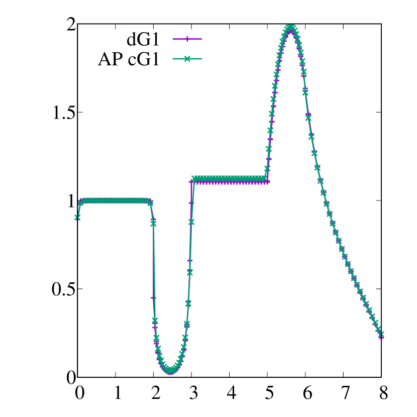
(a) Case 1, $\overline{\psi}_{h}$

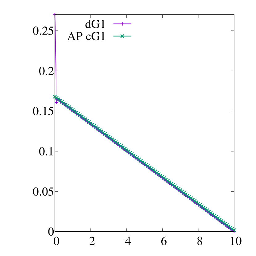
(b) Case 2, $\overline{\psi}_{h}$

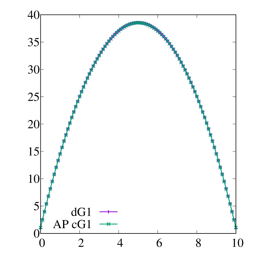
(c) Case 3, $\overline{\psi}_{h}$

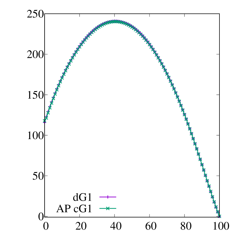
(d) Case 4, $\psi_{h,1}$

Figure 1: Comparison between the (first-order) positive, asymptotic preserving cG1 method and the (second-order) upwind dG1 method.

5.4 Boundary effects

We consider the problem (2.1) in the two-dimensional domain $D=(0,100)^{2}{\times}{\mathbb{R}}$ with uniform cross sections $\sigma_{t}({\bm{x}})=0.1$, $\sigma_{s}({\bm{x}})=0.0999$ and uniform source term $q({\bm{x}},{\bm{\Omega}})=1$ for all $({\bm{x}},{\bm{\Omega}})\in D{\times}{\mathcal{S}}$. The boundary condition is set to zero $\alpha({\bm{x}},{\bm{\Omega}})=0$ for all $({\bm{x}},{\bm{\Omega}})\in\partial D_{-}$. (This is the two-dimensional counterpart of the one-dimensional case 4 discussed in §5.3.) We use the $S_{6}$ quadrature for the discrete ordinates (24 directions in 2D). The approximation in space for the asymptotic preserving method is done on a non-uniform grid composed of $151294$ triangles with $76160$ grid points (i.e., $1\,829\,520$ dofs in total). The dG1 approximation is done with $64{\times}64$ cells, that is $16384$ space dofs (i.e., $393\,216$ dofs in total).

(a) $\overline{\psi}_{h}$, AP scheme

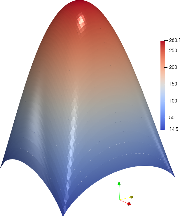
(b) $\overline{\psi}_{h}$, dG1 scheme

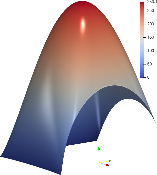
(c) $\psi_{h,1}$, AP scheme

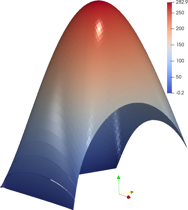
(d) $\psi_{h,1}$, dG1 scheme

Figure 2: Scalar $\overline{\psi}_{h}$ and angular flux $\psi_{h,1}$.

We show in Figure 2 the scalar flux and the angular flux corresponding to the first angle ${\bm{\Omega}}_{1}$. We have verified that the angular fluxes for the asymptotic preserving method are all non-negative, as expected, but the upwind dG1 approximation gives negative angular fluxes. In particular, we observe in Panel (2(d)) that the minimum value of the first angular flux of the dG1 approximation is equal to $-0.2$ (1 digit roundoff approximation.)

5.5 Reflection effects

We now consider the two-dimensional problem with reflection effects. The domain is $D=(0,1)^{2}{\times}{\mathbb{R}}$ with uniform cross sections $\sigma_{t}({\bm{x}})=100$, $\sigma_{s}({\bm{x}})=99$ if $x_{2}\geq 0.5$ (optically thick and diffusive zone), and $\sigma_{t}({\bm{x}})=\sigma_{s}({\bm{x}})=0$ if $x_{2}\leq 0.5$ (void). We use the $S_{6}$ quadrature. The left boundary is illuminated with intensity $1$ along the first direction of the quadrature ${\bm{\Omega}}_{1}:=(0.93802334,0.25134260,0.23861919)$ (eight digits truncation). The incoming flux is set to $0$ along the bottom boundary for ${\bm{\Omega}}_{1}$. For all the other angular fluxes we set $\psi_{h,k|\partial D_{-}}=0$, $k\in{\mathcal{L}}{\setminus}\{1\}$. The approximation in space for the asymptotic preserving method is done on a non-uniform grid composed of $151434$ triangles with $76230$ grid points (i.e., $1\,829\,520$ dofs in total). The dG1 computation is done with $256{\times}256$ cells to ascertain the accuracy of the solution since it is our reference; that makes $262144$ dofs for the space approximations (i.e., $6\,291\,456$ dofs in total).

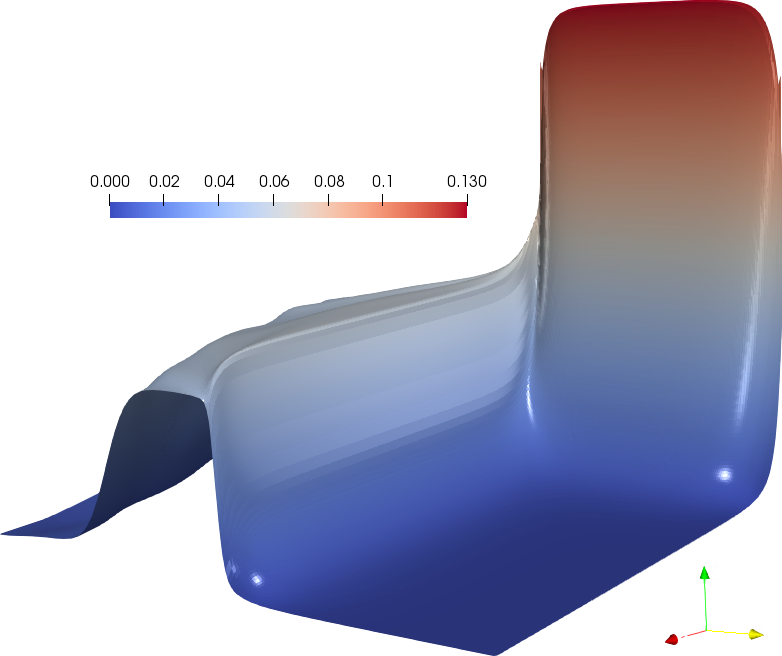
(a) $\overline{\psi}_{h}$, AP scheme

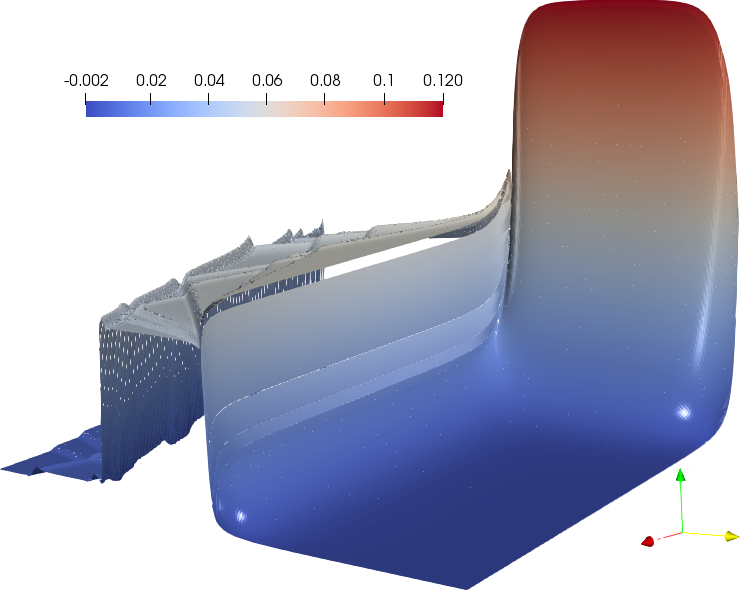
(b) $\overline{\psi}_{h}$, dG1 scheme

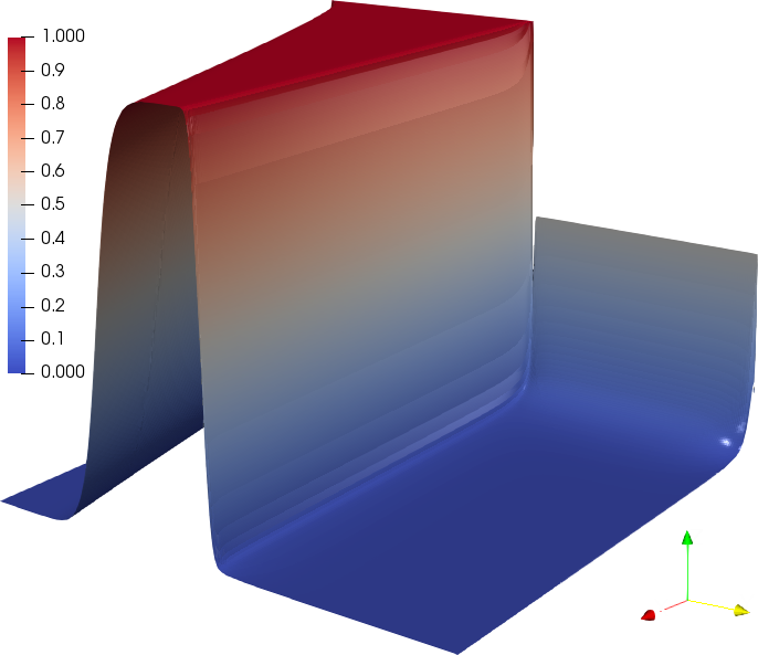
(c) $\psi_{h,1}$, AP scheme

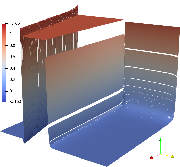
(d) $\psi_{h,1}$, dG1 scheme

Figure 3: Scalar $\overline{\psi}_{h}$ and angular flux $\psi_{h,1}$.

We show in Figure 3 the scalar flux and the angular flux corresponding to the first angle ${\bm{\Omega}}_{1}$. The angular fluxes for the asymptotic preserving method are all non-negative, but the upwind dG1 approximation gives negative values for the scalar flux and the angular fluxes. We observe that the minimum value of the dG1 scalar flux is approximately $-0.002$ (Panel (3(b))), and the minimum value is $-0.183$ for the first angular flux (Panel (3(d))). The dG1 approximation is obviously more accurate than the asymptotic preserving solution, but it experiences overshoots and undershoots at the interfaces between the two materials, whereas the positive asymptotic preserving solution does not.

6 Conclusions

We have introduced a (linear) positive asymptotic preserving method for the approximation of the one-group radiation transport equation (see (4.6)). The approximation in space is discretization agnostic: the approximation can be done with continuous or discontinuous finite elements (or finite volumes). The method is first-order accurate in space. This type of accuracy is coherent with Godunov’s theorem since the method is linear. The two key theoretical results of the paper are Theorem 4.4 and Theorem 4.9. We have illustrated the performance of the method with continuous finite elements. We have observed that the method converges with the rate ${\mathcal{O}}(h)$ in the $L^{2}$-norm on manufactured solutions. It converges with the rate ${\mathcal{O}}(h^{2})$ in the $L^{2}$-norm in the diffusion limit. The method has also been observed to be non-negative (in compliance with Theorem 4.9). It does not suffer from overshoots like the upwind dG1 approximation at the interfaces of optically thin and optically thick regions.

The present work is the first part of a ongoing project aiming at developing techniques that are high-order accurate, positivity-preserving, and robust in the diffusion limit. To reach higher-order accuracy the technique must be made nonlinear. This could be done by using smoothness indicators like in [10, §4.3], or by using limiting technique, or by enforcing positivity through inequality constraints (see e.g., Hauck and McClarren [12, §4]). Our progresses in this direction will be reported elsewhere.

References

• Adams and Larsen [2002] M. Adams and E. Larsen. Fast iterative methods for discrete-ordinates particle transport calculations. Progress in Nuclear Energy, 40(1):3–159, 2002.
• Adams [2001] M. L. Adams. Discontinuous finite element transport solutions in thick diffusive problems. Nuclear Science and Engineering, 137(3):298–333, 2001.
• Babuška and Suri [1992] I. Babuška and M. Suri. On locking and robustness in the finite element method. SIAM J. Numer. Anal., 29(5):1261–1293, 1992.
• Buet and Cordier [2004] C. Buet and S. Cordier. Asymptotic preserving scheme and numerical methods for radiative hydrodynamic models. C. R. Math. Acad. Sci. Paris, 338(12):951–956, 2004.
• Buet and Després [2006] C. Buet and B. Després. Asymptotic preserving and positive schemes for radiation hydrodynamics. J. Comput. Phys., 215(2):717–740, 2006.
• Buet et al. [2012] C. Buet, B. Després, and E. Franck. Design of asymptotic preserving finite volume schemes for the hyperbolic heat equation on unstructured meshes. Numer. Math., 122(2):227–278, 2012.
• Gosse and Toscani [2002] L. Gosse and G. Toscani. An asymptotic-preserving well-balanced scheme for the hyperbolic heat equations. C. R. Math. Acad. Sci. Paris, 334(4):337–342, 2002.
• Guermond and Kanschat [2010] J.-L. Guermond and G. Kanschat. Asymptotic analysis of upwind discontinuous Galerkin approximation of the radiative transport equation in the diffusive limit. SIAM J. Numer. Anal., 48(1):53–78, 2010.
• Guermond and Popov [2016] J.-L. Guermond and B. Popov. Invariant domains and first-order continuous finite element approximation for hyperbolic systems. SIAM J. Numer. Anal., 54(4):2466–2489, 2016.
• Guermond and Popov [2017] J.-L. Guermond and B. Popov. Invariant domains and second-order continuous finite element approximation for scalar conservation equations. SIAM J. Numer. Anal., 55(6):3120–3146, 2017.
• Guermond et al. [2019] J.-L. Guermond, B. Popov, and I. Tomas. Invariant domain preserving discretization-independent schemes and convex limiting for hyperbolic systems. Comput. Methods Appl. Mech. Engrg., 347:143–175, 2019.
• Hauck and McClarren [2010] C. Hauck and R. McClarren. Positive $P_{N}$ closures. SIAM J. Sci. Comput., 32(5):2603–2626, 2010.
• Jin [1999] S. Jin. Efficient asymptotic-preserving (AP) schemes for some multiscale kinetic equations. SIAM J. Sci. Comput., 21(2):441–454, 1999.
• Jin and Levermore [1996] S. Jin and C. D. Levermore. Numerical schemes for hyperbolic conservation laws with stiff relaxation terms. J. Comput. Phys., 126(2):449–467, 1996.
• Larsen [1983] E. W. Larsen. On numerical solutions of transport problems in the diffusion limit. Nuclear Science and Engineering, 83(1):90–99, 1983.
• Larsen and Morel [1989] E. W. Larsen and J. E. Morel. Asymptotic solutions of numerical transport problems in optically thick, diffusive regimes. II. J. Comput. Phys., 83(1):212–236, 1989.
• Larsen et al. [1987] E. W. Larsen, J. E. Morel, and W. F. Miller, Jr. Asymptotic solutions of numerical transport problems in optically thick, diffusive regimes. J. Comput. Phys., 69(2):283–324, 1987.
• Lesaint and Raviart [1974] P. Lesaint and P.-A. Raviart. On a finite element method for solving the neutron transport equation. In C. de Boor, editor, Mathematical aspects of finite elements in partial differential equations (Proc. Sympos., Math. Res. Center, Univ. Wisconsin, Madison, Wis., 1974), pages 89–123. Publication No. 33. Math. Res. Center, Univ. of Wisconsin-Madison, Academic Press, New York, 1974.
• Li and Wang [2017] Q. Li and L. Wang. Implicit asymptotic preserving method for linear transport equations. Commun. Comput. Phys., 22(1):157–181, 2017.
• Petra et al. [2014] C. G. Petra, O. Schenk, and M. Anitescu. Real-time stochastic optimization of complex energy systems on high-performance computers. Computing in Science Engineering, 16(5):32–42, Sep. 2014.
• Ragusa et al. [2012] J. C. Ragusa, J.-L. Guermond, and G. Kanschat. A robust $S_{N}$-DG-approximation for radiation transport in optically thick and diffusive regimes. J. Comput. Phys., 231(4):1947–1962, 2012.
• Reed and Hill [1973] W. Reed and T. Hill. Triangular mesh methods for the neutron transport equation. Technical Report LA-UR-73-479, Los Alamos Scientific Laboratory, Los Alamos, NM,, 1973.
• Wang and Ragusa [2010] Y. Wang and J. Ragusa. Diffusion synthetic acceleration for high-order discontinuous finite element ${S}_{n}$ transport schemes and application to locally refined unstructured meshes. Nuclear Science and Engineering, 166:145–166, 2010.
• Xu and Zikatanov [1999] J. Xu and L. Zikatanov. A monotone finite element scheme for convection-diffusion equations. Math. Comp., 68(228):1429–1446, 1999.