Neptune’s Latitudinal Variations as Viewed with ALMA

Abstract

We present spatially resolved millimeter maps of Neptune between 95 and 242 GHz taken with the Atacama Large Millimeter/submillimeter Array (ALMA) in $2016-2017$. The millimeter weighting functions peak between 1 and 10 bar on Neptune, lying in between the altitudes probed at visible/infrared and centimeter wavelengths. Thus, these observations provide important constraints on the atmospheric structure and dynamics of Neptune.

We identify seven well-resolved latitudinal bands of discrete brightness temperature variations, on the order of $0.5-3$K in all three observed ALMA spectral bands. We model Neptune’s brightness temperature using the radiative transfer code Radio-BEAR and compare how various H₂S, CH₄, and ortho/para H₂ abundance profiles can fit the observed temperature variations across the disk. We find that observed variations in brightness temperature with latitude can be explained by variations in the H₂S profile that range from sub- to super-saturations at altitudes above the 10-bar pressure level, while variations in CH₄ improve the quality of fit near the equator. At the south polar cap, our best fit model has a depleted deep atmospheric abundance of H₂S from 30 to only 1.5 times the protosolar value, while simultaneously depleting the CH₄ abundance. This pattern of enhancement and depletion of condensable species is consistent with a global circulation structure where enriched air rises at the mid-latitudes ($32^{\circ}-12^{\circ}$S) and north of the equator ($2^{\circ}-20^{\circ}$N), and dry air descends at the poles ($90^{\circ}-66^{\circ}$S) and just south of the equator ($12^{\circ}$S$-2^{\circ}$N). Our analysis finds more complex structure near the equator than accounted for in previous circulation models.

1 Introduction

Millimeter continuum observations of Neptune provide a valuable bridge between visible/infrared studies of the cloud tops and above ($P<1$ bar) and deeply probing centimeter maps ($10<P<40$ bar). Visible and near-infrared (NIR) imaging from Voyager, the Hubble Space Telescope (HST), and Keck have shown bright methane cloud activity at Neptune’s mid-latitudes and comparatively dark regions and/or hazes at the equator and poles (Limaye & Sromovsky, 1991; Sromovsky et al., 2001; Martin et al., 2012; Fitzpatrick et al., 2014; Tollefson et al., 2018). Mid-infrared (MIR) images and spectra have been used to obtain zonal-mean temperature profiles which show that the equator and south pole are warmer than the southern mid-latitudes in the upper troposphere and stratosphere (Conrath et al., 1991; Orton et al., 2007; Fletcher et al., 2014). Centimeter maps obtained with the Very Large Array (VLA) probe well below Neptune’s cloud deck and indicate the presence of dry (low-opacity) air at the south pole (e.g., Butler et al., 2012; de Pater et al., 2014). Taken together, observations of the deep troposphere and upper atmosphere are broadly consistent with a global circulation pattern where air enriched with trace gases rises at the mid-latitudes, adiabatically cools and condenses to form clouds, dries out, and descends at the poles and equator (Conrath et al., 1991; de Pater et al., 2014). Millimeter observations probe altitudes in between those seen in the above maps, $1<P<10$ bar, making such observations vital for bridging the pressures viewed in the visible/infrared and centimeter, and for improving our overall understanding of Neptune’s atmospheric structure and dynamics. In particular, millimeter continuum observations are sensitive to variations in composition, including variations in trace condensable species such as H₂S and CH₄. Like the centimeter, millimeter observed variations in these trace gases reflect atmospheric motions; depleted, low-opacity regions (enriched, high-opacity) are consistent with downwelling (upwelling) air.

The opacity of Neptune’s continuum at millimeter observations is dominated by collision-induced absorption of H₂ (CIA) with hydrogen, helium, and methane. Trace gases, such as H₂S, PH₃, and NH₃ also contribute to the overall opacity. Since millimeter observations of these gases probe Neptune’s troposphere between 1 and 10 bar, individual lines are highly pressure-broadened, appearing as broad ‘continuum’ bands in the millimeter spectrum. As a result, it is difficult to differentiate between these opacity sources since clear line features cannot be detected.

On previous millimeter maps, Neptune’s disk was spatially resolved and regions of enhanced or diminished brightness temperatures could be distinguished. Using the Combined Array for Research in Millimeter-wave Astronomy (CARMA), Luszcz-Cook et al. (2013b) imaged Neptune in the far wings of the CO ($2-1$) line (230.538 GHz). In their longitudinally-averaged maps, they found brightness temperatures increased by $2-3$ K from $40^{\circ}$N to the south pole. Since their observations were taken far ($\sim 5$ GHz) from the CO ($2-1$) line center, this emission is primarily from sources forming the ’quasi-continuum’. Assuming an adiabat in the troposphere, the authors showed that variations in the brightness temperature at the south pole could be explained by a 30% decrease in opacity at $P>1$ bar. If variations in opacity would occur at altitudes only below 4 bar, the opacity needed to be decreased by a factor of 50. Hence, brightness variations at a particular wavelength are coupled to the pressure at which the opacity changes, itself dependent on the opacity source. Luszcz-Cook et al. (2013b) could explain the latitudinal variations in brightness temperature as latitudinal gradients in any or all of: H₂S, CH₄, and/or ortho/para H₂. However, due to their limited wavelength coverage, they were unable to disentangle the true contribution to the brightness from each candidate source.

In this paper, we present millimeter maps of Neptune taken with the Atacama Large Millimeter/Submillimeter Array (ALMA). ALMA provides the wavelength coverage, sensitivity, and resolution needed to constrain Neptune’s opacity sources accurately across the disk. In Section 2, we present ALMA observations taken in three bands over the millimeter wavelength range ($1-3$ mm). The observed brightness temperature distribution is compared to model maps produced with the radiative-transfer code Radio-BEAR, described in Section 3. We generate a model for the latitudinally-varying H₂S and CH₄ abundance profiles that agree with the observations in each band in Section 4. In Section 5, we compare these results to other profiles of Neptune’s trace gases and summarize how our findings impact our understanding of the dynamics and evolution of Neptune’s upper atmosphere.

2 Observations

2.1 Data

We observed Neptune with ALMA, which is an interferometer located in the Atacama desert in northern Chile. A total of 66 high-precision antennas form the array: fifty-four 12m and twelve 7m. The arrangement of these antennas defines the angular resolution and maximum resolvable angular scale of the data. The tightest packed configuration, where the antennas are up to 150 m apart, allow large, faint objects to be observed. Extended arrangements, where the antennas are 16 km apart, provide a more detailed look. Our Neptune observations were taken between $2016-2017$ in Bands 3, 4, and 6, between $95-250$ GHz (1–3 mm). For each band, we selected the antenna configuration which allowed us to resolve Neptune and simultaneously see Neptune’s entire (2.3” diameter) disk. A typical resolution was 0.3” using $\sim 40$ 12-m antennas. We observed in four spectral windows in continuum mode covering Neptune’s continuum spectra within each band. Table 1 summarizes the observations while Table 2 outlines the correlator and spectral setup.

Table 1: Summary of observations.

ALMA Band	Configuration	UT Date	Flux Calibrator	Bandpass Calibrator	T${}_{\text{Source}}^{a}$
Band 3	C40-8	2017-07-27	J0006-0623	J2246-1206	726
Band 4	C40-7	2016-10-07	J2258-2758	J2246-1206	1701
Band 6	C40-7	2016-10-24	J2258-2758	J2246-1206	1032

^a Total science time on Neptune, in seconds

Table 2: Summary of correlator setup, spectral windows, and synthesized beams.

ALMA Band	Center Frequency	Center Wavelength	Channel Width	Total Bandwidtha	Beam Size	Position Angleb
	(GHz)	(mm)	(MHz)	(MHz)	(arcsec2)	(degrees)
Band 3	95.012 96.970 107.000 109.000	3.155 3.092 2.802 2.750	15.625	2000	0.45”$\times$0.33” 0.44”$\times$0.33” 0.40”$\times$0.30” 0.39”$\times$0.29”	$281.5^{\circ}$ $282.1^{\circ}$ $282.9^{\circ}$ $282.9^{\circ}$
Band 4	135.986 137.924 147.986 149.986	2.205 2.174 2.026 1.999	15.625	2000	0.38”$\times$0.28” 0.38”$\times$0.28” 0.35”$\times$0.26” 0.35”$\times$0.26”	$23.0^{\circ}$ $24.8^{\circ}$ $22.7^{\circ}$ $24.3^{\circ}$
Band 6	223.982 225.982 239.981 241.981	1.338 1.327 1.249 1.239	15.625	2000	0.31”$\times$0.25” 0.32”$\times$0.24” 0.30”$\times$0.23” 0.29”$\times$0.23”	$64.3^{\circ}$ $61.8^{\circ}$ $64.0^{\circ}$ $63.6^{\circ}$

^a Each spectral window has the same total bandwidth, consisting of 128 channels with the same channel width.
^b Defined as north through east.

2.2 Calibration and Imaging

The obtained visibility data were reduced and calibrated in the Common Astronomical Software Application (CASA) version 5.1. We applied the standard ALMA pipeline to perform flagging (bad edge channels, shadowed antennas, and poor quality data), bandpass and flux calibration, and gain-time solutions. Table 1 lists our calibrator sources. Finally, we applied three iterations of self calibration on our Neptune data to remove short-term phase variability caused by fast atmospheric fluctuations (Brogan et al., 2018). The first iteration used the entire observation range while the second and third used 350-second and 60-second intervals.

The multi-frequency synthesis mode in CASA tclean was used to transform the visibility data into image maps. We used natural weighting and restricted clean to a circular mask that is roughly the size of Neptune’s diameter plus twice the beam size. The natural weighting scheme gives equal weight to all baseline samples while the uniform weighting scheme gives equal weight to each spatial frequency. Since there are ‘naturally’ more short baselines than long baselines, natural weighting preserves the peak sensitivity while uniform weighting reduces the peak sensitivity as the short baselines have been weighted less. In our testing, we found that uniform and intermediate weightings produced artificial speckles on the disk and large scale structures in the sky. Natural weighting limits these artifacts since the sensitivity is highest, but sacrifices some angular resolution since the long-baselines are under-weighted relative to the uniform scheme. Despite this, we still resolve roughly one-seventh of Neptune’s disk. We also subtracted a limb-darkened model from the data to speed up the deconvolution process and reduce imaging artifacts. The number of clean iterations varied from 1000-2000, stopping once the noise within the planetary disk reached the noise in the sky.

Our resulting maps are 512$\times$512 pixels² with a cell size of 0.02”. This cell size follows a common rule-of-thumb, which is to make the cell size roughly 1/10 the size of the synthesized beam. The planetary disk appears elliptically elongated due to convolution with the synthesized beam. This beam resembles a Gaussian with full-width at half maxima and position angles given in Table 2.

2.3 Error estimation

The error in our maps is calculated by averaging over four regions of the sky with boxes equal to the diameter of Neptune and taking the root-mean-square (RMS). RMS values range from $0.1-0.6$K. Table 3 lists our estimated errors in each band. This RMS does not include systematic effects, such as errors in the bandpass or flux calibration. The ALMA Calibrator Source Catalogue lists errors in the calibrator’s flux estimate being about 5$\%$ or less in each band so we use this as an estimate for the absolute error in our disk-averaged temperature data (Section 5.1).

Table 3: Summary of observed and modeled millimeter disk-averaged brightness temperatures.

Center Frequency (GHz)	Observed Flux Densitya (Jy)	Observed T${}_{\text{b}}^{a}$ (K)	Nominal T${}_{\text{b}}^{b}$ (K)	Noisec (K)	Factord
95.012	$3.4\pm 0.2$	$126.6\pm 6.3$	119.9	0.1	0.945
96.970	$3.5\pm 0.2$	$126.0\pm 6.3$	119.4	0.1	0.950
107.000	$4.1\pm 0.2$	$120.5\pm 6.0$	116.7	0.2	0.975
109.000	$4.1\pm 0.2$	$118.8\pm 6.0$	116.1	0.3	0.975
135.986	$5.9\pm 0.3$	$108.5\pm 5.4$	109.0	0.3	1.010
137.924	$6.1\pm 0.3$	$108.0\pm 5.4$	108.5	0.2	1.010
147.986	$6.7\pm 0.3$	$104.3\pm 5.2$	105.7	0.2	1.020
149.986	$6.8\pm 0.3$	$104.5\pm 5.2$	105.1	0.3	1.025
223.982	$13.3\pm 0.7$	$93.4\pm 4.7$	94.8	0.4	1.020
225.982	$13.5\pm 0.7$	$93.0\pm 4.7$	94.7	0.4	1.025
239.981	$15.1\pm 0.8$	$93.1\pm 4.7$	93.4	0.6	1.010
241.981	$15.3\pm 0.8$	$92.8\pm 4.6$	93.2	0.6	1.010

^a The listed errors are the absolute errors, estimated at $5\%$ from the calibrators.
^b The nominal model assumes a dry adiabat with trace gases enhanced by 30$\times$ the protosolar value.
^c Random errors defined as the RMS on the sky.
^d This factor is used to scale the observed brightness temperature to match the nominal model to within the estimated noise.

3 Models

2D model maps of Neptune’s disk were created using our radiative transfer (RT) code Radio-BEAR described in de Pater et al. (2019). Given an atmospheric composition and thermal structure (described below), we calculate the RT-derived brightness temperatures of the planet on each location on the planet.

Radio-BEAR assumes that the atmosphere is in local thermodynamic equilibrium, where the temperature is calculated from deep in the atmosphere upwards assuming a dry or wet adiabat such that the temperature at 1 bar matches 71.5 K, that derived by Voyager radio occultation measurements (Lindal, 1992). At altitudes above 1 bar, we use the temperature profile from Fletcher et al. (2010). The temperature, pressure, and altitudes are related to each other through hydrostatic equilibrium. In all of our latitude-varying models (Sections 4.2 and 4.3), we assume that the temperature-pressure profile follows a dry adiabat in the troposphere. Cases of a wet adiabat are presented in the context of the disk-averaged brightness temperature in section 4.1. Our models also allow the abundance profiles of H₂S, CH₄ and ortho/para H₂ to vary, as discussed below.

Neptune’s trace gases H₂S, CH₄, H₂O, and NH₃ in the deep atmosphere are assumed to be enhanced by $30\times$ their protosolar values in our nominal model, apart from ammonia gas as 30$\times$ protosolar values for NH₃ are inconsistent with previous microwave disk-averaged temperatures (de Pater & Massie, 1985; de Pater et al., 2014). At higher altitudes, these gases follow the saturated vapor pressure curve with 100$\%$ relative humidity. Clouds expected to form under thermochemical equilibrium on Neptune include: an aqueous ammonia solution (H₂O-NH₃-H₂S) topped with water ice, ammonium-hydrosulfide (NH₄SH), and H₂S- and CH₄-ice (Weidenschilling & Lewis, 1973). To form the NH₄SH cloud, H₂S and NH₃ are reduced in equal molar quantities until the product of their partial pressures reaches the equilibrium constant of the reaction forming NH₄SH. Once equilibrium is reached, only H₂S will remain to form clouds since there is practically no NH₃ gas remaining above the NH₄SH cloud. A tentative detection of H₂S spectral features near 1.58 $\mu$m in Neptune’s troposphere implies that the deep bulk S/N ratio is greater than one (Irwin et al., 2019). The cloud density might affect microwave measurements (de Pater et al., 1991; de Pater & Mitchell, 1993). However, little is known about the cloud density on Neptune and the millimeter weighting functions peak at altitudes above the aqueous and ammonium-hydrosulfide clouds (see Fig. 1). Clouds have also been shown to not affect the microwave opacity on Jupiter (de Pater et al., 2019). Therefore, we ignore the effect of cloud opacity and focus on the gas opacity in our models.

The gas opacity of Neptune’s millimeter spectrum is dominated by H₂S and the collision-induced absorption (CIA) of H₂ (we include: H₂-H₂, H₂-He, H₂-CH₄). NH₃ and H₂O affect the spectra at wavelengths longer than 10 cm; NH₃ would have a larger impact at millimeter wavelengths if its abundance within Neptune were larger (see Fig. 4 of Luszcz-Cook & de Pater (2013a)). The effect of PH₃ in the millimeter is most prominent at the ($1-0$) absorption line at 266.9 GHz. The width of this line is $\sim$ 20 GHz due to pressure broadening, meaning the wings of this absorption feature will have a small effect on the highest frequency data. However, this effect is well within the estimated noise of the maps so we do not add this gas in our models.

The ortho/para H₂ fraction also influences Neptune’s millimeter brightness temperature, by modifying both the adiabatic lapse rate and the gas opacity (Trafton, 1967; Wallace, 1980; de Pater & Massie, 1985; de Pater & Mitchell, 1993). The ratio of ortho to para hydrogen in equilibrium depends on temperature; however, fast vertical mixing could bring the ratio of ortho and para states of hydrogen away from equilibrium and towards a “normal” ratio of 3 parts ortho to 1 part para. In this paper, we assume “intermediate” H₂ proposed by Trafton (1967) and used by e.g., Luszcz-Cook et al. (2013b): the ortho and para states of hydrogen (which define the CIA opacities) are set to the equilibrium value at the local temperature, while the specific heat is set to that of ’normal’ hydrogen. For further explanation of intermediate hydrogen, see e.g., Massie & Hunten (1982). Luszcz-Cook et al. (2013b) find that assuming a normal hydrogen fraction rather than equilibrium fraction significantly increases the opacity and lowers the brightness temperature by $5-6$K in their 1.2-mm model maps.

We generate 2D model maps of Neptune as follows: at the center frequencies of each spectral window, we calculate the RT-derived brightness temperatures of the planet on 9455 points on the disk and interpolate between these points to obtain the same resolution as our CASA imaged maps (0.02”). We then convolve each RT-map with an elliptical gaussian model of the synthesized beam. Our nominal model can be summarized as follows: 1) Neptune’s trace gases are enhanced to 30$\times$ their protosolar value, except NH₃ which is $1\times$ protosolar; 2) ‘intermediate’ ortho/para H₂ (i.e., equilibrium ortho/para H₂; specific heat close to that of normal H₂); 3) the temperature-pressure profile follows a dry adiabat in the troposphere. Figure 2 plots the temperature-pressure and abundance profiles for the nominal model. In the following section, we compare these beam-convolved model maps to the observed disk-averaged brightness temperatures and latitudinal brightness variations.

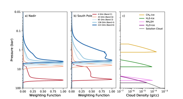
Figure 1: Normalized weighting functions at: a) nadir and b) the south pole, compared to the expected clouds expected to form on Neptune (c). The weighting functions at nadir and the south pole are both computed using the nominal abundance profile depicted in Figure 2. Weighting functions are shown for representative frequencies in each ALMA band: 95 GHz (3.155 mm, Band 3), 136 GHz (2.205 mm, Band 4), and 224 GHz (1.338 mm, Band 6), as well as selected VLA frequencies: 4 and 43 GHz (6.2 cm and 0.7 cm, respectively). Note that the VLA frequencies probe significantly deeper into Neptune’s atmosphere than the ALMA frequencies. The rightmost plot shows the density of different clouds expect to form on Neptune under thermochemical equilibrium.

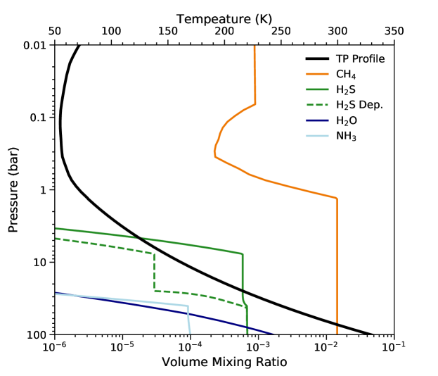
Figure 2: Temperature and abundance profiles of trace gases whose deep atmospheric abundances are enhanced by 30$\times$ their protosolar value, apart from NH₃ which is $1\times$ (solid lines). In the troposphere, the temperature follows a dry adiabat. These profiles define the nominal model. The dashed line is the H₂S depleted profile that that best fits Neptune’s south pole from 2003 VLA data (de Pater et al., 2014).

4 Results

In the following subsections, we investigate the distribution of Neptune’s observed brightness temperature. First, we look at the disk-averaged brightness temperature and compute a variety of RT models using dry and wet adiabats and different enhancements of the deep abundance of trace gases. From these results, we present our nominal model (the same as that described at the end of Section 3), which fits both our ALMA and 2003 VLA disk-averaged temperatures simultaneously. Second, we subtract our nominal model from the data to produce residual maps. These maps show seven distinct latitudinal bands across Neptune’s disk. In the final subsections, we find abundance profiles of H₂S, CH₄, and ortho/para H₂ which fit the observed brightness variations in each latitudinal band. As an example of how we do this, we first look at Neptune’s south polar cap, where previous VLA studies constrained the deep abundance of H₂S. This provides a good litmus test for our model and fitting routine. We then move on to the rest of Neptune’s disk and show that we can fit the observed brightness temperature distribution at all latitude bands by varying the abundances of the aforementioned species.

4.1 Disk-Averaged Brightness Temperatures

We calculate Neptune’s disk-averaged brightness temperature from the ALMA data in two ways. First, we sum the flux density contained within the planetary disk convolved with the model beam. Second, we fit the u-v short-spacing amplitude with a Bessel function and obtain an estimate of the zero-spacing flux density. Both results agree to well within the absolute calibration errors. We report the average of these two methods in Table 3. Since Neptune blocks the cosmic microwave background (CMB), its true brightness temperature is higher than observed in the radio. In all of our millimeter observations, we correct for the CMB by following the procedure laid out in Appendix A of de Pater et al. (2014).

Figure 3 plots our observed radio disk-averaged brightness temperatures on top of RT model spectra. In this plot, we show the effect of varying the deep abundance enhancement of trace gases (H₂S, CH₄, H₂O, and NH₃) relative to their protosolar values and consider both wet and dry lapse rates. We find that the nominal model: 30$\times$ enhancement with a dry lapse rate, agrees very well with both the ALMA millimeter and the 2003 VLA centimeter data from de Pater et al. (2014). Models with temperatures following wet lapse rates are too cold relative to these data. We acknowledge, though, the following shortcomings in our models. First, these models are highly degenerate. Gas abundances are seldom at 100$\%$ humidity and so a profile with a wet adiabat where the gases are sub-saturated may result in high enough brightness temperatures to match the data. Second, our models do not account for the cooling (heating) of the atmosphere from adiabatic expansion (compression) at latitudes where the air is rising (sinking). Finally, apart from the dry and wet adiabat, we do not consider latitudinal variations in temperature. Conrath et al. (1998) and Orton et al. (2007) see $2-3$ K latitudinal temperature variations between $50-100$ mbar. These temperature variations are similar in strength to those we see in our residual maps (Fig. 4), particularly in Band 6. Luszcz-Cook et al. (2013b) created temperature profiles matching the $2-3$ K variations described in Conrath et al. (1998) and Orton et al. (2007) at altitudes above 1 bar. These temperature-varying models reduced the overall $\chi^{2}$ in their fit to 1.2 mm continuum data. However, we expect similar profiles to have only a modest effect in Band 6, where the contribution functions peak at the highest altitudes (but still below 1 bar, see Fig. 1), and little effect in Bands 3 and 4, which probe pressures much higher than where temperature variations are seen in the infrared. Below 1 bar, the temperature profile should strictly follow an adiabat, regardless of latitude. In summary, while we do not consider temperature variations in our analysis, we do not expect them to be the primary cause of the observed brightness temperature distribution.

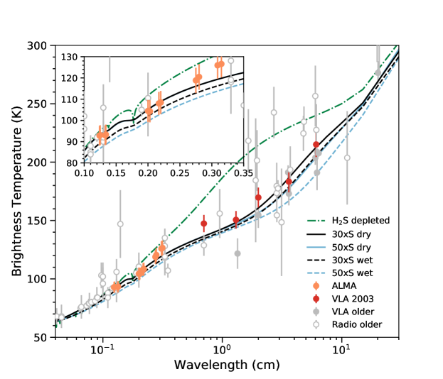
Figure 3: Disk-averaged brightness temperatures of Neptune. The ALMA data are plotted as orange points, with 5% absolute errors estimated from the calibrators. In addition, VLA 2003 data are plotted in red (de Pater et al., 2014), along with older VLA data in gray (de Pater et al., 1991) and older single dish radio data in open circles (de Pater & Richmond, 1989). Overplotted are model spectra which vary the deep abundance of H₂S, CH₄, and H₂O (30$\times$ and 50$\times$ their protosolar values in black and light blue respectively), and compare dry and wet lapse rates (solid and dashed lines, respectively). A model for Neptune’s south polar hot spot which depletes H₂S above 43 bar is also shown in the dot-dash green line (de Pater et al., 2014).

4.2 Latitudinal Brightness Temperature Variations

In Figure 4, we show residual maps of Neptune in the first spectral window of each ALMA band. Since the absolute calibration is imperfect, each map is scaled by a factor such that the observed disk-averaged temperature matches the nominal model (see Table 3). As a result, our main assumption in this analysis is that Neptune’s disk-average matches the nominal model. Deviations from this model result in the latitudinal structure evident in the residuals. This structure is due to changes in the brightness temperature that we assume to be due to variations in the opacity. The dark areas at the southern mid-latitudes and in the northern equatorial region are interpreted as probing higher, colder altitudes due to enhancements in absorbers. Conversely, the south pole appears bright in the radio due to opacity depletions, allowing the deeper, warmer layers to be probed.

Planetary coordinates are computed for each pixel on the disk using ephemeris data from JPL Horizons, with the center pixel equaling the sub-observer latitude and longitude. Latitudes are reported in planetographic coordinates. We identify seven bands on Neptune that correspond to discrete changes in the temperature structure: 90^∘S$-66^{\circ}$S, 66^∘S$-55^{\circ}$S, 55^∘S$-32^{\circ}$S, 32^∘S$-12^{\circ}$S, 12^∘S$-2^{\circ}$N, 2^∘N$-20^{\circ}$N, northward of 20^∘N. Each latitude bin is well-resolved, covering at least the total area of the ALMA beam, and is in planetographic coordinates. In Figure 5, we plot the average temperature difference between the data and nominal model per spectral window and band. Differences that are twice the RMS noise reported in Table 3 are significant.

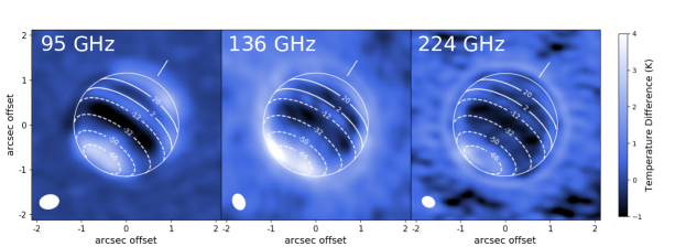
Figure 4: ALMA residual maps where the beam-convolved nominal model has been subtracted from the data. Contour lines delineate the latitude transitions between bands. Dark bands represent cold brightness temperatures relative to the model, while bright bands are warmer than the model. The FWHM of the beam is indicated in white in the bottom left of each map.

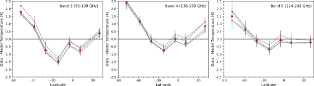
Figure 5: Residual temperatures comparing the data to the beam-convolved nominal model versus latitude (Band 3 left, Band 4 middle, Band 6 right). Points are plotted at the central latitude in the seven identified bins. The four gray dashed lines are the residual temperatures for each of the four spectral windows in a band. Red triangles are the average residual over each spectral window. The residuals in each latitude bin are calculated by averaging over each pixel within 60^∘ of the sub-observer longitude. Error bars are the image noise divided by the square-root of the number of ALMA beams that fit into the corresponding bin.

4.3 Neptune’s South Polar Cap

The ALMA residual maps show clear warming on Neptune at latitudes southward of -66^∘. This region is Neptune’s south polar cap and has been detected as a hot spot in the radio (Butler et al., 2012; Luszcz-Cook et al., 2013b; de Pater et al., 2014) and in the mid-infrared (Hammel et al., 2007; Orton et al., 2007). de Pater et al. (2014) found a best fit to their VLA data to the hot spot by defining a ‘plateau’ of constant low opacity from 66^∘S to the south pole, depleting H₂S to 1.5$\times$ the protosolar value (or 5$\%$ their nominal 50$\times$ model) above 43 bar (i.e., above the NH₄SH cloud). The deep CH₄ abundance is also depleted to 1.5$\times$ the protosolar value in their model (equivalently, a 0.072$\%$ volume mixing ratio), but itself is not a source of opacity at cm-wavelengths and so this study did not attempt to constrain the south pole CH₄ content (although methane does affect the adiabat and opacity due to CIA). Luszcz-Cook et al. (2013b) found that the high southern latitudes in their CARMA 1.3-mm map were consistent with the VLA model. In Figure 2, we show this depleted profile and in Figure 6 we compare the bin-averaged residual brightness temperatures for the ALMA observations and the de Pater VLA depleted model. We find good agreement in Band 6, which covers the frequency of the CARMA map, however the model is too bright at lower frequencies. Luszcz-Cook et al. (2013b) found that the high southern latitudes in their CARMA data could be matched if CH₄ were depleted to 0.55$\%$, while keeping H₂S at the nominal value. A comparison of our data with this CH₄ depleted model is also shown in Figure 6. Once again, the Band 6 data agree with the 1.3-mm map of Neptune presented in Luszcz-Cook et al. (2013b) to within their estimated uncertainties. However, the model is too cold to match the new low frequency data.

A better fit at low frequencies is obtained by setting the deep atmospheric CH₄ abundance to 0.55$\%$ and by depleting H₂S to 1.5$\times$ protosolar from 43 bar up to the saturated vapor pressure curve. The H₂S abundance follows the saturated vapor pressure curve below 4.5 bar; for $P<4.5$ bar, H₂S is subsaturated down to $5\%$ of the saturated vapor curve. This adjusted profile is plotted in Figure 7 and the temperature residuals are shown in Figure 6. We emphasize that some subsaturation is needed in order to fit the data well. Since the millimeter is most sensitive to the pressures where H₂S saturation occurs, all models in which H₂S profiles follow the saturated vapor pressure curve appear indistinguishable in terms of their contributions to the overall opacity and all under-predict the brightness temperatures in this region. Therefore, even models significantly depleting the deep abundance of H₂S will have temperatures that are too cold at the south pole and will resemble the residuals in Figure 5.

With this new depleted model for Neptune’s south polar hot spot, we can fit the VLA, CARMA, and ALMA data simultaneously. This is because the VLA cm-data probe pressures deeper than our alterations at the H₂S saturation curve and we have not changed the deep H₂S abundance estimated from de Pater et al. (2014) nor the deep CH₄ abundance determined by Luszcz-Cook et al. (2013b). The CARMA maps have larger uncertainties ($2-4$ K) than our maps presented here, and so depleting both H₂S and CH₄ is consistent with those data.

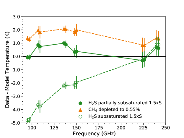
Figure 6: Residuals of the south polar data minus each of three different models, as described in Section 4.3. The dashed green line represents the residuals for the data compared with the model assuming H₂S subsaturation to $5\%$ of its nominal value, as suggested by the VLA cm data in de Pater et al. (2014). The orange dashed line and orange triangles are residuals to the south pole region in a model which only depletes CH₄ to 0.55$\%$, holding the other trace gases to their nominal values. The solid green line represents the residuals for the data compared with a model in which H₂S is partially subsaturated. This model depletes H₂S to 1.5$\times$S above 43 bar before following the saturation vapor pressure curve up to 4.5 bar and becoming subsaturated at higher altitudes (see Figure 7 for a plot of this profile). Simultaneously, CH₄ is depleted to 0.55$\%$ in the deep atmosphere. This is our preferred model and is consistent with the observations of de Pater et al. (2014) and Luszcz-Cook et al. (2013b).

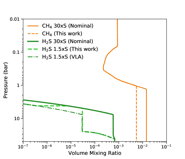
Figure 7: H₂S (green) and CH₄ (orange) abundance profiles. Models depleting one or both of these gases are used to explain radio brightness enhancements at Neptune’s South Pole. The 30$\times$S nominal profiles are shown as solid lines. The H₂S model fitting VLA measurements depletes H₂S down to $5\%$ (1.5$\times$S) of the nominal profile at $P<43$ bar; this profile is plotted as a dot-dash green line (de Pater et al., 2014). Our models for the H₂S and CH₄ profile, which simultaneously fits the ALMA, CARMA, and VLA measurements, are plotted as dashed lines. Note that in our H${}_{2}S$ profile, H₂S partially follows the saturation pressure curve, and follows the subsaturated profile of de Pater et al., 2014 higher than 4.5 bar.

4.4 Constraining Neptune’s Variations with Latitude

From Figures 4 and 5, it is clear that the magnitude of temperature variations across Neptune’s disk varies with wavelength. In the millimeter, these variations are caused by altering the abundance of trace gases: H₂S and CH₄, or changing the fraction of ortho/para H₂. Figure 8 compares the millimeter-spectrum of the nominal model to that of models depleted in trace gases. These plots show that the spectral shape varies with both wavelength and composition. Models where the H₂S profile follows the saturated vapor pressure curve differ little from the nominal model, no matter the abundance alterations in the deep troposphere. This is because the ALMA bands probe altitudes above 10 bar, where H₂S saturation begins, meaning changes in the constant deep abundance profile are undetected. On the other hand, models which subsaturate H₂S significantly increase the brightness temperature at short frequencies. The Band 6 (high frequencies) contribution functions peak between $1-5$ bar while Band 3 (low frequencies) probes between $5-10$ bar, altitudes close to where H₂S begins saturation. Thus, subsaturating H₂S results in a larger loss of opacity at low frequencies than the frequencies which probe higher altitudes, meaning low frequencies are able to probe deeper, warmer layers. In contrast, depleting CH₄ results in uniform increases across the millimeter. Substituting normal hydrogen for equilibrium hydrogen decreases the brightness temperature by 4K in Band 6 and less than 2K in Band 3. These differences with wavelength enable us to disentangle the effect of each constituent on the observed brightness temperatures in each spectral band.

In the following subsections, we present models where we vary a single constituent: H₂S, CH₄, or ortho/para H₂, while holding the others at their nominal value. We find the profiles which best match the data in each latitude bin for a single band. Then, we compare how well this matches the data in the other spectral bands. This gives a sense of how important the varied constituent is in producing model temperatures for each observation. Following this procedure, we present our best model fits to all three spectral bands where every parameter is allowed to vary. Table 4 describes how the constituent profiles change over all latitude and models.

The significance of our results within a particular latitude bin is computed with the reduced $\chi^{2}$:

$$\chi^{2}=\frac{1}{M-N}\sum_{m=0}^{M-1}\frac{\delta T_{m}^{2}}{\sigma_{m}^{2}},$$ (1)

where $\delta T_{m}$ is the difference between the data and model brightness temperature at each spectral window $m$, $\sigma_{m}$ is the image noise (see Table 3) divided by the square root of the number of beams that fit within the particular latitude bin. $M-N$ is the number of degrees of freedom in the model. We calculate the probability $p$ that this value of the reduced $\chi^{2}$, or a larger one, could arise by chance given $M-N$. We take the number of degrees of freedom to be eight: twelve spectral windows ($M$) minus four free parameters ($N$): the deep abundances of H₂S and CH₄, the ortho/para H₂ fraction, and the scaling factor assumption. For eight degrees of freedom, $p<0.05$ when the reduced $\chi^{2}>15.5$. Therefore, models with reduced $\chi^{2}>15.5$ are unlikely to occur due to random chance and are inconsistent with the observations. Table 5 summarizes the various fits to the data across each latitude range.

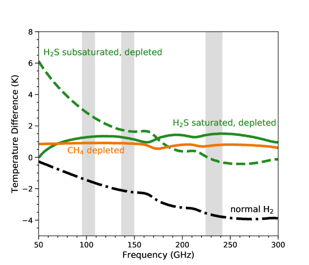
Figure 8: A comparison of models of Neptune’s spectrum to gauge how different opacity sources affect the brightness temperature across millimeter wavelengths. Plotted is the disk-averaged brightness temperatures for various models with the nominal model subtracted. The orange model depletes CH₄ to 15$\times$ the protosolar value (0.72$\%$) below saturation and the follows saturated vapor pressure curve above (as in the dashed-orange line in Fig. 7). The solid green model depletes H₂S to 15$\times$ the protosolar value (3.52E-4 mixing ratio) in the deep atmosphere, but follows the saturation curve. The dashed green model depletes H₂S similarly, but subsaturates H₂S by the same fraction (similar to the dashed green profile in Figure 2). The black dot-dash model substitutes opacity by normal hydrogen for equilibrium hydrogen. Gray rectangles indicate the ALMA bands (Bands 3, 4, and 6 left-to-right).

4.4.1 Varying H₂S

We first consider variations in H₂S that best match the Band 3 latitude variations. For each latitude band other than the south pole, we produce a grid of models in which the H₂S mixing ratio above 43 bar (the NH₄SH cloud) is set from $5-30\times$ solar in 5$\times$S steps. The profile then follows the saturation curve up to 4.5 bar, and is either depleted above 4.5 bar or supersaturated to a higher altitude. We choose 4.5 bar as this transition pressure as this matches the data at the south pole best. For supersaturated models, the H₂S abundance is set to the constant deep atmospheric value until $5-7$ bar, testing a grid of models in 0.25 bar steps. At altitudes above 3 bar (the high-altitude limit of H₂S cloud formation), the H₂S profile follows the saturation curve. At pressures in between 3 bar and $5-7$ bar, the abundance is assumed to be linear in log-log space. For the south pole, we do not produce new model fits but continue to use the model from Section 4.3, which is depleted to a much higher depth to be consistent with VLA observations. The deep CH₄ abundance is held to its nominal value of 1.44$\%$ ($30\times$ S) and equilibrium H₂ is assumed. Figure 9 plots example H₂S profiles used in these fits.

From the residuals plotted in Figure 10, there is general good agreement between the data and model in each band, apart from 12^∘S$-2^{\circ}$N where the model in Bands 4 and 6 is too warm compared to the data. This suggests the need to enhance CH₄ or add normal H₂ in this area.

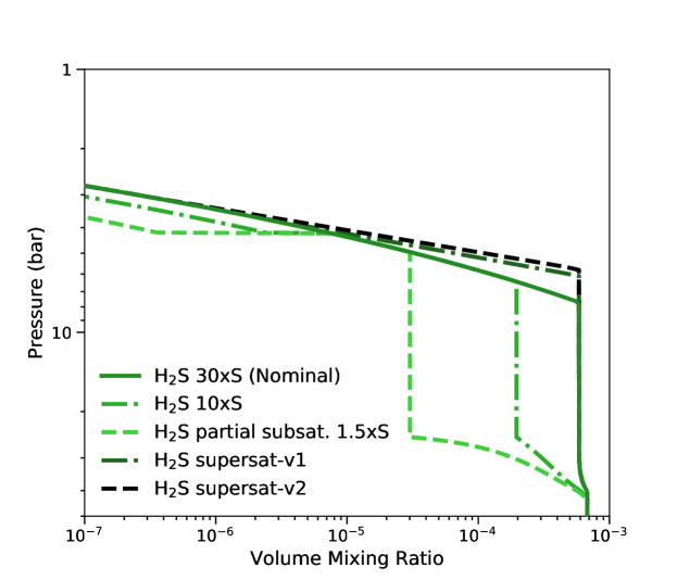
Figure 9: Examples of H₂S abundance profiles used to best fit the ALMA data. The light green dashed line and solid green line are the same profiles as depicted in Fig. 7. The dark green and black dashed and dot-dashed lines are supersaturated profiles (abbreviated supersat-v1 and supersat-v2).

Figure 10: Residual temperatures comparing the data to the beam-convolved nominal model versus latitude, as in Fig. 5, allowing H₂S (only) to vary with latitude to best-match the Band 3 data.

4.4.2 Varying CH₄

In order to determine if variations in CH₄ may effect the brightness temperature, we find CH₄ profiles which fit Band 6 to within the error bars of the average residual of the four spectral windows. The H₂S abundance is held at the nominal 30$\times$S profile and equilibrium H₂ is assumed. CH₄ is either enhanced or depleted from the nominal volume mixing ratio (1.44$\%$ or 30$\times$S), below the saturation curve. We create a grid of models in mixing ratio step-sizes of 0.36$\%$ (or 7.5$\times$S), testing deep abundances between $0.55-4.4\%$, the limits considered in Luszcz-Cook et al., 2013b.

The residuals in each band are plotted in Figure 11. Bands 3 and 4 do not fit a CH₄-varying only model well, implying H₂S must vary as well.

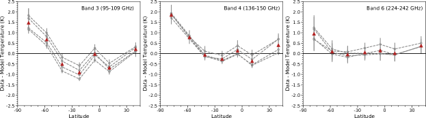
Figure 11: As Fig. 10, but allowing only CH₄ to vary with latitude. We find CH₄ profiles that match the Band 6 data and compare these with the Band 3 and Band 4 data.

4.4.3 Varying ortho/para H₂

In these fits, we consider the fraction of equilibrium H₂ to normal H₂ needed to match the Band 6 brightness temperatures. Since normal H₂ decreases the brightness temperature, adding normal H₂ to latitudes with positive temperature residuals (like the south pole) is implausible. Figure 12 plots the temperature residuals in each band. We find that a hydrogen mixture of 90$\%$ equilibrium hydrogen and 10$\%$ normal hydrogen can explain the Band 6 data between 32^∘S$-12^{\circ}$S, with equilibrium H₂ used everywhere else. However, the other ALMA spectral bands fail to fit the data from 32^∘S$-12^{\circ}$S. This result is expected based on the spectral analysis in figure 8, showing the minimal effect normal hydrogen has in Band 3. For the best fit model, we therefore do not consider normal hydrogen. We emphasize however that our results do not preclude a small fraction of normal H₂, on the order of $\leq 10\%$, existing at the pressures probed by ALMA. This is consistent with findings from Voyager IRIS measurements (Conrath et al., 1998; Fletcher et al., 2014. These studies find that the para H₂ fraction deviates from its expected equilibrium values on the order of $2-5\%$ between $0.01-1$ bar.

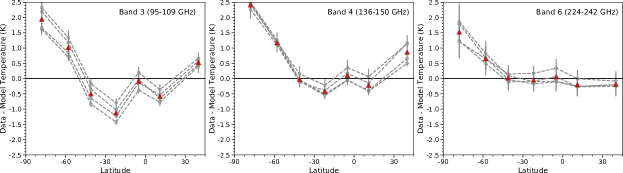
Figure 12: As Fig. 10, but allowing only the fraction of equilibrium H₂ to vary with latitude. We find H₂ profiles that match the Band 6 data and compare these with the Band 3 and Band 4 data.

4.4.4 Best Fit Model

The first row in Table 4 describes the H₂S and CH₄ profiles that provide a best fit to the data in all ALMA bands in each latitudinal bin. Figure 13 plots colormaps of the best fit profiles versus latitude. Figure 14 plots the temperature residuals in each band, showing that an excellent fit is obtained at all latitudes. In general, we find that bright regions in the residual maps require depleting H₂S and sometimes CH₄ (down to $\sim 0.6-1.1\%$), while dark regions require supersaturing H₂S and enhancing the deep CH₄ abundance ($\sim 2.2-2.9\%$) to fit the data in every band.

4.4.5 Comparison to Karkoschka & Tomasko, 2011

Karkoschka & Tomasko (2011) determined methane mixing ratios from the HST/STIS spectrograph data between $300-1000$ nm across Neptune’s disk. Their results are consistent with a constant deep methane mixing ratio of $4\pm 1\%$ at $P>3.3$ bar. However, between $1.2-3.3$ bar, they argued that the methane mixing ratio was depressed by a factor of $\sim 3$ at Neptune’s mid-latitudes compared to the equator. Not only is their deep methane mixing ratio significantly higher than our best fit models (ranging between $0.6-2.9\%$), but their observed trend in the methane abundance across Neptune’s disk differs from ours. We find high methane mixing ratios relative to the nominal model between $32^{\circ}$S$-12^{\circ}$S and $2^{\circ}$N$-20^{\circ}$N, and low abundances from $90^{\circ}$S$-66^{\circ}$S and $12^{\circ}$S$-2^{\circ}$N. The ALMA Band 6 contribution functions peak at $P<4$ bar, so we expect some signature of the opacity from $1.2-3.3$ bar to appear in our results.

In order to test the models presented in Karkoschka & Tomasko (2011) to our data, we compare how the H₂S abundance must change to fit the data in every band. Between $32^{\circ}$S$-20^{\circ}$N, we use the Karkoschka & Tomasko (2011) methane profile at $6^{\circ}$S; elsewhere, we use their $45^{\circ}$S model (see their Figs. 10 and 14). The one exception is at the south pole cap, $90^{\circ}$S$-66^{\circ}$S, where we use our best fitting profile since the deep H₂S abundance is fairly well constrained in VLA data.

Since the Band 6 data have the most overlap with the analysis in Karkoschka & Tomasko (2011) in terms of altitude, we find the H₂S profiles at each latitude that fit Band 6 well, assuming their adopted CH₄ profiles and equilibrium H₂. Our results are plotted in Figure 15 and a full description of the model and corresponding statistics is listed in Tables 4 and 5. We can find H₂S profiles which result in generally good agreement between the model and data only from $90^{\circ}$S$-50^{\circ}$S and northward of $20^{\circ}$N. In this case, the disk-averaged H₂S abundance is $\sim 10\times$S. Luszcz-Cook & de Pater (2013a) computed the disk-averaged brightness temperature assuming a 10$\times$S model, showing that the brightness temperature is too high in this case compared to most of the radio data (see also Fig. 3). Therefore, our data are not consistent with the Karkoschka & Tomasko (2011) methane profiles. We address this in the following section.

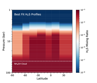
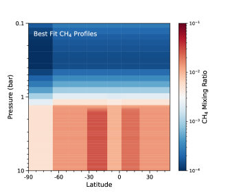
Figure 13: Left: Best fit H₂S vertical profiles versus latitude. Right: Best fit CH₄ vertical profiles versus latitude. These profiles are the same as those listed in the first row of Table 4. The colors represent volume mixing ratios, with high abundances in red and low abundances in blue. Note the different pressure and mixing ratio scales between the two figures.

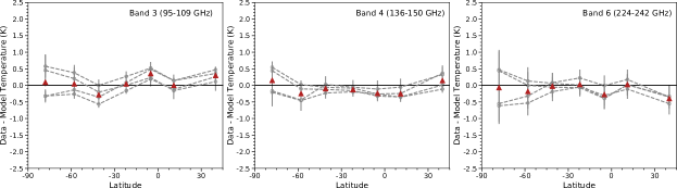
Figure 14: As Figure 10, but using the best fit H₂S and CH₄ profiles.

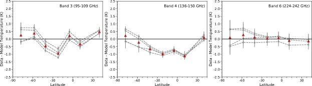
Figure 15: As Figure 5, but using the CH₄ profiles from Karkoschka & Tomasko, 2011 and finding the H₂S profiles that best match Band 6.

Table 4: Model names and their constituent profiles in each latitude bin that give a best fit to the data.

Model Name	90∘S$-66^{\circ}$S	66∘S$-55^{\circ}$S	55∘S$-32^{\circ}$S	32∘S$-12^{\circ}$S	12∘S$-2^{\circ}$N	2∘N$-20^{\circ}$N	20∘N$-50^{\circ}$N
Best Fit	H2S 1.5$\times$S CH4 0.55$\%$ H2 equil.	H2S 10$\times$S CH4 1.44$\%$ H2 equil.	H2S 30$\times$S CH4 1.44$\%$ H2 equil.	H2S supersat-v1 CH4 2.88$\%$ H2 equil.	H2S 20$\times$S CH4 1.08$\%$ H2 equil.	H2S supersat-v1 CH4 2.16$\%$ H2 equil.	H2S 10$\times$S CH4 1.44$\%$ H2 equil.
Vary H2S Only	H2S 1.5$\times$S CH4 0.55$\%$ H2 equil.	H2S 10$\times$S CH4 1.44$\%$ H2 equil.	H2S 30$\times$S CH4 1.44$\%$ H2 equil.	H2S supersat-v2 CH4 1.44$\%$ H2 equil.	H2S 3$\times$S CH4 1.44$\%$ H2 equil.	H2S supersat-v2 CH4 1.44$\%$ H2 equil.	H2S 3$\times$S CH4 1.44$\%$ H2 equil.
Vary CH4 Only	H2S 30$\times$S CH4 0.55$\%$ H2 equil.	H2S 30$\times$S CH4 0.55$\%$ H2 equil.	H2S 30$\times$S CH4 1.44$\%$ H2 equil.	H2S 30$\times$S CH4 2.88$\%$ H2 equil.	H2S 30$\times$S CH4 1.44$\%$ H2 equil.	H2S 30$\times$S CH4 1.44$\%$ H2 equil.	H2S 30$\times$S CH4 0.55$\%$ H2 equil.
Vary H2 Only	H2S 30$\times$S CH4 0.55$\%$ H2 equil.	H2S 30$\times$S CH4 1.44$\%$ H2 equil.	H2S 30$\times$S CH4 1.44$\%$ H2 equil.	H2S 30$\times$S CH4 1.44$\%$ H2 90$\%$ equil.	H2S 30$\times$S CH4 1.44$\%$ H2 equil.	H2S 30$\times$S CH4 1.44$\%$ H2 equil.	H2S 30$\times$S CH4 1.44$\%$ H2 equil.
KT2011a CH4	H2S 1.5$\times$S CH4 0.55$\%$ H2 equil.	H2S 5$\times$S CH4 45S H2 equil.	H2S 15$\times$S CH4 45S H2 equil.	H2S $15\times$S CH4 6S H2 equil.	H2S 10$\times$S CH4 6S H2 equil.	H2S 10$\times$S CH4 6S H2 equil.	H2S 5$\times$S CH4 45S H2 equil.

^a KT2011 refers to Karkoschka & Tomasko, 2011. CH₄ 45S and 6S refer to their adopted methane profiles at those latitudes in their Figs. 10 and 14

Model Name	90∘S-66∘S	66∘S-55∘S	55∘S-32∘S	32∘S-12∘S	12∘S-2∘N	2∘N-20∘N	20∘N-50∘N
Best Fit	3.4	2.9	6.8	2.0	8.1	4.1	6.2
Vary H2S Only	3.4	2.6	3.2	14.8	46.4	13.0	7.5
Vary CH4 Only	55.8	20.7	16.5	56.7	2.3	25.5	7.3
Vary H2 Only	95.8	48.0	16.1	85.6	2.8	17.2	29.0
KT2011 CH4 Only	3.9	4.3	28.9	100.4	20.9	50.3	8.8

Table 5: Reduced $\chi^{2}$ values versus latitude bin per model. Bold values are significant at the $p\leq 0.05$ level, meaning the model at those latitudes is inconsistent with the observations.

5 Discussion

5.1 Neptune’s South Polar Cap

Our ALMA millimeter observations provide a glimpse of Neptune’s atmosphere situated between the deep troposphere in centimeter maps ($P\geq 10$ bar) and the upper troposphere and stratosphere in the visible and infrared. The constraints on the trace gases are useful to infer the dynamics of Neptune’s atmosphere. Of particular interest is Neptune’s south pole, whose high temperatures were first published by Hammel et al. (2007) with images taken with the Gemini north telescope at 7.7$\mu$m and 11.7$\mu$m. They suggested these bright regions are due to enhancements in ethane and methane. Orton et al. (2007) imaged atmospheric line-free thermal emission of Neptune with the Very Large Telescope in 2006, finding temperature excesses of $10-11$K and $3-5$K near, but not at, Neptune’s south pole at 17.6$\mu$m and 18.7$\mu$m respectively. These authors suggested that seasonal warming around Neptune’s south pole could explain why the stratospheric abundance of methane is larger than expected; cold temperatures should result in methane condensing and becoming trapped below the tropopause. However, warm polar temperatures may allow methane gas to escape upward into the stratosphere and diffuse across the globe.

Warm brightness temperature measurements at high-latitudes are persistent throughout radio maps. de Pater et al. (2014) found temperature enhancements from 8$-$30K in VLA 1.3$-$6.2 cm maps, where sensitivities peak between $5-50$ bar. EVLA 1-cm maps show enhancements of similar magnitudes southward of 70^∘S (Butler et al., 2012). Luszcz-Cook et al. (2013b) see southern high-latitude enhancements of $2-3$K compared to the northern mid-latitudes in 1.2 mm CARMA maps. Our ALMA maps show average enhancements of $2-3$K in Bands 3 and 4, with sensitivities peaking at $P>1$ bar, and $1-2$K in Band 6, whose sensitivities peak at 1 bar. Iino & Yamada (2018) analyzed ALMA flux calibration data of Neptune at 646 GHz (0.46 mm), peaking at 0.6 bar, and ruled out a detection of the south polar hot spot greater than 2.1K compared to the background. Combined, these data suggest that the magnitude of the south polar brightness enhancements decreases with increasing altitude. This trend is likely due to the temperature-pressure profile, which is mostly isothermal between $0.1-1$ bar. This picture also appears dynamically distinct from that described in Orton et al. (2007), who predicted upwelling air to explain methane and ethane enrichment in the stratosphere. In the radio, brightness enhancements are consistent with low-opacity (dry) air so deeper warmer layers are probed. The air is likely subsiding, after having been dried out at other latitudes. The subsiding air causes adiabatic warming, which is sensed in the mid-IR (e.g., Fig. 16 in de Pater et al. (2014)). Persistent cloud activity surrounding Neptune’s south pole may be indicative of vigorous convection and evidence of a south polar vortex (Luszcz-Cook et al., 2010), analogous to the polar activity seen on Saturn (Fletcher et al., 2008; Dyudina et al., 2008). Such a system could explain the observed temperature, ethane and methane enhancements in the mid-IR, polar cloud features seen with Voyager and Keck, and high brightness temperatures in the radio.

Recent findings by Irwin et al. (2019) find a tentative detection of an H₂S spectral signature between $1.57-1.58\mu$m on Neptune with Gemini-North/NIRS. They find that the signature is stronger at southern latitudes than at the equator, with H₂S abundances around 3 ppm and 1 ppm respectively at the top of Neptune’s H₂S cloud deck: $2.5-3.5$ bar. This broadly agrees with our suite of proposed H₂S profiles (Fig. 9), where H₂S is depleted to an abundance of 1 ppm between $\sim 2.5-4$ bar. The exception is our model for the south polar cap, which has less H₂S at the relevant altitudes than predicted by Irwin et al. (2019). In order to match their results, we would have to lower the altitude where H₂S follows the saturated vapor pressure curve (to $P>4.5$ bar) so that the abundance from $2.5-3.5$ bar could be increased to 1 ppm. Moreover, their retrieved H₂S abundances are most consistent with models which deplete the deep abundance of CH₄ at the southern high-latitudes relative to the equator. This agrees with our results and Karkoschka & Tomasko (2011).

5.2 Neptune’s Mid-Latitudes and Equator

Moving northward, our ALMA maps show that latitudes spanning $32^{\circ}-12^{\circ}$S and $2^{\circ}-20^{\circ}$N are colder than the background by $\sim 0.5-1.5$K in all three bands. This difference can only be explained at all wavelengths with models which both increase the deep CH₄ abundance to $\sim 2.2-2.9\%$ and supersaturate the H₂S profile. This is consistent with upwelling, adiabatically cooling plumes, and the observed distribution of prevalent bright cloud activity in this latitude range seen in the visible and near-IR. Karkoschka & Tomasko (2011) find that methane is well-mixed in the deep-atmosphere, with an abundance of $4\pm 1\%$. In addition, they find that methane is depleted by a factor of 3 at the southern mid-latitudes compared to the equatorial region between 1.2 and 3.3 bar. This pressure range contributes the most to the opacity in Band 6, wavelengths where we also see the lowest temperature contrasts. If we assume their horizontal methane profiles, our models are too cold to match the ALMA data, due to their high methane abundance. A corresponding global decrease in the H₂S abundance to $\sim 10\times$S must be made in order to decrease the total opacity and increase the brightness temperature so that the Band 6 data and model agree. However, decreasing the global H₂S abundance has the side effect of dramatically increasing the brightness temperatures in Bands 3 and 4, particularly near the equator. In Band 4, these profiles fit the equatorial regions poorly, yet agree at these latitudes in Band 3. For Band 4 to match here, the H₂S abundance would have to be increased to account for a 1 K difference. However, the Band 3 model temperatures would be decreased by at least this same amount, putting it outside a two-sigma fit to the data. Moreover, model disk-averaged brightness temperatures assuming a $10\times$ S H₂S abundances are too warm compared to the ALMA and 2003 VLA data (Fig. 3).

Our results are more consistent with Baines et al. (1995), who predict disk-averaged deep-atmosphere methane molar fractions of $2.2^{+0.5}_{-0.6}\%$. Karkoschka & Tomasko (2011) remark that the two studies use different haze and cloud profiles and relative humidities. Correcting for these factors lowers their deep-atmosphere methane mixing ratio to within the error bars cited in Baines et al. (1995). In addition, Karkoschka & Tomasko (2011) note that a significant contribution to their error bars is due to systematic variations in their center-to-limb profiles in the methane bands. Their model is too bright at disk center and too cold at the limb. Lowering the methane mixing ratio and using different values for the (poorly known) methane and hydrogen absorption coefficients would improve their fit. Alternatively, a high deep methane mixing ratio may be possible if methane is subsaturated, which we did not consider in our models. Subsaturated models will produce warmer brightness temperatures while increasing the deep methane mixing ratio will produce colder temperatures. As a result, these effects will partially cancel and combined may produce a more reasonable fit. There may also be uncertainties in the millimeter spectral line parameters that are not accounted for here. Laboratory measurements of H₂S absorption in the millimeter are extremely limited and not at Neptune’s tropospheric conditions (Joiner et al., 1992). Updated measurements of the trace gas absorption lines under cold, ice giant conditions would improve, and perhaps reconcile, models of these multi-wavelength observations.

While we disagree with the deep methane mixing ratio computed by Karkoschka & Tomasko (2011), we find general agreement with their observed latitude trends. Both our study and theirs find enhancements in trace gases from $32^{\circ}-12^{\circ}$S and $2^{\circ}-20^{\circ}$N, depletion from $90^{\circ}-50^{\circ}$S and north of 20^∘N, and intermediate values from $50^{\circ}-32^{\circ}$S. Our sole inconsistency is from $12^{\circ}$S$-2^{\circ}$N, where we also depleted trace gases. However, at these latitudes, Karkoschka & Tomasko (2011) lowered the tropospheric haze optical depth compared to the surrounding latitudes. If their haze optical depth was increased here, we would expect them to need to decrease the methane abundance from $12^{\circ}$S$-2^{\circ}$N to fit their data. Luszcz-Cook et al. (2016) also investigated methane profiles in cloud free regions of Neptune with the OSIRIS integral field spectrograph in the H and K broad bands. These data probe altitudes higher than ALMA and HST/STIS and so are insensitive to the deep troposphere methane abundance. These authors saw tentative evidence of meridional variations in the methane profile, qualitatively consistent with Karkoschka & Tomasko (2011), but remarked that their parameterizations could not fully characterize the true shape of the methane profile since they were only sensitive to $P<2.5$ bar.

In the equatorial region, our ALMA residual maps show clear latitudinal structure undetected in prior radio studies of Neptune. North of the equator, we detect low brightness temperatures that are consistent with supersaturating H₂S and a slight increase in the deep CH₄ abundance. In the visible and near-IR, Neptune’s equatorial region is quiescent, lacking bright cloud activity compared to the dramatic stormy mid-latitudes. However, there is evidence of more cloudy activity just north of the equator than south of it, agreeing with our finding of CH₄ enrichment from $2^{\circ}-20^{\circ}$N and depletion from $12^{\circ}$S$-2^{\circ}$N. Figure 16 shows a histogram counting the number of bright cloud features versus latitude from Voyager, the Hubble Space Telescope, and H-band Keck maps which were tracked in five papers: Limaye & Sromovsky (1991); Sromovsky et al. (2001); Martin et al. (2012); Fitzpatrick et al. (2014); Tollefson et al. (2018). By eye, there appears to be a clear correlation between our ALMA defined latitude bands and latitudes where the number of features transitions from low-to-high or vice-versa, particularly in the Voyager data. This suggests that the banded structure seen by ALMA from $1-10$ bar exists up to the visible cloud deck. Specifically, at the central latitudes within the 12^∘S$-$2^∘S band, there is a persistent scarcity of activity observed over a 30 year period. In contrast, features are seen regularly between 2^∘S$-$20^∘N, suggesting a larger source of condensible methane. This agrees with our best fit model which depletes CH₄ to $\sim 1.1\%$ in the cloud-free latitudes and enriches it to $\sim 2.2\%$ in the cloud-prevalent latitudes. The enhancement of methane in this region is consistent with a moist convective origin of a recently discovered large bright storm centered at 2^∘N (Molter et al., 2019). Moreover, this model may explain inconsistencies between the thermal wind equation and observed vertical wind shear measurements. Fitzpatrick et al. (2014) and Tollefson et al. (2018) detected vertical wind shear at Neptune’s equator by tracking bright cloud features in the H- and K’-bands with Keck, with the K’-band probing higher altitudes with features that have, on average, stronger retrograde velocities than features seen in the H-band. Tollefson et al. (2018) showed that the equator must be methane-rich and warm compared to mid-latitudes if the thermal wind equation holds.

Figure 16: Histogram counting the number of tracked bright cloud features versus latitude. Dashed lines delineate the latitude bands used in the modeling of the ALMA data and correspond to variations in the residual brightness temperature. Counts are in one-degree latitude bins and latitudes have been converted to planetographic coordinates. Since the Voyager data would otherwise dominate the count and perceived trend, these data are split apart, showing the Voyager counts on the left and post-Voyager counts on the right. These data come from five papers, labeled as follows: Li91 - Limaye & Sromovsky, 1991; Ma12 - Martin et al., 2012; To18 - Tollefson et al., 2018; Fi14 - Fitzpatrick et al., 2014; Sr01 - Sromovsky et al., 2001.

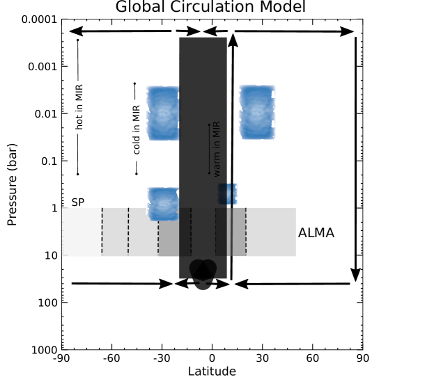
Figure 17: Schematic of Neptune’s global circulation inferred from ALMA observations, adapted from Fig. 21 in de Pater et al. (2014). Black arrows outline the circulation pattern, which extends from the stratosphere down to 40 bar. The biggest change from the sketch in de Pater et al. (2014) is our circulation cells are narrowed near the equator and we prefer a subsiding region which is just south of the equator (aligning with the $12^{\circ}$S$-2^{\circ}$N range seen in our residual map), instead of hemispheric symmetric cells. The gray rectangle between $1-10$ bar shows the sensitivity of the ALMA spectral bands (see Fig. 1). Dark-gray (off-white) rectangles are the latitude ranges where the residual brightness temperature is colder (warmer) than the background (see Fig. 4). At these latitudes, both H₂S and CH₄ are enriched (depleted) (see Table 5). The light-gray rectangles are latitude ranges where the residual brightness temperature is similar to the background. Here, H₂S and CH₄ equal their nominal value, or only H₂S is depleted. The locations of Visible/NIR clouds are illustrated with blue vertical patches. Most clouds are seen at the mid-latitudes (peak cloud counts are centered near $25^{\circ}$S and $30^{\circ}$N, see Fig. 15) and are seen high in the atmosphere (e.g., those tracked in de Pater et al. (2014)). However, clouds just north of the equator are also seen and are deeper in the atmosphere (de Pater et al. (2014), Tollefson et al. (2018), and Fig. 15). Neptune’s south polar feature (SPF) and south polar (SP) cloud are also placed. Marked cloud layers (CH₄-ice, H₂S-ice, NH₄SH, H₂O-ice, Solution Cloud) on the right are assumed to be independent of latitude (see Fig. 1). Also indicated are where high and low temperatures are measured in the MIR (Fletcher et al. 2014). Poleward of $\sim 50^{\circ}$N, seeing is cut off in all observations as Neptune’s north pole is tilted away from the observer (rectangular diagonal hatches). Downwelling motions are assumed at Neptune’s north pole in order to complete the circulation diagram.

The thermal profile inferred from MIR observations, the horizontal distribution of clouds, and observed regions of enriched/depleted air all relate to vertical circulation motions. Based on multi-wavelength observations, de Pater et al. (2014) suggest a vertically extended, hemispheric symmetric double-cell pattern with upwelling at the mid-latitudes and downwelling at the equator and poles from the stratosphere down to the deep troposphere ($\sim$40 bar). The ALMA, HST/STIS, and OSIRIS results suggest more detailed circulation, particularly near the equator. Our analysis is consistent with the prediction of vertically extended cells, going from the stratosphere down to $\sim 40$ bar, since there is a clear alignment between the ALMA detected latitudinal bands and the observed distribution of cloud features. However, we argue that the equatorial region is more intricate than what was outlined by de Pater et al. (2014), with upwelling from 2^∘N$-$20^∘N and downwelling from 12^∘S-2^∘N. A narrower circulation cell than predicted by de Pater et al. (2014) centered just south of the equator would partially explain the differing predictions between these studies. Figure 17 gives a sketch of our proposed global circulation pattern.

6 Conclusion

Spatially resolved millimeter maps of Neptune are presented in three ALMA bands, spanning $95-242$ GHz. These maps have unprecedented sensitivities in the millimeter, ranging between $0.1-0.6$K, and resolutions down to $0.3"$, roughly one-eighth of Neptune’s diameter. The observed emission is mainly modulated by the opacity due to H₂S absorption, CIA of H₂ with H₂, He, and CH₄, and ortho/para H₂. We used the radiative transfer code Radio-BEAR to vary the abundance profiles of these gases in order to model the brightness temperature across Neptune’s disk. Our main conclusions are as follows:

1. The disk-averaged brightness temperature of Neptune in the millimeter and centimeter matches a model where: the temperature-pressure profile follows a dry adiabat; H₂S, CH₄, and H₂O are enriched by 30$\times$ their protosolar values, while NH₃ is held at $1\times$ its protosolar value; intermediate H₂ is assumed. This is referred to as the ‘nominal’ model.

2. Subtracting the nominal beam-convolved model from the data shows clear brightness temperature variations across Neptune’s disk. We identify latitudes in between significant transitions in the brightness temperature: 90${}^{\circ}-66^{\circ}$S, 66${}^{\circ}-55^{\circ}$S, 55${}^{\circ}-32^{\circ}$S, 32${}^{\circ}-12^{\circ}$S, 12^∘S$-$2^∘N, 2${}^{\circ}-20^{\circ}$N, and northward of 20^∘N. These bands are at least the size of the ALMA synthesized beam and are apparent in all maps. Relative to the nominal model, brightness enhancements of $1-3$K are seen at $90^{\circ}$S$-$$66^{\circ}$S and $66^{\circ}$S$-$$55^{\circ}$S. Negative temperature residuals between $0.5-1.5$K are seen from 32${}^{\circ}-12^{\circ}$S and 2${}^{\circ}-20^{\circ}$N. These bands align with regions transitioning from high or low counts in the number of cloud features versus latitude, suggesting that the banded structure we see in the ALMA data exists up at the visible cloud deck. As a result, these identified latitudinal bands may be indicative of a zonal wind profile that is more complex than hitherto considered.

3. At the south polar cap, our best fit model depletes the deep atmospheric abundance of both H₂S to 1.5$\times$ the protosolar value and CH₄ to 0.55$\%$ (11.5$\times$S). This is consistent with models fitting VLA and CARMA data (de Pater et al., 2014; Luszcz-Cook et al., 2013b). Between 55${}^{\circ}-32^{\circ}$S and northward of 20^∘N, our best fit models deplete H₂S to $10\times$S while keeping CH₄ at the nominal value of 1.44$\%$ (30$\times$S). From 32${}^{\circ}-12^{\circ}$S and 2^∘N$-$20^∘N, H₂S is supersaturated and the deep abundance of CH₄ is enriched to $2.2-2.9\%$ ($45-60\times$S). From 12^∘S$-2^{\circ}$N, we deplete H₂S to 10$\times$ protosolar and CH₄ to 1.1$\%$ ($22.5\times$S). Warm brightness temperatures relative to the nominal model are consistent with dry, subsiding air. Conversely, cold brightness temperatures are consistent with moist, rising air. Our results are, therefore, consistent with an intricate global circulation system that extends from the cloud deck to deep in the atmosphere.

These ALMA maps are evidence of a more complex zone and belt structure that may be yet unresolved in the zonal wind field. An ice-giant probe and high-resolution spacecraft imaging characterizing the zonal wind structure in detail would help settle any inconsistencies between Neptune’s velocity, thermal, and compositional profiles.

7 Acknowledgements

The authors wish to thank Arielle Moullet for helping with the data reduction and imaging process. This work has been supported in part by the National Science Foundation, NSF Grant AST-1615004 to UC Berkeley and by NASA Headquarters: under the NASA Earth and Space Science Fellowship program Grant NNX16AP12H to UC Berkeley.

This paper makes use of the following ALMA data: ADS/JAO.2016.1.00859.S. ALMA is a partnership of ESO (representing its member states), NSF (USA) and NINS (Japan), together with NRC (Canada), NSC and ASIAA (Taiwan), and KASI (Republic of Korea), in cooperation with the Republic of Chile. The Joint ALMA Observatory is operated by ESO, AUI/NRAO and NAOJ. The National Radio Astronomy Observatory is a facility of the National Science Foundation operated under cooperative agreement by Associated Universities, Inc.

References

- Asplund et al. (2009) Asplund, M., Grevesse, N., Sauval, A. J., Scott, P., 2009, Annual Review of Astronomy and Astrophysics, 47, 481
- Baines et al. (1995) Baines, K. H., Mickelson, M. E., Larson, L. E., Ferguson, D. W., 1995, Icarus, 114, 328
- Brogan et al. (2018) Brogan, C. L., Hunter, T. R., Fomalont, E. B., 2014, in the Proceedings of the 2014 Synthesis Imaging Workshop held in Socorro, NM on May 13-20, 2014
- Butler et al. (2012) Butler, B. J., Hofstadter, M., Gurwell, M., Orton, G., Norwood, J., 2012. in AAS/Division for Planetary Sciences Meeting Abstracts, Vol. 44, 504.06
- Conrath et al. (1998) Conrath, B., Gierasch, P., Ustinov, E. A., 1998, Icarus, 135, 501
- Conrath et al. (1991) Conrath, B. J., Flasar, F. M., Gierasch, P. J., 1991, JGRA, 96, 18931
- de Pater et al. (2014) de Pater, I., Fletcher, L. N., Luszcz-Cook, S., et al. 2014, Icarus, 237, 211
- de Pater & Massie (1985) de Pater, I. & Massie, S. T., 1985, Icarus 62, 143
- de Pater & Mitchell (1993) de Pater, I., Mitchell, D. L., 1993, JGRE, 98, 5471
- de Pater & Richmond (1989) de Pater, I. & Richmond, M., 1989, Icarus, 80, 1
- de Pater et al. (1991) de Pater, I., Romani, P. N., Atreya, S. K., 1991, Icarus, 91, 220
- de Pater et al. (2019) de Pater, I., Sault, R., Wong, M. H., et al. 2019, Icarus, 322, 168
- Dyudina et al. (2008) Dyudina, U. A., Ingersoll, A. P., Ewald, S. P., et al. 2008. Science, 319, 1801
- Fitzpatrick et al. (2014) Fitzpatrick, P. J., de Pater, I., Luszcz-Cook, S., Wong, M. H., Hammel, H. B., 2014, Ap&SS, 350, 65
- Fletcher et al. (2010) Fletcher, L. N., Achterberg, R. K., Greathouse, T. K., et al. 2010, Icarus, 208, 337
- Fletcher et al. (2014) Fletcher, L. N., de Pater, I., Orton, G. S., et al. 2014, Icarus, 231, 146
- Fletcher et al. (2008) Fletcher, L. N., Irwin, P. G. J., Orton, G. S., et al. 2008. Science, 319, 79
- Hammel et al. (2007) Hammel, H. B., Sitko, M. L., Lynch, D. K., et al. 2007, AJ, 134
- Iino & Yamada (2018) Iino, T. & Yamada, T., 2018, AJ, 155, 92.
- Irwin et al. (2019) Irwin, P. G., Toledo, D., Garland, R., et al. 2019. Icarus, 321, 550
- Joiner et al. (1992) Joiner, J., Steffes, P. G., Noll, K. S., 1992. ITMTT, 40, 1101