AutoAssist: A Framework to Accelerate Training of Deep Neural Networks

Abstract

Deep neural networks have yielded superior performance in many applications; however, the gradient computation in a deep model with millions of instances leads to a lengthy training process even with modern GPU/TPU hardware acceleration. In this paper, we propose AutoAssist, a simple framework to accelerate training of a deep neural network. Typically, as the training procedure evolves, the amount of improvement in the current model by a stochastic gradient update on each instance varies dynamically . In AutoAssist, we utilize this fact and design a simple instance shrinking operation, which is used to filter out instances with relatively low marginal improvement to the current model; thus the computationally intensive gradient computations are performed on informative instances as much as possible. We prove that the proposed technique outperforms vanilla SGD with existing importance sampling approaches for linear SVM problems, and establish an $O(1/k)$ convergence for strongly convex problems. In order to apply the proposed techniques to accelerate training of deep models, we propose to jointly train a very lightweight Assistant network in addition to the original deep network referred to as Boss. The Assistant network is designed to gauge the importance of a given instance with respect to the current Boss such that a shrinking operation can be applied in the batch generator. With careful design, we train the Boss and Assistant in a nonblocking and asynchronous fashion such that overhead is minimal. We demonstrate that AutoAssist reduces the number of epochs by $40\%$ for training a ResNet to reach the same test accuracy on an image classification data set, and saves $30\%$ training time needed for a transformer model to yield the same BLEU scores on a translation dataset.

1 Introduction

Deep neural networks trained on a large number of instances have been successfully applied to many real world applications, such as [8, 11] and [21]. Due to the increasing number of training instances and the increasing complexity of deep models, variants of (mini-batch) stochastic gradient descent (SGD) are still the most widely used optimization methods because of their simplicity and flexibility. In a typical SGD implementation, a batch of instances is generated either by using a random permuted order or a uniform sampler. Due to the complexity of deep models, the gradient calculation is usually extremely computationally intensive and requires powerful hardware (such as a GPU or TPU) to perform the entire training in reasonable time. At any given time of the learning, each instance has its own utility in terms of improving the current model. As a result, performing SGD updates on a batch of instances which are sampled/generated uniformly is suboptimal in terms of maximization of return-on-investment (ROI) of GPU/TPU cycles. In this paper, we propose AutoAssist, a simple framework to accelerate training deep models with an Assistant that generates instances in a sequence which attempts to maximize the ROI.

There have been attempts to improve the training speed of deep learning. In [3], curriculum learning (CL), where “easier” instances are presented earlier than “harder” instances, was shown to be beneficial to the overall convergence; however, prior knowledge of the training set is required to rank the instances by its simplicity or difficulty. Self-paced learning (SPL) [20] is another attempt that infers the “difficulty” of instances based on the corresponding loss value during training and decreases the sample probability of these difficult instances, which, however, ends up overly emphasizing the easier samples. However, the marginal gain of information provided by these easier instances decreases as the model gets better, which leads to slow convergence of SPL. [13] combined the above two ideas and proposed Self Paced Curriculum learning (SPCL), which is formulated as an optimization problem which utilizes both prior knowledge and the loss values as the learning progresses. However SPCL relies on a manually chosen scheme function which has $O(N)$ parameters to be learned, where $N$ is number of instances in the dataset, which introduces a considerable overhead into the training process in terms of both time and space complexity.

In this paper, we propose AutoAssist, a simple framework to accelerate training deep models with an Assistant that generates instances in a sequence which attempts to maximize the ROI. In particular, the main model, referred to as the Boss, is trained with instances generated by a light-weight Assistant, which yields instances in a sequence that tries to maximize the ROI for the current Boss. In particular, the Assistant is designed in a way to adapt to the changes in Boss dynamically and asynchronously. Our contributions in this paper are as follows.

• We propose an AutoAssist learning framework with an Assistant which can shrink less informative instances and generate smart batches in an ROI aware sequence to the Boss to perform SGD updates. We also propose a computational scheme so that learning of the Boss and the Assistant are done asynchronously, which minimizes the overhead introduced by the Assistant.

• We prove that even with biased stochastic gradient, the instance shrinking method based on gradient magnitude can still guarantee the $O(\frac{1}{k})$ convergence achieved by plain SGD under the strongly convex setting.

• We empirically show that the proposed AutoAssist framework leads to improved convergence as well as test loss on various deep learning applications, including image classification and neural machine translation.

2 Related Work

Considerable research has been conducted to optimize the way data is presented to the optimizer for deep learning. For example, curriculum learning (CL) [3], which presents easier instances to the model before hard ones, was shown to be beneficial to the overall convergence; however, prior knowledge of the training set is required to decide the curriculum. Self-paced learning (SPL) [20] infers the difficulty of instances with the corresponding loss value and then decreases the sample probability of difficult instances. Self-paced Convolutional Networks (SPCN) [23] combines the SPL algorithm with the training of Convolutional Neural Networks to get rid of noisy data. However, the SPL type methods usually result in over emphasis of the easier instances and thus harm performance. Similar ideas have been developed when optimizing for other machine learning models. In classical SVM models, methods have been proposed to ignore trivial instances by dimension shrinking in dual coordinate descent. This accelerates the convergence speed by saving many useless parameter updates.

Importance sampling is another type of method that has been proposed to accelerate SGD convergence. In importance sampling methods, instances are sampled by its importance weights. [31] proposed Iprox-SGD that uses importance sampling to achieve variance reduction. The optimal importance weight distribution to reduce the variance of the stochastic gradient is proved to be the gradient norm of the sample [24, 31, 1]. Despite the variance reduction effect, importance sampling methods tend to introduce large computational overhead. Before each stochastic step, the importance weights need to be updated for all instances which makes importance sampling methods infeasible for large datasets. [15] proposed an importance sampling scheme for deep learning models; however, in order to reduce computation cost for evaluating importance scores, the proposed algorithm applied a sub-sampling technique, thus leading to reliance on outdated importance scores for training.

There are also several recent methods that propose to train an attached network with the original one. ScreenerNet [17] trains an attached neural network to learn a scalar weight for each training instance, while MentorNet [14] learns a data-driven curriculum that prevents the main network from over-fitting. Since the additional model is another deep neural network, these types of methods introduce substantial computational and memory overhead to the original training process.

Unlike previous methods, our proposed AutoAssist framework (1) does not need prior knowledge of the task, (2) is able to utilize the response of the latest deep model to pick informative training instances, and (3) can greatly reduce overhead through CPU/GPU asynchronous training.

3 Dual coordinate shrinking vs primal instance shrinking

In this section, we motivate our methodology by introducing the shrinking algorithm in dual coordinate descent of support vector machines (SVMs) and showing that it is the same as ignoring certain instances in primal stochastic gradient descent.

3.1 Shrinking in dual coordinate descent

Consider the SVM for data classification. Given a set of instance-label data pairs $\{{\bm{x}}_{i},y_{i}\}_{i\in[N]}$ where ${\bm{x}}_{i}\in\mathcal{R}^{n}$ and $y_{i}\in\{+1,-1\}$, SVM tries to solve the following minimization problem:

$$\min_{{\bm{w}}}\frac{1}{2}{\bm{w}}^{\top}{\bm{w}}+C\sum_{i=1}^{N}l({\bm{w}},{\bm{x}}_{i},y_{i}),$$ (1)

where $C>0$ and loss function $l$ defined as:

$$l({\bm{w}},{\bm{x}}_{i},y_{i})=\max(1-y_{i}{\bm{w}}^{\top}{\bm{x}}_{i},0).$$ (2)

The form (1) is often referred to as the primal form of SVM. By Representer Theorem, the primal parameter can be written as:

$${\bm{w}}=\sum_{j=1}^{N}\alpha_{j}y_{j}{\bm{x}}_{j}$$ (3)

for some $\bm{\alpha}\in\mathcal{R}^{N}$, thus we can solve the following dual form instead:

$$\min_{\bm{\alpha}} \>f(\bm{\alpha})=\frac{1}{2}\bm{\alpha}^{\top}\bm{{Q}}\bm{\alpha}-{\bm{e}}^{\top}\bm{\alpha}$$ (4)

$$s.t. \>0\leq\alpha_{i}\leq C,\forall i,$$

where $Q_{ij}=y_{i}y_{j}{\bm{x}}_{i}^{\top}{\bm{x}}_{j}$. The above dual form is usually solved by cyclic coordinate descent; during training step $k$, the update rule for coordinate $i$ is given by:

$$\alpha_{i}^{k+1}=\min\mathopen{}\mathclose{{}\left(\max\mathopen{}\mathclose{{}\left(\alpha_{i}^{k}-\frac{\nabla_{i}f(\bm{\alpha}^{k})}{Q_{ii}},0}\right),C}\right).$$ (5)

It is important to note that the $i$-th coordinate of the dual parameter $\bm{\alpha}\in\mathcal{R}^{N}$ corresponds to instance $({\bm{x}}_{i},y_{i})$ in the primal form. In update rule (5), because of the constraint on $\bm{\alpha}$, it is likely that an $\alpha_{i}$ stays anchored at $0$ or $C$ for many iterations (an instance far from the decision boundary). As the algorithm converges, more dimensions of $\bm{\alpha}$ will be at the constrained boundary and thus lead to many redundant computations. Thus the algorithm can be made more efficient by shrinking the parameter dimension in dual space [12]. Let $A\subseteq[N]$ be the set of dual coordinates to be ignored and $B=[N]\backslash A$ be the subset after removing $A$. Then the shrunk dual problem is:

$$\min_{\bm{\alpha}_{B}} \>f(\bm{\alpha})=\frac{1}{2}\bm{\alpha}_{B}^{\top}\bm{{Q}}\bm{\alpha}_{B}+(\bm{{Q}}_{BA}\bm{\alpha}_{A}-{\bm{e}}_{B})^{\top}\bm{\alpha}_{B}$$ (6)

$$s.t. \>0\leq\alpha_{i}\leq C,\forall i\in B.$$

Solving the above shrunk dual form with coordinate descent is equivalent to solving the primal form (1) with stochastic gradient descent without considering the subset of trivial instances $\{{\bm{x}}_{i},y_{i}\}_{i\in A}$. In many applications, the dual variable $\bm{\alpha}$ is usually sparse since most data points are far from the decision boundary, and hence the savings from shrinking are considerable.

3.2 Instance Shrinking in Stochastic Gradient Descent

The above dual shrinking method can largely save time and space while dealing with large data. This motivates a similar shrinking method for solving the primal problem. Generally speaking, given dataset $\{{\bm{x}}_{i},y_{i}\}_{i\in[N]}$ and objective function $f({\bm{w}},{\bm{x}},y)$ parameterized by ${\bm{w}}$, we would like to solve the minimization problem:

$$\min_{\bm{w}}\frac{1}{N}\sum_{i=1}^{N}f({\bm{w}},{\bm{x}}_{i},y_{i})$$ (7)

In many applications, stochastic gradient descent is often used when $N$ is very large. At each stochastic gradient step, an instance $({\bm{x}}_{i},y_{i})$ or a batch of instances $\{{\bm{x}}_{i},y_{i}\}_{i\in B}$ are sampled from the training data and a gradient descent step is conducted based on the stochastic gradient. However, presenting all data to the optimizer will distract the optimizer from focusing on the most important instances. We seek to build a smart batch generator that can select the most informative batches given the model condition, thus accelerating convergence to save training time. Similar to the shrinking algorithm in the dual problem, we can apply a shrinking algorithm by ignoring trivial instances at the current training stage. The criteria to decide whether an instance is trivial or not can be the objective function value $f({\bm{w}},{\bm{x}}_{i},y_{i})$ or the gradient magnitude $\nabla f({\bm{w}},{\bm{x}}_{i},y_{i})$. Specifically, a threshold $T$ can be set so that any instance that has gradient magnitude lower than $T$ is ignored:

$${\bm{w}}_{k+1}={\bm{w}}_{k}-\eta\nabla f({\bm{w}}_{k},{\bm{x}}_{i},y_{i})\mathbf{I}(\|\nabla f({\bm{w}}_{k},{\bm{x}}_{i},y_{i})\|\geq T).$$ (8)

3.3 Importance sampling and computational overhead

Similar ideas have also appeared in importance sampling techniques, where the data are sampled with importance weights rather than uniformly. Per sample gradient norm is usually used as the importance weight and has been proved to be the optimal importance weight distribution [24, 31, 1]. However, as the model changes after every parameter update, importance weights need to be updated, which is computationally prohibitive. A pre-sampling technique is sometimes used to tackle this issue. First a subset of data $C\subset[N]$ (with $|C|\ll N$) is uniformly sampled and importance scores are evaluated only on $C$. After training enough number of batches on $C$, another chunk is sampled and evaluated. This can reduce the computational overhead but may introduce new issues. Firstly, the importance weights are fixed once evaluated and may be outdated after parameter updates. In real applications with large data, the model can evolve substantially even within one epoch through the data. Secondly, substantial computational overhead is introduced even with the sub-sampling technique. As for the shrinking method, at each training step, only the objective function of the selected instances needs to be evaluated rather than the whole dataset. This still introduces certain amount of overhead when most instances can be ignored. However, as shown in Figure 1, shrinking is able to have better performance compared to plain SGD in terms of the number of parameter updates and have similar performance in terms of training time, whereas importance sampling method is not applicable due to its large overhead. In the case of SVM training, the computation saved by shrinking method is negligible due to the simplicity of the SVM model. However, when it comes to deep learning models, the reduction in computation cost is significant. In Section 5, we describe a deep learning training pipeline that is motivated by the shrinking method such that the computational overhead is negligible.

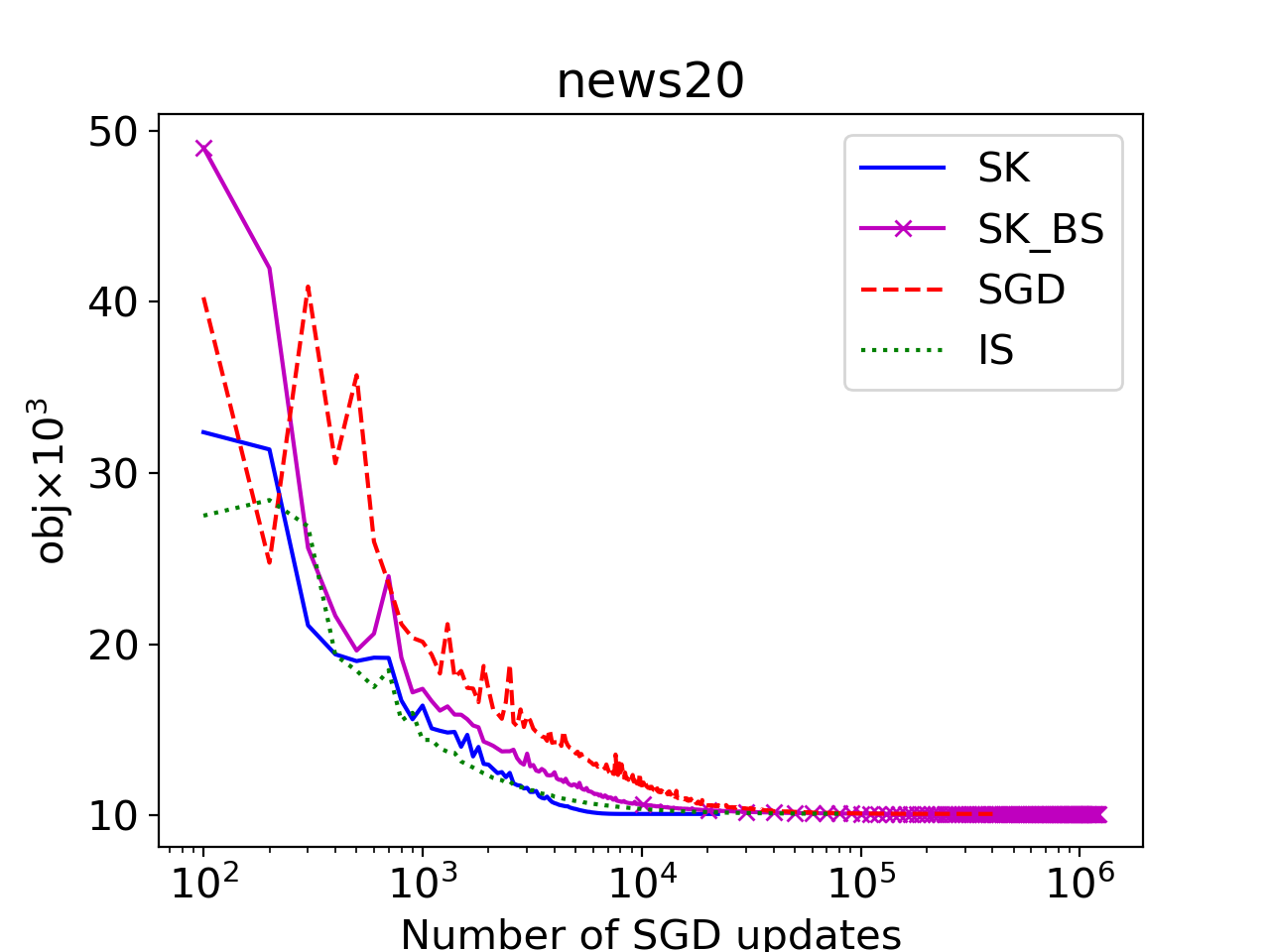
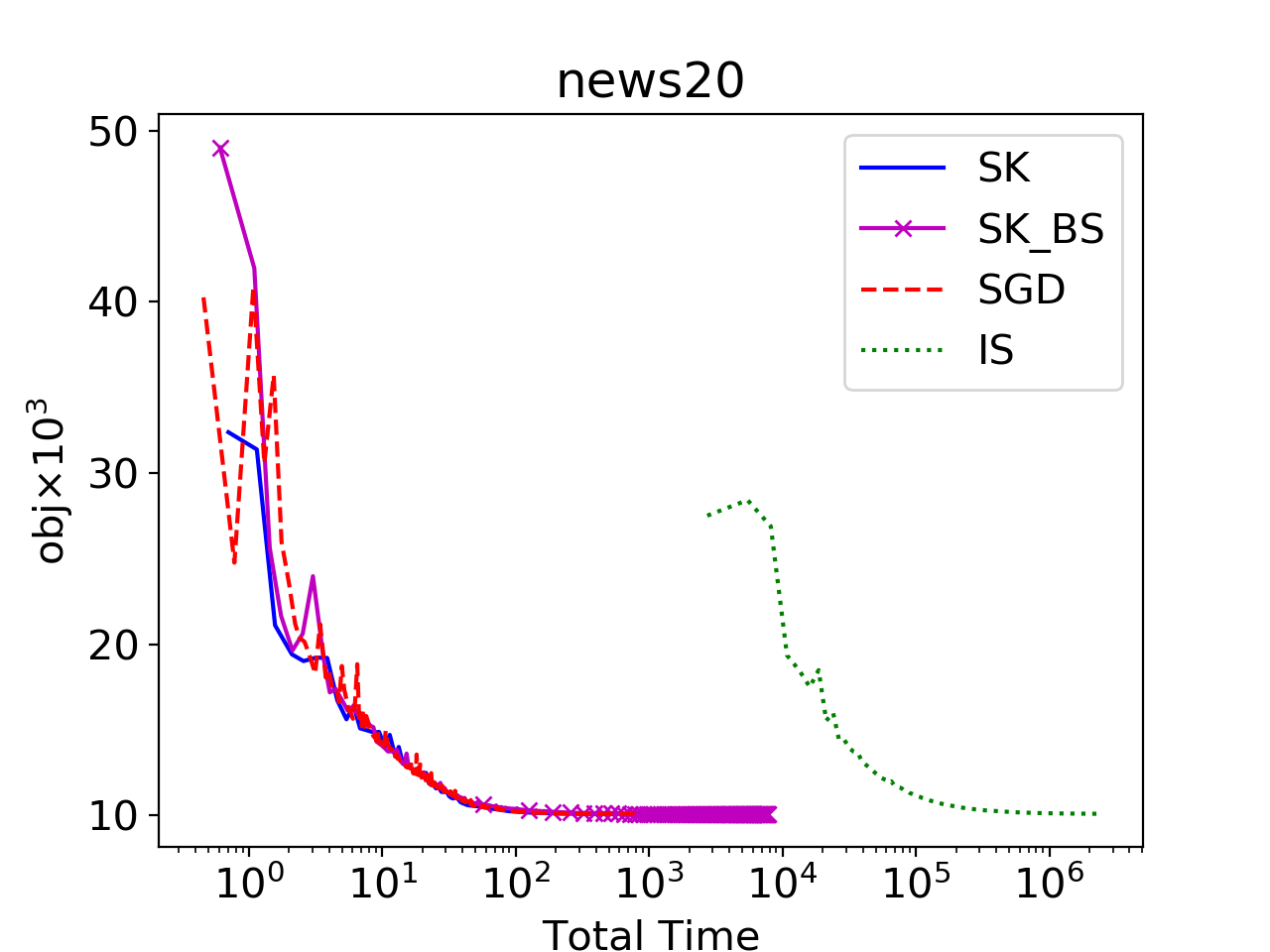
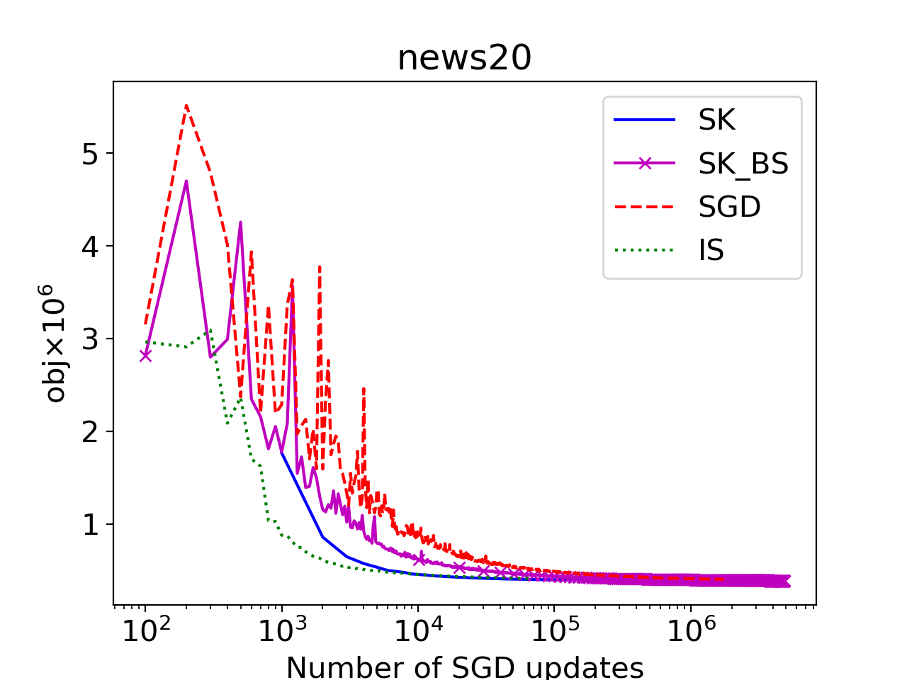
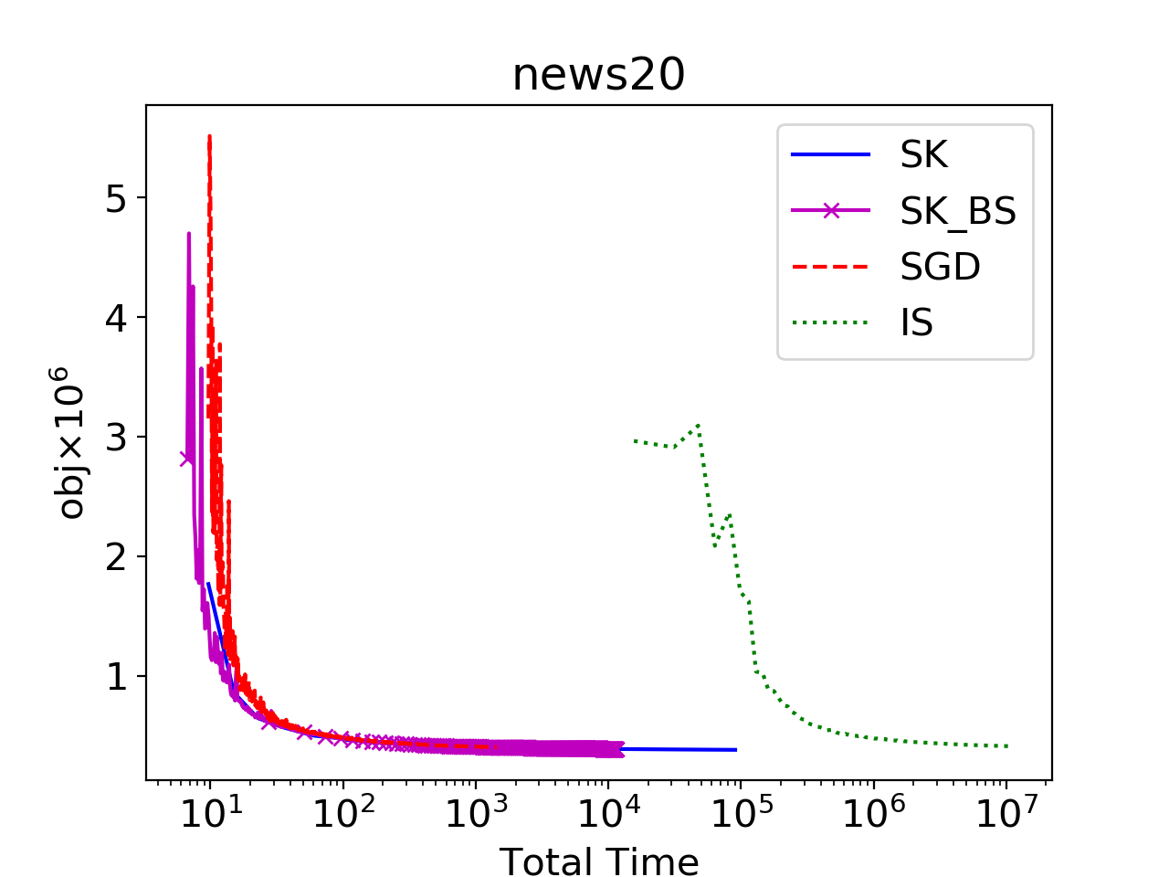
Figure 1: SVM on news20 and rcv1 datasets. In terms of the number of parameter updates, the shrinking method (SK), shrinking method with Bernoulli sampling (SK$\_$BS), and importance sampling (IS) methods have comparable performance, and are better than plain SGD. However, because of large computational overhead, importance sampling methods are not applicable to large datasets. In these experiments, per sample gradient magnitude is used as the importance weight distribution for importance sampling method and objective function value is used as shrinking criterion.

3.4 Shrinking experiment under convex setting

We test the shrinking algorithm on SVM binary classification tasks. The shrinking algorithm (SK) evaluates the objective function value upon receiving every randomly sampled training instance and deciding whether to take a training step on it. We compare shrinking (SK) with plain SGD and importance sampling (IS) algorithms as well as shrinking algorithm with Bernuli sampling (SK$\_$BS). In SK$\_$BS, different from hard shrinking (SK), one does not make immediate decision to ignore a certain instance but conduct a Bernuli sampling to make that decision; the detailed description can be found in Algorithm 1. The datasets are from libsvm [10, 5] and we implemented Pegasos [27] algorithm with C++ as the baseline method. All shrinking methods and importance sampling method achieve faster convergence compared with baseline SGD. However, because of the overhead to update importance weights, importance sampling method takes much more time to conduct same number of parameter updates, which makes it impractical for large datasets. Both shrinking methods have comparable time cost as baseline SGD and still have advantage over baseline SGD w.r.t. training time.

4 Theoretical Analysis

In this section, we establish the theoretical convergence of SGD with the proposed shrinking operations. It is easy to see that if certain instances are ignored during batch generation process, the stochastic gradients on that batch would be biased. Majority of the stochastic gradient methods try to build an unbiased estimator of the full gradient. Vanilla SGD achieves this through uniform sampling or random permutation. Importance sampling methods [15, 16] sample training batches based on importance weights. To ensure an unbiased stochastic gradient, an inverse weighted loss is typically used to replace the original loss in many importance sampling approaches. However, it is not necessary for an unbiased gradient estimate to be used to guarantee convergence of a stochastic gradient method. Many recent stochastic gradient algorithms are designed without using a unbiased gradient estimator, such as stochastic averaging gradients (SAG) [26] or asymptotic biased SGD [28]. Generally speaking, a SGD variant is able to converge as long as the difference between the used estimated gradient and the true gradient converges to zero. In Figure 1, we have observed that SGD with our proposed shrinking operations converges to the same objective function values as vanilla SGD for an L2-regularized linear SVM problem. We now theoretically prove that SGD with the proposed shrinking operation (8) is able to converge at $O(1/k)$ rate for $\mu$-strongly convex problems. In particular, with similar assumptions as used to establish convergence of vanilla SGD [4], let us consider a function $F({\bm{w}})$ that satisfies the following conditions:

Property 1.

$F({\bm{w}}):=\frac{1}{N}\sum_{i=1}^{N}f_{i}({\bm{w}})$ satisfies:

• $F$ is $\mu$-strongly convex,

• $\arg\min_{{\bm{w}}}F({\bm{w}})\in B_{D}=\mathopen{}\mathclose{{}\left\{{{\bm{w}}\mid\mathopen{}\mathclose{{}\left\|{{\bm{w}}}}\right\|\leq D}}\right\}$, and

• $\mathopen{}\mathclose{{}\left\|{\nabla f_{i}\mathopen{}\mathclose{{}\left({{\bm{w}}}}\right)}}\right\|\leq G,\ \forall{\bm{w}}\in B_{D}$

Note that the boundedness assumption is motivated from Pegasos [27], where a projection step is incorporated to limit the set of admissible solutions to a ball of radius $1/\mu$. In Theorem 1 (with similar assumptions as used to establish convergence of vanilla SGD [4]), we show that SGD with our proposed shrinking techniques converges for $\mu$-strongly convex problem with an $O(1/k)$ convergence rate.

Theorem 1.

Suppose function $F$ satisfies Property 1. For the stochastic gradient descent with the update rule ${\bm{w}}_{k+1}={\bm{w}}_{k}-\eta_{k}{\bm{g}}_{k}$, where step size $\eta_{k}=\frac{1}{\mu k}$ and stochastic gradient ${\bm{g}}_{k}$ is based on a uniformly randomly selected instance index $i$:

$${\bm{g}}_{k} =\nabla f_{i}({\bm{w}}_{k})-\bm{\epsilon}_{k},\ i\sim\mathtt{uniform}\mathopen{}\mathclose{{}\left({1,2,\ldots,N}}\right)$$ (9)

$$\bm{\epsilon}_{k} =\nabla f_{i}({\bm{w}}_{k})\mathbf{I}(\|\nabla f_{i}({\bm{w}}_{k})\|\leq\frac{G}{k})$$ (10)

we have

$$\mathds{E}(\|{\bm{w}}_{k}-{\bm{w}}^{*}\|^{2})\leq\frac{\max\mathopen{}\mathclose{{}\left(4D^{2},\frac{G^{2}}{\mu^{2}}+\frac{4DG}{\mu}}\right)}{k}$$ (11)

where $w^{*}$ is the optimal solution.

Proof of Theorem 1.

From strong convexity, we have:

$$F({\bm{w}}^{*})-F({\bm{w}}_{k})\geq\langle\nabla F({\bm{w}}_{k}),{\bm{w}}^{*}-{\bm{w}}_{k}\rangle+\frac{\mu}{2}\|{\bm{w}}_{k}-{\bm{w}}^{*}\|^{2}$$

$$F({\bm{w}}_{k})-F({\bm{w}}^{*})\geq\langle\nabla F({\bm{w}}^{*}),{\bm{w}}_{k}-{\bm{w}}^{*}\rangle+\frac{\mu}{2}\|{\bm{w}}_{k}-{\bm{w}}^{*}\|^{2}.$$

Adding the above inequalities gives:

$$\langle\nabla F({\bm{w}}_{k})-\nabla F({\bm{w}}^{*}),{\bm{w}}_{k}-{\bm{w}}^{*}\rangle \geq\mu\|{\bm{w}}_{k}-{\bm{w}}^{*}\|^{2}$$

$$\Rightarrow\quad\quad\quad\langle\nabla F({\bm{w}}_{k}),{\bm{w}}_{k}-{\bm{w}}^{*}\rangle \geq\mu\|{\bm{w}}_{k}-{\bm{w}}^{*}\|^{2}$$

$$\Rightarrow\ \quad\langle\mathbb{E}(\nabla f_{i}({\bm{w}}_{k})),{\bm{w}}_{k}-{\bm{w}}^{*}\rangle \geq\mu\|{\bm{w}}_{k}-{\bm{w}}^{*}\|^{2}$$ (12)

Next, we have:

$$\mathbb{E}(\|{\bm{w}}_{k+1}-{\bm{w}}^{*}\|^{2})=\mathbb{E}(\|{\bm{w}}_{k}-\eta_{k}{\bm{g}}_{k}-{\bm{w}}^{*}\|^{2})$$

$$= \mathbb{E}(\|{\bm{w}}_{k}-{\bm{w}}^{*}\|^{2})-2\eta_{k}\mathbb{E}\langle{\bm{g}}_{k},{\bm{w}}_{k}-{\bm{w}}^{*}\rangle+\eta_{k}^{2}\mathbb{E}(\|{\bm{g}}_{k}\|^{2})$$

$$\leq \mathbb{E}(\|{\bm{w}}_{k}-{\bm{w}}^{*}\|^{2})-2\eta_{k}\mathbb{E}\langle\nabla f_{i}({\bm{w}}_{k}),{\bm{w}}_{k}-{\bm{w}}^{*}\rangle$$

$$+\eta_{k}^{2}G^{2}+2\eta_{k}\mathbb{E}\langle\bm{\epsilon}_{k},{\bm{w}}_{k}-{\bm{w}}^{*}\rangle$$ (13)

The last term from (13) can be upper bounded as follows:

$$2\eta_{k}\mathbb{E}\langle\bm{\epsilon}_{k},{\bm{w}}_{k}-{\bm{w}}^{*}\rangle$$

$$= 2\eta_{k}\mathbb{E}\mathopen{}\mathclose{{}\left(\langle\nabla f_{i}({\bm{w}}_{k}),{\bm{w}}_{k}-{\bm{w}}^{*}\rangle\mathbf{I}\mathopen{}\mathclose{{}\left(\|\nabla f_{i}({\bm{w}}_{k})\|\leq\frac{G}{k}}\right)}\right)$$

$$\leq 2\eta_{k}\mathbb{E}\mathopen{}\mathclose{{}\left(\|\nabla f_{i}({\bm{w}}_{k})\|\|{\bm{w}}_{k}-{\bm{w}}^{*}\|\mathbf{I}\mathopen{}\mathclose{{}\left(\|\nabla f_{i}({\bm{w}}_{k})\|\leq\frac{G}{k}}\right)}\right)$$

$$\leq 2\eta_{k}\frac{2DG}{k}$$ (14)

Substituting (12) and (14) into (13), we have:

$$\mathbb{E}(\|{\bm{w}}_{k+1}-{\bm{w}}^{*}\|^{2})=\mathbb{E}(\|{\bm{w}}_{k}-\eta_{k}{\bm{g}}_{k}-{\bm{w}}^{*}\|^{2})$$

$$\leq \mathbb{E}(\|{\bm{w}}_{k}-{\bm{w}}^{*}\|^{2})(1-\frac{2}{k})+\mathopen{}\mathclose{{}\left(\frac{4DG}{\mu}+\frac{G^{2}}{\mu^{2}}}\right)\frac{1}{k^{2}}$$ (15)

Let $L=\max(\|{\bm{w}}_{1}-{\bm{w}}^{*}\|,\frac{G^{2}+4DG\mu}{\mu^{2}})$, the $O(1/k)$ convergence (11) can be established by induction. When $k=1$, the result holds:

$$\mathbb{E}(\|{\bm{w}}_{1}-{\bm{w}}^{*}\|^{2})\leq\frac{\max\mathopen{}\mathclose{{}\left(4D^{2},\frac{G^{2}}{\mu^{2}}+\frac{4DG}{\mu}}\right)}{1}$$ (16)

Suppose the result holds for $k$, then for $k+1$:

$$\mathbb{E}(\|{\bm{w}}_{k+1}-{\bm{w}}^{*}\|^{2})=\mathbb{E}(\|{\bm{w}}_{k+1}-\eta_{k}{\bm{g}}_{k}-{\bm{w}}^{*}\|^{2})$$

$$\leq \mathopen{}\mathclose{{}\left(1-\frac{2}{k}}\right)\frac{L}{k}+L\frac{1}{k^{2}}=\frac{k-1}{k^{2}}L\leq\frac{L}{k+1}$$ (17)

 

Theorem 1 indicates that in the strongly convex case, shrinking based on gradient magnitude is able to achieve the same convergence as SGD even though the stochastic gradient is biased. For many ML models, computation of objective function value is cheaper than computation of gradients. Also, for $\mu$-strongly convex $F({\bm{w}})$ which is $M$-Lipschitz smooth we have:

$$\|\nabla F({\bm{w}})-\nabla F({\bm{w}}^{*})\|^{2} =\|\nabla F({\bm{w}})\|^{2}\leq M^{2}\|{\bm{w}}-{\bm{w}}^{*}\|^{2}$$

$$F({\bm{w}})-F({\bm{w}}^{*}) \geq\frac{\mu}{2}\|{\bm{w}}-{\bm{w}}^{*}\|^{2}$$

Thus, gradient magnitude and objective function value is the same in terms of measuring instance triviality:

$$\mu(F({\bm{w}})-F({\bm{w}}^{*}))\leq\frac{1}{2}\|\nabla F({\bm{w}})\|^{2}\leq\frac{M^{2}}{\mu}(F({\bm{w}})-F({\bm{w}}^{*}))$$

where the left inequality is the Polyak-Lojasiewicz inequality. Due to these reasons, in practice we can usually use the loss function value as the shrinking criterion.

5 AutoAssist: Learning with an Assistant

The goal of instance shrinking is to reduce the model training time, especially for tasks with large number of instances and complex models such as deep learning. Although the shrinking method is able to greatly reduce the number of updates needed to converge, the improvement is not that obvious in terms of training time. The reason is that we need almost the same amount of computation to decide whether to ignore an instance as to conduct the gradient update. Thus the reduced time for parameter updating is compensated by the overhead introduced by the decision procedure for shrinking. To reduce such overhead, we need to have a cheaper way to make shrinking decisions. Specifically for deep learning, using a light weight model for instance shrinking can save us a lot of computation. In this section, we propose a training framework, named AutoAssist, that trains a light weight model to make the shrinking decision for deep learning models.

5.1 Assistant for instance selection

In many machine learning applications, it is observed that data that follows a certain pattern can be better handled than others. For example, in image classification tasks, at a certain training phase, a shirt and a pair of jeans may be well distinguished, but a pair of shorts may be confused with a pair of jeans. Also, in machine translation tasks, sentences containing certain ambiguous tokens may not be translated well, while those with precise meanings may be handled very well. Many such patterns can be learned through very simple models, such as a shallow convolutional network or a bag-of-words classifier. Motivated by these observations, we propose to attach a light-weight model (Assistant) to the major deep neural network (Boss) to assist the Boss with selecting informative training instances.

The traditional deep learning training pipeline includes two major parts: the batch generator (BG) and the forward propagation (FP) / backward propagation (BP) machine. A vanilla batch generator iterates through the whole dataset which is randomly permuted after each epoch. In the AutoAssist training framework, a Boss (FP/BP machine) and an Assistant (machine learned batch generator) work together. The Assistant is constructed such that it can (1) choose training batches cleverly to boost Boss training while (2) introducing low overhead. To resolve (1) we let the Assistant learn from the performance of the Boss on different examples and generate most informative training batch at each training stage. Also, because of the design of AutoAssist, it is possible to use a CPU/GPU parallel learning scheme that minimizes Assistant overhead to Boss.

5.2 Learning to generate smart training batches

The ideal Assistant would evolve with the Boss and make accurate selections based on the latest behavior of the Boss. At the beginning of training, the Assistant presents easy examples to Boss in order to get better convergence. As boss converges, the easy instances become less and less informative and the Assistant gradually decreases the presentation ratio of easy instances and increases the difficulty of instances in the batch according to the ability of Boss to handle them. Specifically, we design the Assistant network ($g(\cdot)$) to be a classifier parameterized by $\bm{\phi}$ that tries to predict the difficulty of instances by minimizing:

$$\min_{\bm{\phi}}\frac{1}{N}\sum_{i=0}^{N}\hat{L}(g({\bm{x}}_{i},{\bm{y}}_{i},\bm{\phi}),z_{i})$$ (18)

where $\hat{L}$ is the cross entropy loss and $z_{i}$ is the binary label indicating if this is a trivial instance. One possible definition of $z_{i}$ is:

$$z_{i}=\mathopen{}\mathclose{{}\left\{\begin{array}[]{ll}1&,\;\;\;f({\bm{x}}_{i},{\bm{y}}_{i},\bm{\theta})>T\\ 0&,\;\;\;{\mbox{\rm otherwise}}.\end{array}}\right.$$

where $T$ is the threshold for instance shrinking and $f({\bm{x}},{\bm{y}},\bm{\theta})$ is the objective function value of the Boss network parameterized by $\bm{\theta}$. By jointly learning Boss and Assistant, we can guarantee that the Assistant network is trained on the latest labels, i.e. the $z_{i}$’s generated by the latest Boss model $f({\bm{x}}_{i},{\bm{y}}_{i},\bm{\theta})$. The training batch $B\subset[N]$ is then generated via a series of Bernoulli samplings with a smoothing term $\gamma$.

• Input: Training dataset $D=\{{\bm{x}}_{i},{\bm{y}}_{i}\}_{i=1}^{N}$, base probability $\gamma$

• Output: sampled batch index $B\subset[N]$

• Initialize: $B=[]$

• While $B$.size() $<$ batch$\_$size:

  • $idx\sim\texttt{uniformInt}(N)$

  • $c\sim\texttt{uniform}(0,1)$

  • If $c<\gamma$:

    • B.append($idx$)

  • Else:

    • $\hat{c}=\frac{c-\gamma}{1-\gamma}$ // another uniform(0,1) variable

    • If $\hat{c}<g({\bm{x}}_{i},{\bm{y}}_{i},\bm{\phi})$:

      • B.append($idx$)

• Return $B$

Algorithm 1 Assistant.sample$\_$batch

Noting that $p_{i}$ and $\frac{p_{i}-\gamma}{1-\gamma}$ are independent variables, we only need to evaluate $g_{i}$ upon receiving a random sampled index $i$. In practice, index $i$ loops over the randomly shuffled training data index list rather than sampled uniformly. Thus a well-trained Assistant will save us a lot of computation time by skipping trivial instances, thus accelerating convergence. Usually the Assistant model is chosen to be light weight and may share knowledge from the Boss. For example, in image classification tasks, the Assistant may be constructed as a convolution layer followed by a pooling layer and a single linear layer, where the convolution layer shares parameter s with the Boss.

5.3 Asynchronous joint learning with CPU/GPU

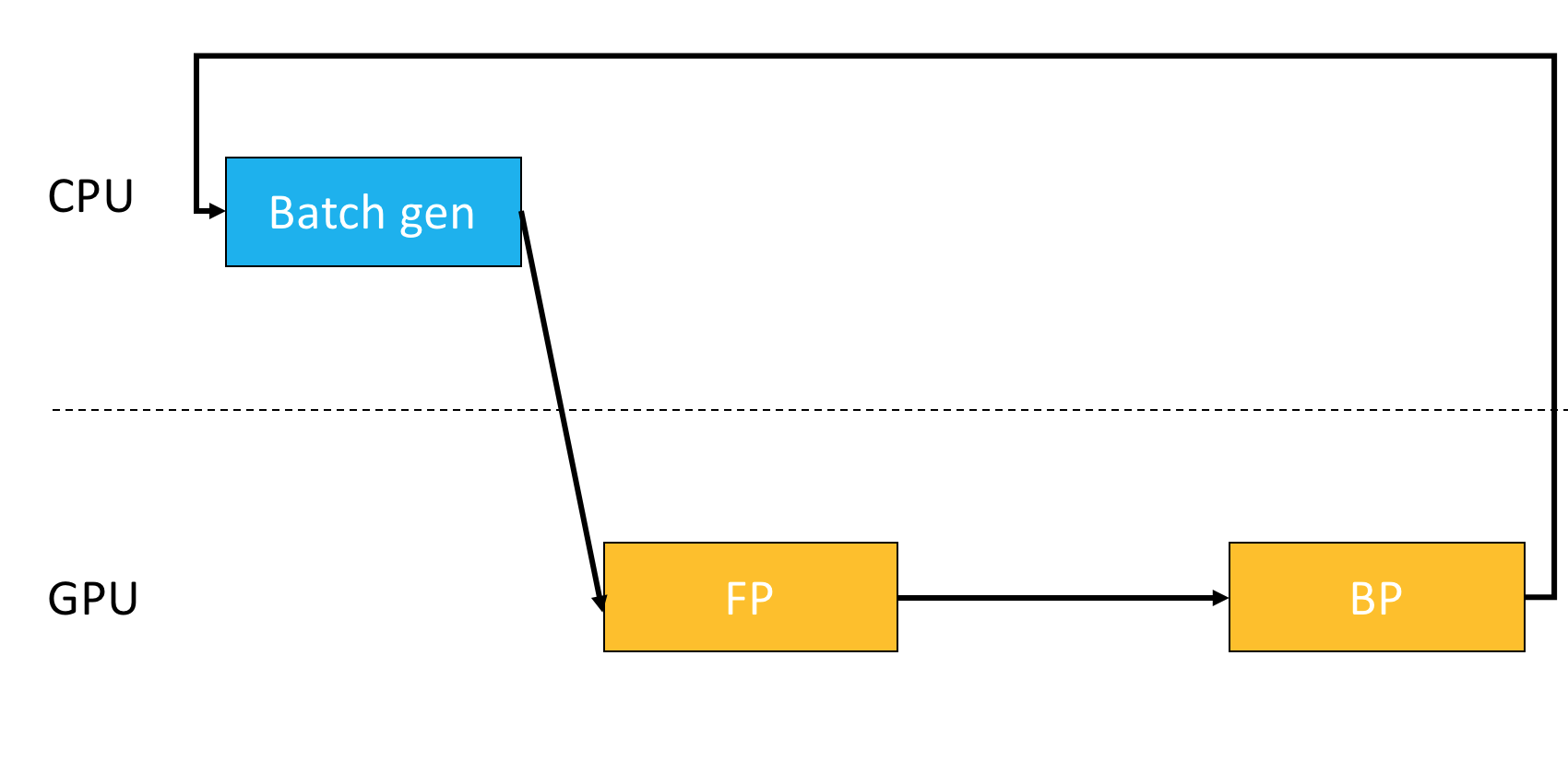
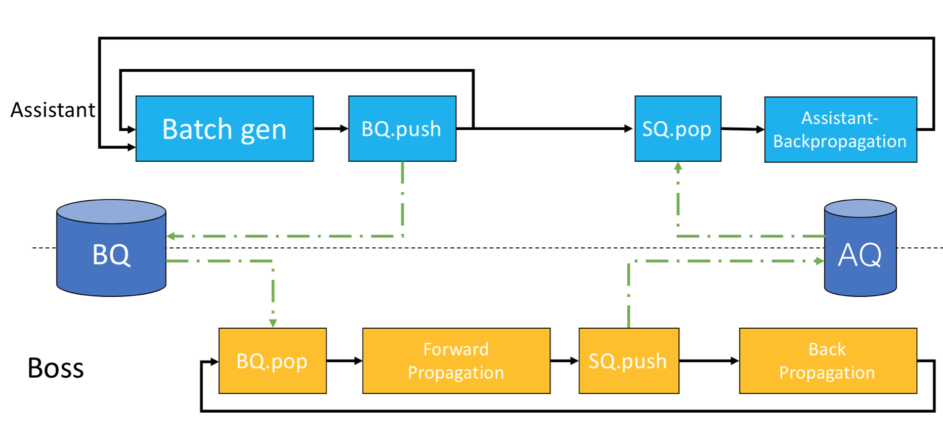
Figure 2: The computation scheme of vanilla training on the left wastes CPU/GPU cycles, while the accelerated training process with AutoAssist trains both the Boss and the Assistant asynchronously.

Another concern is the concept that a good Assistant will best utilize the time schedule of Boss. That is we want the Assistant network to introduce as little overhead to the training of the Boss network as possible. In traditional mini-batch training of deep networks, the batch generation on CPU and training on GPU are done sequentially. Thus at least one of the CPU/GPU is idle at each moment during training. In our AutoAssist framework, we propose a training algorithm where both the CPU and GPU work asynchronously on their jobs. This reduces the overhead of batch generation or Assistant training to GPU time and could potentially be generalized to multi-CPU setting. Specifically, we maintain two queues of mini-batches:

BossQueue $$=\{\{{\bm{x}}_{i},{\bm{y}}_{i}\},\ldots\}$$ (19)

AssistantQueue $$=\{\{i,f({\bm{x}}_{i},{\bm{y}}_{i},\bm{\theta})\},\ldots\}$$ (20)

During each mini-batch training step, Boss obtains a batch of instances $\{{\bm{x}}_{i},{\bm{y}}_{i}\}_{i\in B}$ from BossQueue (BQ) and conducts the forward propagation on $B$ to obtain losses $\{f({\bm{x}}_{i},{\bm{y}}_{i},\bm{\theta})\}$. Then the Boss pushes the index-loss pairs $\{i,f({\bm{x}}_{i},{\bm{y}}_{i},\bm{\theta})\}_{i\in B}$ to AssistantQueue (AQ). Assistant on the other hand, trains on items from AssistantQueue and sample training batch and push to BossQueue. In most cases, the training step of Boss is much more expensive than that of Assistant thus it is easy for Assistant to keep BossQueue non-empty at all times. The only overhead on Boss’s timeline is pushing the loss information to AQ, which is minimal work considering that each instance only consists of two scalars (index, loss).

6 Experimental results

In this section we present the experimental results. We tested the AutoAssist model on two different tasks: image classification and neural machine translation. All experiments are done on Tesla V100 GPUs with implementation in PyTorch [25].

6.1 Image classification

We tested our models on MNIST [22] hand written digit dataset, FashionMNIST [30] fashion item image dataset, Extended MNIST [7] and CIFAR10 [19] datasets. A logistic regression model is used as the Assistant network and ResNet [11] as the Boss network. AutoAssist is constructed to optimize the binary classification objective (18). Adam [18] is used as the optimizer for all models.

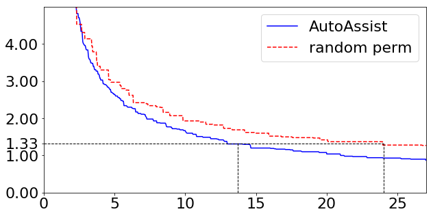
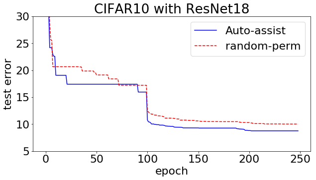
Figure 3: Test accuracy on MNIST and CIFAR10 datasets — to reach error 1.33 on MNIST, AutoAssist needs only about half the number of epochs as random permutation.

Adding Auto-assist is able to improve the final test accuracy on MNIST and CIFAR10 datasets and enables faster convergence. On the MNIST dataset, to achieve $98.67\%$ test accuracy, the baseline approach takes 24 epochs through the entire data, while it takes Auto-assist just 13.7 epochs to achieve similar accuracy. On other image classification datasets, AutoAssist is also able to improve the final test accuracy.

Data	random-perm	AutoAssist
MNIST	98.67	99.17
FashionMNIST	90.68	90.99
ExtendedMNIST	87.21	87.28
CIFAR10	90.04	90.23

Table 1: Accuracy with/without Assistant.

6.2 Machine Translation

For machine translation tasks, we tested our AutoAssist model with two translation datasets: the English-German Image Description dataset [9] and WMT 2014 English-German dataset. The Boss model is chosen to be the transformer model [29] and the Assistant is chosen to be a bag of word classifier. For the smaller dataset Multi30K, which consists of around 30k language pairs, we train the transformer base model on a single GPU machine and used batch size of 64 sentences. Besides the vanilla random shuffling batch generation method, we also compared with the self-paced-learning (SPL) algorithm [20, 23] and choose the best pace step $q(t)$ over multiple tests.

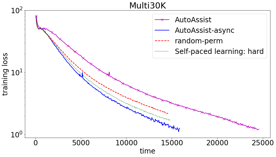
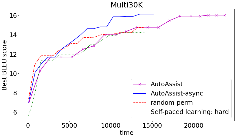
Figure 4: The training error and BLEU score on Multi30k dataset. AutoAssist with CPU/GPU asynchronous training converges faster and achieves higher BLEU score.

Table 2 shows the time required to complete one epoch on the Multi30k dataset. With the proposed asynchronous training pipeline, the time overhead introduced by AutoAssist is only $5\%$ while the sequential implementation has $61\%$ overhead.

Model	sentence-pairs/second
baseline	617.3
AutoAssist	382.7
AutoAssist-async	586.0

Table 2: Number of sentence pairs trained per second. CPU/GPU asynchronous training is able to decrease $92\%$ of the time overhead.

On the WMT 2014 English to German dataset consisting of about 4.5 million sentence pairs, we trained the transformer model with the base setting in [29] and constructed source vocabulary and target vocabulary of size 40k and 43k respectively. Both vanilla and AutoAssist models are trained on 8 Tesla V100 GPUs with around 40k tokens per training batch (5k tokens per batch per GPU). For the vanilla model, batches are pre-generated and randomly shuffled at the beginning of each epoch. For the AutoAssist model, data are split into 8 chunks with the same number of tokens and 8 Assistant models are trained simultaneously to generate batches for each GPU. Each Assistant will thus be trained on a subset of the data and generate training batch from that chunk of data. We generate translation results with beam size of 4 and length penalty of 0.6. We are able to obtain 27.1 BLEU score with both the vanilla and AutoAssist model.s The AutoAssist is able to achieve higher BLEU score with fewer tokens seen. For example, the vanilla model reaches BLEU score of 26 after training on 1.82 billion tokens while the AutoAssist only needs 1.18 billion tokens. This means that the instances the Assistant decides to ignore have little contribution to the convergence and thus can be ignored with no harm.

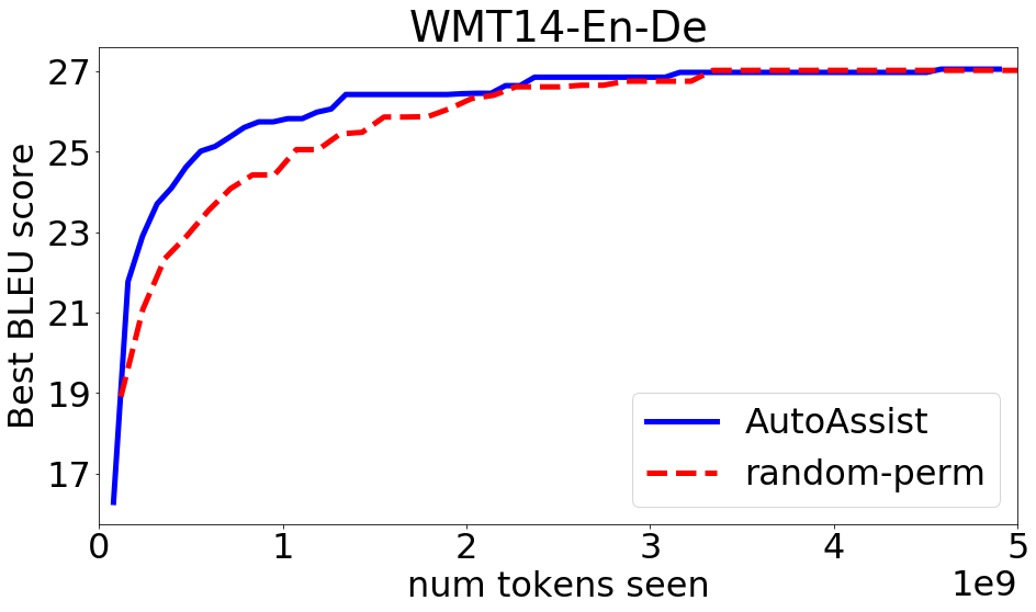
Figure 5: BLEU score on WMT14 En-De dataset

Model	vanilla	Auto-assist
avr $\#$ tokens per epoch	12.1M	7.87M
BLEU reach 26	$1.82\times 10^{9}$	1.18$\times 10^{9}$
BLEU reach 27	$3.22\times 10^{9}$	3.01$\times 10^{9}$

Table 3: Number of tokens needed to reach different BLEU score level. AutoAssist is able to save $35\%$ tokens to reach 26 and $6\%$ to reach 27.

7 Conclusions

In this paper, motivated by the dual coordinate shrinking method in SVM dual coordinate descent, we propose a training framework to accelerate deep learning model training. The proposed framework, Auto-assist, jointly trains a batch generator (Assistant) along with the main deep learning model (Boss). The Assistant model conducts primal instance shrinking to get rid of trivial instances during training and can automatically adjust the criteria based on the ability of the Boss. In the strongly convex setting, even though our method leads to biased gradients, we should that stochastic gradient with instance shrinking has $O(\frac{1}{k})$ convergence, which is the same as plain SGD. To maximize the training efficiency of CPU/GPU cycles, we let the Assistant learn from the output of the Boss in an asynchronous parallel scheme. We further propose a method to reduce the computational overhead by training Assistant and Boss asynchronously on CPU/GPU. Experiments show that both convergence and accuracy could be improved through introducing our Assistant model. The CPU/GPU asynchronous training pipeline is able to reduce the overhead to less than $10\%$ compared with the sequential pipeline.

Appendix A Algorithms for CPU/GPU parallelization

• Input: Training dataset $D=\{{\bm{x}}_{i},{\bm{y}}_{i}\}_{i=1}^{N}$

• Initialize: BossQueue, AssistantQueue, Assistant

• While True:

  • If BossQueue.size()$<k$:

    • B = Assistant.sample$\_$batch()

    • BossQueue.enqueue(B)

  • Else if not AssistantQueue.empty():

    • M= AssistantQueue.pop()

    • grad = Assistant.gradient(M)

    • Assistant.update(grad)

Algorithm 2 algorithm for assistant (CPU)

• Input:

• Initialize: Boss

• While True:

  • If not BossQueue.empty():

    • B = BossQueue.pop()

    • M = Boss.Forward(B)

    • AssistantQueue.enqueu(M)

    • grad = Boss.Backward(M)

    • Boss.update(grad)

Algorithm 3 algorithm for Boss (GPU)

References

- [1] Guillaume Alain, Alex Lamb, Chinnadhurai Sankar, Aaron Courville, and Yoshua Bengio. Variance reduction in sgd by distributed importance sampling. arXiv preprint arXiv:1511.06481, 2015.
- [2] Samy Bengio, Oriol Vinyals, Navdeep Jaitly, and Noam Shazeer. Scheduled sampling for sequence prediction with recurrent neural networks. In Advances in Neural Information Processing Systems, pages 1171–1179, 2015.
- [3] Yoshua Bengio, Jérôme Louradour, Ronan Collobert, and Jason Weston. Curriculum learning. In Proceedings of the 26th annual international conference on machine learning, pages 41–48. ACM, 2009.
- [4] Léon Bottou, Frank E Curtis, and Jorge Nocedal. Optimization methods for large-scale machine learning. SIAM Review, 60(2):223–311, 2018.
- [5] Chih-Chung Chang and Chih-Jen Lin. LIBSVM: A library for support vector machines. ACM Transactions on Intelligent Systems and Technology, 2:27:1–27:27, 2011. Software available at http://www.csie.ntu.edu.tw/~cjlin/libsvm.
- [6] Haw-Shiuan Chang, Erik Learned-Miller, and Andrew McCallum. Active bias: Training more accurate neural networks by emphasizing high variance samples. In Advances in Neural Information Processing Systems, pages 1002–1012, 2017.
- [7] Gregory Cohen, Saeed Afshar, Jonathan Tapson, and André van Schaik. EMNIST: an extension of MNIST to handwritten letters. arXiv preprint arXiv:1702.05373, 2017.
- [8] Ronan Collobert and Jason Weston. A unified architecture for natural language processing: Deep neural networks with multitask learning. In Proceedings of the 25th international conference on Machine learning, pages 160–167. ACM, 2008.
- [9] D. Elliott, S. Frank, K. Sima’an, and L. Specia. Multi30k: Multilingual english-german image descriptions. pages 70–74, 2016.
- [10] Rong-En Fan, Kai-Wei Chang, Cho-Jui Hsieh, Xiang-Rui Wang, and Chih-Jen Lin. LIBLINEAR: A library for large linear classification. Journal of Machine Learning Research, 9:1871–1874, 2008.
- [11] Kaiming He, Xiangyu Zhang, Shaoqing Ren, and Jian Sun. Deep residual learning for image recognition. In Proceedings of the IEEE conference on computer vision and pattern recognition, pages 770–778, 2016.
- [12] Cho-Jui Hsieh, Kai-Wei Chang, Chih-Jen Lin, S Sathiya Keerthi, and Sellamanickam Sundararajan. A dual coordinate descent method for large-scale linear svm. In Proceedings of the 25th international conference on Machine learning, pages 408–415. ACM, 2008.
- [13] Lu Jiang, Deyu Meng, Qian Zhao, Shiguang Shan, and Alexander G Hauptmann. Self-paced curriculum learning. In AAAI., page Vol. 2. No. 5.4., 2015.
- [14] Lu Jiang, Zhengyuan Zhou, Thomas Leung, Li-Jia Li, and Li Fei-Fei. Mentornet: Learning data-driven curriculum for very deep neural networks on corrupted labels. arXiv preprint arXiv:1712.05055, 2017.
- [15] Angelos Katharopoulos and François Fleuret. Biased importance sampling for deep neural network training. arXiv preprint arXiv:1706.00043, 2017.
- [16] Angelos Katharopoulos and François Fleuret. Not all samples are created equal: Deep learning with importance sampling. arXiv preprint arXiv:1803.00942, 2018.
- [17] Tae-Hoon Kim and Jonghyun Choi. Screenernet: Learning curriculum for neural networks. arXiv preprint arXiv:1801.00904, 2018.
- [18] Diederik P Kingma and Jimmy Ba. Adam: A method for stochastic optimization. arXiv preprint arXiv:1412.6980, 2014.
- [19] Alex Krizhevsky. Learning multiple layers of features from tiny images. Technical report, Citeseer, 2009.
- [20] M Pawan Kumar, Benjamin Packer, and Daphne Koller. Self-paced learning for latent variable models. In Advances in Neural Information Processing Systems, pages 1189–1197, 2010.
- [21] Martin Längkvist, Lars Karlsson, and Amy Loutfi. A review of unsupervised feature learning and deep learning for time-series modeling. Pattern Recognition Letters, 42:11–24, 2014.
- [22] Yann LeCun and Corinna Cortes. MNIST handwritten digit database. 2010.
- [23] Hao Li and Maoguo Gong. Self-paced convolutional neural networks. In Proceedings of the International Joint Conference on Artificial Intelligence, 2017.
- [24] Deanna Needell, Rachel Ward, and Nati Srebro. Stochastic gradient descent, weighted sampling, and the randomized kaczmarz algorithm. In Advances in Neural Information Processing Systems, pages 1017–1025, 2014.
- [25] Adam Paszke, Sam Gross, Soumith Chintala, Gregory Chanan, Edward Yang, Zachary DeVito, Zeming Lin, Alban Desmaison, Luca Antiga, and Adam Lerer. Automatic differentiation in PyTorch. 2017.
- [26] Mark Schmidt, Nicolas Le Roux, and Francis Bach. Minimizing finite sums with the stochastic average gradient. Mathematical Programming, 162(1-2):83–112, 2017.
- [27] Shai Shalev-Shwartz, Yoram Singer, Nathan Srebro, and Andrew Cotter. Pegasos: Primal estimated sub-gradient solver for svm. Mathematical programming, 127(1):3–30, 2011.
- [28] Vladislav B Tadić, Arnaud Doucet, et al. Asymptotic bias of stochastic gradient search. The Annals of Applied Probability, 27(6):3255–3304, 2017.
- [29] Ashish Vaswani, Noam Shazeer, Niki Parmar, Jakob Uszkoreit, Llion Jones, Aidan N Gomez, Łukasz Kaiser, and Illia Polosukhin. Attention is all you need. In Advances in Neural Information Processing Systems, pages 5998–6008, 2017.
- [30] Han Xiao, Kashif Rasul, and Roland Vollgraf. Fashion-MNIST: a novel image dataset for benchmarking machine learning algorithms. arXiv preprint arXiv:1708.07747, 2017.
- [31] Peilin Zhao and Tong Zhang. Stochastic optimization with importance sampling for regularized loss minimization. In international conference on machine learning, pages 1–9, 2015.