Renormalization in the Golden-Mean Semi-Siegel Hénon Family: Non-Quasisymmetry

Abstract.

For quadratic polynomials of one complex variable, the boundary of the golden-mean Siegel disk must be a quasicircle. We show that the analogous statement is not true for quadratic Hénon maps of two complex variables.

1. Introduction

Let $\theta\in({\mathbb{R}}\setminus{\mathbb{Q}})/{\mathbb{Z}}$ be an irrational rotation number. Then $\theta$ can be represented by an infinite continued fraction:

$$\theta=[a_{0},a_{1},\ldots{}]=\cfrac{1}{a_{0}+\cfrac{1}{a_{1}+\cfrac{1}{a_{2}+\ldots{}}}}.$$

The $n$th partial convergent of $\theta$ is the rational number

$$\frac{p_{n}}{q_{n}}=[a_{0},a_{1},\ldots,a_{n}].$$

The denominator $q_{n}$ is called the $n$th closest return moment. The sequence $\{q_{n}\}_{n=0}^{\infty}$ satisfy the following inductive relation:

$$q_{0}=1\hskip 14.22636pt,\hskip 14.22636ptq_{1}=a_{0}\hskip 14.22636pt\text{and}\hskip 14.22636ptq_{n+1}=a_{n}q_{n}+q_{n-1}\hskip 14.22636pt\text{for}\hskip 14.22636ptn\geq 1.$$

We say that $\theta$ is Diophantine of order $d$ if there exists $C>0$ such that

$$q_{n+1}<Cq_{n}^{d-1}\hskip 14.22636pt\text{for all}\hskip 14.22636ptn\in\mathbb{N}$$

If $\theta$ is Diophantine of order $2$, then $\theta$ is said to be of bounded type. It is easy to show that $\theta$ is of bounded type if and only if $a_{n}$’s are uniformly bounded (see e.g. [M]). The simplest example of a bounded type rotation number is the inverse-golden mean:

$$\theta_{*}=\frac{\sqrt{5}-1}{2}=[1,1,\ldots].$$

Observe that for $\theta_{*}$, the sequence of closest return moments $\{q_{n}\}_{n=0}^{\infty}$ is the Fibonacci sequence.

Consider the standard one-parameter family of quadratic polynomials

$$f_{c}(z):=z^{2}+c\hskip 14.22636pt\text{for }c\in{\mathbb{C}}.$$

This is referred to as the quadratic family. A quadratic polynomial $f_{c}$ is determined uniquely by the multiplier $\mu\in{\mathbb{C}}$ at a fixed point $x_{c}\in{\mathbb{C}}$ for $f_{c}$. In fact, we have

$$c=\frac{\mu}{2}-\frac{\mu^{2}}{4}.$$ (1.1)

Let $c_{0}$ be the unique parameter such that for $f_{c_{0}}$, the fixed point $x_{c_{0}}$ is irrationally indifferent with rotation number $\theta$ (i.e. $\mu=e^{2\pi i\theta}$). If $\theta$ is equal to the inverse golden-mean $\theta_{*}$, then we denote $f_{c_{0}}$ as simply $f_{*}$.

The quadratic polynomial $f_{c_{0}}$ is said to be Siegel if it is locally linearizable at $x_{0}$. More precisely, $f_{c_{0}}$ is Siegel if there exist neighborhoods $U$ of $0$ and $V$ of $x_{0}$, and a biholomorphic change of coordinates

$$\psi:(U,0)\to(V,x_{0})$$

such that

$$\psi^{-1}\circ f_{c_{0}}\circ\psi(z)=\mu z.$$

A classic theorem of Siegel states, in particular, that $f_{c_{0}}$ is Siegel whenever $\theta$ is Diophantine. Moreover, it is known that the linearizing map $\psi$ can be biholomorphically extended to a map $\psi:(\mathbb{D},0)\rightarrow(\Delta,x_{0})$ so that its image $\Delta:=\psi(\mathbb{D})$ is maximal (see e.g. [M]). We call $\Delta$ and $\partial\Delta$ the Siegel disk and the Siegel boundary of $f_{c_{0}}$ respectively. See Figure 1.

It is natural to ask whether $\partial\Delta$ is a Jordan curve, and if so, whether it is quasisymmetric, or even smooth. The following theorem settles these questions in the case when $\theta$ is of bounded type (see [He]):

Theorem 1.1 (Douady, Ghys, Herman, Shishikura).

Suppose that $\theta$ is of bounded type. Then $f_{c_{0}}$ has its critical point $0$ on its Siegel boundary $\partial\Delta$, and the restriction $f_{c_{0}}|_{\partial\Delta}:\partial\Delta\to\partial\Delta$ is quasisymmetrically conjugate to the rigid rotation of the unit circle $\partial\mathbb{D}$ by $\theta$.

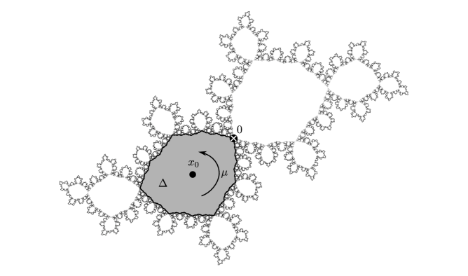
Figure 1. The Siegel disk $\Delta$ of the golden-mean Siegel quadratic polynomial $f_{*}$. The critical point $0$ is on $\partial\Delta$, and the restriction $f_{*}|_{\partial\Delta}:\partial\Delta\to\partial\Delta$ is quasisymmetrically conjugate to the rigid rotation of the unit circle $\partial\mathbb{D}$ by the angle $\theta_{*}=(\sqrt{5}-1)/2$.

From Theorem 1.1, it immediately follows that $\partial\Delta$ cannot be smooth if $\theta$ is of bounded type, since any curve containing the critical point cannot be both invariant and smooth. It is important to note, however, that there are examples of quadratic Siegel polynomials for which the Siegel boundary does not contain the critical point and is in fact smooth (see [BuCh]).

The main goal of this paper is to carry the study of Siegel boundaries to a higher dimensional setting. To this end, consider the following two-dimensional extension of the quadratic family:

$$H_{c,b}(x,y):=(x^{2}+c-by,x)\hskip 14.22636pt\text{for }c\in{\mathbb{C}}\text{ and }b\in{\mathbb{C}}\setminus\{0\}.$$

This is referred to as the (complex quadratic) Hénon family.

It is easy to see that $H_{c,b}$ has constant Jacobian:

$$\text{Jac}\,H_{c,b}\equiv b.$$

Moreover, for $b=0$, the map $H_{c,b}$ degenerates to the following embedding of $f_{c}$:

$$\iota(f_{c})(x,y):=(f_{c}(x),x).$$

Hence, the parameter $b$ measures how far $H_{c,b}$ is from being a degenerate one-dimensional system. In this paper, we will always assume that $H_{c,b}$ is a dissipative map (i.e. $|b|<1$).

A Hénon map $H_{c,b}$ is determined uniquely by the multipliers $\mu\in{\mathbb{C}}\setminus\{0\}$ and $\nu\in{\mathbb{D}}\setminus\{0\}$ at a fixed point $\mathbf{x}_{c,b}\in{\mathbb{C}}^{2}$. In fact, we have

$$b=\mu\nu,$$

and

$$c=(1+\mu\nu)\left(\frac{\mu}{2}+\frac{\nu}{2}\right)-\left(\frac{\mu}{2}+\frac{\nu}{2}\right)^{2}.$$

Compare with (1.1). For any Jacobian $b\in\mathbb{D}\setminus\{0\}$, there exists a unique parameter $c_{b}\in{\mathbb{C}}$ such that one of the multipliers $\mu$ of the fixed point $\mathbf{x}_{b}:=\mathbf{x}_{{c_{b}},b}$ for $H_{b}:=H_{c_{b},b}$ is given by

$$\mu=e^{2\pi i\theta}.$$

Note that in this case, we have $|\nu|=|b|$.

The Hénon map $H_{b}$ is said to be semi-Siegel if it is locally linearizable at $\mathbf{x}_{b}$. More precisely, $H_{b}$ is semi-siegel if there exist neighborhoods $\mathbf{U}$ of $(0,0)$ and $\mathbf{V}$ of $\mathbf{x}_{0}$, and a biholomorphic change of coordinates $\Psi_{b}:(\mathbf{U},(0,0))\to(\mathbf{V},\mathbf{x}_{b})$ such that

$$\Psi_{b}^{-1}\circ H_{b}\circ\Psi_{b}(x,y)=(\mu x,\nu y).$$

Similar to the one-dimensional case, $H_{b}$ is semi-Siegel whenever $\theta$ is Diophantine. Furthermore, the linearizing map $\Psi_{b}$ can be biholomorphically extended to a map $\Psi_{b}:(\mathbb{D}\times{\mathbb{C}},(0,0))\rightarrow(\mathcal{C}_{b},\mathbf{x}_{b})$ so that its image $\mathcal{C}_{b}:=\Psi_{b}(\mathbb{D}\times{\mathbb{C}})$ is maximal (see [MoNiTaUe]). We call $\mathcal{C}_{b}$ the Siegel cylinder of $H_{b}$. In the interior of $\mathcal{C}_{b}$, the dynamics of $H_{b}$ is conjugate to rotation by $\theta$ in one direction, and compression by $\nu$ in the other direction. Clearly, the orbit of every point in $\mathcal{C}_{b}$ converges to the analytic disk $\mathcal{D}_{b}:=\Psi_{b}(\mathbb{D}\times\{0\})$ at height $0$. We call $\mathcal{D}_{b}$ the Siegel disk of $H_{b}$. See Figure 2

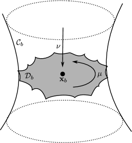
Figure 2. The Siegel cylinder $\mathcal{C}_{b}$ and the Siegel disk $\mathcal{D}_{b}$ of $H_{b}$.

The study of semi-Siegel Hénon maps had been a wide open subject until a recent work of Gaidashev, Radu, and Yampolsky (see [GaRaYam]), who proved:

Theorem 1.2 (Gaidashev-Radu-Yampolsky).

Let $\theta=\theta_{*}=(\sqrt{5}-1)/2$. Then there exists $\bar{\epsilon}>0$ such that for $b\in{\mathbb{D}}_{\bar{\epsilon}}\setminus\{0\}$, the boundary of the Siegel disk ${\mathcal{D}}_{b}$ for $H_{b}$ is a homeomorphic image of the circle. In fact, the linearizing map

$$\Psi_{b}:{\mathbb{D}}\times\{0\}\rightarrow{\mathcal{D}}_{b}$$

extends continuously and injectively (but not smoothly) to the boundary.

Recall that $H_{b}$ is an automorphism of ${\mathbb{C}}^{2}$ with constant Jacobian $b\neq 0$. Hence, $H_{b}$ does not have any definite singularities that would obstruct the smoothness of $\partial{\mathcal{D}}_{b}$ like in the one-dimensional case. Nonetheless, in the author’s joint paper with Yampolsky (see [YamY]), we proved that the Siegel boundary for a Hénon map with golden-mean rotation number is not smooth:

Theorem 1.3 (Yampolsky-Y.).

Let $\theta=\theta_{*}=(\sqrt{5}-1)/2$. Then there exists $\bar{\epsilon}>0$ such that for $b\in{\mathbb{D}}_{\bar{\epsilon}}\setminus\{0\}$, the boundary of the Siegel disk ${\mathcal{D}}_{b}$ for $H_{b}$ is not $C^{1}$-smooth.

The properties of the Siegel boundary for Hénon maps given in Theorem 1.2 and Theorem 1.3 are also true for quadratic polynomials. Our main result states that the similarity between the one and two-dimensional case does not extend to quasisymmetry:

Main Theorem (Non-Quasisymmetry).

Let $\theta=\theta_{*}=(\sqrt{5}-1)/2$. Then there exists $\bar{\epsilon}>0$ such that the set of parameter values $b$ for which the boundary of the Siegel disk ${\mathcal{D}}_{b}$ for $H_{b}$ has unbounded geometry contains a dense $G_{\delta}$ subset in the disc $\mathbb{D}_{\bar{\epsilon}}\setminus\{0\}$.

The proof of the Main Theorem follows the strategy used by de Carvalho, Lyubich and Martens in [dCLMa] to obtain the analogous result for the limit Cantor sets of Feigenbaum Hénon maps.

2. Preliminaries

In this section, we provide a brief summary of the renormalization theory of semi-Siegel Hénon maps. See [Y] for complete details.

Let $b\in{\mathbb{D}}_{\bar{\epsilon}}\setminus\{0\}$ for some $\bar{\epsilon}>0$ sufficiently small. Consider the Hénon map

$$H_{b}(x,y)=\begin{bmatrix}x^{2}+c_{b}-by\\ x\end{bmatrix}$$

that has a Siegel disc ${\mathcal{D}}_{b}\subset{\mathbb{C}}^{2}$ with rotation number $\theta_{*}=(\sqrt{5}-1)/2$.

2.1. Definition of Renormalization

Let $\hat{\Omega}_{0}$ and $\hat{\Gamma}_{0}$ be suitably chosen topological bidisks in ${\mathbb{C}}^{2}$ such that $\hat{\Omega}_{0}\cap\hat{\Gamma}_{0}\ni(0,0)$ and $\hat{\Omega}_{0}\cup\hat{\Gamma}_{0}\supset\partial{\mathcal{D}}_{b}$. The pair representation of $H_{b}$ is given by

$$\hat{\Sigma}_{0}=(\hat{A}_{0},\hat{B}_{0}):=(H_{b}|_{\hat{\Omega}_{0}},H_{b}|_{\hat{\Gamma}_{0}}).$$

Let

$$\Phi_{0}(x,y):=(\lambda_{0}x,\lambda_{0}y),$$ (2.1)

where $\lambda_{0}:=c_{b}$. Observe that

$$\Phi_{0}^{-1}\circ H_{b}\circ\Phi_{0}(0,0)=(1,0).$$

The normalized pair representation of $H_{b}$ is defined as

$$\Sigma_{0}=(A_{0},B_{0}):=(\Phi_{0}^{-1}\circ\hat{A}_{0}\circ\Phi_{0},\Phi_{0}^{-1}\circ\hat{B}_{0}\circ\Phi_{0}).$$

We may assume that for some topological discs $Z,W,V\subset{\mathbb{C}}$ containing $0$, the domains of $A_{0}$ and $B_{0}$ are given by

$$\Omega=Z\times V:=\Phi_{0}^{-1}(\hat{\Omega}_{0})\hskip 14.22636pt\text{and}\hskip 14.22636pt\Gamma=W\times V:=\Phi_{0}^{-1}(\hat{\Gamma}_{0})\hskip 14.22636pt\text{respectively.}$$

The $n$th renormalization of $H_{b}$:

$${\mathbf{R}}^{n}(H_{b}):=\Sigma_{n}=(A_{n},B_{n}),$$

where

$$A_{n}(x,y)=\begin{bmatrix}a_{n}(x,y)\\ h_{n}(x,y)\end{bmatrix}\hskip 14.22636pt\text{and}\hskip 14.22636ptB_{n}(x,y)=\begin{bmatrix}b_{n}(x,y)\\ x\end{bmatrix},$$

is the pair of rescaled iterates of $\Sigma_{0}$ defined inductively as follows. Denote

$$(a_{n})_{y}(x):=a_{n}(x,y),$$

and let

$$H_{n+1}(x,y):=\begin{bmatrix}(a_{n})_{y}^{-1}(x)\\ y\end{bmatrix}.$$

Consider the non-linear change of coordinates defined as

$$\Phi_{n+1}:=H_{n+1}\circ\Lambda_{n+1},$$

where

$$\Lambda_{n+1}(x,y)=(\lambda_{n+1}x+c_{n+1},\lambda_{n+1}y)$$ (2.2)

is an affine rescaling map to be specified later. The pair $\Sigma_{n+1}=(A_{n+1},B_{n+1})$ is defined as

$$A_{n+1}=\Phi_{n+1}^{-1}\circ B_{n}\circ A_{n}^{2}\circ\Phi_{n+1}\hskip 14.22636pt\text{and}\hskip 14.22636ptB_{n+1}=\Phi_{n+1}^{-1}\circ B_{n}\circ A_{n}\circ\Phi_{n+1}.$$

Lemma 2.1.

For $n\geq 0$, let $\Sigma_{n}=(A_{n},B_{n})$ be the $n$th renormalization of $H_{b}$. Then $A_{n}$ and $B_{n}$ are bounded analytic maps that are well-defined on $\Omega=Z\times V$ and $\Gamma=W\times V$ respectively. Moreover, the dependence of $\Sigma_{n}$ on $y$ decays super-exponentially fast. That is, we have

$$\sup_{(x,y)\in\Omega}\|\partial_{y}A_{n}(x,y)\|<C\bar{\epsilon}^{2^{n}}\hskip 14.22636pt\text{and}\hskip 14.22636pt\sup_{(x,y)\in\Gamma}\|\partial_{y}B_{n}(x,y)\|<C\bar{\epsilon}^{2^{n}}.$$

for some uniform constant $C>0$.

The one-dimensional projections of $A_{n}$, $B_{n}$ and $\Sigma_{n}$ are given by

$$\eta_{n}(x):=a_{n}(x,0)\hskip 14.22636pt,\hskip 14.22636pt\xi_{n}(x):=b_{n}(x,0)\hskip 14.22636pt\text{and}\hskip 14.22636pt\zeta_{n}:=(\eta_{n},\xi_{n})\hskip 14.22636pt\text{respectively}.$$

By Lemma 2.1, we see that $\eta_{n}$ and $\xi_{n}$ are bounded analytic functions defined on $Z$ and $W$ respectively. Moreover, the dynamics of $\Sigma_{n}$ degenerates to that of $\zeta_{n}$ super-exponentially fast. It is shown in [Y] that $\eta_{n}$ and $\xi_{n}$ each have a unique simple critical point which are $C\bar{\epsilon}^{2^{n}}$-close to each other. We choose the normalizing constants $\lambda_{n}$ and $c_{n}$ in (2.2) so that

$$\xi_{n}(0)=1\hskip 14.22636pt\text{and}\hskip 14.22636pt\xi_{n}^{\prime}(0)=0.$$

2.2. Renormalization Convergence

Let $\zeta_{*}=(\eta_{*},\xi_{*})$ be the fixed point of the one-dimensional renormalization operator ${\mathcal{R}}$ given in [GaYam]. In particular, we have

$$\lambda_{*}^{-1}\eta_{*}\circ\xi_{*}\circ\eta_{*}(\lambda_{*}x)=\eta_{*}(x)\hskip 14.22636pt\text{and}\hskip 14.22636pt\lambda_{*}^{-1}\eta_{*}\circ\xi_{*}(\lambda_{*}x)=\xi_{*}(x),$$ (2.3)

where

$$\lambda_{*}:=\eta_{*}\circ\xi_{*}(0)\in{\mathbb{D}}$$

is the universal scaling factor.

Convergence under renormalization for semi-Siegel Hénon maps was first obtained in [GaYam]. For the renormalization operator ${\mathbf{R}}$ defined above, the proof of convergence is given in [Y].

Theorem 2.2.

As $n\to\infty$, we have the following convergences (each of which occurs at a geometric rate):

1. $\zeta_{n}=(\eta_{n},\xi_{n})\to\zeta_{*}=(\eta_{*},\xi_{*})$;

2. $\lambda_{n}\to\lambda_{*}$; and

3. $\Phi_{n}\to\Phi_{*}$, where

   $$\Phi_{*}(x,y)=\begin{bmatrix}\phi_{*}(x)\\ \lambda_{*}y\end{bmatrix}:=\begin{bmatrix}\eta_{*}^{-1}(\lambda_{*}x)\\ \lambda_{*}y\end{bmatrix}.$$

2.3. Renormalization Limit Set

Define the $n$th microscope map of depth $k$ by

$$\Phi_{n}^{n+k}:=\Phi_{n+1}\circ\Phi_{n+2}\circ\ldots{}\circ\Phi_{n+k}.$$

Let

$$\Omega_{n}^{n+k}:=\Phi_{n}^{n+k}(\Omega)\hskip 14.22636pt\text{and}\hskip 14.22636pt\Gamma_{n}^{n+k}:=\Phi_{n}^{n+k}(\Gamma).$$

Observe that $\{\Omega_{n}^{n+k}\cup\Gamma_{n}^{n+k}\}_{k=0}^{\infty}$ is a nested sequence of open sets. See Figure 3

Proposition 2.3.

Let $\lambda_{*}\in{\mathbb{D}}$ be the universal scaling factor. Then for all $0\leq n,k$, we have

$$\text{\emph{diam}}(\Omega_{n}^{n+k}\cup\Gamma_{n}^{n+k})=O(|\lambda_{*}|^{k}).$$

Consequently, there exists a point $(\kappa_{n},0)\in\Omega$, called the $n$th cap, such that

$$\bigcap_{k=0}^{\infty}\Omega_{n}^{n+k}\cup\Gamma_{n}^{n+k}=(\kappa_{n},0).$$

Moreover, $\kappa_{n}$ converges to $1$ geometrically fast as $n\to\infty$.

Remark 2.4.

The cap is a dynamically defined point with the same combinatorial address as the critical value $\xi_{*}(0)=1$. In [dCLMa], the analog of the critical value is referred to as the tip.

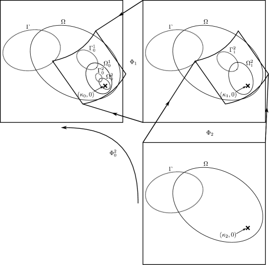
Figure 3. The renormalization microscope map $\Phi_{0}^{2}$ obtained by composing the non-linear changes of coordinates $\Phi_{1}$ and $\Phi_{2}$. We have $\Omega_{0}^{1}=\Phi_{1}(\Omega)$, $\Gamma_{0}^{1}=\Phi_{1}(\Gamma)$, $\Omega_{0}^{2}=\Phi_{0}^{2}(\Omega)$, $\Gamma_{0}^{2}=\Phi_{0}^{2}(\Gamma)$, and $(\kappa_{0},0)=\Phi_{1}((\kappa_{1},0))=\Phi_{0}^{2}((\kappa_{2},0))$.

Denote

$$\hat{\Omega}_{n}:=\Phi_{0}\circ\Phi_{0}^{n}(\Omega)\hskip 14.22636pt\text{and}\hskip 14.22636pt\hat{\Gamma}_{n}:=\Phi_{0}\circ\Phi_{0}^{n}(\Gamma),$$

where $\Phi_{0}$ is given in (2.1).

Lemma 2.5.

Let $\{q_{n}\}_{n=0}^{\infty}$ be the Fibonacci sequence. Define

$$\hat{A}_{n}:=H_{b}^{q_{2n+1}}|_{\hat{\Omega}_{n}}\hskip 14.22636pt\text{and}\hskip 14.22636pt\hat{B}_{n}:=H_{b}^{q_{2n}}|_{\hat{\Gamma}_{n}}.$$

Then the $n$th renormalization $\Sigma_{n}=(A_{n},B_{n})$ is given by

$$A_{n}=(\Phi_{0}^{n})^{-1}\circ\Phi_{0}^{-1}\circ\hat{A}_{n}\circ\Phi_{0}\circ\Phi_{0}^{n},\hskip 14.22636pt\text{and}\hskip 14.22636ptB_{n}=(\Phi_{0}^{n})^{-1}\circ\Phi_{0}^{-1}\circ\hat{B}_{n}\circ\Phi_{0}\circ\Phi_{0}^{n}.$$

In [GaRaYam], Gaidashev, Radu and Yampolsky showed that the renormalization limit set for a semi-Siegel Hénon map coincides with its Siegel boundary:

Theorem 2.6.

For $n\in\mathbb{N}$, let

$$X_{n}:=\bigcup_{i=0}^{q_{2n+1}-1}H_{b}^{i}(\hat{\Omega}_{n})\hskip 14.22636pt\text{and}\hskip 14.22636ptY_{n}:=\bigcup_{i=0}^{q_{2n}-1}H_{b}^{i}(\hat{\Gamma}_{n}).$$

Then the Siegel boundary for $H_{b}$ is given by

$$\partial{\mathcal{D}}_{b}:=\bigcap_{n=1}^{\infty}X_{n}\cup Y_{n}.$$

3. Universality

The proof of the main theorem involves giving precise estimates for various geometric quantities that arise when analyzing the dynamics of the semi-Siegel Hénon map $H_{b}$ near its Siegel boundary $\partial{\mathcal{D}}_{b}$. In order to do this, we first need an explicit description for the $n$th renormalization $\Sigma_{n}=(A_{n},B_{n})$ of $H_{b}$. In [Y], the author showed that $\Sigma_{n}$ has a universal first-order approximation in terms of its Jacobian. In this section, we strengthen this result to better suit our application.

As before, we write

$$A_{n}(x,y)=\begin{bmatrix}a_{n}(x,y)\\ h_{n}(x,y)\end{bmatrix}\hskip 14.22636pt\text{and}\hskip 14.22636ptB_{n}(x,y)=\begin{bmatrix}b_{n}(x,y)\\ x\end{bmatrix}.$$

Recall that $A_{n}$ and $B_{n}$ represent the $q_{2n+1}$th and $q_{2n}$th iterate of $H_{b}$ respectively. Accordingly, we expect the Jacobian of $A_{n}$ and $B_{n}$ to be on the order of

$$b^{q_{2n+1}}=\operatorname{Jac}H_{b}^{q_{2n+1}}\hskip 14.22636pt\text{and}\hskip 14.22636ptb^{q_{2n}}=\operatorname{Jac}H_{b}^{q_{2n}}\hskip 14.22636pt\text{respectively}.$$

The following theorem is a simplification of Theorem 7.3 in [Y] in the case when the map being renormalized has constant Jacobian. In the general, non-constant Jacobian case, the dependence of $b_{n}$ on $y$ has a factor of $e^{r_{n}}$ for some uniformly bounded sequence $\{r_{n}\}_{n=0}^{\infty}\subset{\mathbb{C}}$. This is to account for small fluctuations caused by variation in the Jacobian along the renormalization limit set.

Theorem 3.1.

For $n\geq 0$, we have

$$B_{n}(x,y)=\begin{bmatrix}\xi_{n}(x)-b^{q_{2n}}\,\beta(x)\,y\,(1+O(\rho^{n}))\\ x\end{bmatrix},$$

where $0<\rho<1$ is a uniform constant; and $\beta(x)$ is a universal function that is uniformly bounded away from $0$ and $\infty$, and has a uniformly bounded derivative and distortion.

Observe that

$$\operatorname{Jac}B_{n}(x,y) =\begin{vmatrix}\xi_{n}^{\prime}(x)-b^{q_{2n}}\,\beta^{\prime}(x)\,y&-b^{q_{2n}}\,\beta(x)\\ 1&0\end{vmatrix}+\text{(higher order terms)}$$

$$=-b^{q_{2n}}\,\beta(x)+\text{(higher order terms)}$$ (3.1)

as we expected.

Next, we give a first-order approximation of $A_{n}$. In [Y], this is only done for the first coordinate $a_{n}$ (see Corollary 7.4).

Theorem 3.2.

For $n\geq 0$, we have

$$A_{n}(x,y)=\begin{bmatrix}\eta_{n}(x)-b^{q_{2n}}\,\alpha(x)\,y\,(1+O(\rho^{n}))\\ \lambda_{n}^{-1}\check{\eta}_{n-1}(\lambda_{n}x)-b^{q_{2n}}\,\check{\alpha}(x)\,y\,(1+O(\rho^{n}))\end{bmatrix},$$

where $0<\rho<1$ is a uniform constant; and

$$\check{\eta}_{k}(x)=\eta_{k}(x)+O(|b|^{q_{2k}})\hskip 8.53581pt,\hskip 8.53581pt\alpha(x):=\frac{\eta_{*}^{\prime}(x)}{\xi_{*}^{\prime}(x)}\beta(x)\hskip 8.53581pt\text{and}\hskip 8.53581pt\check{\alpha}(x):=\frac{\eta_{*}^{\prime}(\lambda_{*}x)}{\eta_{*}^{\prime}(x)}\alpha(x).$$

Proof.

Recall that

$$A_{n+1}:=\Lambda_{n+1}^{-1}\circ H_{n+1}^{-1}\circ B_{n}\circ A_{n}^{2}\circ H_{n+1}\circ\Lambda_{n+1}.$$ (3.2)

Denote

$$(\tilde{x},\tilde{y}):=\Lambda_{n+1}(x,y)=(\lambda_{n+1}x+c_{n+1},\lambda_{n+1}y).$$

It is not difficult to show, using Theorem 3.1, that $c_{n+1}=O(|b|^{q_{2n}})$. Moreover, we have

$$A_{n}\circ H_{n+1}(x,y)=\begin{bmatrix}x\\ \tilde{h}_{n}(x,y)\end{bmatrix},$$

where

$$\tilde{h}_{n}(x,y):=h_{n}((a_{n})_{y}^{-1}(x),y).$$

Hence,

$$h_{n+1}(x,y)=\lambda_{n+1}^{-1}a_{n}(\tilde{x},\tilde{h}_{n}(\tilde{x},\tilde{y}))=\lambda_{n+1}^{-1}\eta_{n}(\lambda_{n+1}x)+O(|b|^{q_{2n}}).$$ (3.3)

Since $A_{n}$ and $B_{n}$ commute, we may rearrange the terms in (3.2) to obtain

$$A_{n+1}=\Lambda_{n+1}^{-1}\circ H_{n+1}^{-1}\circ A_{n}\circ H_{n+1}\circ\Lambda_{n+1}\circ B_{n+1}.$$

Denote

$$\tilde{\xi}_{n+1}(x):=\lambda_{n+1}\xi_{n+1}(x)+c_{n+1}$$

and

$$\tilde{b}_{n+1}(x,y) :=\lambda_{n+1}b_{n+1}(x,y)+c_{n+1}$$

$$=\tilde{\xi}_{n+1}(x)-\lambda_{n+1}b^{q_{2(n+1)}}\beta(x)y(1+O(\rho^{n+1})).$$

Then

$$H_{n+1}\circ\Lambda_{n+1}\circ B_{n+1}(x,y)=\begin{bmatrix}(a_{n})_{\tilde{x}}^{-1}(\tilde{b}_{n+1}(x,y))\\ \tilde{x}\end{bmatrix}.$$

Neglecting higher order terms, $(a_{n})_{\tilde{x}}^{-1}(\tilde{b}_{n+1}(x,y))$ has the same $y$-dependence as

$$\eta_{n}^{-1}(\tilde{b}_{n+1}(x,y))\approx\eta_{n}^{-1}(\tilde{\xi}_{n+1}(x))-(\eta_{n}^{-1})^{\prime}(\tilde{\xi}_{n+1}(x))\lambda_{n+1}b^{q_{2(n+1)}}\beta(x)y$$

Let

$$\check{x}:=\lambda_{n}\eta_{n}^{-1}(\tilde{\xi}_{n+1}(x)).$$

From (3.3), and again neglecting higher order terms, we see that the second coordinate $h_{n}\big{(}(a_{n})_{\tilde{x}}^{-1}(\tilde{b}_{n+1}(x,y)),\tilde{x}\big{)}$ has the same $y$-dependence as

$$\lambda_{n}^{-1}\eta_{n-1}\big{(}\lambda_{n}\eta_{n}^{-1}(\tilde{b}_{n+1}(x,y))\big{)}\approx\lambda_{n}^{-1}\eta_{n-1}(\check{x})-\eta_{n-1}^{\prime}(\check{x})(\eta_{n}^{-1})^{\prime}(\tilde{\xi}_{n+1}(x))\lambda_{n+1}b^{q_{2(n+1)}}\beta(x)y.$$

Lastly, we compute

$$\lim_{n\to\infty}\eta_{n-1}^{\prime}(\check{x})(\eta_{n}^{-1})^{\prime}(\tilde{\xi}_{n+1}(x)) =\eta_{*}^{\prime}\big{(}\lambda_{*}\eta_{*}^{-1}(\lambda_{*}\xi_{*}(x))\big{)}(\eta_{*}^{-1})^{\prime}(\lambda_{*}\xi_{*}(x))$$

$$=\eta_{*}^{\prime}\big{(}\eta_{*}\circ\xi_{*}(\lambda_{*}^{2}x))\big{)}(\eta_{*}^{-1})^{\prime}(\eta_{*}\circ\xi_{*}(\lambda_{*}x))$$

$$=\frac{\eta_{*}^{\prime}\big{(}\eta_{*}\circ\xi_{*}(\lambda_{*}^{2}x)\big{)}}{\eta_{*}^{\prime}(\xi_{*}(\lambda_{*}x))}$$

$$=\frac{\eta_{*}^{\prime}(\lambda_{*}x)}{\xi_{*}^{\prime}(\lambda_{*}x)}\cdot\frac{\xi_{*}^{\prime}(\lambda_{*}x)}{\xi_{*}^{\prime}(x)}$$

$$=\frac{\eta_{*}^{\prime}(\lambda_{*}x)}{\xi_{*}^{\prime}(x)},$$

where in the second equality, we used (2.3) and in the third equality, we used the derivative of (2.3). The result follows. ∎

Observe:

$$\operatorname{Jac}A_{n}(x,y) =\begin{vmatrix}\eta_{n}^{\prime}(x)-b^{q_{2n}}\,\alpha^{\prime}(x)\,y&-b^{q_{2n}}\,\alpha(x)\\ \check{\eta}_{n-1}^{\prime}(\lambda_{n}x)-b^{q_{2n}}\,\check{\alpha}^{\prime}(x)\,y&-b^{q_{2n}}\,\check{\alpha}(x)\end{vmatrix}+\text{(higher order terms)}$$

$$=\big{(}-\eta_{n}^{\prime}(x)\,\check{\alpha}(x)+\check{\eta}_{n-1}^{\prime}(\lambda_{n}x)\,\alpha(x)\big{)}b^{q_{2n}}+\text{(higher order terms)}$$

$$=\big{(}-\eta_{*}^{\prime}(x)\,\check{\alpha}(x)+\eta_{*}^{\prime}(\lambda_{*}x)\,\alpha(x)\big{)}b^{q_{2n}}+\text{(higher order terms)}$$

$$=\text{(higher order terms)}.$$

Hence, we see that the first-order approximation of $A_{n}$ is not precise enough to “see” the Jacobian of $A_{n}$, which we expect to be of higher order ($b^{q_{2n+1}}$ rather than $b^{q_{2n}}$). Fortunately, the approximation can be made much more precise by considering $A_{n}\circ\Phi_{n+1}$ instead of $A_{n}$.

Theorem 3.3.

For $n\geq 0$, we have

$$A_{n}\circ\Phi_{n+1}(x,y)=\begin{bmatrix}\lambda_{n+1}x+c_{n+1}\\ \check{\xi}_{n}^{-1}(\lambda_{n+1}x)-b^{q_{2n+1}}\,\chi(x)\,\lambda_{n+1}\,y(1+O(\rho^{n}))\end{bmatrix},$$

where $0<\rho<1$ is a uniform constant; and

$$\check{\xi}_{n}(x)=\xi_{n}(x)+O(|b|^{q_{2(n-1)}})\hskip 8.53581pt\text{and}\hskip 8.53581pt\chi(x):=\frac{\xi_{*}^{\prime}(\lambda_{*}x)}{\xi_{*}^{\prime}(x)}\frac{\beta(x)}{\beta(\lambda_{*}x)}=\frac{\eta_{*}^{\prime}(\lambda_{*}x)}{\eta_{*}^{\prime}(x)}\frac{\alpha(x)}{\alpha(\lambda_{*}x)}.$$

Proof.

Write

$$A_{n}\circ H_{n+1}(x,y)=\begin{bmatrix}x\\ \tilde{h}_{n}(x,y)\end{bmatrix},$$

where

$$\tilde{h}_{n}(x,y):=h_{n}((a_{n})_{y}^{-1}(x),y).$$

By Theorem 3.2, we have

$$\tilde{h}_{n}(x,y)=\lambda_{n}^{-1}\eta_{n-1}(\lambda_{n}\eta_{n}^{-1}(x))+O(|b|^{q_{2(n-1)}}).$$ (3.4)

By definition, $\eta_{n}(x)=a_{n}(x,0)$, where $a_{n}$ is the first coordinate of $A_{n}$. Since $A_{n-1}$ and $B_{n-1}$ commute, we have

$$A_{n}:=\Phi_{n}^{-1}\circ B_{n-1}\circ A_{n-1}^{2}\circ\Phi_{n}=B_{n}\circ\Phi_{n}^{-1}\circ A_{n-1}\circ\Phi_{n}.$$

Thus,

$$\eta_{n}=\xi_{n}(\lambda_{n}^{-1}\eta_{n-1}(\lambda_{n}x))+O(|b|^{q_{2(n-1)}}).$$ (3.5)

Taking the inverse of (3.5) and plugging into (3.4), we obtain

$$\lambda_{n}^{-1}\eta_{n-1}(\lambda_{n}\eta_{n}^{-1}(x))=\xi_{n}^{-1}(x)+O(|b|^{q_{2(n-1)}}).$$

To derive the first-order approximation of the $y$-dependence of $A_{n}\circ\Phi_{n+1}$, consider

$$B_{n+1}=\Phi_{n+1}^{-1}\circ B_{n}\circ A_{n}\circ\Phi_{n+1}.$$

Taking the Jacobian, we obtain

$$\operatorname{Jac}_{{\mathbf{x}}_{0}}(B_{n+1})=\operatorname{Jac}_{{\mathbf{x}}_{2}}(\Phi_{n+1}^{-1})\cdot\operatorname{Jac}_{{\mathbf{x}}_{1}}(B_{n})\cdot\operatorname{Jac}_{{\mathbf{x}}_{0}}(A_{n}\circ\Phi_{n+1}),$$ (3.6)

where

$${\mathbf{x}}_{0}:=(x,y)\hskip 14.22636pt,\hskip 14.22636pt{\mathbf{x}}_{1}=(x_{1},y_{1}):=A_{n}\circ\Phi_{n+1}({\mathbf{x}}_{0})\hskip 14.22636pt\text{and}\hskip 14.22636pt{\mathbf{x}}_{2}=(x_{2},y_{2}):=B_{n}({\mathbf{x}}_{1}).$$

Neglecting higher order terms, we have

$$x_{1}\approx\lambda_{n+1}x\hskip 14.22636pt\text{and}\hskip 14.22636ptx_{2}\approx\xi_{n}(\lambda_{n+1}x).$$

By (3.1), it follows that

$$\operatorname{Jac}_{{\mathbf{x}}_{0}}(B_{n+1})\approx b^{q_{2n+2}}\beta(x)\hskip 14.22636pt\text{and}\hskip 14.22636pt\operatorname{Jac}_{{\mathbf{x}}_{1}}(B_{n})\approx b^{q_{2n}}\beta(\lambda_{n+1}x).$$ (3.7)

Observe:

$$\operatorname{Jac}_{{\mathbf{x}}_{2}}\Phi_{n+1}^{-1} =\lambda_{n+1}^{-2}\begin{vmatrix}\partial_{x}a_{n}({\mathbf{x}}_{2})&\partial_{y}a_{n}({\mathbf{x}}_{2})\\ 0&1\end{vmatrix}$$

$$\approx\lambda_{n+1}^{-2}\eta_{n}^{\prime}(\xi_{n}(\lambda_{n+1}x)).$$ (3.8)

Plugging in (3.7) and (3.8) into (3.6), we obtain

$$\operatorname{Jac}_{{\mathbf{x}}_{0}}(A_{n}\circ\Phi_{n+1})\approx b^{q_{2n+1}}\lambda_{n+1}^{2}\frac{\beta(x)}{\beta(\lambda_{n+1}x)}\eta_{n}^{\prime}(\xi_{n}(\lambda_{n+1}x)).$$ (3.9)

Lastly, write:

$$A_{n}\circ\Phi_{n+1}(x,y)=\begin{bmatrix}\lambda_{n+1}x+c_{n+1}\\ \tilde{h}_{n}(x,0)+E_{n}(x,y)\end{bmatrix},$$

where $E_{n}(x,y)$ is undetermined. Since

$$\operatorname{Jac}_{(x,y)}(A_{n}\circ\Phi_{n+1})=\lambda_{n+1}\partial_{y}E_{n}(x,y),$$

plugging in (3.9) and integrating both sides, we obtain the desired formula. ∎

Recall that the $n$th cap $(\kappa_{n},0)\in\Omega$ is a dynamically defined point in the renormalization limit set for $\Sigma_{n}$. It is not difficult to see that we have

$$\Phi_{n}((\kappa_{n},0))=(\kappa_{n-1},0)\hskip 14.22636pt\text{and}\hskip 14.22636pt\Phi_{n}^{n+k}((\kappa_{n+k},0))=(\kappa_{n},0).$$

Denote

$$D_{n}:=D_{(\kappa_{n},0)}\Phi_{n}\hskip 14.22636pt\text{and}\hskip 14.22636ptD_{n}^{n+k}:=D_{(\kappa_{n+k},0)}\Phi_{n}^{n+k}.$$

Observe

$$D_{n}^{n+k}=D_{n+1}\cdot D_{n+2}\cdot\ldots{}\cdot D_{n+k}.$$

The following estimates on the derivative the microscope maps at the cap is a corollary of Theorem 3.2. The statement is more precise than the one given in [Y], but it follows from the same proof.

Theorem 3.4.

Write

$$D_{n}=\begin{bmatrix}1&t_{n}b^{q_{2(n-1)}}\\ 0&1\end{bmatrix}\begin{bmatrix}u_{n}&0\\ 0&\lambda_{n}\end{bmatrix}.$$

Then there exist a uniform positive constant $\rho<1$ such that the following estimates hold for all $n\geq 1$:

1. $u_{n}=\lambda_{*}^{2}(1+O(\rho^{n}))$,

2. $\lambda_{n}=\lambda_{*}(1+O(\rho^{n}))$, and

3. $t_{n}=\lambda_{*}\alpha(1)(1+O(\rho^{n}))$.

Consequently, for $0\leq n,k$, we have

$$D_{n}^{n+k}=\begin{bmatrix}1&t_{n}^{n+k}b^{q_{2n}}\\ 0&1\end{bmatrix}\begin{bmatrix}u_{n}^{n+k}&0\\ 0&\lambda_{n}^{n+k}\end{bmatrix},$$

where

1. $u_{n}^{n+k}:=u_{n+1}\cdot u_{n+1}\cdot\ldots\cdot u_{n+k}=\lambda_{*}^{2k}(1+O(\rho^{n}))$,

2. $\lambda_{n}^{n+k}:=\lambda_{n+1}\cdot\lambda_{n+2}\cdot\ldots\cdot\lambda_{n+k}=\lambda_{*}^{k}(1+O(\rho^{n}))$, and

3. $t_{n}^{n+k}=t_{n+1}(1+O(|b|^{q_{2n+1}}))$.

4. Proof of Non-Quasisymmetry

Definition 4.1.

Let $\gamma$ be a continuous arc or a simple closed curve. For $x,y\in\gamma$, let $[x,y]_{\gamma}$ denote the smallest subarc of $\gamma$ with endpoints at $x$ and $y$. We say that $\gamma$ is $K$-quasisymmetric for some $K>0$ if

$$\operatorname{diam}([x,y]_{\gamma})<K\operatorname{dist}(x,y)\hskip 14.22636pt\text{for all}\hskip 14.22636ptx,y\in\gamma.$$

If $\gamma$ is not $K$-quasisymmetric for all $K>0$, then we say that $\gamma$ has unbounded geometry.

Proof of the Main Theorem.

Let $n,k\in{\mathbb{N}}$ be sufficiently large. To prove the desired result, we analyze the geometry of the Siegel boundary $\partial{\mathcal{D}}_{b}$ in three different scales: that of $\Sigma_{n+k}$, $\Sigma_{n}$ and $\Sigma_{0}$.

We start in the scale of $\Sigma_{n+k}$. Consider the dynamically defined points

$${\mathbf{q}}_{n+k}:=(\kappa_{n+k},0)\hskip 14.22636pt\text{and}\hskip 14.22636pt{\mathbf{p}}_{n+k}:=A_{n+k}({\mathbf{q}}_{n+k}).$$

Next, in the scale of $\Sigma_{n}=(A_{n},B_{n})$, consider

$${\mathbf{q}}_{n}^{n+k}:=A_{n}\circ\Phi_{n}^{n+k}({\mathbf{q}}_{n+k})=A_{n}((\kappa_{n},0))\hskip 14.22636pt\text{and}\hskip 14.22636pt{\mathbf{p}}_{n}^{n+k}:=A_{n}\circ\Phi_{n}^{n+k}({\mathbf{p}}_{n+k}).$$

Lastly, in the scale of $\Sigma_{0}$, consider

$${\mathbf{q}}_{0}^{n+k}:=\Phi_{0}^{n}({\mathbf{q}}_{n}^{n+k})\hskip 14.22636pt\text{and}\hskip 14.22636pt{\mathbf{p}}_{0}^{n+k}:=\Phi_{0}^{n}({\mathbf{p}}_{n}^{n+k}).$$

See Figure 4.

It is easy to see that

$${\mathbf{q}}_{0}^{n+k}=H_{b}^{i}((\kappa_{0},0))\in\partial{\mathcal{D}}_{b}\hskip 14.22636pt\text{and}\hskip 14.22636pt{\mathbf{p}}_{0}^{n+k}=H_{b}^{j}((\kappa_{0},0))\in\partial{\mathcal{D}}_{b}.$$

for some $i,j\in{\mathbb{N}}$. Denote the $x$- and $y$-coordinate of ${\mathbf{q}}_{n+k}-{\mathbf{p}}_{n+k}$ by $\Delta_{n+k}x$ and $\Delta_{n+k}y$ respectively. The $x$- and $y$-coordinates of ${\mathbf{q}}_{n}^{n+k}-{\mathbf{q}}_{n}^{n+k}$ and ${\mathbf{q}}_{0}^{n+k}-{\mathbf{p}}_{0}^{n+k}$ are denoted similarly, but with $\Delta_{n}^{n+k}$ and $\Delta_{0}^{n+k}$ respectively instead of $\Delta_{n+k}$.

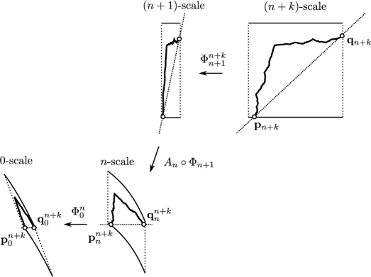
Figure 4. Exploiting universality to create a cusp in the Siegel boundary $\partial{\mathcal{D}}_{b}$.

First, note that $\Delta_{n+k}\,x$ and $\Delta_{n+k}\,y$ converge to some uniform limits $\Delta_{*}\,x$ and $\Delta_{*}\,y$ respectively as $k\to\infty$. By Theorem 3.3 and 3.4, we have:

$$\Delta_{n}^{n+k}\,x=\lambda_{*}^{2k-1}\Delta_{*}\,x(1+O(\rho^{n}))$$ (4.1)

and

$$\Delta_{n}^{n+k}\,y=\lambda_{*}^{k-1}(\lambda_{*}^{k}C_{1}-b^{q_{2n+1}}C_{2})(1+O(\rho^{n})),$$ (4.2)

where

$$C_{1}:=(\xi_{*}^{-1})^{\prime}(\lambda_{*})\Delta_{*}\,x\hskip 14.22636pt\text{and}\hskip 14.22636ptC_{2}:=\lambda_{*}\chi(1)\Delta_{*}\,y$$

are uniform constants.

The values of $b$ that solve

$$b^{q_{2n+1}}=\frac{C_{1}}{C_{2}}\lambda_{*}^{k}$$

as $k$ and $n$ run through $\mathbb{N}$ is dense in $\mathbb{D}_{\bar{\epsilon}}$. Let $\mathbb{B}_{m}\subset{\mathbb{D}}_{\bar{\epsilon}}$ be the set of parameter values such that for some $n\geq m$ and $k\in\mathbb{N}$, we have

$$|b|^{q_{2n+1}}\asymp|\lambda_{*}|^{k}$$

and

$$\Delta_{n}^{n+k}\,y=O(|\lambda_{*}|^{n+2k}).$$ (4.3)

Then $\mathbb{B}_{m}$ is a dense open set of $\mathbb{D}_{\bar{\epsilon}}$. Hence, the intersection

$$\mathbb{B}_{\infty}:=\bigcap_{m=N}^{\infty}\mathbb{B}_{m}$$

is a $G_{\delta}$-subset of $\mathbb{D}_{\bar{\epsilon}}$, consisting of parameters $b$ for which (4.3) holds for infinitely many $n\in{\mathbb{N}}$.

Assume that $b\in\mathbb{B}_{\infty}$ and that (4.3) holds for $n$ and $k$. By Theorem 3.4, we have:

$$\Delta_{0}^{n+k}\,x\asymp\lambda_{*}^{2n}\Delta_{n}^{n+k}\,x\asymp\lambda_{*}^{2n+2k-1}$$

and

$$\Delta_{0}^{n+k}\,y\asymp\lambda_{*}^{n}\Delta_{n}^{n+k}\,y=O(|\lambda_{*}|^{2n+2k})$$

Hence:

$$\operatorname{dist}({\mathbf{q}}_{0}^{n+k},{\mathbf{p}}_{0}^{n+k})=O(|\lambda_{*}|^{2n+2k}).$$ (4.4)

We now estimate the diameter of the subarc $[{\mathbf{q}}_{0}^{n+k},{\mathbf{p}}_{0}^{n+k}]_{\partial{\mathcal{D}}_{b}}$. Consider the points

$$\check{{\mathbf{q}}}_{n+k}:=\Phi_{n+k+1}\circ A_{n+k+1}((\kappa_{n+k+1},0))\hskip 14.22636pt,\hskip 14.22636pt\check{{\mathbf{q}}}_{n}^{n+k}:=A_{n}\circ\Phi_{n}^{n+k}(\check{{\mathbf{q}}}_{n+k})$$

$$\hskip 14.22636pt\text{and}\hskip 14.22636pt\check{{\mathbf{q}}}_{0}^{n+k}:=\Phi_{0}^{n}(\check{{\mathbf{q}}}_{n}^{n+k}).$$

It is easy to see that $\check{{\mathbf{q}}}_{0}^{n+k}\in[{\mathbf{q}}_{0}^{n+k},{\mathbf{p}}_{0}^{n+k}]_{\partial{\mathcal{D}}_{b}}$. Denote the $x$- and $y$-coordinate of $\check{{\mathbf{q}}}_{n+k}-{\mathbf{q}}_{n+k}$ by $\check{\Delta}_{n+k}\,x$ and $\check{\Delta}_{n+k}\,y$ respectively. The $x$- and $y$-coordinates of $\check{{\mathbf{q}}}_{n}^{n+k}-{\mathbf{q}}_{n}^{n+k}$ and $\check{{\mathbf{q}}}_{0}^{n+k}-{\mathbf{q}}_{0}^{n+k}$ are denoted similarly, but with $\check{\Delta}_{n}^{n+k}$ and $\check{\Delta}_{0}^{n+k}$ respectively instead of $\Delta_{n+k}$.

Note that $\check{\Delta}_{n+k}\,x$ and $\check{\Delta}_{n+k}\,y$ converge to $\lambda_{*}^{2}\Delta_{*}\,x$ and $\lambda_{*}\Delta_{*}\,y$ respectively as $k\to\infty$. By similar considerations as for (4.1) and (4.2), we obtain

$$\check{\Delta}_{n}^{n+k}\,x=\lambda_{*}^{2k+1}\Delta_{*}\,x(1+O(\rho^{n}))$$

and

$$\check{\Delta}_{n}^{n+k}\,y =\lambda_{*}^{k}(\lambda_{*}^{k+1}C_{1}-b^{q_{2n+1}}C_{2})(1+O(\rho^{n}))$$

$$=\lambda_{*}^{2k}C_{1}\left(\lambda_{*}-\frac{b^{q_{2n+1}}C_{2}}{\lambda_{*}^{k}C_{1}}\right)(1+O(\rho^{n})).$$

Since $\lambda_{*}<1$, it follows from (4.3) that $\check{\Delta}_{n}^{n+k}\,y\asymp\lambda_{*}^{2k}$. Hence,

$$\check{\Delta}_{0}^{n+k}\,y\asymp\lambda_{*}^{n}\check{\Delta}_{0}^{n+k}\asymp\lambda_{*}^{n+2k}.$$

Therefore,

$$\frac{\operatorname{diam}([{\mathbf{q}}_{0}^{n+k},{\mathbf{p}}_{0}^{n+k}]_{\partial{\mathcal{D}}_{b}})}{\operatorname{dist}({\mathbf{q}}_{0}^{n+k},{\mathbf{p}}_{0}^{n+k})}\geq\frac{\operatorname{dist}(\check{{\mathbf{q}}}_{0}^{n+k},{\mathbf{q}}_{0}^{n+k})}{\operatorname{dist}({\mathbf{q}}_{0}^{n+k},{\mathbf{p}}_{0}^{n+k})}\asymp\lambda_{*}^{-n}\to\infty\hskip 14.22636pt\text{as}\hskip 14.22636ptn\to\infty.$$

The result follows. ∎