A Computational Model for Bacterial Run-and-Tumble Motion

Abstract

In our article we present a computational model for the simulation of self-propelled anisotropic bacteria. To this end we use a self-propelled particle model and augment it with a statistical algorithm for the run-and-tumble motion. We derive an equation for the distribution of reorientations of the bacteria that we use to analyze the statistics of the random walk and that allows us to tune the behavior of our model to the characteristics of an E.coli bacterium. We validate our implementation in terms of a single swimmer and demonstrate that our model is capable of reproducing E. coli’s run-and-tumble motion with excellent accuracy.

I Introduction

Living organisms like bacteria have developed several strategies to enable their survival. One of the strategies that are particular to flagellated bacteria is the so-called run-and-tumble (RT) motion, which helps them to explore the surroundings and find food. Such run-and-tumble bacteria, e.g., E. coli, swim straight for a certain amount of time and rather abruptly change the swimming directions Berg and Brown (1972); Berg (1993). However, in models for bacteria this behavior is often neglected or coarse-grained out by using a stochastic description fixing only the diffusion coefficients, which results in ignoring the precise information contained in the spatial trajectories of RT bacteria. Another downside of approaches such as active Brownian dynamics is that they do not include hydrodynamical interactions. Although a stochastic description is one of the most powerful tools to study and understand a bacterial system Ebeling, Schweitzer, and Tilch (1999); Elgeti and Gompper (2013, 2015); Ezhilan, Alonso-Matilla, and Saintillan (2015); Cates and Tailleur (2013); Cates (2012), these downsides can miss important physical interactions when studying the collective behavior of bacteria in complex environments.

There have been studies on individual bacteria, mainly on the hydrodynamic interactions of a bacterium with its surroundings Lighthill (1952); Blake (1971); Winkler (2016); Lauga (2011); Zöttl and Stark (2016). Since the flow fields induced by bacteria decay rather slowly ($\sim r^{-2}$) Lighthill (1952); Blake (1971); Winkler (2016), the inclusion of hydrodynamical interactions seems to be a necessary ingredient in modeling bacterial motion. In this article we therefore present a novel numerically efficient implementation of an elongated self-propelled bacteria model that performs a RT motion and is able to hydrodynamically interact with other bacteria and complex obstacles or interfaces.

The article is organized as follows. In Section II, we review experimental discoveries and theoretical studies of RT motion Berg and Brown (1972); Berg (1993); Saragosti, Silberzan, and Buguin (2012); Lovely and Dahlquist (1975). Then, we derive a formula that can be used to analyze the trajectory of a RT motion. In Section III we introduce a molecular dynamics (MD) force-free swimmer model that is implemented by coupling the bacterium to a lattice-Boltzmann algorithm (LB-MD) Dünweg and Ladd (2009); Ahlrichs and Dünweg (1999); Krüger et al. (2017); Succi (2001); de Graaf et al. (2016a, b). Further, we describe our method that is running on top of this swimmer model that steers the RT motion. This will enable us to efficiently study a system with multiple interacting run-and-tumble bacteria. The algorithm itself is, however, not bounded to a certain simulation method, so it can run on top of any conventional numerical scheme. In Section IV, we present and analyze the trajectory results for a single swimmer. There, we fix the relevant RT algorithmic parameters of the swimmer to match the characteristics of E. coli bacteria and demonstrate that our model can reproduce the experimentally observed swimming trajectories.

II Statistical theory of the run-and-tumble motion

In the following, we build a mathematical model for bacterial RT motion by means of statistical theory. A RT motion is characterized by the following three distributions: the durations of runs, tumbles and reorientations.

Throughout the statistical derivation we assume that

• the swimmer does not change its direction while running,

• the swimmer keeps the swimming speed constant while running,

• the swimmer does not move forward while tumbling.

II.1 Distributions

It is well known that the durations of runs and tumbles follow a Poisson statistics Berg and Brown (1972); Berg (1993). The probability mass function (Pm) for a RT swimmer to terminate its current state of motion and transit to the other motion (running $\leftrightarrow$ tumbling) for a given number of trials $k$ is provided by the so-called geometric distribution function, which is nothing but a discrete version of the exponential distribution function Lovely and Dahlquist (1975); Saragosti, Silberzan, and Buguin (2012); Berg and Brown (1972); Berg (1993):

$$\mathrm{Pm}(k;q_{\mathrm{r/t}})=(1-q_{\mathrm{r/t}})^{k-1}q_{\mathrm{r/t}}, \textrm{for }k=1,2,3,\cdots,$$ (1)

$$\textrm{with }0<q_{\mathrm{r/t}}<1,$$

where $q_{\mathrm{r/t}}$ is the termination rate for a given state: r for runs and t for tumbles. For example, $q_{\mathrm{t}}$ is the termination rate for tumbling, transitioning to the running phase.

The average number of trials $k_{\mathrm{r/t}}$ is

$$\left<k_{\mathrm{r/t}}\right>_{k}=\frac{1}{q_{\mathrm{r/t}}},$$ (2)

where $\left<...\right>_{k}$ denotes an average over $k$. The termination rate $q_{\mathrm{r/t}}$ can hence be deduced from the average number of trials $\left<k_{\mathrm{r/t}}\right>_{k}$.

Poisson statistics demands an additional parameter that is not present in Eq. 1: the time step $\delta t$ between two successive trials. In the following we will refer to this time step as the Poisson time step, which essentially defines the time resolution in measuring the durations of runs and tumbles. The detailed discussion can be found in Sections III.2 and IV.

Experimentally obtained values for the durations are, therefore, given by the following expression:

$$\left<T_{\mathrm{r/t}}\right>_{k}=\delta t\left<k_{\mathrm{r/t}}\right>_{k}=\frac{\delta t}{q_{\mathrm{r/t}}},$$ (3)

i.e., $q_{\mathrm{r}}$ and $q_{\mathrm{t}}$ correspond to the average duration of runs $\left<T_{\mathrm{r}}\right>_{k}$ and that of tumbles $\left<T_{\mathrm{t}}\right>_{k}$, respectively.

The second moment $\left<k^{2}_{\mathrm{r/t}}\right>_{k}$ for the number of trials is given by:

$$\left<k^{2}_{\mathrm{r/t}}\right>_{k}=\frac{2-q_{\mathrm{r/t}}}{q_{\mathrm{r/t}}^{2}},$$ (4)

and the standard deviation $\sigma_{k_{\mathrm{r/t}}}$ is thus given by

$$\sigma_{k_{\mathrm{r/t}}}=\sqrt{\left<k_{\mathrm{r/t}}^{2}\right>_{k}-\left<k_{\mathrm{r/t}}\right>_{k}^{2}}=\sqrt{\frac{1-q_{\mathrm{r/t}}}{q_{\mathrm{r/t}}^{2}}}\overset{q_{\mathrm{r/t}}\ll 1}{\approx}\frac{1}{q_{\mathrm{r/t}}}=\left<k_{\mathrm{r/t}}\right>_{k}.$$ (5)

Note that if $q_{\mathrm{r/t}}\ll 1$, the standard deviation is approximated by the average number of trials.

The reorientation distribution can be described by a random walk on the surface of a sphere Berg and Brown (1972); Berg (1993); Saragosti, Silberzan, and Buguin (2012). Such a random walk can be formulated via Fick’s law in spherical coordinates Saragosti, Silberzan, and Buguin (2012); Berg (1993):

$$\partial_{t}p(\theta,\phi,t)=D_{\mathrm{r}}\nabla^{2}p(\theta,\phi,t)$$ (6)

with the rotational diffusion coefficient $D_{\mathrm{r}}$.

Figure 1: The probability density function of reorientations at various times $t$ with fixed rotational diffusion coefficient $D_{\mathrm{r}}$. It shows the time evolution of the probability density function for the orientation angle $\theta$.

The solution to this equation reads:

$$p(\theta,t)=\sum_{l=0}^{\infty}\frac{2l+1}{2}e^{-l(l+1)D_{\mathrm{r}}t}P_{l}(\cos\theta)\sin\theta,$$ (7)

where $P_{l}$ is a Legendre polynomial of $l$th order. Note that in Eq. 7 the probability density function $p(\theta,t)$ does not depend on the azimuthal reorientation $\phi$ due to axial symmetry. This means that $\phi$ can take any value in the range of $[0,2\pi]$ with equal probability.

Equation 7 states that, as shown in Fig. 1, if the time $t$ for which a swimmer is allowed to rotate is infinitesimally small, the resultant reorientation $\theta$ must be infinitesimally small as well. This is because a swimmer cannot rotate indefinitely fast. The probability density function at an infinitesimally small time $t$ is thus close to a delta function whose center is at $\theta=0$. On the other hand, with increasing rotation time the reorientation distribution gets broadened.

Obtaining the resulting reorientation distribution, we have hence to weight the time variable $t$ in Eq. 7 by Eq. 1 and take an average over $k$ since each tumble duration is given by the geometrical distribution function whose termination rate is $q_{\mathrm{t}}$:

$$\mathcal{P}(\theta) \equiv\left<p(\theta,t)|\mathrm{Pm}(k;q_{\mathrm{t}})\right>_{k}$$ (8)

$$=\sum_{l=0}^{\infty}\frac{2l+1}{2}P_{l}(\cos\theta)\sin\theta$$

$$\times\sum_{k=1}^{\infty}e^{-D_{\mathrm{r}}l(l+1)k\delta t}(1-q_{\mathrm{t}})^{k-1}q_{\mathrm{t}}.$$

Note that the time variable $t$ has been replaced by $k\delta t$. Performing the summation over $k$, we arrive at the time-independent weighted probability density function of reorientations:

$$\mathcal{P}(\theta)=\sum_{l=0}^{\infty}\frac{2l+1}{2}P_{l}(\cos\theta)\sin\theta\frac{{\delta t}/{\left<T_{\mathrm{t}}\right>}}{e^{D_{\mathrm{r}}l(l+1)\delta t}+{\delta t}/{\left<T_{\mathrm{t}}\right>}-1}.$$ (9)

Eq. 3 has been used to eliminate $q_{\mathrm{t}}$. The average value of $\cos\theta$ gives us a better picture of the behavior of $\mathcal{P}$:

$$\left<\cos\theta\right> =\int_{0}^{\pi}\cos\theta\mathcal{P}(\theta)\mathrm{d}\theta$$ (10)

$$=\sum_{l=0}^{\infty}\frac{{\delta t}/{\left<T_{\mathrm{t}}\right>}}{e^{D_{\mathrm{r}}l(l+1)\delta t}+{\delta t}/{\left<T_{\mathrm{t}}\right>}-1}$$

$$\times\underbrace{\int_{0}^{\pi}\frac{2l+1}{2}P_{l}(\cos\theta)\sin\theta\cos\theta\mathrm{d}\theta}_{\delta_{1l}}$$

$$=\frac{{\delta t}/{\left<T_{\mathrm{t}}\right>}}{e^{2D_{\mathrm{r}}\delta t}+{\delta t}/{\left<T_{\mathrm{t}}\right>}-1}.$$

$\left<\cos\theta\right>$ being non-zero means that the distribution of reorientations is asymmetric. Equation 10 also implies that the Poisson time step $\delta t$ has influence on the measurement of the reorientation distribution, i.e., the smaller the Poisson time step, the larger $\left<\cos\theta\right>$. The skewness of the distribution will be discussed in detail in Section IV.

(a)

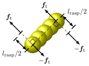
(b)

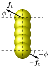
(c)

Figure 2: A bacterium as a rod-like pusher consisting of 5 point particles. (a) representation of the swimmer while it moving along $\bm{\hat{b}}$; a force-dipole ($\bm{f}_{\mathrm{r}}$ and $-\bm{f}_{\mathrm{r}}$) separated by $l_{\mathrm{rasp}}/2$ is attached to the last point particle. (b) shows the tumbling mechanism; two force-dipoles ($\bm{f}_{\mathrm{t}}$ and $-\bm{f}_{\mathrm{t}}$), each of which is separated by $l_{\mathrm{rasp}}/2$, are attached to the first and the last point particles, aligned perpendicularly to the swimmer’s long axis. (c) shows the azimuthal reorientation $\phi$ by which the direction of $\bm{f_{\mathrm{t}}}$ is defined. The dashed line through which $\phi$ is specified is arbitrarily chosen but perpendicular to the swimmer’s long axis. Note that $\bm{\hat{b}}\parallel\bm{f_{\mathrm{r}}}$ and $\bm{f_{\mathrm{r}}}\perp\bm{f_{\mathrm{t}}}$ have to be fulfilled.

II.2 Translational diffusion coefficient

Because a RT swimmer’s trajectory consists of persistent runs with sudden changes in direction, the mean-squared displacement (MSD) of such a swimmer’s trajectory is given by Lovely and Dahlquist (1975)

$$\left<\Delta r^{2}\right>=N\left<b^{2}\right>\left[\frac{1+\left(2\frac{\left<b\right>^{2}}{\left<b^{2}\right>}-1\right)\left<\cos\theta\right>}{1-\left<\cos\theta\right>}\right],$$ (11)

where $\left<b\right>$ is the average persistent running length, $\left<b^{2}\right>$ the second moment of running lengths $b$, and $N$ the number of persistent runs.

The time it takes for the RT swimmer to complete $N$ number of persistent runs is approximately Lovely and Dahlquist (1975) $t\approx N\left(\left<T_{\mathrm{t}}\right>+\left<T_{\mathrm{r}}\right>\right)$. Note that the subscript $k$ is omitted. Therefore, the MSD as a function of time $t$ reads

$$\left<\Delta r^{2}(t)\right>=\frac{\left<b^{2}\right>t}{\left<T_{\mathrm{t}}\right>+\left<T_{\mathrm{r}}\right>}\left[\frac{1+\left(2\frac{\left<b\right>^{2}}{\left<b^{2}\right>}-1\right)\left<\cos\theta\right>}{1-\left<\cos\theta\right>}\right].$$ (12)

Using the definition of the translational diffusion coefficient in three dimensions, i.e., $\left<\Delta r^{2}(t)\right>=6D_{\mathrm{t}}t$, one can explicitly write

$$D_{\mathrm{t}}=\frac{1}{6}\frac{\left<b^{2}\right>}{\left<T_{\mathrm{t}}\right>+\left<T_{\mathrm{r}}\right>}\left[\frac{1+\left(2\frac{\left<b\right>^{2}}{\left<b^{2}\right>}-1\right)\left<\cos\theta\right>}{1-\left<\cos\theta\right>}\right].$$ (13)

The first two moments, $\left<b\right>$ and $\left<b^{2}\right>$, can be calculated using the relations in Eqs. 3 and 5:

$$\left<b\right>=\left<T_{\mathrm{r}}\right>U_{\mathrm{s}}=(\left<T_{\mathrm{r}}\right>+\left<T_{\mathrm{t}}\right>)U_{\mathrm{eff}},$$ (14)

$$\left<b^{2}\right>=2(\left<T_{\mathrm{r}}\right>U_{\mathrm{s}})^{2}=2((\left<T_{\mathrm{r}}\right>+\left<T_{\mathrm{t}}\right>)U_{\mathrm{eff}})^{2},$$ (15)

where $U_{\mathrm{eff}}$ is the effective swimming speed of the RT swimmer:

$$U_{\mathrm{eff}}=\frac{\left<T_{\mathrm{r}}\right>}{\left<T_{\mathrm{r}}\right>+\left<T_{\mathrm{t}}\right>}U_{\mathrm{s}}$$ (16)

with $U_{\mathrm{s}}$ being the swimming speed.

The three expressions above further simplify the determining equation for the translational diffusion coefficient:

$$D_{\mathrm{t}} =\frac{U_{\mathrm{eff}}^{2}}{3}(\left<T_{\mathrm{r}}\right>+\left<T_{\mathrm{t}}\right>)\left[\frac{1}{1-\left<\cos\theta\right>}\right]$$ (17)

$$=\frac{U_{\mathrm{eff}}^{2}}{3}T_{\mathrm{c}},$$

where $T_{\mathrm{c}}$ is the correlation time, defined as

$$T_{\mathrm{c}}\equiv\frac{\left<T_{\mathrm{r}}\right>+\left<T_{\mathrm{t}}\right>}{1-\left<\cos\theta\right>}\overset{\text{\lx@cref{creftype~refnum}{eq:resol_cos}}}{\approx}2(\left<T_{\mathrm{r}}\right>+\left<T_{\mathrm{t}}\right>).$$ (18)

Equation 17 predicts the translational diffusion coefficient from experimentally accessible quantities. It is worth noting the following inequality:

$$T_{\mathrm{c}}\geq\left<T_{\mathrm{r}}\right>.$$ (19)

The equality holds if and only if the RT swimmer changes its direction instantaneously, i.e., $T_{\mathrm{t}}=0$, and if the reorientation distribution is symmetric, yielding $\left<\cos\theta\right>=0$.

II.3 Rotational diffusion coefficient

To obtain the rotational diffusion coefficient $D_{\mathrm{r}}$, we measure the orientational autocorrelation function during tumbles. Since we already know how the reorientation angle $\theta$ evolves in time from Eq. 7, we can easily calculate the autocorrelation function:

$$\left<\bm{\hat{b}}(t)\cdot\bm{\hat{b}}(0)\right> =\sum_{l=0}^{\infty}e^{-l(l+1)D_{\mathrm{r}}t}$$ (20)

$$\times\int_{0}^{\pi}\frac{2l+1}{2}P_{l}(\cos\theta)\sin\theta\cos\theta\mathrm{d}\theta$$

$$=e^{-2D_{\mathrm{r}}t}.$$

The orientational autocorrelation function shows an exponentially decaying behavior with the exponent being $-2D_{\mathrm{r}}$.

III Implementation

In the following we describe a momentum conserving implementation of the aforementioned run-and-tumble statistics for a hybrid MD/LB simulation within the software package ESPResSo Weik et al. (2019); Arnold et al. (2013). The lattice-Boltzmann method serves as a hydrodynamics solver Succi (2001); Krüger et al. (2017), whereas the molecular dynamics method solves Newton’s equations of swimmer’s motion. These two simulation methods are coupled via a frictional coupling scheme described in Ref. Ahlrichs and Dünweg (1999). Including hydrodynamic interactions makes our simulation scheme not only versatile as it allows us to study multiple RT swimmers without sacrificing the swimmers’ hydrodynamic interactions, but also satisfy the momentum conservation law (see below). Note that one can also exclude the hydrodynamical interactions by simply not using the LB, since our RT algorithm does not rely on the hydrodynamical interactions. The model can, therefore, be implemented also in other numerical schemes, e.g., like Langevin or Brownian MD, or Monte Carlo.

III.1 Swimmer configuration

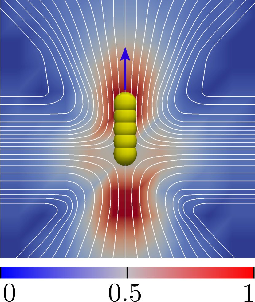
(a)

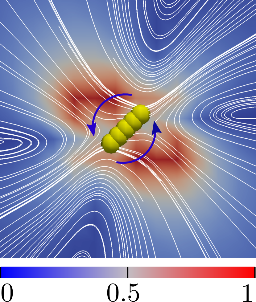
(b)

Figure 3: The induced flow field of the swimmer in the laboratory frame during (a) running, and (b) tumbling, respectively. The color map represents the normalized flow speed, and the white lines the streamlines which massless tracers would follow.

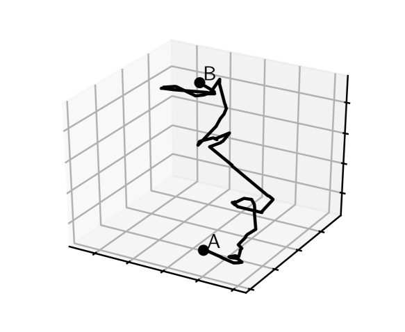
Figure 4: The trajectory of the run-and-tumble swimmer in the simulation. The point A is the starting position, and the point B is the position at time $10^{7}\tau$.

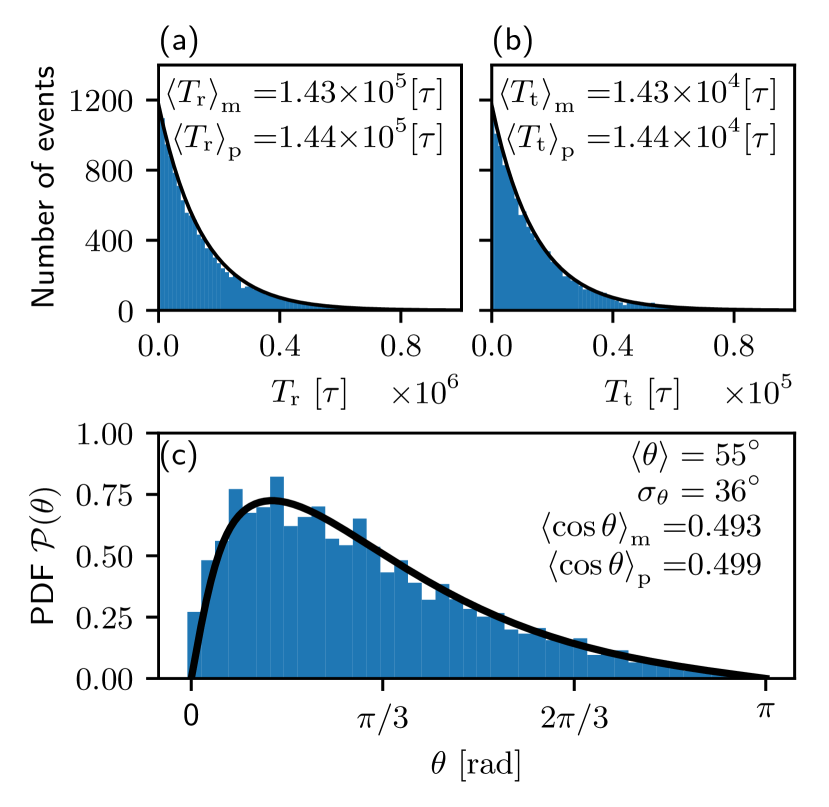
Figure 5: The durations of runs (a) and tumbles (b), and the distribution of reorientations (c). $\left<\square\right>_{\mathrm{m}}$ and $\left<\square\right>_{\mathrm{p}}$ indicate an average value that we measure and an average value that we predict from the parameters that we prescribed, respectively. The black lines represent the corresponding predicted curves.

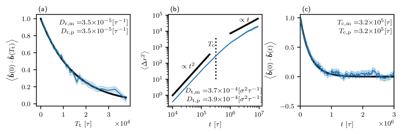
Figure 6: (a): The orientational autocorrelation as a function of tumble duration $T_{\mathrm{t}}$. The black curve is the fit from which $D_{\mathrm{r,m}}$ is taken. (b): The mean-squared displacement (MSD) of the swimmer ensemble trajectory. The black lines denote the fits for the ballistic ($\propto t^{2}$) and diffusive ($\propto t$) regimes. The translational diffusion coefficient $D_{\mathrm{t,m}}$ is obtained by a linear fit to the diffusive regime. The vertical dashed line indicates the correlation time $T_{\mathrm{c}}$. (c): The directional correlation as a function of time $t$, measuring the correlation time $T_{\mathrm{c}}$. The black curve is the fit from which to obtain $T_{\mathrm{c,m}}$. Throughout all plots, the shadowed zones covers the corresponding standard errors.

If we would couple the particle only at one point to the LB fluid we would not be able to prescribe a torque on it. Therefore we use a raspberry approach Lobaskin and Dünweg (2004); Fischer et al. (2015); de Graaf et al. (2015, 2016a). For our model we construct the swimmer as a rigid body consisting of 5 point particles. The total length of the swimmer is denoted by $l_{\mathrm{rasp}}$ as shown in Fig. 2. The effective diameter of each particle is set to be $l_{\mathrm{rasp}}/2$, which is realized through a Weeks-Chandler-Andersen interaction potential Weeks, Chandler, and Andersen (1971). The raspberry method is particularly useful for modeling arbitrarily shaped objects due to its great simplicity and versatility.

The model bacterium has now acquired some internal structure and thus two rotational degrees of freedom: rotating and precessing. Note that the swimmer still cannot experience a torque that spins it with respect to the swimmer’s long axis, which corresponds to the change in azimuthal angle $\phi$. Therefore, the change in $\phi$ happens instantaneously (see Fig. 2(c)).

A force is applied onto the swimmer during the running phase in order to model the swimming mechanism. By applying the corresponding counter-force onto the fluid at a distance of $l_{\mathrm{rasp}}/2$ the total linear momentum is conserved. These two forces thus form a force-dipole, turning the particle into a so-called pusher swimmer de Graaf et al. (2016a, b)(see Fig. 3(a)). Keep in mind that the distance between the force and counter-force, or the dipole distance, is not fixed by requiring momentum conservation alone. It is a reasonable choice to fix it somewhere within the length of the bacterias flagella, and it should not be too small since then the flow field generated by the counter-force starts affecting the dynamics of the swimmer de Graaf et al. (2016a). Therefore, we have chosen a dipole distance of $l_{\mathrm{rasp}}/2$.

Note that a force-dipole exhibits two singularities, and a swimmer experiences a repulsive hydrodynamic force by approaching another swimmer’s "tail", where the counter-force is being applied to the fluid Zöttl and Stark (2016); Winkler (2016); Spagnolie and Lauga (2012). Therefore, the effective size of the swimmer can be approximated by twice the length of the raspberry particle, that is, $l_{\mathrm{s}}\approx 2l_{\mathrm{rasp}}$.

During tumbling we attach two oppositely pointing force-dipoles at the two terminating particles of the swimmer, aligned perpendicularly to the swimmer’s long axis (see Fig. 2(b)). This always guarantees angular momentum conservation when the swimmer is tumbling, regardless of the dipole distances. Each force-dipole is, due to the same reason mentioned above, separated by $l_{\mathrm{rasp}}/2$ as well. Note that the direction of the force-dipoles on the azimuthal plain are defined by an arbitrarily chosen axis that is perpendicular to the swimmer’s long axis (see Fig. 2(c)).

The corresponding flow fields when the swimmer is running and tumbling are shown in Fig. 3. Note that the force-dipole scheme is one of the simplest representations of bacteria inducing flow fields that satisfy the momentum conservation law. Thus, we want to stress that this model only reproduces the correct far field Winkler (2016); Zöttl and Stark (2016); Spagnolie and Lauga (2012), but due to its asymmetric shape it can also be influenced hydrodynamically via flows like any similarly shaped bacterium.

III.2 Simulation parameters of the run-and-tumble algorithm

We need to set several parameters beforehand: the swimmer’s length $l_{\mathrm{s}}$, the average durations of runs $\left<T_{\mathrm{r}}\right>$ and tumbles $\left<T_{\mathrm{t}}\right>$, the Poisson time step $\delta t$, the swimming speed $U_{\mathrm{s}}$, and the rotational diffusion coefficient $D_{\mathrm{r}}$. Here, we aim to reproduce the dynamics of E. coli as closely as possible to the experimental data found in Refs. Berg and Brown (1972); Berg (1993); Saragosti, Silberzan, and Buguin (2012).

The parameters that are related to the swimmer’s running motion are subject to a (swimming) Péclet number, which is defined as Zöttl and Stark (2016); Clement et al. (2016):

$$\mathrm{Pe}=\frac{U_{\mathrm{eff}}T_{\mathrm{c}}}{l_{\mathrm{s}}}\approx\frac{2U_{\mathrm{s}}\left<T_{\mathrm{r}}\right>}{l_{\mathrm{s}}}.$$ (21)

For the sake of comparability against the experiments, we set Pe as 4.8, which is obtained from the corresponding experimental data Berg and Brown (1972); Berg (1993); Saragosti, Silberzan, and Buguin (2012) with $l_{\mathrm{s}}=10\mathrm{\mu m}$ Clement et al. (2016). Note that, however, the Péclet number can be different from one experiment to another since the quantities in Eq. 21 can show large variances.

The swimmer’s tumbling motion, on the other hand, is governed by the rotational diffusion coefficient $D_{\mathrm{r}}$ and the average tumble duration $\left<T_{\mathrm{t}}\right>$. We set $D_{\mathrm{r}}=5s^{-1}=3.5\times 10^{-5}\tau^{-1}$ and $\left<T_{\mathrm{t}}\right>=0.1s=1.44\times 10^{4}\tau$ with $\tau$ being the LB-MD time step. These values are again taken from the experiments Berg and Brown (1972); Berg (1993); Saragosti, Silberzan, and Buguin (2012); Clement et al. (2016).

The only free parameter left is the Poisson time step which defines the accuracy of the run and tumble durations. Therefore, the Poisson time step should be small compared to $\left<T_{\mathrm{t}}\right>$. However, if the Poisson time step gets smaller the simulation becomes computationally more expensive. We thus found a reasonable balance between accuracy and computational speed at $\delta t=100\tau$.

Once these parameters are determined, we iteratively apply the following scheme:

1. Draw a random number for a running duration $T_{\mathrm{r}}$ from the geometric distribution Eq. 1 whose termination rate is $q_{\mathrm{r}}$.

2. Let the swimmer run with the swimming speed $U_{\mathrm{s}}$ for $T_{\mathrm{r}}$.

3. Draw a random number for a tumbling duration $T_{\mathrm{t}}$ from the geometric distribution Eq. 1 whose termination rate is $q_{\mathrm{t}}$.

4. With the randomly drawn tumbling duration $T_{\mathrm{t}}$, draw a random number for a reorientation $\theta$ from the probability density function Eq. 7.

5. Draw a random number for an azimuthal reorientation $\phi$ from a uniform distribution that ranges $[0,2\pi]$, and make the swimmer azimuthally "spin" by $\phi$.

6. Assign the angular speed $\Omega=\theta/T_{\mathrm{t}}$ to the swimmer, and let it rotate for $T_{\mathrm{t}}$.

7. Go back to the step 1.

IV Results

We demonstrate the validity of our run-and-tumble swimmer model by analyzing the following observables: the durations of runs and tumbles, the distribution of reorientations, and the translational and rotational diffusion coefficients.

We place a swimmer in a periodic cubic box whose side length is $40\sigma$ with $\sigma$ being the diameter of a particle ($\sigma=l_{\mathrm{rasp}}/2$). The box length is chosen to be large enough such that any artifacts due to periodic boundary conditions are negligible. Initially the lattice Boltzmann fluid is set up in equilibrium. We ran 20 independent simulations for $10^{8}\tau$. To make a reasonable ensemble set, we cut each simulation into 10 blocks. We then construct the ensemble with 200 independent data sets. The chopping does not compromise the quality of the data since $10^{7}\tau$ is long enough for the system to be uncorrelated with its initial state, that is, $T_{\mathrm{c}}\ll 10^{7}\tau$. A sample for a RT trajectory is shown in Fig. 4.

We first analyze the distributions of the RT motion, and our results agree with the experimental data Berg and Brown (1972); Berg (1993). As stated in Section II.1, the duration distributions of runs and tumbles in Fig. 5a and Fig. 5b follow a Poisson statistics. The measured distribution of reorientations in Fig. 5c matches with the analytically formulated probability function (see Eq. 9).

The important remark here is the skewed distribution of reorientations, which was first discovered by Berg and Brown in 1972 Berg and Brown (1972). This is because the most probable duration of tumbles is very close to 0 as shown in Fig. 5b. This leads to the most probable reorientation to be very small as well. Consequently, the resultant distribution of reorientations is skewed to a smaller angle.

Note that, as mentioned in Section II, the Poisson time step affects the measure of $\left<\cos\theta\right>$, and our choice of the Poisson time step is 100$\tau$. With this value, we analytically predict $\left<\cos\theta\right>=0.499$ and measured $\left<\cos\theta\right>=0.493$ (see Fig. 5c). In the limit of an infinitely small Poisson time step, the expected value is $\lim\limits_{\delta t\to 0}\left<\cos\theta\right>=0.5$.

What is of equal importance as the distributions are the rotational and translational diffusion coefficients. In Fig. 6a, we display our data for the rotational diffusion coefficient $D_{\mathrm{r}}$ that turns out to be very close to the assigned value of $D_{\mathrm{r}}$. This is one of the indications that our simulation algorithm works as intended. When it comes to the translational diffusion coefficient $D_{\mathrm{t}}$, however, we have not prescribed it. $D_{\mathrm{t}}$ results solely from the ensemble of our swimmer’s trajectories. We have reproduced E. coli’s run-and-tumble motion within 5% of the relative error judging by the translation diffusion coefficient (see Fig. 6b). In addition, one can clearly see the characteristic behavior of an MSD: a ballistic regime for short times and a transition to a diffusive regime for longer times. The transition happens around the correlation time $T_{\mathrm{c}}$, which is also precisely captured by our data, as shown in Fig. 6c.

It is worth mentioning the discrepancy between the experimental results obtained by Berg and ours. He measured an average angle of $\left<\cos\theta\right>\sim 0.33$ Berg (1993), which is smaller than what we measured. We identified three possible reasons for this difference, namely the introduction of a threshold angle for reorientations in the experiment, the uncertainty in the rotational diffusion constant $D_{\mathrm{r}}$ and finally the finite frame rate of the recording device in the experiment of Berg.

V Conclusion and outlook

In summary, we have implemented an algorithm for the RT motion of a self-propelled particle coupled to a lattice-Boltzmann fluid. Furthermore we have developed an expression for the time-independent distribution of reorientations describing the RT motion of bacteria. With the help of this expression we analyzed an ensemble of RT trajectories, obtained via our LB-MD simulations of a single RT swimmer, which are prescribed by a Péclet number (Pe), a rotational diffusion coefficient ($D_{\mathrm{r}}$), an average tumble duration ($\left<T_{\mathrm{t}}\right>$), and a Poisson time step ($\delta t$).

Our RT swimmer model reproduces the real E. coli’s RT motion with excellent accuracy. Our analysis of the mean-squared displacement further demonstrates that our model provides the correct translational and rotational diffusion constants of an E. coli bacterium. Another advantage of our model over a standard Langevin implementation is that, apart from incorporating hydrodynamics, we have an explicit reorientation process of the RT motion, which reproduce nearly identical trajectories to those of E. coli.

In future investigations we will use this implementation to study the collective behavior of E. coli in various environments and under external flow conditions.

References

References

- Berg and Brown (1972) H. C. Berg and D. A. Brown, Nature 239, 500 (1972).
- Berg (1993) H. C. Berg, Random Walks in Biology (Princeton University Press, 1993).
- Ebeling, Schweitzer, and Tilch (1999) W. Ebeling, F. Schweitzer, and B. Tilch, BioSystems 49, 17 (1999).
- Elgeti and Gompper (2013) J. Elgeti and G. Gompper, Europhysics Letters 101, 48003 (2013).
- Elgeti and Gompper (2015) J. Elgeti and G. Gompper, Europhysics Letters 109, 58003 (2015).
- Ezhilan, Alonso-Matilla, and Saintillan (2015) B. Ezhilan, R. Alonso-Matilla, and D. Saintillan, Journal of Fluid Mechanics 781, R4 (2015).
- Cates and Tailleur (2013) M. E. Cates and J. Tailleur, Europhysics Letters 101, 20010 (2013).
- Cates (2012) M. E. Cates, Reports on Progress in Physics 75, 042601 (2012).
- Lighthill (1952) M. Lighthill, Communications on Pure and Applied Mathematics 5, 109 (1952).
- Blake (1971) J. Blake, Journal of Fluid Mechanics 46, 199 (1971).
- Winkler (2016) R. G. Winkler, The European Physical Journal Special Topics 225, 2079 (2016).
- Lauga (2011) E. Lauga, Soft Matter 7, 3060 (2011).
- Zöttl and Stark (2016) A. Zöttl and H. Stark, Journal of Physics: Condensed Matter 28, 253001 (2016).
- Saragosti, Silberzan, and Buguin (2012) J. Saragosti, P. Silberzan, and A. Buguin, PLOS ONE 7, e35412 (2012).
- Lovely and Dahlquist (1975) P. S. Lovely and F. Dahlquist, Journal of Theoretical Biology 50, 477 (1975).
- Dünweg and Ladd (2009) B. Dünweg and A. J. C. Ladd, in Advanced Computer Simulation Approaches for Soft Matter Sciences III, Advances in Polymer Science, Vol. 221 (Springer-Verlag Berlin, Berlin, Germany, 2009) pp. 89–166.
- Ahlrichs and Dünweg (1999) P. Ahlrichs and B. Dünweg, Journal of Chemical Physics 111, 8225 (1999).
- Krüger et al. (2017) T. Krüger, H. Kusumaatmaja, A. Kuzmin, O. Shardt, G. Silva, and E. M. Viggen, The Lattice Boltzmann Method: Principles and Practice (Springer, Cham, 2017).
- Succi (2001) S. Succi, The lattice Boltzmann equation for fluid dynamics and beyond (Oxford University Press, New York, USA, 2001).
- de Graaf et al. (2016a) J. de Graaf, H. Menke, A. J. T. M. Mathijssen, M. Fabritius, C. Holm, and T. N. Shendruk, The Journal of Chemical Physics 144, 134106 (2016a).
- de Graaf et al. (2016b) J. de Graaf, A. J. T. M. Mathijssen, M. Fabritius, H. Menke, C. Holm, and T. N. Shendruk, Soft Matter 12, 4704 (2016b).
- Weik et al. (2019) F. Weik, R. Weeber, K. Szuttor, K. Breitsprecher, J. de Graaf, M. Kuron, J. Landsgesell, H. Menke, D. Sean, and C. Holm, The European Physical Journal Special Topics 227, 1789 (2019).
- Arnold et al. (2013) A. Arnold, O. Lenz, S. Kesselheim, R. Weeber, F. Fahrenberger, D. Röhm, P. Košovan, and C. Holm, in Meshfree Methods for Partial Differential Equations VI, Lecture Notes in Computational Science and Engineering, Vol. 89, edited by M. Griebel and M. A. Schweitzer (Springer Berlin Heidelberg, 2013) pp. 1–23.
- Lobaskin and Dünweg (2004) V. Lobaskin and B. Dünweg, New Journal of Physics 6, 54 (2004).
- Fischer et al. (2015) L. P. Fischer, T. Peter, C. Holm, and J. de Graaf, The Journal of Chemical Physics 143, 084107 (2015).
- de Graaf et al. (2015) J. de Graaf, T. Peter, L. P. Fischer, and C. Holm, The Journal of Chemical Physics 143, 084108 (2015).
- Weeks, Chandler, and Andersen (1971) J. D. Weeks, D. Chandler, and H. C. Andersen, The Journal of Chemical Physics 54, 5237 (1971).
- Spagnolie and Lauga (2012) S. E. Spagnolie and E. Lauga, Journal of Fluid Mechanics 700, 105 (2012).
- Note (1) In fact, the size of swimmer is irrelevant for a single swimmer if there are no other object with which the swimmer interacts. However, this notion is still useful because a (swimming) Péclet number, describing the persistency of swimmer’s directional motion, requires a length scale (see Section III.2).
- Clement et al. (2016) E. Clement, A. Lindner, C. Douarche, and H. Auradou, The European Physical Journal Special Topics 225, 2389 (2016).