Relaxation of dynamically prepared out-of-equilibrium initial states within and beyond linear response theory

Abstract

We consider a realistic nonequilibrium protocol, where a quantum system in thermal equilibrium is suddenly subjected to an external force. Due to this force, the system is driven out of equilibrium and the expectation values of certain observables acquire a dependence on time. Eventually, upon switching off the external force, the system unitarily evolves under its own Hamiltonian and, as a consequence, the expectation values of observables equilibrate towards specific constant long-time values. Summarizing our main results, we show that, in systems which violate the eigenstate thermalization hypothesis (ETH), this long-time value exhibits an intriguing dependence on the strength of the external force. Specifically, for weak external forces, i.e., within the linear response regime, we show that expectation values thermalize to their original equilibrium values, despite the ETH being violated. In contrast, for stronger perturbations beyond linear response, the quantum system relaxes to some nonthermal value which depends on the previous nonequilibrium protocol. While we present theoretical arguments which underpin these results, we also numerically demonstrate our findings by studying the real-time dynamics of two low-dimensional quantum spin models.

I Introduction

Recent years have witnessed an increased interest in the emergence of thermodynamic behavior in closed quantum many-body systems polkovnikov2011 ; gogolin2016 ; dalessio2016 ; borgonovi2016 . At the heart of this subject lies the question if and how an isolated system, undergoing solely unitary time evolution, eventually relaxes to some long-time steady state which is compliant with the prediction of statistical mechanics, i.e., fixed by a few macroscopic parameters only.

A key approach which has been put forward to answer this question is the eigenstate thermalization hypothesis (ETH) deutsch1991 ; srednicki1994 ; rigol2005 . The ETH explains thermalization on the basis of individual eigenstates and can be formulated as an Ansatz about the matrix structure of local observables in the eigenbasis of the respective Hamiltonian. Loosely speaking, it states that for generic (nonintegrable) quantum systems, the diagonal matrix elements of local operators depend smoothly on energy. (When speaking about a violation of the ETH in the following, we generally refer to an absence of this property.) Given that the ETH is fulfilled, then, independent of the specific out-of-equilibrium initial state, the expectation values of such operators will always relax to their thermal values prescribed by the microcanonical ensemble.

While it is already hard to proof the validity of the ETH for a given model apart from numerical evidence santos2010 ; beugeling2014 ; kim2014 ; mondaini2017 ; jansen2019 ; steinigeweg2013 , there are also classes of systems which generically violate this Ansatz, with integrable and many-body-localized models basko2006 ; nandkishore2015 being the prime examples. On the one hand, due to the macroscopic number of quasi(local) conservation laws, thermalization to standard statistical ensembles is precluded in integrable models. Specifically, the long-time steady state in these systems is captured in terms of a suitable generalized Gibbs ensemble instead essler2016 ; vidmar2016 . On the other hand, many-body localization can arise in a system with strong disorder. Due to this disorder, transport ceases and the system defies thermalization on indefinite time scales abanin2018 .

Nevertheless, even for systems which violate the ETH (i.e. eigenstate expectation values of local operators are not smooth), there still exist out-of-equilibrium initial states for which observables dynamically equilibrate to their thermal values at long times, see e.g. rigol2012 ; shiraishi2017 . In fact, from a mathematical point of view, these states even form the majority of all possible initial states. Specifically, this statement is also related to the notion of typicality popescu2006 ; goldstein2006 ; reimann2007 . One central result of typicality is the fact that the overwhelming majority (Haar measure) of quantum states within some energy shell yields expectation values of observables very close to the full microcanonical ensemble lloydPhd ; gemmer2004 . Or to rephrase, quantum states with visible nonequilibrium properties are mathematically rare. Remarkably, from this set of rare nonequilibrium initial states, the majority will, at long times, again exhibit expectation values close to the respective equilibrium value, given some mild conditions on the dynamics reimann2008 that are entirely unrelated to the ETH ikeda2011 ; riera2012 ; reimann2010 ; reimann2015 . It is an intriguing and open question whether actual (experimentally realizable) out-of-equilibrium initial states fall into this larger subset of all possible nonequilibrium states, or if the ETH is indeed a physically necessary condition for thermalization, see also Refs. bartsch2017 ; depalma2015 ; reimann2018 . We will explore this question by proposing a specific class of initial states which can be tuned close to and far away from equilibrium.

We consider a realistic nonequilibrium protocol, where a quantum system in thermal equilibrium is suddenly subjected to an external force. Due to this force, the system is driven out of equilibrium and the expectation values of certain observables acquire a dependence on time. Eventually, upon switching off the external force, the system unitarily evolves under its own Hamiltonian and, as a consequence, the expectation values of observables equilibrate towards specific constant long-time values. Summarizing our main results, we unveil that, in systems which violate the ETH, this long-time value exhibits an intriguing dependence on the strength of the external force. Specifically, for weak external forces, i.e., within the validity regime of linear response theory (LRT), we show that expectation values thermalize to their original equilibrium values, despite the ETH being violated. In contrast, for stronger perturbations beyond linear response, the quantum system relaxes to some nonthermal value which depends on the previous nonequilibrium protocol. Moreover, for nonintegrable systems which obey the ETH, we illustrate that the system thermalizes for all initial conditions, both within and beyond the linear response regime. Our findings exemplify that (apart from the LRT regime) the ETH is indeed a physically necessary condition for initial-state-independent relaxation and thermalization in realistic situations.

This paper is structured as follows. In Sec. II, we introduce and discuss the nonequilibrium protocol which is considered in this paper. In Sec. III, we then present numerical results for two quantum lattice models which corroborate our findings. We conclude and summarize in Sec. IV.

II Nonequilibrium Dynamics

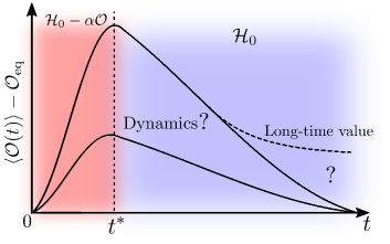
Figure 1: (Color online) Sketch of the nonequilibrium setup. For times $t<t^{\ast}$ the system evolves w.r.t. a perturbed Hamiltonian ${\cal H}_{0}-\alpha{\cal O}$. Depending on the magnitude of $\alpha$, the expectation value $\langle{\cal O}(t)\rangle$ can be driven close to or far away from its equilibrium value ${\cal O}_{\text{eq}}$. For times $t>t^{\ast}$ the system evolves with respect to ${\cal H}_{0}$. We study how the long-time value $\langle{\cal O}(t\to\infty)\rangle$ depends on the perturbation strength $\alpha$.

II.1 General protocol

Let us consider a quantum system in thermal equilibrium, i.e., at time $t=0$ it is described by a canonical density matrix,

$$\rho(0)=\rho_{\text{eq}}=\frac{e^{-\beta{\cal H}_{0}}}{{\cal Z}_{0}}\ ,$$ (1)

where ${\cal Z}_{0}=\text{Tr}[\exp(-\beta{\cal H}_{0})]$ is the partition function, $\beta=1/T$ is the inverse temperature, and ${\cal H}_{0}$ denotes the Hamiltonian of the (unperturbed) quantum system. Next, we consider a nonequilibrium protocol where an external static force of strength $\alpha$ is suddenly switched on at time $t=0$, and switched off again at $t=t^{\ast}$. For times $t<t^{\ast}$, this external force acts on the quantum system, giving rise to an additional operator ${\cal O}$ (conjugated to the force) within the Hamiltonian. Thus, the full (time-dependent) Hamiltonian ${\cal H}_{t}$ of the nonequilibrium protocol takes on the form

$${\cal H}_{t}=\begin{cases}{\cal H}_{0}-\alpha{\cal O}\ ,&0<t<t^{\ast}\\ {\cal H}_{0}\ ,&t>t^{\ast}\end{cases}\ .$$ (2)

The combination of external force and quantum system is considered as being isolated from its environment, i.e., the initial equilibrium state $\rho(0)$ evolves unitarily in time according to the von-Neumann equation, and $\rho(t)$ is given by

$$\rho(t)=\begin{cases}e^{-i({\cal H}_{0}-\alpha{\cal O})t}\rho(0)e^{i({\cal H}_{0}-\alpha{\cal O})t}\ ,&0<t<t^{\ast}\\ e^{-i{\cal H}_{0}(t-t^{\ast})}\rho(t^{\ast})e^{i{\cal H}_{0}(t-t^{\ast})}\ ,&t>t^{\ast}\end{cases}\ .$$ (3)

In the following, we will be interested in the dynamics of the same observable ${\cal O}$ which is used to perturb the system. While at time $t=0$, ${\cal O}$ takes on its equilibrium value $\langle{\cal O}(0)\rangle={\cal O}_{\text{eq}}$, the expectation value $\langle{\cal O}(t)\rangle$ acquires a time dependence due to the driving by the external force (assuming $[{\cal O},{\cal H}_{0}]\neq 0$). Specifically, for any time $t\geq 0$, $\langle{\cal O}(t)\rangle$ reads

$$\langle{\cal O}(t)\rangle=\text{Tr}[\rho(t){\cal O}]\ ,$$ (4)

where $\rho(t)$ is the out-of-equilibrium state in Eq. (3). Clearly, the time dependence of $\langle{\cal O}(t)\rangle$ can be manifold. Naively, one might expect a scenario as sketched in Fig. 1. For times $t\leq t^{\ast}$, the expectation value $\langle{\cal O}(t)\rangle$ starts increasing with a growth rate depending on the strength of the perturbation $\alpha$. The value of $\langle{\cal O}(t)\rangle$ at time $t=t^{\ast}$ is here denoted by

$$\langle{\cal O}(t^{\ast})\rangle={\cal O}^{\ast}\ .$$ (5)

Subsequently, for $t>t^{\ast}$, $\langle{\cal O}(t)\rangle$ evolves w.r.t. the unperturbed Hamiltonian ${\cal H}_{0}$ and might relax back to ${\cal O}_{\text{eq}}$, or potentially also to some other long-time value,

$$\langle{\cal O}(t\to\infty)\rangle={\cal O}^{\infty}\ .$$ (6)

Note that while the mere process of equilibration can be shown under very little assumptions on ${\cal H}_{0},{\cal O}$ reimann2008 ; short2011 , the present paper is concerned with the question of thermalization. In particular, we address the questions (i) how ${\cal O}^{\infty}$ depends on the strength of the perturbation $\alpha$, and (ii) how this dependence is affected by the validity or breakdown of the eigenstate thermalization hypothesis.

II.2 Linear response regime

Let us now discuss the nonequilibrium protocol outlined above in more detail. In fact, in the regime of small external forces, the time dependence of $\langle{\cal O}(t)\rangle$ can be simplified considerably. According to linear response theory, the dynamics of $\langle{\cal O}(t)\rangle$ in this regime follows as kubo1991

$$\langle{\cal O}(t)\rangle-{\cal O}_{\text{eq}}=\alpha\int_{0}^{t^{\ast}}\phi(t-t^{\prime})\ {\text{d}}t^{\prime},\$$ (7)

where we have exploited that the external force $\alpha(t)=\alpha$ is constant and only acts for $t\in[0,t^{\ast}]$. Moreover, the function $\phi(t)=-\beta\frac{\text{d}}{\text{d}t}(\Delta{\cal O};\Delta{\cal O}(t))$ in Eq. (7) is given in terms of a Kubo scalar product kubo1991 ,

$$\phi(t)=-\frac{\text{d}}{\text{d}t}\int_{0}^{\beta}\text{Tr}\left[e^{\lambda{\cal H}_{0}}\Delta{\cal O}e^{-\lambda{\cal H}_{0}}\Delta{\cal O}(t)\rho_{\text{eq}}\right]{\text{d}}\lambda\ ,$$ (8)

where $\Delta{\cal O}={\cal O}-{\cal O}_{\text{eq}}$ and ${\cal O}(t)=e^{i\mathcal{H}_{0}t}{\cal O}e^{-i\mathcal{H}_{0}t}$. Starting from Eqs. (7) and (8), let us now scrutinize the long-time dynamics $\langle{\cal O}(t\to\infty)\rangle$. To this end, we first define $\chi(t)=\beta(\Delta{\cal O};\Delta{\cal O}(t))$, such that $\phi(t)=-\text{d}\chi(t)/\text{d}t$ Note0 . Next, let $t_{\text{eq}}$ be the time for which $\chi(t)$ equilibrates, i.e, $\chi(t)$ is essentially time-independent for $t>t_{\text{eq}}$,

$$\chi(t>t_{\text{eq}})\approx\overline{\chi}=\text{const}\ .$$ (9)

Moreover, let $\tau>t_{\text{eq}}$ be a (long) time which is chosen such that $\tau-t_{\text{eq}}>t^{\ast}$. In view of Eq. (7), the expectation value $\langle{\cal O}(\tau)\rangle$ then follows as

$$\langle{\cal O}(\tau)\rangle-{\cal O}_{\text{eq}} =\alpha\int_{0}^{t^{\ast}}\phi(\tau-t)\ \text{d}t$$ (10)

$$=\alpha\big{[}\chi(\tau)-\chi(\tau-t^{\ast})\big{]}\approx 0\ ,$$ (11)

since $\chi(\tau)=\chi(\tau-t^{\ast})\approx\overline{\chi}$, cf. Eq. (9). In particular, for a fixed value of $t^{\ast}$, there always exists a time $\tau$ with $\tau-t_{\text{eq}}>t^{\ast}$ for which Eq. (11) is valid, and in the limit $\tau\to\infty$ we can generally write

$${\cal O}^{\infty}-{\cal O}_{\text{eq}}\approx 0.$$ (12)

Thus, for small external forces within the validity regime of LRT, the system relaxes back to its original equilibrium value. Remarkably, this statement only requires equilibration of $\chi(t)$, and is therefore expected to hold for a large number of systems [and initial states of the form (1) and (3)], even if the ETH is violated. This is a first important result of the present paper.

However, the expression given in Eq. (7) is only valid for small external forces, and terms of the order $\alpha^{2},\alpha^{3},\dots$ can become important when $\alpha$ is increased. As a consequence, Eq. (12) can break down, and it is an intriguing question how ${\cal O}^{\infty}$ changes for values of $\alpha$ beyond LRT. This transition between small and large values of $\alpha$ will be in the focus of our numerical study in the upcoming section.

III Numerical Analysis

Let us now numerically study the nonequilibrium protocol outlined in Sec. II. First, we introduce our models in Sec. III.1. Then, we describe our numerical approach in Sec. III.2, before presenting our results in Sec. III.3.

III.1 Models

III.1.1 The XXZ chain

As a first example, we consider the one-dimensional anisotropic Heisenberg model (XXZ chain) with periodic boundary conditions. The model is described by the Hamiltonian

$${\cal H}_{0}=J\sum_{l=1}^{L}\left(S_{l}^{x}S_{l+1}^{x}+S_{l}^{y}S_{l+1}^{y}+\Delta S_{l}^{z}S_{l+1}^{z}\right)\ ,$$ (13)

where the $S_{l}^{\mu}$, $\mu=x,y,z$ are spin-$1/2$ operators at lattice site $l$, $J=1$ is the antiferromagnetic exchange constant, $L$ is the number of lattice sites, and $\Delta\geq 0$ denotes the exchange anisotropy in the $z$-direction.

As an observable for our nonequilibrium protocol, we here choose the spin current ${\cal J}$, which can be defined in terms of a lattice continuity equation and takes on the well-known form heidrichmeisner2007 ,

$${\cal J}=J\sum_{l=1}^{L}\left(S_{l}^{x}S_{l+1}^{y}-S_{l}^{y}S_{l+1}^{x}\right)\ .$$ (14)

Thus, as outlined in Eqs. (2) and (3), the system evolves w.r.t. ${\cal H}_{0}-\alpha{\cal J}$ for $t<t^{\ast}$, and we study the relaxation of $\langle{\cal J}(t)\rangle$ for long times. Note that, while a specific force for this particular operator is probably difficult to realize in an experiment, this numerical example nevertheless nicely illustrates the main results of the present paper.

The XXZ chain defined in Eq. (13) is integrable in terms of the Bethe Ansatz for all values of $\Delta$ sutherlandBook . For the particular case of $\Delta=0$, it can be mapped to a model of free spinless fermions with ${\cal J}$ being exactly conserved. Moreover, while $[{\cal J},{\cal H}_{0}]\neq 0$ for all $\Delta\neq 0$, it has been shown that ${\cal J}$ is at least partially conserved for anisotropies $\Delta<1$ zotos1999 ; prosen2013 ; urichuk2019 . For the purpose of this paper, we therefore choose $\Delta=0.5$. An explicit finite-size scaling, in order to confirm that the ETH is indeed violated for this choice of parameters, can be found, e.g., in Ref. steinigeweg2013 .

As a comparison, it is furthermore instructive to study the dynamics of ${\cal J}$ also in a case where the ETH is valid. To this end, we consider an integrability-breaking next-nearest neighbor interaction of strength $\Delta^{\prime}$, i.e., the new Hamiltonian of the system then reads,

$${\cal H}_{0}^{\prime}={\cal H}_{0}+J\Delta^{\prime}\sum_{l}S_{l}^{z}S_{l+2}^{z}\ .$$ (15)

Note that the specific form of the spin current (14) importantly remains unaffected. In particular, we here choose $\Delta=\Delta^{\prime}=0.5$ for which quantum chaos occurs rigol2010 , and the ETH is expected to hold steinigeweg2013 ; richter2018_3 .

III.1.2 The asymmetric spin ladder

As a second example, we study an asymmetric and anisotropic spin-$1/2$ ladder. The Hamiltonian of the spin ladder has a leg part ${\cal H}_{\parallel}$ and a rung part ${\cal H}_{\perp}$,

$${\cal H}_{0}={\cal H}_{\parallel}+{\cal H}_{\perp}\ ,$$ (16)

where ${\cal H}_{\parallel}$ essentially consists of two separate XXZ chains, cf. Eq. (13), with different lengths $L_{1},L_{2}$, exchange constant $J_{\parallel}$, and open boundary conditions. Moreover, these two chains are then connected according to

$${\cal H}_{\perp}=J_{\perp}\sum_{l=1}^{L_{1}}S_{l,1}^{x}S_{l,2}^{x}+S_{l,1}^{y}S_{l,2}^{y}+\Delta S_{l,1}^{z}S_{l,2}^{z}\ ,$$ (17)

where we have chosen $L_{1}<L_{2}$ without loss of generality. The total number of lattice sites is $L=L_{1}+L_{2}$. Based on a finite-size analysis of level statistics and of fluctuations of diagonal matrix elements, the spin ladder (16) has been shown to undergo a transition between a chaotic phase and an ETH-violating phase for large interchain couplings $J_{\perp}/J_{\parallel}\gtrsim 4$ khodja2015 ; khodja2016 . Since our goal is not to thoroughly screen all parameter regimes, but rather to numerically illustrate the physical mechanisms discussed in Sec. II, we here choose two representative points in parameter space. Namely, for the chaotic phase we choose $J_{\perp}=0.2$, whereas for the nonchaotic regime we have $J_{\perp}=4.2$. Moreover, we fix $J_{\parallel}=1$ and $\Delta=0.1$, cf. Refs. bartsch2017 ; khodja2016 .

Furthermore, as an observable, we study the magnetization difference between the two legs of the spin ladder,

$${\cal M}=\sum_{l=1}^{L_{1}}S_{l,1}^{z}-\sum_{l=1}^{L_{2}}S_{l,2}^{z}\ .$$ (18)

In particular, this magnetization difference allows for an intuitive understanding of our nonequilibrium protocol. Specifically, the external force of strength $\alpha$ would correspond to a magnetic field which is directed in positive $z$-direction on the first leg, and in negative $z$-direction on the second leg.

III.2 Dynamical quantum typicality

In order to evaluate time-dependent expectation values $\langle{\cal O}(t)\rangle$ for large system sizes (outside the range of exact diagonalization), we here rely on an efficient pure-state approach based on the concept of dynamical quantum typicality (DQT) hams2000 ; iitaka2003 ; sugiura2013 ; elsayed2013 ; steinigeweg2014 . Within this concept, a single (randomly drawn) pure quantum state can imitate the properties of the full density matrix. Specifically, in order to calculate the expectation value $\langle{\cal O}(t)\rangle$, the trace $\text{Tr}[\rho(t){\cal O}]$ is replaced by a simple scalar product,

$$\langle{\cal O}(t)\rangle=\bra{\psi_{\beta}(t)}{\cal O}\ket{\psi_{\beta}(t)}+\epsilon\ .$$ (19)

Here, $\ket{\psi_{\beta}(t)}$ denotes the unitarily time-evolved state [analogous to Eq. (3)], and $\ket{\psi_{\beta}(0)}$ is a typical state at inverse temperature $\beta$ sugiura2013 ; steinigeweg2014 ,

$$\ket{\psi_{\beta}(0)}=\frac{e^{-\beta{\cal H}_{0}/2}\ket{\varphi}}{\sqrt{\bra{\varphi}e^{-\beta{\cal H}_{0}}\ket{\varphi}}}\ ,\quad\ket{\varphi}=\sum_{k=1}^{d}c_{k}\ket{\varphi_{k}}\ ,$$ (20)

where the reference pure state $\ket{\varphi}$ would correspond to infinite temperature. In particular, the complex coefficients $c_{k}$ in Eq. (20) are randomly drawn from a Gaussian distribution with zero mean (Haar measure) bartsch2009 , and the sum runs over the full Hilbert space with dimension $d=2^{L}$ and basis states $\ket{\varphi_{k}}$ (in practice, we here choose the Ising basis). Note that the statistical error $\epsilon=\epsilon(\ket{\varphi})$ in Eq. (19) scales as $\epsilon\propto 1/\sqrt{d_{\text{eff}}}$, where $d_{\text{eff}}={\cal Z}_{0}/e^{-\beta E_{0}}$ is the effective dimension of the Hilbert space, and $E_{0}$ is the ground-state energy of ${\cal H}_{0}$ hams2000 ; bartsch2009 ; elsayed2013 ; steinigeweg2014 ; steinigeweg2015 . Thus, $\epsilon$ decreases exponentially with system size, and the typicality approximation becomes very accurate if $L$ is sufficiently large (especially for small values of $\beta$) Note2 . See also Ref. endo2018 for a recent study of linear and nonlinear response using typical pure states, as well as Refs. bartsch2017 ; richter2018 ; richter2018_2 ; richter2019 for a different but related nonequilibrium setup.

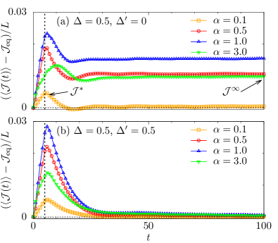
Figure 2: (Color online) (a) Expectation value $(\langle{\cal J}(t)\rangle-{\cal J}_{\text{eq}})/L$ for the XXZ chain with $\Delta=0.5$, $\Delta^{\prime}=0$. Data is shown for various strengths of the external force $\alpha$, which acts up to times $t^{\ast}=5$ (as indicated by the dashed vertical line). The horizontal dashed line signals zero. (b) Analogous data as in panel (a), but now for the nonintegrable model with $\Delta=\Delta^{\prime}=0.5$. The other parameters are $L=24$ and $\beta=1$.

The main numerical advantage of Eq. (19) stems from the fact that instead of density matrices, one only has to deal with pure states. Particularly, in order to construct the states $\ket{\psi_{\beta}(0)}$ and $\ket{\psi_{\beta}(t)}$, the exponentials $e^{-\beta\mathcal{H}_{0}/2}$ or $e^{-i\mathcal{H}t}$ can be efficiently evaluated by iteratively solving the imaginary- or real-time Schrödinger equation, respectively. While various sophisticated methods are available for this task, such as Trotter decompositions deReadt2006 , Chebychev polynomials dobrovitski2003 ; weisse2006 , and Krylov subspace techniques varma2017 , we here rely on a fourth order Runge-Kutta scheme where the discrete time step is chosen short enough to guarantee negligible numerical errors elsayed2013 ; steinigeweg2014 . Such iterator methods, in combination with the sparseness of generic few-body operators, enable the treatment of Hilbert-space dimensions significantly larger compared to standard exact diagonalization steinigeweg2014 ; steinigeweg2015 ; richter2019_1 ; richter2019_2 .

III.3 Results

We now present our numerical results. Note that our data are calculated for a single temperature $\beta=1$ only. In particular, we have chosen this moderate temperature since it (i) is low enough such that the system can be driven out of equilibrium with reasonable effort Note1 , but (ii) is high enough to ensure that finite-size effects and numerical errors are small Note2 . Moreover, while details of the nonequilibrium dynamics can of course vary with temperature, the overall picture is expected to apply to all values of $\beta$, i.e., there will be a regime of sufficiently small $\alpha$ where LRT holds, as well as a regime of large $\alpha$ where LRT breaks down. Naturally, the notion of small and large can depend on the chosen temperature $T$. (Note that there can exist cases where LRT breaks down at $T=0$ gamayun2014 )

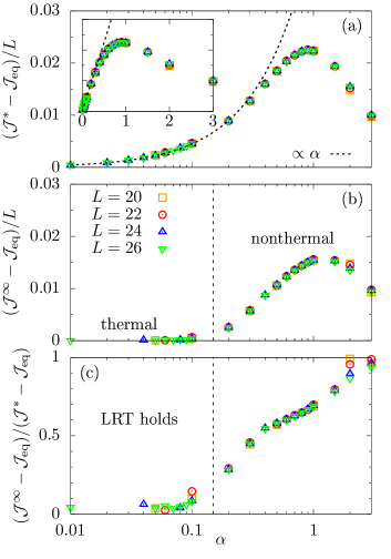
Figure 3: (Color online) (a) $({\cal J}^{\ast}-{\cal J}_{\text{eq}})/L$ versus perturbation strength $\alpha$. Inset shows same data, but with linear $\alpha$-axis. (b) $({\cal J}^{\infty}-{\cal J}_{\text{eq}})/L$ versus $\alpha$. (c) Ratio $({\cal J}^{\infty}-{\cal J}_{\text{eq}})/({\cal J}^{\ast}-{\cal J}_{\text{eq}})$ versus $\alpha$. Data are shown for different system sizes $L=20,\dots,26$. Note that ${\cal J}^{\infty}$ is extracted at time $t=100\gg t^{\ast}$. The other parameters are $\Delta=0.5$, $\Delta^{\prime}=0$, and $\beta=1$.

III.3.1 The XXZ chain

To begin with, we consider the spin current ${\cal J}$ in the XXZ chain as introduced in Sec. III.1.1. In order to get a general impression how the dynamics of ${\cal J}$ depends on the strength of the external force, the expectation value $\langle{\cal J}(t)\rangle$ is exemplarily shown in Figs. 2 (a) and (b) for different values $\alpha=0.1,0.5,1,3$, and a single system size $L=24$, both for the integrable as well as the nonintegrable model. The nonequilibrium protocol is here designed in such a way that the external force acts for times $0<t<5$, i.e., we have $t^{\ast}=5$, as indicated by the dashed vertical line.

First, for short times $t<t^{\ast}$, we observe in all cases a monotonic increase of $\langle{\cal J}(t)\rangle$ with time, consistent with the fact that the system is driven out of equilibrium. Specifically, comparing data for $\alpha=0.1,0.5$ and $\alpha=1$, we moreover find that the growth rate of $\langle{\cal J}(t)\rangle$ increases with $\alpha$, such that ${\cal J}^{\ast}=\langle{\cal J}(t^{\ast})\rangle$ is larger for larger $\alpha$. Quite counterintuitively, however, we find that for an even stronger $\alpha=3$, the value of ${\cal J}^{\ast}$ is actually smaller compared to $\alpha=0.5,1$. In fact, for this large value of $\alpha$, the maximum of $\langle{\cal J}(t)\rangle$ in the integrable model [Fig. 2 (a)] is shifted to times $t\approx 10$ which is considerably beyond $t^{\ast}$, as if the system does not notice that the external force has been already removed. Such a qualitative change in the dynamics clearly indicates a transition from linear to nonlinear response when going from smaller to larger values of $\alpha$.

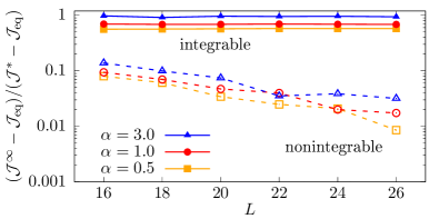
Figure 4: (Color online) Ratio $({\cal J}^{\infty}-{\cal J}_{\text{eq}})/({\cal J}^{\ast}-{\cal J}_{\text{eq}})$ versus system size $L$ for different values of $\alpha$ (outside the LRT regime), obtained by diagonalization ($L=16$) and DQT ($L\geq 18$). Data are shown for the integrable model with $\Delta=0.5$, $\Delta^{\prime}=0$, and the nonintegrable model with $\Delta=\Delta^{\prime}=0.5$. Since the value of ${\cal J}^{\infty}$ is extracted at the finite time $t=100$, the data have to be understood as upper bounds to the true infinite-time limit (especially for the nonintegrable model)

. We have $\beta=1$ in all cases.

Next, concerning the dynamics for $t>t^{\ast}$ in Fig. 2 (a), we observe that after reaching its maximum (approximately at $t^{\ast}$), $\langle{\cal J}(t)\rangle$ starts to decrease again, before eventually equilibrating to an approximately constant value ${\cal J}^{\infty}$ at long times. While ${\cal J}^{\infty}-{\cal J}_{\text{eq}}\approx 0$ in the case of $\alpha=0.1$ (see also further discussion below), we find that ${\cal J}^{\infty}-{\cal J}_{\text{eq}}$ clearly takes on a nonzero value for larger $\alpha$. In the following, we will analyze this dependence of ${\cal J}^{\infty}$ (and in particular the dependence of the ratio ${\cal J}^{\infty}/{\cal J}^{\ast}$) on the strength of the external force $\alpha$ in the integrable model in more detail. In contrast, for the nonintegrable model shown in Fig. 2 (b), we find that ${\cal J}^{\infty}-{\cal J}_{\text{eq}}$ is very small and appears to vanish irrespective of the specific value of $\alpha$ (although the considered time scales might still be too short).

In Figs. 3 (a)-(c), the three quantities ${\cal J}^{\ast}-{\cal J}_{\text{eq}}$, ${\cal J}^{\infty}-{\cal J}_{\text{eq}}$, and $({\cal J}^{\infty}-{\cal J}_{\text{eq}})/({\cal J}^{\ast}-{\cal J}_{\text{eq}})$ are depicted for integrable chains ($\Delta=0.5$, $\Delta^{\prime}=0$) with different system sizes $L\geq 20$ and a number of $\alpha$ ranging from $\alpha=0.01$ up to $\alpha=3$. Note that the $\alpha$-axis has a logarithmic scale. First of all, as shown in Fig. 3 (a), we observe a linear increase of ${\cal J}^{\ast}$ for small $\alpha\lesssim 0.2$, as expected from linear response theory. (This fact can also be seen in the inset of Fig. 3 (a) which has a linear axis.) Moreover, for $\alpha\gtrsim 0.2$, deviations from this linear growth become apparent, and for even larger $\alpha\gtrsim 1$, one finds that ${\cal J}^{\ast}$ decreases with increasing $\alpha$, consistent with our discussion in the context of Fig. 2. As a side remark, while ${\cal J}^{\ast}$ is not necessarily the maximum of $\langle{\cal J}(t)\rangle$, cf. Fig. 2 (a), the overall findings would be very similar if we plotted this maximum instead of ${\cal J}^{\ast}$.

Next, Fig. 3 (b) shows the long-time value ${\cal J}^{\infty}$, which is extracted from the real-time dynamics at time $t=100\gg t^{\ast}$. On the one hand, for small $\alpha\lesssim 0.2$, we observe that ${\cal J}^{\infty}-{\cal J}_{\text{eq}}\approx 0$, which is in good agreement with the linear regime found in Fig. 3 (a), and consistent with our discussion in Sec. II. (The fact that ${\cal J}^{\infty}-{\cal J}_{\text{eq}}$ is not strictly zero can be explained by (i) the finite system size $L$, (ii) the finite time $t=100$ to extract ${\cal J}^{\infty}$, and (iii) the statistical error $\epsilon$ of the typicality approximation.) On the other hand, for $\alpha\gtrsim 0.2$, we find that ${\cal J}^{\infty}$ takes on a nonthermal value. Eventually, let us emphasize that the data shown in Figs. 3 (a) and (b) are normalized to the respective system size $L$, resulting in a convincing data collapse for all values of $\alpha$ and $L$ shown. This indicates that our findings are not just caused by trivial finite-size effects.

Since both ${\cal J}^{\ast}-{\cal J}_{\text{eq}}$ and ${\cal J}^{\infty}-{\cal J}_{\text{eq}}$ become small for $\alpha\to 0$, it is instructive to study their ratio

$${\cal R}=({\cal J}^{\infty}-{\cal J}_{\text{eq}})/({\cal J}^{\ast}-{\cal J}_{\text{eq}})\ .$$ (21)

As can be seen in Fig. 3 (c), this ratio is very small for $\alpha\lesssim 0.2$, and drastically changes its behavior for $\alpha\gtrsim 0.2$. This clearly confirms our earlier findings from Fig. 3 (b). Namely, for small $\alpha$ within the validity regime of LRT, ${\cal J}$ relaxes back to its original equilibrium independent of the specific out-of-equilibrium state. In contrast, for stronger $\alpha$ beyond LRT, ${\cal J}$ equilibrates at a nonthermal value ${\cal J}^{\infty}$, and in particular, this ${\cal J}^{\infty}$ clearly depends on the previous nonequilibrium protocol, i.e., on the specific value of $\alpha$. This is an important result of the present paper. (See also Ref. kennes2017 for similar findings.)

While Fig. 3 already shows data for different system sizes $L$, let us perform a detailed finite-size scaling for selected values of $\alpha$. In this context, it is especially instructive to study how our findings change if an integrability-breaking next-nearest neighbor interaction is considered. To this end, Fig. 4 shows the ratio ${\cal R}$, cf. Eq. (21), as a function of $L$ for $\alpha=0.5,1,3$ (outside the LRT regime). As already discussed above, we find that ${\cal R}$ essentially does not exhibit any dependence on system size for the integrable (ETH-violating) model. Thus, even in the thermodynamic limit $L\to\infty$, the system does not thermalize at long times. In contrast, if we consider the nonintegrable model where the ETH holds steinigeweg2013 , we observe that ${\cal R}$ clearly decreases with increasing $L$ for all values of $\alpha$ shown here, and will likely vanish for $L\to\infty$. This exemplifies that, for our realistic nonequilibrium protocol, the ETH is indeed a necessary condition for thermalization (at least for $\alpha$ beyond LRT). This is another important result.

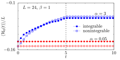
Figure 5: (Color online) Expectation value of the energy density $\langle{\cal H}_{0}(t)\rangle/L$ for the integrable ($\Delta=0.5$, $\Delta^{\prime}=0$, filled symbols), and the nonintegrable ($\Delta=\Delta^{\prime}=0.5$, open symbols) XXZ chain. Data are shown for a small value $\alpha=0.05$ and large value $\alpha=3$ of the external force. The other parameters are $L=24$ and $\beta=1$.

Eventually, let us note that due to the driving by the external force, the system experiences a change of the internal energy mierzejewski2011 . This heating is monitored in Fig. 5, where we show $\langle{\cal H}_{0}(t)\rangle/L$ for the XXZ chain, both for the integrable and the nonintegrable model. Moreover, we depict data for a small external force $\alpha$ within LRT, and a strong external force beyond LRT. On the one hand, for a small $\alpha=0.05$, we observe that $\langle{\cal H}_{0}(t)\rangle$ is essentially constant over the whole time window $t<t^{\ast}$. (Note that for times $t>t^{\ast}$, $\langle{\cal H}_{0}(t)\rangle$ is trivially time-independent.) On the other hand, for a large $\alpha=3$, we find that $\langle{\cal H}_{0}(t)\rangle$ monotonically increases, such that $\langle{\cal H}_{0}(t^{\ast})\rangle\neq\langle{\cal H}_{0}(0)\rangle$. In this context, it is important to stress that the nonthermal long-time value ${\cal J}^{\infty}$ shown in Fig. 3 (b) for $\alpha\gtrsim 0.2$ cannot be explained by this change of the internal energy, i.e., it is not just a new thermal value at a different effective temperature. In particular, it follows from symmetry considerations that the (isolated) XXZ chain cannot carry a nonzero spin current in equilibrium, such that ${\cal J}_{\text{eq}}=0$ for all energy densities steinigeweg2013 . In fact, the nonthermal long-time value ${\cal J}^{\infty}$ in Fig. 3 (b) is a direct consequence of the violation of the ETH and can be related to the fluctuations of the diagonal matrix elements of ${\cal J}$ steinigeweg2013 ; richter2018 .

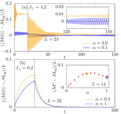
Figure 6: (Color online) (a) Expectation value of the magnetization difference $(\langle{\cal M}(t)\rangle-{\cal M}_{\text{eq}})/L$ in the strong-coupling regime with $J_{\perp}=4.2$, exemplarily shown for $\alpha=0.1,3$ and system size $L_{1}=8$, $L_{2}=15$. Inset shows same data, but only for the time window $120<t<150$. (b) Analogous data as in panel (a), but now for the chaotic regime with $J_{\perp}=0.2$ and $\alpha=0.5,1$. The inset shows the dependence of ${\cal M}^{\ast}$ on $\alpha$, obtained by diagonalization for $L_{1}=5$, $L_{2}=9$ [see Fig. 7 (a) for data at $J_{\perp}=4.2$]. The small circles indicate the values of ${\cal M}^{\ast}$ and $\alpha$ which correspond to the two curves shown in the main panel. The vertical dashed lines in (a) and (b) indicate the duration of the external perturbation $t^{\ast}=20,100$. The other parameters are, $J_{\parallel}=1$, $\Delta=0.1$, and $\beta=1$.

III.3.2 The asymmetric spin ladder

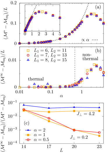
Figure 7: (Color online) (a) $({\cal M}^{\ast}-{\cal M}_{\text{eq}})/L$ versus $\alpha$ for $L=17,20,23$ [see key in (b) for details] and $J_{\perp}=4.2$. Inset shows same data, but with linear $\alpha$-axis. (b) $({\cal M}^{\infty}-{\cal M}_{\text{eq}})/L$ versus $\alpha$ for $J_{\perp}=4.2$. (c) Ratio $({\cal M}^{\infty}-{\cal M}_{\text{eq}})/({\cal M}^{\ast}-{\cal M}_{\text{eq}})$ versus system size $L$ for $\alpha=0.5,1,2$. Data is shown for both, strong interchain coupling $J_{\perp}=4.2$ where the ETH is violated, and weak $J_{\perp}=0.2$ where the system is chaotic. The other parameters are $J_{\parallel}=1$, $\Delta=0.1$, and $\beta=1$.

To corroborate our findings further, let us now also study the asymmetric spin ladder introduced in Sec. III.1.2. In Figs. 6 (a) and (b), we again exemplarily depict the nonequilibrium dynamics of the magnetization difference $\langle{\cal M}(t)\rangle$ for different perturbation strengths $\alpha$, both for the ETH-violating regime ($J_{\perp}=4.2$) and the chaotic regime ($J_{\perp}=0.2$). In case of the former [Fig. 6 (a)], we find that the magnetization difference exhibits a sudden drop at $t=t^{\ast}$. Moreover, due to the rather strong rung coupling, $\langle{\cal M}(t)\rangle$ shows pronounced oscillations which also persist up to the longest time $t=150$ considered. Due to this oscillatory behavior, we extract both ${\cal M}^{\ast}$ and ${\cal M}^{\infty}$ as an average over a suitably chosen time window. In contrast, for the chaotic regime in Fig. 6 (b), the dynamics is considerably slower such that we choose a larger $t^{\ast}=100$ and extract ${\cal M}^{\infty}$ around $t\approx 500$.

Next, Figs. 7 (a) and 7 (b) show $({\cal M}^{\ast}-{\cal M}_{\text{eq}})/L$ and $({\cal M}^{\infty}-{\cal M}_{\text{eq}})/L$ versus $\alpha$ for different system sizes $L$ and $J_{\perp}=4.2$. Analogous to our discussion of the spin current in Fig. 3 (a), we again find a regime of small $\alpha\lesssim 0.6$ where ${\cal M}^{\ast}$ grows linearly with $\alpha$. Furthermore, for $\alpha\gtrsim 2$ we also observe the counterintuitive phenomenon that ${\cal M}^{\ast}$ decreases although the external force becomes stronger.

Concerning the long-time value shown in Fig. 7 (b), we find ${\cal M}^{\infty}-{\cal M}_{\text{eq}}\approx 0$ for $\alpha\lesssim 0.6$, as well as a monotonic growth of ${\cal M}^{\infty}$ for $\alpha\gtrsim 0.6$. Thus, although the overall effect is considerably weaker in the case of the spin ladder (see also Note3 ), Fig. 7 (b) confirms our previous findings from Figs. 2 to 4. In particular, we again can clearly identify two separate regimes, i.e., a first regime for weak $\alpha$ where $\langle{\cal M}(t)\rangle$ takes on its thermal value at long times, and a second regime for larger $\alpha$ where LRT breaks down and ${\cal M}^{\infty}$ is nonthermal.

Since qualitatively similar, we have omitted in Fig. 7 the analogous panel (c) compared to Fig. 4. Instead, Fig. 7 (c) presents a finite-size scaling of ${\cal R}_{\cal M}=({\cal M}^{\infty}-{\cal M}_{\text{eq}})/({\cal M}^{\ast}-{\cal M}_{\text{eq}})$ for different values of the external force $\alpha$. In particular, we also show data for the chaotic region of the parameter space with smaller rung couping $J_{\perp}=0.2$, where the ETH is expected to apply bartsch2017 ; khodja2015 ; khodja2016 . [Note however, that the LRT regime is found to be smaller in the chaotic regime, see inset of Fig. 6 (b)]. On the one hand, for strong ${\cal J}_{\perp}=4.2$, we find that ${\cal R}_{\cal M}$ is practically independent of the system size. On the other hand, for ${\cal J}_{\perp}=0.2$, we find that ${\cal R}_{\cal M}$ decreases approximately exponentially for increasing $L$. Thus, the validity of the ETH in the chaotic regime ensures thermalization at long times, independent of the specific initial state.

IV Conclusion

To summarize, we have studied a particular type of nonequilibrium protocol where a quantum system in thermal equilibrium is suddenly subjected to an external force which drives the system out of equilibrium. Eventually, this external force is switched off again, and the system evolves under its own (unperturbed) Hamiltonian.

As main results, we have shown that, in systems which violate the ETH, the long-time value of observables exhibits an intriguing dependence on the strength of the external force. Specifically, for weak external forces, i.e., within the linear response regime, we unveiled that expectation values thermalize to their original equilibrium values, despite the ETH being violated. In contrast, for stronger perturbations beyond linear response, the quantum system relaxes to some nonthermal value which depends on the previous nonequilibrium protocol.

We have substantiated our results by numerically studying the real-time dynamics of observables in two low-dimensional quantum lattice models: (i) the spin current in the one-dimensional XXZ model, and (ii) the magnetization difference between the two legs in an asymmetric spin ladder. In particular, we have employed an efficient pure-state approach in order to study large systems, and to demonstrate that our findings do not depend on system size. In this context, we have also demonstrated that in the case of a nonintegrable model, the system relaxes back to thermal equilibrium (also for far-from-equilibrium initial states).

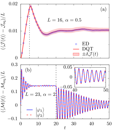
Figure 8: (Color online) (a) Comparison of $\langle{\cal J}(t)\rangle$ obtained by the typicality approach, cf. Eq. (19), and by exact diagonalization for $L=16$. DQT data are averaged over $N=100$ samples, and the shaded area indicates sample-to-sample fluctuations, cf. Eq. (22). Note that the error of the mean scales as $\delta\overline{{\cal J}(t)}\propto\delta{\cal J}(t)/\sqrt{N}$. (b) $\langle{\cal M}(t)\rangle$ obtained from two different realizations of the pure state $\ket{\varphi}$, cf. Eq. (20), for a ladder with $L_{1}=8$, $L_{2}=15$. We have $\beta=1$ in all cases.

On the one hand, our findings exemplify that the ETH is indeed a physically necessary condition for initial-state-independent relaxation and thermalization in realistic situations. On the other hand, and almost paradoxically, our nonequilibrium protocol at the same time exhibits the intriguing property that systems can thermalize for initial states within the LRT regime, despite the ETH being violated.

Promising directions of research include, e.g., the consideration of other time-dependent external perturbations, a more thorough investigation of the dependence on temperature, as well as the study of many-body localized systems within this nonequilibrium protocol.

Acknowledgements

This work has been funded by the Deutsche Forschungsgemeinschaft (DFG) - Grants No. 397107022 (GE 1657/3-1), No. 397067869 (STE 2243/3-1), No. 355031190 - within the DFG Research Unit FOR 2692.

Appendix A Accuracy of the pure-state approach

In order to demonstrate that dynamical quantum typicality [Eq. (19)] indeed provides an accurate numerical approach to study nonequilibrium dynamics, Fig. 8 (a) shows a comparison of $\langle{\cal J}(t)\rangle$ with exact diagonalization data for a small system of size $L=16$. One clearly observes that both methods agree convincingly with each other for all times shown here. In particular, the DQT data are averaged over $N$ different random realizations of the pure state $\ket{\varphi}$, cf. Eq. (20), and the shaded area indicates the standard deviation of sample-to-sample fluctuations richter2018 ,

$$\delta{\cal J}(t)=\left[\sum_{n=1}^{N}\frac{\langle{\cal J}(t)\rangle^{2}_{(n)}}{N}-\left(\sum_{n=1}^{N}\frac{\langle{\cal J}(t)\rangle_{(n)}}{N}\right)^{2}\right]^{\tfrac{1}{2}}\ .$$ (22)

The error of the mean scales as $\delta\overline{{\cal J}(t)}\propto\delta{\cal J}(t)/\sqrt{N}$, and is well-controlled for the choice of $N=100$ used here. As outlined below Eq. (20), the accuracy of the pure-state approach is expected to improve even further for increasing Hilbert-space dimension. Therefore, averaging becomes less important for increasing $L$, and the data for $L\geq 20$ shown in Figs. 2 to 4 essentially represents the exact dynamics. Note that data for $L\geq 22$ in Fig. 4 is calculated from a single pure state $N=1$ only. Note further that the data in Fig. 7 has been obtained by averaging over $N=300$ ($L=17$), $N=100$ ($L=20$), and $N=1$ ($L=23$) states. We expect the small fluctuations in Fig. 7 to vanish if $N$ is increased further.

Another convenient means to demonstrate the smallness of the statistical error $\epsilon$ is the direct comparison of data resulting from two different instances of the typical state $\ket{\varphi}$. Such a comparison is shown in Fig. 8 (b) for the magnetization difference $\langle{\cal M}(t)\rangle$ in a spin ladder with $L=23$ sites. One observes that the data resulting from $\ket{\varphi_{1}}$ and $\ket{\varphi_{2}}$ coincide very well with each other, illustrating that Eq. (19) indeed provides a reliable tool to obtain quantum many-body dynamics for large system sizes.

References

- (1) A. Polkovnikov, K. Sengupta, A. Silva, and M. Vengalattore, Rev. Mod. Phys. 83, 863 (2011).
- (2) C. Gogolin and J. Eisert, Rep. Prog. Phys. 79, 056001 (2016).
- (3) L. D’Alessio, Y. Kafri, A. Polkovnikov, and M. Rigol, Adv. Phys. 65, 239 (2016).
- (4) F. Borgonovi, F. M. Izrailev, L. F. Santos, and V. G. Zelevinsky, Phys. Rep. 626, 1 (2016).
- (5) J. M. Deutsch, Phys. Rev. A 43, 2046 (1991).
- (6) M. Srednicki, Phys. Rev. E 50, 888 (1994).
- (7) M. Rigol, V. Dunjko, and M. Olshanii, Nature 452, 854 (2008).
- (8) L. F. Santos and M. Rigol, Phys. Rev. E 82, 031130 (2010).
- (9) W. Beugeling, R. Moessner, and M. Haque, Phys. Rev. E 89, 042112 (2014).
- (10) H. Kim, T. N. Ikeda, D. A. Huse, Phys. Rev. E 90, 052105 (2014).
- (11) R. Mondaini and M. Rigol, Phys. Rev. E 96, 012157 (2017).
- (12) D. Jansen, J. Stolpp, L. Vidmar, and F. Heidrich-Meisner, Phys. Rev. B 99, 155130 (2019).
- (13) R. Steinigeweg, J. Herbrych, and P. Prelovšek, Phys. Rev. E 87, 012118 (2013).
- (14) D. M. Basko, I. L. Aleiner, and B. L. Altshuler, Ann. Phys. 321, 1126 (2006).
- (15) R. Nandkishore and D. A. Huse, Annu. Rev. Condens. Matter Phys. 6, 15 (2015).
- (16) F. H. L. Essler and M. Fagotti, J. Stat. Mech. 2016, 064002 (2016).
- (17) L. Vidmar and M. Rigol, J. Stat. Mech. 2016, 064007 (2016).
- (18) D. A. Abanin, E. Altman, I. Bloch, and M. Serbyn, Rev. Mod. Phys. 91, 021001 (2019).
- (19) M. Rigol and M. Srednicki, Phys. Rev. Lett. 108, 110601 (2012).
- (20) N. Shiraishi and T. Mori, Phys. Rev. Lett. 119, 030601 (2017).
- (21) S. Popescu, A. J. Short, and A. Winter, Nat. Phys. 2, 754 (2006).
- (22) S. Goldstein, J. L. Lebowitz, R. Tumulka, and N. Zanghì, Phys. Rev. Lett. 96, 050403 (2006).
- (23) P. Reimann, Phys. Rev. Lett. 99, 160404 (2007).
- (24) S. Lloyd, Ph.D. Thesis, The Rockefeller University (1988), Chapter 3, arXiv:1307.0378.
- (25) J. Gemmer, M. Michel, and G. Mahler, Quantum Thermodynamics (Springer, Berlin, 2004).
- (26) P. Reimann, Phys. Rev. Lett. 101, 190403 (2008).
- (27) T. N. Ikeda, Y. Watanabe, and M. Ueda, Phys. Rev. E 84, 021130 (2011).
- (28) A. Riera, C. Gogolin, and J. Eisert, Phys. Rev. Lett. 108, 080402 (2012).
- (29) P. Reimann, New. J. Phys. 12, 055027 (2010).
- (30) P. Reimann, Phys. Rev. Lett. 115, 010403 (2015).
- (31) C. Bartsch and J. Gemmer, EPL (Europhys. Lett.) 118, 10006 (2017).
- (32) G. De Palma, A. Serafini, V. Giovannetti, and M. Cramer, Phys. Rev. Lett. 115, 220401 (2015).
- (33) P. Reimann, Phys. Rev. Lett. 120, 230601 (2018).
- (34) A. J. Short, New J. Phys. 13, 053009 (2011).
- (35) R. Kubo, M. Toda, and N. Hashitsume, Statistical Physics II: Nonequilibrium Statistical Mechanics, Solid-State Sciences 31 (Springer, Berlin, 1991).
- (36) The definition of is only fixed up to a constant offset, which is however irrelevant for our considerations.
- (37) F. Heidrich-Meisner, A. Honecker, and W. Brenig, Eur. Phys. J. Spec. Top. 151, 135 (2007).
- (38) B. Sutherland, Beautiful Models: 70 Years of Exactly Solved Quantum Many-body Problems (World Scientific Publishing, Singapore, 2004).
- (39) X. Zotos, Phys. Rev. Lett. 82, 1764 (1999).
- (40) T. Prosen and E. Ilievski, Phys. Rev. Lett. 111, 057203 (2013).
- (41) A. Urichuk, Y. Oez, A. Klümper, and J. Sirker, SciPost Phys. 6, 005 (2019).
- (42) M. Rigol and L. F. Santos, Phys. Rev. A 82, 011604(R) (2010).
- (43) J. Richter, F. Jin, H. De Raedt, K. Michielsen, J. Gemmer, and R. Steinigeweg, Phys. Rev. B 97, 174430 (2018).
- (44) A. Khodja, R. Steinigeweg, and J. Gemmer, Phys. Rev. E 91, 012120 (2015).
- (45) A. Khodja, D. Schmidtke, and J. Gemmer, Phys. Rev. E 93, 042101 (2016).
- (46) A. Hams and H. De Raedt, Phys. Rev. E 62, 4365 (2000).
- (47) T. Iitaka and T. Ebisuzaki, Phys. Rev. Lett. 90, 047203 (2003).
- (48) S. Sugiura and A. Shimizu, Phys. Rev. Lett. 111, 010401 (2013).
- (49) T. A. Elsayed and B. V. Fine, Phys. Rev. Lett. 110, 070404 (2013).
- (50) R. Steinigeweg, J. Gemmer, and W. Brenig, Phys. Rev. Lett. 112, 120601 (2014).
- (51) C. Bartsch and J. Gemmer, Phys. Rev. Lett. 102, 110403 (2009).
- (52) R. Steinigeweg, J. Gemmer, and W. Brenig, Phys. Rev. B 91, 104404 (2015).
- (53) For more details on the accuracy of our pure-state approach, see Appendix A.
- (54) H. Endo, C. Hotta, and A. Shimizu, Phys. Rev. Lett. 121, 220601 (2018).
- (55) J. Richter, J. Herbrych, and R. Steinigeweg, Phys. Rev. B 98, 134302 (2018).
- (56) J. Richter, J. Gemmer, and R. Steinigeweg, Phys. Rev. E 99, 050104(R) (2019).
- (57) J. Richter and R. Steinigeweg, Phys. Rev. E 99, 012114 (2019).
- (58) H. De Raedt and K. Michielsen, in Handbook of Theoretical and Computational Nanotechnology (American Scientific Publishers, Los Angeles, 2006).
- (59) V. V. Dobrovitski and H. De Raedt, Phys. Rev. E 67, 056702 (2003).
- (60) A. Weiße, G. Wellein, A. Alvermann, and H. Fehske, Rev. Mod. Phys. 78, 275 (2006).
- (61) V. K. Varma, A. Lerose, F. Pietracaprina, J. Goold, and A. Scardicchio, J. Stat. Mech. 2017 053101 (2017).
- (62) J. Richter and R. Steinigeweg, Phys. Rev. B 99, 094419 (2019).
- (63) J. Richter, F. Jin, L. Knipschild, J. Herbrych, H. De Raedt, K. Michielsen, J. Gemmer, and R. Steinigeweg, Phys. Rev. B 99, 144422 (2019).
- (64) As becomes evident from Eqs. (7) and (8), a smaller value of leads to a smaller response of the system for fixed value of .
- (65) O. Gamayun, O. Lychkovskiy, and V. Cheianov, Phys. Rev. E 90, 032132 (2014).
- (66) D. M. Kennes, J. C. Pommerening, J. Diekmann, C. Karrasch, and V. Meden, Phys. Rev. B 95, 035147 (2017).
- (67) M. Mierzejewski, J. Bonča, and P. Prelovšek, Phys. Rev. Lett. 107, 126601 (2011).
- (68) In fact, the relaxation towards a nonthermal value in the spin ladder is considerably more pronounced in a different nonequilibrium setup, see Ref. bartsch2017 .