The SAMI Galaxy Survey: Stellar population radial gradients in early-type galaxies

Abstract

We study the internal radial gradients of the stellar populations in a sample comprising 522 early-type galaxies (ETGs) from the SAMI (Sydney- AAO Multi-object Integral field spectrograph) Galaxy Survey. We stack the spectra of individual spaxels in radial bins, and derive basic stellar population properties: total metallicity ([Z/H]), [Mg/Fe], [C/Fe] and age. The radial gradient ($\nabla$) and central value of the fits (evaluated at R_e/4) are compared against a set of six possible drivers of the trends. We find that velocity dispersion ($\sigma$) – or, equivalently gravitational potential – is the dominant driver of the chemical composition gradients. Surface mass density is also correlated with the trends, especially with stellar age. The decrease of $\nabla$[Mg/Fe] with increasing $\sigma$ is contrasted by a rather shallow dependence of $\nabla$[Z/H] with $\sigma$ (although this radial gradient is overall rather steep). This result, along with a shallow age slope at the massive end, imposes stringent constraints on the progenitors of the populations that contribute to the formation of the outer envelopes of ETGs. The SAMI sample is split between a ‘field’ sample and a cluster sample. Only weak environment-related differences are found, most notably a stronger dependence of central total metallicity ([Z/H]_e4) with $\sigma$, along with a marginal trend of $\nabla$[Z/H] to steepen in cluster galaxies, a result that is not followed by [Mg/Fe]. The results presented here serve as constraints on numerical models of the formation and evolution of ETGs.

1 Introduction

Radial gradients of the chemical composition of the stellar populations of early-type galaxies (ETGs) encode valuable information about their build-up process (Larson, 1974). At present, the 2-stage formation scenario (e.g. Oser et al., 2010) constitutes a simplified yet insightful description of galaxy formation, especially at the massive end. In this framework, the stellar content of galaxies is split into an in-situ component, typically formed during the early collapse of the gas in the fledgling halo, followed by subsequent merging events in which stars, previously formed ex-situ, are supplied by infalling satellite galaxies. Subsequent in-situ formation is also possible via accretion and cooling of gas. In massive ETGs this separation allows us to propose a simplified scenario consisting of an early and intense phase during which a massive core is formed, along with a later accretion phase contributed by mergers. The stellar populations of massive ETGs are mostly old, enabling us to cleanly split their formation history into a core, formed in-situ at early times, and an envelope, produced by the later, ex-situ, phase.

The presence of massive, nearly quiescent cores at high redshift (z$\sim$2–3, see, e.g., Daddi et al., 2005; Trujillo et al., 2006; van Dokkum et al., 2008) suggests that a single in-situ phase is not capable of producing the massive ETGs we see today, and radial variations within ETGs can be exploited to understand the role of the ex-situ phase (e.g., Lackner et al., 2012; Hirschmann et al., 2015). Moreover, variations between field and cluster environments are expected since the latter represents an “accelerated” version of the former, as higher density regions collapse earlier.

This paper looks for clues in the formation of ETGs via intrinsic radial gradients of the underlying stellar populations. The advent of surveys based on Integral Field Spectroscopy has transformed the field of galaxy evolution (SAURON, ATLAS^3D, SAMI, CALIFA, MaNGA, Bacon et al., 2001; Cappellari et al., 2011; Croom et al., 2012; Sánchez et al., 2012; Bundy et al., 2015) enabling spatially resolved studies of all information accessible to spectroscopy. Vast amounts of information are encoded into the datacubes that are now routinely studied to explore the dynamical state and chemical properties of the stellar and gaseous phases of galaxies.

Differences between the in-situ and ex-situ components will be present not only in the stellar kinematics at large radii, but also in the stellar population properties. The longer dynamical timescales in the outer envelopes of galaxies imply that these regions fare better at preserving information related to the past merger history. Radial gradients in age and chemical composition reveal variations in the star formation histories (see, e.g., Greene et al., 2015; González-Delgado et al., 2015), including properties such as the stellar initial mass function (IMF, e.g., La Barbera et al., 2016), that reflect a fundamentally different mode of star formation during the early in-situ phase.

Simulations also reveal important signatures in population gradients. At large radii, the stellar content appears to be predominantly driven by the accretion of incoming satellite galaxies. Computer models of galaxy formation that include feedback prescriptions show that a substantial contribution from winds is needed to account for the steep metallicity gradients observed (Hirschmann et al., 2015). The Illustris ETGs feature steeper metallicity profiles when their mass assembly history is less extended (Cook et al., 2016). In principle, the steepest gradients should be expected in an orderly monolithic collapse, while mergers would act towards washing out these gradients.

Figure 1: Sample of SAMI early-type galaxies studied in this paper, showing the effective radius (R_e) against velocity dispersion ($\sigma$, left) and stellar mass (M_s, right), both shown on a logarithmic scale. The sample is split between GAMA-selected galaxies (blue crosses, representing field and group ETGs) and cluster galaxies (red circles).

The population gradients measured in a volume-limited sample of 95 massive early-type galaxies from the MASSIVE survey found a strong trend of stellar age and [Mg/Fe] with velocity dispersion, contrasting with a weaker correlation when stellar mass is considered (Greene et al., 2015). This behaviour would suggest that galaxies with high velocity dispersion are more efficient at transforming gas into stars. However, this trend disappears at larger radii ($\sim$1–1.5 R_e), suggesting a complex contribution of stellar populations in the outer regions, as they are formed ex-situ from a range of merging satellites. Boardman et al. (2017) found that the kinematics in a sample of 12 ETGs, detected in HI, did not show any variations out to three effective radii, supporting the idea that these galaxies have not undergone dry major merging at late times. However, the IFU data revealed substantial population gradients consistent with some level of interaction in recent times. More recently, Martín-Navarro et al. (2018) explored a sample of 45 ETGs from the CALIFA IFU survey, finding significant radial gradients of metallicity, that increase with velocity dispersion. In contrast, no gradient was detected with respect to [Mg/Fe] (also note Sánchez-Blázquez et al. 2014 for a comparative study in disks).

Figure 2: Distribution of ETG sample sizes, showing from left to right, the effective radius and outermost radial bin – in units of the Point Spread Function (PSF) – and the ratio of the two. The radial extent of the PSF is taken at the Half Width at Half-Maximum, individually for each galaxy. The sample is split between GAMA-selected galaxies (blue crosses, representing field and group ETGs) and cluster galaxies (red circles).

Goddard et al. (2017) presented an analysis of population gradients in a large sample of 721 galaxies from the SDSS-IV MaNGA survey, covering a wide range of stellar mass and morphology. Their results concerning the subsample of early-type galaxies reveal small age gradients, and negative metallicity gradients, without any significant correlation with galaxy environment (various definitions of environment were presented, namely nearest neighbours, gravitational tidal strength and a central/satellite split). Such a result is at odds with the trends presented in the SDSS-based Spider sample of ETGs, which suggested significantly younger ages in centrals (La Barbera et al., 2014), and variation in population radial gradients with environment (La Barbera et al., 2011). Although the stellar populations of ETGs are found to strongly correlate with velocity dispersion (see, e.g. Bernardi et al., 2003), or a similar “local” observable, environment-related variations are also found – at fixed velocity dispersion – using different samples and methods (Weinmann et al., 2006; Rogers et al., 2010; Peng et al., 2010; Smith et al., 2012; La Barbera et al., 2014). In this regard, the SAMI survey provides a unique set to probe environment-related trends, as, by construction, it comprises galaxies in a field environment – selected from the Galaxy and Mass Assembly survey, GAMA (Driver et al., 2011) – and a cluster environment (targeting eight low-redshift clusters, Owers et al., 2017).

This paper focuses on the analysis of the radial gradients found in the chemical composition and age of the stellar populations of early-type galaxies. We will characterize the trends with respect to a number of local drivers of the star formation and chemical enrichment processes, as well as consider variations with respect to environment (cluster vs field/group). Section 2 presents our working sample of SAMI early-type galaxies, and Section 3 describes the procedure followed to extract the stellar population parameters. The derivation of radial gradients is outlined in Section 4. Our results are presented in Section 5, and the interpretation of the trends, both regarding the general sample and the separation of the trends with respect to environment, are discussed in Section 6. A concluding summary is given in Section 7.

Figure 3: Illustration of the methodology applied to correct the contribution of the Point Spread Function (PSF) in the derivation of radial gradients. The left panels show a test case adopting a predefined model. The contours follow the elliptical bins used to derive the radial measurements. A model of the parameter $y=0.8-0.2($R/arcsec$)$ is imposed, and the observed PSF parameters are used to convolve the original model (leftmost panel) into an observed one, shown in the adjacent panel. The panel on the right shows the individual spaxel data (in grey), the radially binned data (with error bars corresponding to the RMS scatter) and the retrieved best fit for a linear model $y=\alpha+\beta($R/arcsec$)$ (dashed line) with slope $\beta=-0.201\pm 0.018$. A naive fit (not taking into account the PSF) produces a shallower slope (dotted line, $\beta=-0.182$). The inset shows the distribution of parameters from the MCMC sampler.

2 Early-type galaxy sample

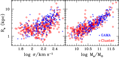
This work is based on data taken by the Sydney Australian-Astronomical-Observatory Multi-object Integral-Field-Spectrograph (SAMI). The development of hexabundle technology (Bland-Hawthorn et al., 2011; Bryant et al., 2014) enabled a generation of versatile Integral Field Units (IFU) such as SAMI. Our starting sample comprises all galaxies classified with an early-type morphology within the SAMI Galaxy Survey (Croom et al., 2012). This survey consists of spectroscopic observations of $\sim$3,600 galaxies taken with the SAMI IFU at the 3.9 m Anglo-Australian Telescope. The SAMI Galaxy Survey is described in Bryant et al. (2015), with additional details of the cluster sample in Owers et al. (2017). The full sample was visually inspected and morphologically classified as described in Cortese et al. (2016). Galaxies were first divided into spiral/non-spiral based on the presence of spiral arms or strong, regular dust features, then further subdivided based on other morphological features. We selected all galaxies classified as having a visual morphological type of E, E/S0 or S0. Our SAMI/ETG sample comprises 522 systems, split into 234 ETGs from the GAMA survey (i.e. in a field/group environment) and 288 ETGs in clusters. The sample covers a wide range of mass and size, and extends over a redshift window z=[0.013,0.095], with a median value z_M=0.053. Fig. 1 shows the distribution with respect to velocity dispersion ($\sigma$, left) and stellar mass (M_s, right), both on a log scale. Note the difference in logarithmic range (0.5 dex in $\sigma$ and 1.5 dex in M_s), and the scatter of the mean relationship, apparently larger in velocity dispersion. Although no substantial bias is apparent between GAMA and cluster galaxies, in Section 5.2 we will construct subsamples that remove any potential systematic caused by the sample selection.

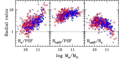
For each galaxy, we stack individual spaxel spectra in radial bins following the elliptical isophotes, as provided in the SAMI datacubes (Scott et al., 2018). A correction regarding the rotation velocity is applied independently to each spaxel – derived from the kinematics analysis (van de Sande et al., 2017) – to “align” all spectra to a common rest frame, before stacking the spaxel data corresponding to the same radial bin. Typically, the data have between 3 and 5 radial bins available. Fig. 2 shows a comparison of the radial extent of the observations as a function of stellar mass – R_LAST represents the radial extent of the outermost radial bin. The Point Spread Function (PSF), measured for each galaxy by the observation of a star in the same field, is quantified by the Half-Width at Half-Maximum (HWHM), to compare it on equal terms with galaxy radii. The median of the ratio R_LAST/R_e is 2.2. All radii are quoted as circularized values: R${}_{e}=\sqrt{a_{e}b_{e}}$, and the effective radii are retrieved from Sérsic fits to the surface brightness profile (see Kelvin et al. 2012 and Owers et al. 2018 for details).

3 Extracting population parameters

In order to analyze the spectra, we rely on Simple Stellar Population (SSP) model predictions from Vazdekis et al. (2015, hereafter $\alpha$-MILES). The $\alpha$-MILES SSPs are based on the MILES stellar library, applying corrections from theoretical models of stellar atmospheres to produce synthetic spectra of old- and intermediate-age stellar populations at 2.51 Å (FWHM) spectral resolution, with varying total metallicity ($\rm[Z/H]$), IMF, and $\rm[\alpha/Fe]$ abundance ratios. For the present work, we use models based on the BaSTI (instead of the Padova) isochrones, as these are computed at both [Mg/Fe]=0 (scaled-solar) and [Mg/Fe]=+0.4. We use SSPs with metallicities [Z/H]={$-0.96$, $-0.66$, $-0.35$, $-0.25$, $+0.06$, $+0.15$, $+0.26$}, ages from 1 to 14 Gyr (with a 1 Gyr sampling), and a Kroupa Universal IMF. Line-strength predictions from the $\alpha$-MILES models are linearly interpolated over a three-dimensional grid, with 100 equally-spaced steps in both age and metallicity, and 175 steps in [Mg/Fe]. A linear extrapolation is applied to extend the metallicity range up to $+0.5$ dex, and to probe the [Mg/Fe] range between $-0.15$ and $+0.7$ dex. However, we note that only in 5.9% (1.9%) of the cases it was necessary to invoke this extrapolation to obtain best-fit values of the stellar populations in [Z/H] ([Mg/Fe]).

For each SAMI spectrum, we estimated stellar population properties, namely age, metallicity ($\rm[Z/H]$), and $\rm[Mg/Fe]$, by minimizing the standard $\chi^{2}$ statistic, namely:

$$\rm\chi^{2}=\sum_{i}\left(\frac{O_{i}-M_{i}}{\sigma_{i}}\right)^{2},$$ (1)

where the index $\rm i$ runs over a selected set of spectral indices, O_i(M_i) are the observed (model) line-strengths, and $\sigma_{i}$ are the measurement errors of O_i. We considered different sets of spectral indices, including two combinations of Balmer lines: either $\rm H\beta_{o}$ only, or both $\rm H\beta_{o}$ and $\rm H\gamma_{F}$. For each set of Balmer lines we included all possible permutations of Fe indices, out of $\rm Fe4383$, $\rm Fe5270$, and $\rm Fe5335$. In each case, we included $\rm Mgb5170$, as it is required to constrain both metallicity and [Mg/Fe]. These indices are typically measured as an equivalent width (EW), namely:

$${\rm EW}\equiv\int_{\lambda_{1}}^{\lambda_{2}}\left[1-\frac{\Phi(\lambda)}{\Phi_{C}(\lambda)}\right],$$ (2)

where $\lambda_{1}$ and $\lambda_{2}$ define the central window of the spectral feature, $\Phi(\lambda)$ denotes the spectrum under study and $\Phi_{C}(\lambda)$ is the pseudo-continuum, given as a straight line connecting a blue and a red sideband that straddle the central feature. The uncertainty of the index is obtained by propagating the corresponding uncertainty in the observed spectrum. The central, blue and red sidebands follow the standard definition, and are taken from Trager et al. (1998), except for $\rm H\beta_{o}$, defined in Cervantes & Vazdekis (2009). For each spectrum, all model indices were computed after smoothing the $\alpha$-MILES SSPs to match its effective broadening (instrumental resolution and velocity dispersion). The amount of broadening was estimated with pPXF (Cappellari & Emsellem, 2004), performing spectral fitting in the rest-frame window 4,030–5,380 Å, that include all the spectral features targeted here. For each set of indices, we determine the best-fitting stellar population properties by minimizing Eq. 1 over the interpolated grid of $\alpha$-MILES SSP line strengths (with varying age, $\rm[Z/H]$, and $\rm[Mg/Fe]$). The parameter uncertainties are derived following a Monte Carlo approach, producing realizations of all indices when Gaussian noise, consistent with the uncertainty, is added to the line strengths.

Figure 4: Linear regression to the radial gradients (bottom panels) and the intercept at $\sigma$=200 km s^-1(top) of the (from left to right) total metallicity, [Mg/Fe] and [C/Fe]. A typical error bar of an individual measurement is shown in each panel, corresponding to the median of the uncertainties in each case. The best fit results are shown as solid blue (red) lines for the GAMA (cluster) subsample, shown as blue crosses (red open circles).

In order to account for nebular contamination in the Balmer lines, we correct the $\rm H\beta_{o}$ and $\rm H\gamma_{F}$ line-strengths with a similar procedure to that described in La Barbera et al. (2013). We estimated the excess of flux in the line with respect to a combination of two SSPs, multiplied by a polynomial, giving the best fit in the $\rm H\beta_{o}$ ($\rm H\gamma_{F}$) spectral region, 4,830–4,890 Å (4,310–4,370 Å), after excluding the absorption trough. The emission correction uncertainty was obtained by varying the degree, $N_{p}$, of the multiplicative polynomial in the fits (from $N_{p}=5$ to $11$), taking the standard deviation of the estimated emission corrections. The correction of $\rm H\beta_{o}$ turned out to be significant for $\sim 8\,\%$ of the SAMI spectra, with a median value of 0.2 Å. Since the nebular contamination of $\rm H\gamma_{F}$ is usually less significant than that on $\rm H\beta_{o}$, we only needed to correct $\rm H\gamma_{F}$ in $\sim$1% of the spectra.

Figure 5: Distribution of retrieved slopes in a synthetic set of data with the same error distribution of the observed values of [Z/H], enforcing a relation [Z/H]=$c\log\sigma_{200}$, with $c=-0.2$ for the GAMA sample (blue) and $c=+0.2$ for the cluster sample (red). See text for details.

Table 1: Details of the homogeneous samples defined with respect to the possible drivers. Cols. 1 and 2 identify the “driver” targeted in each case. The original sample of SAMI ETGs with population gradient measurements comprises 211 GAMA galaxies and 245 cluster galaxies. The homogenised samples, by construction, have equal number of galaxies from GAMA and from clusters, labelled $N$ in col. 3. Col. 4 is the Kolmogorov-Smirnov statistic $D_{KS}$ for the original sample, whereas col. 5 gives the equivalent when comparing the homogenised subsamples. To test the significance, col. 6 gives the mean and standard deviation of the distribution of $D_{KS}$ for 1,000 random reshufflings of the data.

Driver		Definition	N	$D_{KS}^{\rm orig}$	$D_{KS}^{\rm homog}$	$D_{KS}^{\rm random}$
(1)		(2)	(3)	(4)	(5)	(6)
I	Velocity dispersion ($\sigma$)	$\delta_{1}=\log(\sigma/200\,{\rm km\,s}^{-1})$	$178$	$0.125$	$0.067$	$0.064\pm 0.020$
II	Stellar mass ($M_{s}$)	$\delta_{2}=\log(M_{s}/10^{11}M_{\odot})$	$157$	$0.278$	$0.072$	$0.069\pm 0.022$
III	Dynamical Mass ($M_{d}$)	$\delta_{3}=\log(M_{d}/10^{11}M_{\odot})$	$174$	$0.208$	$0.081$	$0.067\pm 0.021$
IV	Surface stellar mass density ($\Sigma_{s}$)	$\delta_{4}=1+\delta_{2}-2\log($R${}_{e}/2\,{\rm kpc})-\log 2\pi$	$200$	$0.063$	$0.056$	$0.062\pm 0.020$
V	Stellar potential ($\Phi_{s}$)	$\delta_{5}=\delta_{2}-\log($R${}_{e}/2\,{\rm kpc})$	$172$	$0.230$	$0.057$	$0.067\pm 0.020$
VI	Virial test ($\sigma^{2}/R$)	$\delta_{6}=\delta_{1}-\log($R${}_{e}/2\,{\rm kpc})$	$177$	$0.181$	$0.057$	$0.065\pm 0.021$

Some of the SAMI spectra were significantly contaminated by sky line subtraction residuals, especially in the outermost radially-binned spectra (corresponding to lower surface brightness levels). Different lines were affected, depending on the redshift of the galaxy. In order to tackle this issue, we flagged out contaminated features – for each of the radially-binned spectra – by comparing the observed spectra with the best-fitting ones, obtained with pPXF (see above). For each galaxy, we only considered the results obtained from sets of spectral indices not affected by sky residuals, averaging out the corresponding best-fitting parameters (age, $\rm[Z/H]$, and $\rm[Mg/Fe]$). For galaxies for which no spectral features were flagged out, we verified that different sets of spectral indices produced, on average, consistent results, justifying our approach.

We also estimated the $\rm[C/Fe]$ abundance ratio, based on the $\rm C4668$ spectral index (Trager et al., 1998), mostly sensitive to the carbon abundance. Given the best-fitting age, $\rm[Z/H]$, and $\rm[Mg/Fe]$ (see above), we use the $\alpha$-MILES models to derive the corresponding value, $\rm C4668$_M. We then obtained $\rm[C/Fe]$ from the following equation:

$$\rm[C/Fe]=\frac{(C4668-C4668_{\rm M})}{C4668_{\rm M}\cdot S_{C}},$$ (3)

where $\rm S_{C}$ is the relative sensitivity of the $\rm C4668$ index to $\rm[C/Fe]$, i.e. $\rm S_{C}=\delta(C4668)/C4668/[C/Fe]$. We computed $\rm S_{C}$ from Conroy & van Dokkum (2012) stellar population models, for an age of 13.5 Gyr, solar metallicity, and a Chabrier IMF. Notice that in this approach, we assume a constant $\rm S_{C}$, i.e. independent of age, $\rm[Z/H]$, and $\rm[Mg/Fe]$. We tested the applicability of this approach by use of the Thomas, Maraston & Johansson (2011) stellar population models.

Figure 6: Correlations among the drivers explored in this paper. The six drivers $\{\delta_{1},\cdots,\delta_{6}\}$ are defined in Table 1. The notation of the symbols is the same as in Fig. 1

4 Derivation of gradients

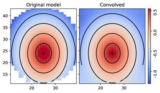
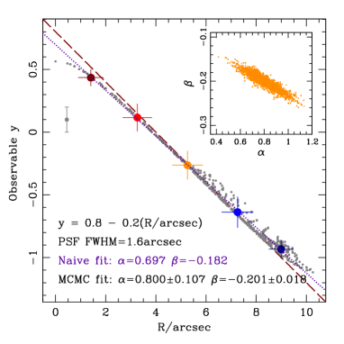
Fig. 2 illustrates the spatial resolution limit of our sample, where the effective radius, the last radial bin available from the IFU data, and the (HWHM) extent of the PSF, are compared. In most cases, the PSF width is significant, although it does not represent a major drawback: the median value of R_LAST/PSF_HWHM is 6.2, whereas the median of R_e/PSF_HWHM is 2.5. Nevertheless, we need to account for the spatial resolution limit in order to extract robust gradients, with meaningful error bars. We apply a forward modelling methodology as follows. Let us assume that $\{y_{i}\}$ represents a set of population parameters, derived from the analysis presented in §3. These observations correspond to the individual radial bins $\{R_{i}\}$. We fit the results to a model given by a linear function $y=\alpha+\beta R$, and populate the individual spaxels of the observation with this (exact) model. The model is convolved with the PSF of that observation, defined by a Moffat profile, with parameters taken from the FITS header of each observation (measured from the observation of a nearby star during the same exposures). The convolved model is then mapped on to the layout of the radial bins, in order to create a set of binned parameters $\{y^{M}_{i}\}$, that are compared with the original observations, following a standard likelihood based on a $\chi^{2}$ statistic:

$$\ln{\cal L}=\ln{\cal N}-\frac{\chi^{2}}{2},$$ (4)

where we follow the standard definition:

$$\chi^{2}=\sum_{i}\left(\frac{y_{i}-y^{M}_{i}}{\sigma_{i}}\right)^{2},$$ (5)

and $\sigma_{i}$ is the uncertainty corresponding to the derivation of the population parameter $y_{i}$. This process is implemented with an off-the-shelf MCMC sampler (emcee, Foreman-Mackey et al., 2013), to retrieve the best fit values of the slope ($\beta$) and intercept ($\alpha$), along with their uncertainties. This method is illustrated in Fig. 3 for one of the galaxies in our sample (ID 23623), whose data provide five radial apertures, and the effective radius extends over $\sim$10 times the HWHM of the PSF. The panels on the left show a test model ($y=0.8-0.2R$, where $R$ is the circularised radius of each annulus in arcsec) both before and after convolution. The radial bins are overlaid, for reference. The panel on the right shows the derivation of this test case. The grey dots are the individual (i.e. spaxel) observations, and the coloured dots are the radially binned measurements, including error bars that represent the scatter within each annulus. The dotted line traces a naive least squares fit not taking into account the effect of the PSF. It gives a slightly shallower gradient ($\beta=-0.182$), as expected, since the PSF tends to wash out any potential gradient. The method presented here gives an unbiased gradient ($\beta=-0.201\pm 0.018$), and the inset shows the potential covariance between slope and intercept. We note that this mock observation is created with comparable uncertainties to the actual observations.

5 Results

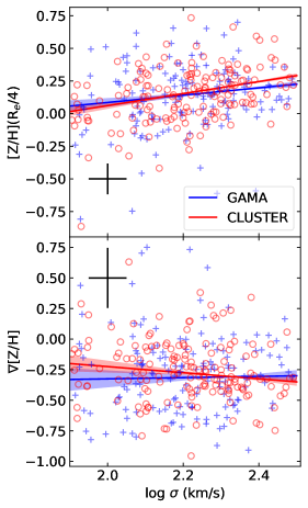
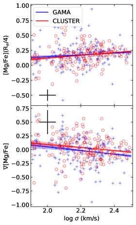
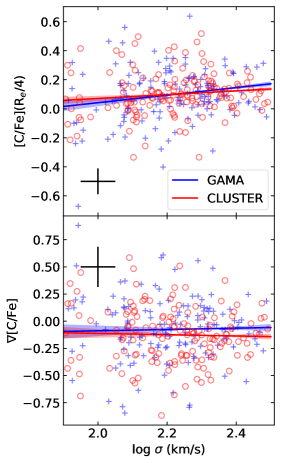
Fig. 4 shows the distribution of gradients in chemical composition with respect to velocity dispersion, from left to right, total metallicity ([Z/H]), [Mg/Fe], and [C/Fe]. GAMA ETGs are represented by blue ‘+’ symbols, and cluster galaxies appear as red ‘o’ symbols, respectively. The top panels show the value of the best linear fit at one quarter of the effective radius (R_e/4), and the bottom panels give the radial gradient, measured with respect to $\log$ R, e.g. $\nabla$[Z/H]$\equiv$d[Z/H]/d$\log$ R. A typical error bar for the individual measurements is shown in each panel. The best fit appears as a blue (red) line for GAMA (cluster) galaxies, including a shaded region that spans the 1 $\sigma$ uncertainty in the slope of the fits (the uncertainty in the intercept of these fits, defined as the value of the fit at $\sigma$=200 km s^-1, is substantially smaller than that of the slope). The top panels of the figure show the characteristic increase of metallicity and abundance ratios with respect to velocity dispersion (e.g. Trager et al., 2000).

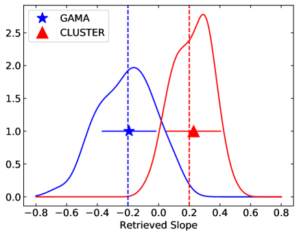
The accuracy of the method is tested on simulated data, by performing a set of 100 Monte Carlo realizations that enforce a correlation $[Z/H]=c\log\sigma_{200}$, with $c_{G}=-0.2$ for the GAMA set and $c_{C}=+0.2$ for the cluster set. Each realization features the same number of galaxies as the original set, with slopes retrieved from a Gaussian probability distribution with mean $c_{G}$ or $c_{C}$, and standard deviation corresponding to the uncertainties of the observed data. In this way, we make sure the simulated data has the same distribution of uncertainties as the original sample. Figure 5 shows the distribution of values for the whole set of 100 realizations, with the mean and standard deviation given by the symbols and error bars. The input slopes ($c_{G}$ and $c_{C}$) are represented by the vertical dashed lines, and the distribution of measured gradients shows that our method is fully consistent. Moreover, we compared the individual estimates of the slope uncertainty, produced for each realization, with the width of the distribution of slope measurements, and obtained fully consistent results: the GAMA set gave a median slope of $-0.183\pm 0.178$ whereas the median of the individual uncertainties was $0.175$; the cluster sample gave a median slope of $+0.218\pm 0.178$ and a median uncertainty of $0.155$ (all results quoted at the 1 $\sigma$ confidence level).

Figure 7: Exploring the potential drivers of population gradients for the trend of the radial gradient ($\nabla X\equiv\Delta X/\Delta\log R$).

5.1 Possible drivers of the observed trends

The observed radial gradients of the stellar populations encode the underlying formation process, including in-situ and ex-situ growth. Such a complex and entangled mixture of possible contributors can only be explored in a meaningful way if we scrutinise a reduced number of indicators we define here as “drivers” of the observed trends.

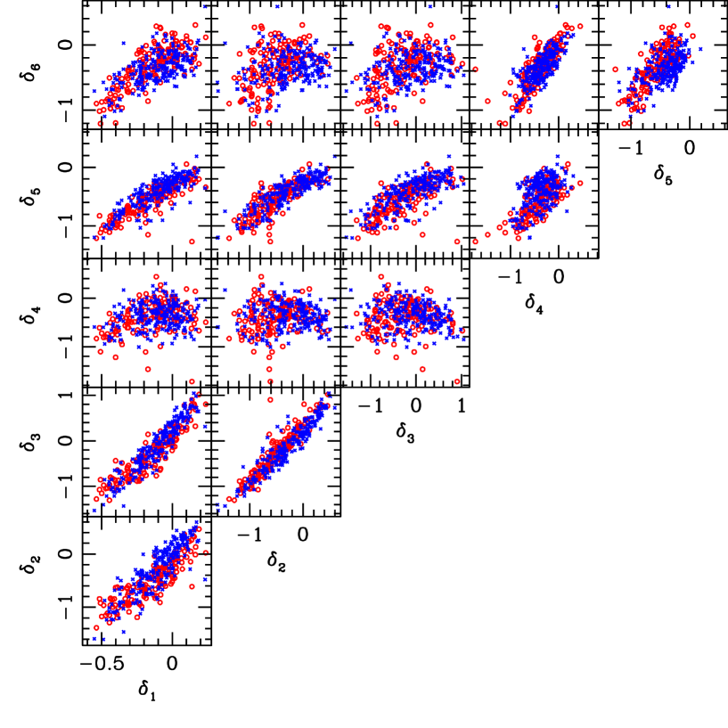
The first two columns of Table 1 define the set of six drivers adopted in this work. Our criterion for this choice is to identify observables that are relatively easy to measure from the photometric and spectroscopic properties of the sample. Motivated by the recent work on SAMI data and elsewhere (Barone et al., 2018; D’Eugenio et al., 2018), we choose the velocity dispersion (measured as averaged within an effective radius); the stellar mass; the dynamical mass; the average surface mass density (defined as $\log\Sigma_{M}=\log M_{s}-2\log$R_e); and the average gravitational potential when considering only the stellar mass (again simply defined as $\log\Phi=\log M_{s}-\log R$, i.e. disregarding dark matter and assuming a homologous distribution of matter). Note that the full gravitational potential – i.e. involving the total mass – is $\Phi\propto\sigma^{2}$, so that our first driver (velocity dispersion) can be considered a proxy of the total potential Fig. 6 compares the distribution of these drivers among one another, following the same notation as in Fig. 1. Note the strong correlation among several pairs of drivers, such as $\delta_{2}$ (stellar mass) and $\delta_{3}$ (dynamical mass), noting that these two masses are derived from independent observables. In addition to the five drivers described above, we add a new one, $\delta_{6}$, defined as $\sigma^{2}/$R_e. If we assume fully virialised systems, this driver maps the total surface mass density, and, as expected, $\delta_{6}$ correlates well with the surface stellar mass density ($\delta_{4}$).

Table A1 (in the Appendix) quantifies the slope, intercept and linear correlation coefficient of all the fits to the data, including the full set of ETGs, as well as the subsamples segregated with respect to environment (see Section 5.2 for further details about the homogenisation process applied, to minimise a bias in this regard). The error bars are quoted at the 1 $\sigma$ level. We note that there are two types of variations studied here: the radial gradient of a given observable for an individual galaxy (i.e. each of the data points in the bottom panels of Fig. 4) and the correlation of the best fit values with respect to a “driver”, such as the velocity dispersion (i.e. the slopes of the lines in Fig. 4). To avoid confusion, we refer to the former as “gradient”, and the latter as “slope”.

5.2 Homogenising the samples

In addition to the general analysis concerning trends of population gradients with respect to a number of possible physical drivers, as presented above, we also look for differences regarding environment, by comparing the GAMA sample – that represents a general field sample – and the cluster sample specifically targeted in the SAMI survey. However, differences in the distribution of the parameter under study, say velocity dispersion, between the cluster and the field sample could create a spurious difference that would be wrongly identified as an environment-related effect. To avoid this issue, we need to produce “homogeneous” subsets of GAMA and cluster galaxies that enforce the same distribution of the parameter being considered. This approach improves over a mass-function weighted analysis – implemented in, e.g., Barone et al. (2018) – by specifically constructing samples which, as far as the chosen driver is concerned, are undistinguishable. Firstly we define the target distribution as the one corresponding to the total sample with respect to the chosen driver, say velocity dispersion. Then, for either subsample (cluster or GAMA), we randomly select galaxies within a relatively narrow interval of this driver, enforcing this subsample to have the same distribution as the target one. Of course, the drawback of this method is that a number of galaxies have to be removed from the analysis to make sure the “shape of the histogram” is the same in both subsets. However, no significant variations are found in different realizations.

Figure 8: Exploring a number of possible drivers of population gradients for the trend of the “central” values (corresponding to the linear fit estimated at R_e/4).

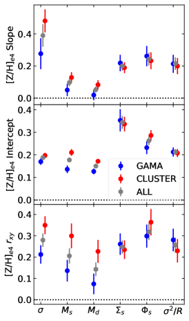
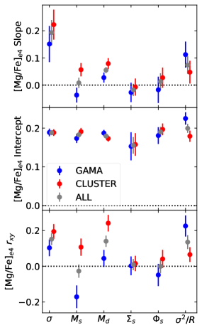
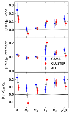
Table 1 shows the statistical differences measured between the original sample and the homogenised one. For each driver, we give the final number of galaxies in each subsample (being equal, by construction), the KS statistic ($D_{KS}$) for the original and homogeneous samples, and the KS statistic corresponding to a fully random set: this one is obtained by randomly reshuffling the targeted samples 1,000 times, producing a distribution of D_KS from which the mean and standard deviation are quoted.

The results of the slopes and intercepts for the whole set of six drivers are show on Tables A1 and A2. A linear regression is applied both to the radial gradients, and the central values of the parameters. The models for stellar parameter $\pi$ are thus $\nabla\pi=a\delta+b$ (for the gradient) and $[\pi]_{\rm e4}=a\delta+b$ (for the central value), where $\delta$ is one of the six drivers defined above, and $\pi$ corresponds to either total metallicity ([Z/H]), [Mg/Fe], [C/Fe] or (log) stellar age. $r_{xy}$ is the linear correlation coefficient. The error bars, quoted at the 1 $\sigma$ level, take into account the individual uncertainties of the measurements. The intercepts are given by the $b$ coefficients, and correspond to the population parameter at a reference value of the driver, as shown in col. 2 of Table 1. These reference values adopt a fiducial galaxy with velocity dispersion $\sigma$=200 km s^-1, stellar (or dynamical) mass M${}_{s}=1\times 10^{11}$M_⊙, and effective radius R_e=2 kpc.

6 Discussion

We split the discussion into a general analysis of the trends with respect to the drivers defined above (Table 1), followed by a comparison of the results with respect to environment, i.e. contrasting the GAMA and cluster subsamples.

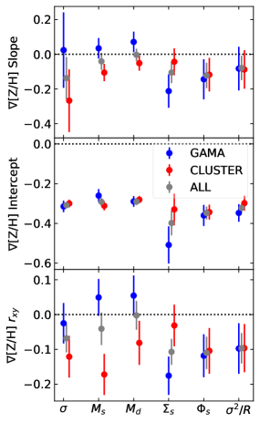
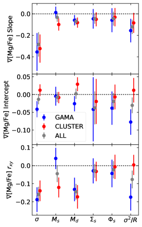
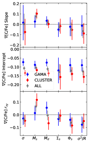
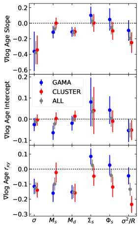
The results obtained with respect to the different drivers are shown in Figs. 7, 8 and 9, and quantified in Tables A1 and A2. The information for each observable is presented in three vertical panels: the top one gives the slope of the (linear) trend corresponding to the chosen observable with respect to the driver labelled in the horizontal axis; the middle panel is the intercept of this linear trend, estimated at the reference value of the driver (as shown on col. 2 of Table 1), and the bottom panel is the linear correlation coefficient. All data points include error bars at the 1 $\sigma$ level. We should emphasize that the measurements at fixed, say, velocity dispersion typically vary less than the trends with respect to the driving parameter. As expected, the correlation coefficients of the trends involving the intercepts are higher than those for the gradients, as this measurement is less noisy.

6.1 General trends

In this part of the discussion, we focus on the general trend, shown by the grey data points. Of the six drivers, velocity dispersion ($\sigma$) appears to be the dominant one, with strongly correlated trends in all observables, except, perhaps, $\nabla$[C/Fe]. This result is consistent with the analysis of Barone et al. (2018), who concluded that $g-i$ colour and total stellar metallicity correlate stronger with the gravitational potential ($\Phi\propto\sigma^{2}$) than with mass. This result is also in agreement with previous work based on a larger sample of ETGs (see, e.g. Bernardi et al., 2003), and with independent studies of samples extracted from the same dataset (Scott et al., 2017; Barone et al., 2018). In the following discussion, we will focus on this driver, with occasional reference to the others.

[Z/H], as measured at R_e/4 ([Z/H]_e4), increases strongly with $\sigma$. The radial gradients are overall substantially negative, featuring a weak, negative trend with respect to $\sigma$. At the fiducial value of velocity dispersion ($\sigma$=200 km s^-1), the total metallicity is unsurprisingly super-solar ([Z/H]=$+0.19\pm 0.01$) with a strong negative gradient ($\nabla$[Z/H]=$-0.31\pm 0.02$). The slope of [Z/H]_e4 is positive in all six drivers, although they are significant, in addition to $\sigma$, with stellar mass surface density, stellar potential and $\sigma^{2}/R$. We note that the slope of the metalliticy-velocity dispersion trend lies between $+0.46$ and $+0.28$ (see Table A1), values that are comparably shallower than previous estimates, such as $+0.58\pm 0.05$ (La Barbera et al., 2014) and $+0.65\pm 0.02$ (Thomas et al., 2010). However, we should note that this work gives the metallicity at R_e/4, whereas the quoted values correspond to an average metallicity within the central regions of the galaxy. Also, as shown in Harrison et al. (2011, see their table 5), different studies find a wide range of this slope, from $\sim+$0.18 to $\sim+$0.79. These variations are likely caused by different methods to derive the stellar population parameters, as well as different selection criteria. Our values of the metallicity-$\sigma$ slope fall within the range reported by Harrison et al. (2011)

Figure 9: Equivalent version of Figs. 7 (left, radial gradient trends) and 8 (right, central value trends), regarding (log) stellar ages.

[Mg/Fe] features a strong positive slope regarding the central value (i.e. higher [Mg/Fe]_e4 with increasing $\sigma$), a well-known correlation typically explained as a shorter duration of star formation in more massive galaxies (see, e.g. Trager et al., 2000; Thomas et al., 2005; de La Rosa et al., 2011), as expected from the delayed contribution of Fe-rich yields from type Ia supernovae with respect to the $\alpha$-rich ejecta from type II. In addition, we find a strong negative trend in the slope of $\nabla$[Mg/Fe] (i.e. more strongly decreasing [Mg/Fe] outwards in more massive galaxies). This trend is suggestive of a more complex ex-situ formation scenario, where the stellar component in the outer regions is populated by later stages of star formation with higher chemical processing, therefore with a lower [Mg/Fe]. The different slope in the trends of [Mg/Fe]_e4 and $\nabla$[Mg/Fe] pose a significant caveat in the analysis, regarding the radial position at which [Mg/Fe] is estimated. As we progress towards more massive galaxies, the higher central [Mg/Fe] is compensated by a more negative gradient, so that estimates of the [Mg/Fe] vs $\sigma$ slope will differ greatly when evaluated at, say R_e/4 or 2R_e. Indeed, Greene et al. (2015) found that, while in the galaxy centre [Mg/Fe] increases with $\sigma$, this positive correlation disappears as one moves towards larger galactocentric radii. Parikh et al. (2019) analysed abundance pattern gradients as a function of galaxy mass in a sample of SDSS/MaNGA galaxies. As shown in their fig. 3, the positive correlation of [Mg/Fe] with mass in the galaxy centre tends to disappear towards larger radii (beyond $\sim$R_e/2), a qualitatively consistent result with Greene et al. (2015) and our work.

At the fiducial value of $\sigma$, the central value is markedly super-solar ([Mg/Fe]_e4=$+0.19\pm 0.01$ dex) with a rather shallow gradient ($\nabla$[Mg/Fe]=$-0.01\pm 0.01$). Note the slope of [Mg/Fe] – both the radial gradient and the central value – do not correlate strongly with any of the other drivers, giving more support to the idea that velocity dispersion, or equivalently, the gravitational potential, is the major driver of the stellar population content in ETGs.

[C/Fe], evaluated at R_e/4, shows a rather large amount of scatter, but, again, $\sigma$ is the stronger driver, with a significant increasing trend of the central value. This result agrees with previous work (Kelson et al., 2006; Graves et al., 2007; Schiavon, 2007; Smith et al., 2009; Johansson, Thomas, & Maraston, 2012). The slope of $\nabla$[C/Fe] is consistent with zero, in contrast with the strong negative slope of $\nabla$[Mg/Fe] with respect to $\sigma$. The trends in [C/Fe] roughly parallel those found for [Z/H]. At the fiducial value of velocity dispersion, [C/Fe] is super-solar ([C/Fe]_e4=$+0.11\pm 0.01$) with a negative radial gradient ($\nabla$[C/Fe]=$-0.10\pm 0.01$), once more a signature of a substantially different population in the outer envelope.

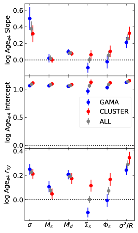
Stellar age is also driven by velocity dispersion, with $\delta_{6}\equiv\sigma^{2}/R$ becoming an equally strong driver, especially if we consider that the correlation coefficient is higher in $\delta_{6}$ (with respect to $\delta_{1}$) for the age at R_e4, and also for the radial gradient of the age in the cluster subsample. Moreover, note the slope of the total gravitational potential is 1/2 of the slope with respect to $\sigma$. The trend shows an increasing age with $\sigma$ as well as a decreasing radial gradient with $\sigma$, although we note that at the fiducial value, this gradient is compatible with zero ($\nabla\log$Age=$-0.02\pm 0.02$). Given that most of our ETGs lie below the fiducial value of $\sigma$, we conclude that at the low mass end of the sample, the radial gradient of age is positive, i.e. harbouring older populations in the outer regions.

6.2 Environment-related trends

We now turn our attention to differences in the observed trends between cluster and field/group ETGs. Figs. 7 and 8 plot these two data sets independently, with cluster ETGs shown in red and GAMA ETGs shown in blue. Tables A1 and A2 also quantify the trends separately for each subsample.

It is quite remarkable to find relatively weak variations between a cluster and a field/group environment. The stark contrast between velocity dispersion and environment as drivers of the underlying stellar populations has already been presented in previous work (see, e.g. Rogers et al., 2010; Thomas et al., 2010; La Barbera et al., 2014; Greene et al., 2015; Rosani et al., 2018). In our data, most of the differences stay within the 1-2 $\sigma$ level, and need to rely on the linear correlation coefficient to confirm these variations. The most conspicuous one is the slope of [Z/H]_e4 with respect to velocity dispersion, with a steeper slope in a cluster environment. This result would suggest that ETGs at the massive end are more metal-rich in a cluster environment, a result that could be explained by a higher chemical processing expected in a system with more efficient star formation. This trend is followed, although weakly, by [Mg/Fe]_e4 but it is intriguingly reversed in the case of [C/Fe]_e4.

Although the metallicity gradient, $\nabla$[Z/H], is similar in both types of environment, cluster ETGs show a strong negative change of this gradient with increasing velocity dispersion, whereas the field sample shows no measurable trend. This behaviour is consistent with a scenario where field ETGs accrete more inhomogeneous material through mergers, a possible sign of galactic conformity (Weinmann et al., 2006), whereby the stellar populations of galaxies within a group correlate with those of the central galaxy. In a cluster environment, we therefore expect that the properties of the merging progenitors were more homogeneous with respect to their field counterparts. The trends with [C/Fe] are similar to [Mg/Fe]. Note that the correlation coefficient of the $\nabla$[Z/H] trends (bottom-left panel of Fig. 7) is more prominent in the cluster sample, perhaps reflecting a more uniform star formation (and merger) history.

It is also worth mentioning the fiducial value of $\nabla$[Mg/Fe] (at $\sigma$=200 km s^-1), with a sizeable difference between cluster and GAMA ETGs, the latter having a slightly negative radial gradient. The fiducial $\nabla$[C/Fe] shows the opposite trend, with cluster ETGs having a steeper, more negative radial gradient. In contrast, the fiducial $\nabla$[Z/H] is the same in both subsamples.

Interestingly, by looking at the correlation coefficients, we note that the other drivers sometimes feature stronger environment-related differences. Such is especially the case with stellar mass. As regards to age (i.e. differences in the time evolution of star formation histories), no difference is found with respect to environment. Only the mass surface density (both stellar and $\sigma^{2}/R$) appear to show a difference in the central value of age, with older ages in cluster environments. This result aligns with the proposal of Barone et al. (2018) of a correlation between age and stellar mass density.

7 Summary

We study the radial gradients of early-type galaxies (ETGs) by use of integral field unit data from the SAMI survey. Our working sample comprises 522 visually classified ETGs located in the GAMA survey (that maps field and group environments) as well as cluster galaxies. This unique sample definition makes SAMI an ideal dataset to explore environment-related mechanisms. In this case we focus on the stellar population content, fitting radial gradients of total metallicity, [Mg/Fe], [C/Fe] as well as stellar age. A set of six possible drivers are adopted (Table 1, and Fig. 6), and two main issues are sought: 1) to identify the dominant driver of the radial gradients, and quantify the trends, and 2) to determine the role of field/cluster environment in the formation process of ETGs.

Our results (condensed in Figs. 7, 8, and 9; and quantified in Tables A1, and A2) include a large amount of information that should be used as constraints on numerical models of galaxy formation. An incomplete, concise list of results follows:

$\bullet$ The dominant driver controlling the stellar population properties of ETGs is velocity dispersion ($\sigma$). Our work extends similar past claims by looking in detail at a set of six different physical estimates as possible drivers, finding that $\sigma$ is the one with strongly correlated trends regarding radial gradients and central values of the stellar population properties. We note that $\sigma$ is formally equivalent to the total gravitational potential ($\Phi\propto\sigma^{2}$), albeit with slopes differing by a factor of 1/2.

$\bullet$ Surface mass density (regarding both total, $\delta_{6}$, and stellar, $\delta_{4}$), also produces substantially strong correlations, especially with respect to the radial gradient of stellar age.

$\bullet$ Focusing on velocity dispersion (or gravitational potential) as the main driver, we find a strong negative gradient of total metallicity ($\nabla$[Z/H]) with a weak dependence with respect to $\sigma$. [C/Fe] appears to behave similarly to total metallicity but the correlation is weaker. In contrast, the dependence of $\nabla$[Mg/Fe] on $\sigma$ is quite steep and negative, so that the gradient is rather flat at the massive end of this sample, turning to a strongly positive slope at the low mass end. These trends suggest the merging progenitors that contributed to populate the outer envelope of massive ETGs during the ‘second stage’ cannot be equivalent to low mass galaxies at present. As regards to the central values (measured at R_e/4), we find, unsurprisingly, substantial, positive slopes in all population indicators, meaning that massive ETGs are older, more metal rich, and with higher abundance ratios, a well-known result (see, e.g., Renzini, 2006).

$\bullet$ Environment-related differences are subdominant, confirming previous work in the literature. Our results quantify in detail the variations in population gradients between a field/group and a cluster environment, finding that in the central regions of galaxies (evaluating the trends at R_e/4), cluster galaxies have more positively increasing slopes of [Z/H] and [Mg/Fe] with $\sigma$, i.e. massive galaxies with the strongest gravitational potential are more metal rich and [Mg/Fe] overabundant in a cluster environment, with respect to the field. This trend intriguingly reverses for [C/Fe], although the amount of scatter is rather high. Environment-related differences in the trends regarding radial gradients are harder to measure, but there is some evidence that cluster ETGs have steeper (negative) slopes of the trend between $\nabla$[Z/H] and $\sigma$ but no measurable difference in $\nabla$[Mg/Fe]. In contrast, the value of $\nabla$[Mg/Fe] at fixed velocity dispersion appears shallower in cluster galaxies.

References

- Bacon et al. (2001) Bacon R., et al., 2001, MNRAS, 326, 23
- Barone et al. (2018) Barone, T. M., et al., 2018, ApJ, 856, 64
- Bernardi et al. (2003) Bernardi M., et al., 2003, AJ, 125, 1882
- Bland-Hawthorn et al. (2011) Bland-Hawthorn, J., et al., 2011, Optics Express, 19, 2649
- Boardman et al. (2017) Boardman N. F., et al., 2017, MNRAS, 471, 4005
- Bryant et al. (2014) Bryant, J. J., Bland-Hawthorn, J., Fogarty, L. M. R., Lawrence, J. S., Croom, S. M., 2014, MNRAS, 438, 869
- Bryant et al. (2015) Bryant J. J., et al., 2015, MNRAS, 447, 2857
- Bundy et al. (2015) Bundy K., et al., 2015, ApJ, 798, 7
- Cappellari & Emsellem (2004) Cappellari, M., Emsellem, E., 2004, PASP, 116, 138
- Cappellari et al. (2011) Cappellari M., et al., 2011, MNRAS, 413, 813
- Cervantes & Vazdekis (2009) Cervantes, J. L., Vazdekis, A., 2009, MNRAS, 392, 691
- Chabrier (2003) Chabrier, G., 2003, PASP, 115, 763
- Conroy & van Dokkum (2012) Conroy, C., van Dokkum, P., 2012, ApJ, 747, 69
- Cook et al. (2016) Cook B. A., Conroy C., Pillepich A., Rodriguez-Gomez V., Hernquist L., 2016, ApJ, 833, 158
- Cortese et al. (2016) Cortese, L., et al., 2016, MNRAS, 463, 170
- Croom et al. (2012) Croom S. M., et al., 2012, MNRAS, 421, 872
- Daddi et al. (2005) Daddi E., et al., 2005, ApJ, 626, 680
- de La Rosa et al. (2011) de La Rosa I. G., La Barbera F., Ferreras I., de Carvalho R. R., 2011, MNRAS, 418, L74
- D’Eugenio et al. (2018) D’Eugenio F., Colless M., Groves B., Bian F., Barone T. M., 2018, MNRAS, 479, 1807
- Driver et al. (2011) Driver S. P., et al., 2011, MNRAS, 413, 971
- Foreman-Mackey et al. (2013) Foreman-Mackey D., Hogg D. W., Lang D., Goodman J., 2013, PASP, 125, 306
- Goddard et al. (2017) Goddard D., et al., 2017, MNRAS, 465, 688
- González-Delgado et al. (2015) González-Delgado, R., et al., 2015, A&A, 581, A103
- Graves et al. (2007) Graves G. J., Faber S. M., Schiavon R. P., Yan R., 2007, ApJ, 671, 243
- Greene et al. (2015) Greene J. E., Janish R., Ma C.-P., McConnell N. J., Blakeslee J. P., Thomas J., Murphy J. D., 2015, ApJ, 807, 11
- Harrison et al. (2011) Harrison C. D., Colless M., Kuntschner H., Couch W. J., de Propris R., Pracy M. B., 2011, MNRAS, 413, 1036
- Hirschmann et al. (2015) Hirschmann M., Naab T., Ostriker J. P., Forbes D. A., Duc P.-A., Davé R., Oser L., Karabal E., 2015, MNRAS, 449, 528
- Johansson, Thomas, & Maraston (2012) Johansson J., Thomas D., Maraston C., 2012, MNRAS, 421, 1908
- Kelson et al. (2006) Kelson D. D., Illingworth G. D., Franx M., van Dokkum P. G., 2006, ApJ, 653, 159
- Kelvin et al. (2012) Kelvin, L. S., et al. 2012, MNRAS, 421, 1007
- La Barbera et al. (2011) La Barbera F., Ferreras I., de Carvalho R. R., Lopes P. A. A., Pasquali A., de la Rosa I. G., De Lucia G., 2011, ApJ, 740, L41
- La Barbera et al. (2013) La Barbera, F., Ferreras, I., Vazdekis, A., de la Rosa, I. G., de Carvalho, R. R., Trevisan, M., Falcón-Barroso, J., Ricciardelli, E., 2013, MNRAS, 433, 3017 (LB13)
- La Barbera et al. (2014) La Barbera F., Pasquali A., Ferreras I., Gallazzi A., de Carvalho R. R., de la Rosa I. G., 2014, MNRAS, 445, 1977
- La Barbera et al. (2016) La Barbera F., Vazdekis A., Ferreras I., Pasquali A., Cappellari M., Martín-Navarro I., Schönebeck F., Falcón-Barroso J., 2016, MNRAS, 457, 1468
- Lackner et al. (2012) Lackner C. N., Cen R., Ostriker J. P., Joung M. R., 2012, MNRAS, 425, 641
- Larson (1974) Larson, R. B., 1974, MNRAS, 166, 585
- Martín-Navarro et al. (2018) Martín-Navarro I., Vazdekis A., Falcón-Barroso J., La Barbera F., Yıldırım A., van de Ven G., 2018, MNRAS, 475, 3700
- Oser et al. (2010) Oser L., Ostriker J. P., Naab T., Johansson P. H., Burkert A., 2010, ApJ, 725, 2312
- Owers et al. (2017) Owers M. S., et al., 2017, MNRAS, 468, 1824
- Owers et al. (2018) Owers M. S., et al., 2019, ApJ, 873, 52
- Parikh et al. (2019) Parikh T., et al., 2019, MNRAS, 483, 3420
- Peng et al. (2010) Peng Y.-j., et al., 2010, ApJ, 721, 193
- Renzini (2006) Renzini A., 2006, ARA&A, 44, 141
- Rogers et al. (2010) Rogers B., Ferreras I., Pasquali A., Bernardi M., Lahav O., Kaviraj S., 2010, MNRAS, 405, 329
- Rosani et al. (2018) Rosani G., Pasquali A., La Barbera F., Ferreras I., Vazdekis A., 2018, MNRAS, 476, 5233
- Sánchez-Blázquez et al. (2014) Sánchez-Blázquez P., et al., 2014, A&A, 570, A6
- Sánchez et al. (2012) Sánchez S. F., et al., 2012, A&A, 538, A8
- Schiavon (2007) Schiavon R. P., 2007, ApJS, 171, 146
- Scott et al. (2017) Scott N., et al., 2017, MNRAS, 472, 2833
- Scott et al. (2018) Scott N., et al., 2018, MNRAS, 481, 2299
- Smith et al. (2009) Smith R. J., Lucey J. R., Hudson M. J., Bridges T. J., 2009, MNRAS, 398, 119
- Smith et al. (2012) Smith R. J., Lucey J. R., Price J., Hudson M. J., Phillipps S., 2012, MNRAS, 419, 3167
- Thomas et al. (2005) Thomas D., Maraston C., Bender R., Mendes de Oliveira C., 2005, ApJ, 621, 673
- Thomas et al. (2010) Thomas D., Maraston C., Schawinski K., Sarzi M., Silk J., 2010, MNRAS, 404, 1775
- Thomas, Maraston & Johansson (2011) Thomas, D., Maraston, C., Johansson, J., 2011, MNRAS, 412, 2183
- Trager et al. (1998) Trager, S. C., Worthey, G., Faber, S. M., Burstein, D., González, J. J., 1998, ApJS, 116, 1
- Trager et al. (2000) Trager, S. C., et al. 2000, AJ, 120, 165
- Trujillo et al. (2006) Trujillo I., et al., 2006, ApJ, 650, 18
- van de Sande et al. (2017) van de Sande J., et al., 2017, ApJ, 835, 104
- van Dokkum et al. (2008) van Dokkum P. G., et al., 2008, ApJ, 677, L5
- Vazdekis et al. (2015) Vazdekis, A., Coelho, P., Cassisi, S., Ricciardelli, E., Falcón-Barroso, J., Sánchez-Blázquez, P., La Barbera, F., Beasley, M. A., Pietrinferni, A., 2015, MNRAS, 449, 1177
- Weinmann et al. (2006) Weinmann S. M., van den Bosch F. C., Yang X., Mo H. J., 2006, MNRAS, 366, 2