Dynamical signatures of quantum chaos and relaxation timescales in a spin-boson system

Abstract

Quantum systems whose classical counterparts are chaotic typically have highly correlated eigenvalues and level statistics that coincide with those from ensembles of full random matrices. A dynamical manifestation of these correlations comes in the form of the so-called correlation hole, which is a dip below the saturation point of the survival probability’s time evolution. In this work, we study the correlation hole in the spin-boson (Dicke) model, which presents a chaotic regime and can be realized in experiments with ultracold atoms and ion traps. We derive an analytical expression that describes the entire evolution of the survival probability and allows us to determine the timescales of its relaxation to equilibrium. This expression shows remarkable agreement with our numerical results. While the initial decay and the time to reach the minimum of the correlation hole depend on the initial state, the dynamics beyond the hole up to equilibration is universal. We find that the relaxation time of the survival probability for the Dicke model increases linearly with system size.

I Introduction

The subject of equilibration and thermalization of isolated quantum systems in the chaotic regime has seen a great deal of advance in the last years Reimann (2008); Short (2011); Short and Farrelly (2012); Zangara et al. (2013); He et al. (2013); Gogolin and Eisert (2016); Borgonovi et al. (2016); Alessio et al. (2016); Dymarsky (a); Reimann (2018a); *Reimann2018b. Equilibration is reached when, after a transient time, the observable under investigation shows only small fluctuations around an asymptotic value, and these fluctuations decrease with system size. Thermalization implies that this infinite-time average is very close to the predictions from statistical mechanics, and the difference between the two also decreases with system size. In this picture, an important open question is how long it takes for isolated quantum systems to reach equilibrium. Despite the increasing number of recent works addressing this issue Monnai (2013); Goldstein et al. (2013); Malabarba et al. (2014); Goldstein et al. (2015); Gogolin and Eisert (2016); Reimann (2016); García-Pintos et al. (2017); de Oliveira et al. (2018); Dymarsky (b); Chan et al. (2018); Bertini et al. (2018); Schiulaz et al. ; Borgonovi et al. (2019), there is no agreement regarding how the relaxation timescale should depend on system size, range of interactions, observables, and initial states.

The last steps of the evolution toward equilibrium, after the dynamics resolves the discreteness of the spectrum, are determined by the properties of the eigenvalues Schiulaz et al. . The largest possible timescale is the Heisenberg time Berry (1983), which is proportional to the inverse of the mean level spacing of the region of the spectrum probed by the initial state. Before reaching this timescale, effects of the correlations between the eigenvalues may be observed. In the case of the survival probability footSurv , which is the probability of finding the initial state at time $t$, these correlations cause a decay below the saturation value of the dynamics, known as correlation hole footNote . This phenomenon was first studied in the context of molecules, where the interest was not exactly in dynamics, but in alternative ways to detect level repulsion in systems without good line resolution Leviandier et al. (1986); Guhr and Weidenmüller (1990); Wilkie and Brumer (1991).

The correlation hole has been studied in full random matrices Alhassid and Levine (1992), in many-body systems with Torres-Herrera and Santos (2017a, b); Torres-Herrera et al. (2018); Torres-Herrera and Santos (2019); Schiulaz et al. and without disorder Torres-Herrera and Santos (2017b), in the Sachdev-Ye-Kitaev model Cotler et al. (2017); Gharibyan et al. (2018); Nosaka et al. (2018), which is a two-body random ensemble Brody et al. (1981), and in the finite one-dimensional Anderson model TorresARXIV . The hole is not exclusive to the survival probability, but emerges also in experimental local observables Torres-Herrera et al. (2018); Torres-Herrera and Santos (2019). For the correlation hole to be visible, one needs to perform large averages over initial states and, in the case of Hamiltonian matrices with random elements, over ensembles of Hamiltonian realizations. In Ref. Schiulaz et al. , it was shown that in realistic chaotic many-body quantum systems with local short-range interactions and perturbed far from equilibrium, the time to reach the minimum of the correlation hole increases exponentially with system size. This timescale, which is still shorter than the Heisenberg time, was referred to as Thouless time due to its relationship with the Thouless energy computed from random matrix theory. As explained in Schiulaz et al. , the Thouless time in interacting systems is the time that it takes for an initial state to spread over the entire Hilbert space accessible to its energy. Beyond this point, the dynamics becomes universal all the way to equilibrium.

In the present work, we use the survival probability to study the correlation hole in the Dicke model. This is a paradigmatic spin-boson model with two degrees of freedom. It has a classical counterpart and exhibits chaos for several values of its parameters, mostly for high excitation energies and in the superradiant phase. The model was first introduced to explain superradiance Dicke (1954); Garraway (2011); Baumann et al. (2010, 2011) and has since then been used in different contexts, from quantum chaos Lewenkopf et al. (1991); Emary and Brandes (2003a); *Emary2003; Bastarrachea-Magnani et al. (2014a); *Bastarrachea2015; *Bastarrachea2016PRE; Chávez-Carlos et al. (2016) and quantum batteries Andolina et al. to excited-state quantum phase transitions Pérez-Fernández et al. (2011a); Brandes (2013); Bastarrachea-Magnani et al. (2014b); Larson and Irish (2017) and quench dynamics Pérez-Fernández et al. (2011b); Altland and Haake (2012); Lerma-Hernández et al. (2018); Kloc et al. (2018). Recently, the model was employed in a study of the out-of-time ordered correlator (OTOC), where it was shown that, in the chaotic regime, the OTOC increases exponentially in time with a rate comparable to the classical Lyapunov exponent Chávez-Carlos et al. (2019). In addition to ultracold atoms in optical cavities Baden et al. (2014); Klinder et al. (2015), the Dicke model can now be realized also with ion traps Cohn et al. (2018). The latter is one of the main platforms to study long-time coherence evolution Blatt and Roos (2012), which makes the analysis of the timescales involved in the relaxation process of the Dicke model a timely subject.

We obtain an analytical expression that describes the entire evolution of the survival probability for the Dicke model in the chaotic regime. The expression describes very accurately our numerical results, and with it, we can derive analytically the timescales involved in the relaxation process. We find that the relaxation time increases linearly with system size, while the Thouless time depends non trivially on the initial state.

The article is organized as follows. In Sec. II, we describe the Dicke model and the properties associated with its eigenvalues. In Sec. III, we discuss the initial states considered and present the analytical expression for the survival probability. This expression is compared with numerical results in Sec. IV. The analytical expressions for the Thouless and relaxation times are given and discussed in Sec. V. We present our conclusions in Sec. VI.

II Dicke Model

The Dicke model Dicke (1954) describes the interaction between a set of $\mathcal{N}$ two-level atoms with energy splitting $\omega_{0}$ and a single mode of the electromagnetic field with radiation frequency $\omega$. By setting $\hbar=1$, the time-reversal symmetric Hamiltonian of the model is written as

$$\hat{H}_{D}=\omega\hat{a}^{\dagger}\hat{a}+\omega_{0}\hat{J}_{z}+\frac{2\gamma}{\sqrt{\mathcal{N}}}\hat{J}_{x}(\hat{a}^{\dagger}+\hat{a}).$$ (1)

The first term of the equation above accounts for the energy of the field, where $\hat{a}^{\dagger}$ ($\hat{a}$) is the bosonic creation (annihilation) operator. The second term corresponds to the energy of the atoms, where $\hat{J}_{x,y,z}=\frac{1}{2}\sum_{k=1}^{\mathcal{N}}\sigma_{x,y,z}^{k}$ are the atomic pseudo-spin operators and $\sigma_{x,y,z}$ are the Pauli matrices. The third term describes the atom-field interaction with coupling parameter $\gamma$. The eigenvalues $j(j+1)$ of the operator $\hat{\textbf{J}}^{2}=\hat{J}_{x}^{2}+\hat{J}_{y}^{2}+\hat{J}_{z}^{2}$ determine different invariant subspaces. Its maximum value, given by $j=\mathcal{N}/2$, defines the symmetric non-degenerate atomic subspace that includes the ground-state. The Hamiltonian $\hat{H}_{D}$ commutes with the parity operator $\hat{\Pi}=e^{i\pi\hat{\Lambda}}$, where $\hat{\Lambda}=\hat{a}^{\dagger}\hat{a}+\hat{J}_{z}+j\hat{1}$. The operator $\hat{\Lambda}$ represents the total number of excitations with eigenvalues $\lambda=n+m+j$, where $n$ is the number of photons, $m+j$ is the number of excited atoms, and $m$ is the eigenvalue of $\hat{J}_{z}$. In all calculations presented below, we consider the positive parity spectrum of the model.

When the coupling parameter reaches a critical value $\gamma_{c}=\sqrt{\omega\omega_{0}}/2$, a second-order quantum phase transition takes place Hepp and Lieb (1973a, b). The system goes from a normal phase ($\bar{\gamma}<1$ with $\bar{\gamma}=\gamma/\gamma_{c}$), where the ground state has no photons and all the atoms are in their lowest level, to a superradiant phase ($\bar{\gamma}>1$), where the ground state has non-zero expectation values for the number of photons and number of excited atoms.

II.1 Level Statistics and Density of States

The classical limit of the Dicke model can be obtained by using Bloch and Glauber coherent states Bastarrachea-Magnani et al. (2014b, a, 2015); Chávez-Carlos et al. (2016), which allows for the identification of the parameters and energy range that lead to chaos. A main signature of classical chaos in the quantum regime is energy-level repulsion Casati1980 ; Bohigas1984 .

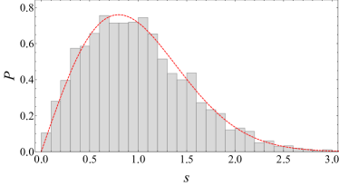
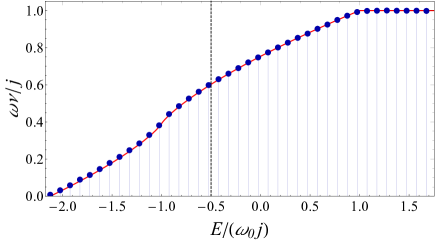
As our case study, we choose $\omega=\omega_{0}$ and $j=100$, and we select a coupling parameter in the superradiant phase, $\bar{\gamma}=2$. For these values, chaos is found at excitation energies above $E\approx-1.6\omega_{0}j$ (see Ref. Chávez-Carlos et al. (2016)). We choose an energy well above this threshold, $E_{c}=-0.5\omega_{0}j$, for which the whole energy shell is covered by chaotic trajectories (see Ref. Chávez-Carlos et al. (2016)). In Fig. 1 (a), we show the level spacing distribution, denoted by $P(s)$, where $s$ is the spacing between nearest-neighboring unfolded energy levels from an energy interval around $E_{c}$. In quantum systems whose classical counterparts are chaotic, the levels are prohibited from crossing and $P(s)$ coincides with the Wigner surmise Guhr et al. (1998), as indeed confirmed in Fig. 1 (a).

(a)

(b)

Figure 1: (Color online) In (a): The level spacing distribution for the unfolded spectrum (shaded area) in the energy region $E/(\omega_{0}j)\in[-0.8,-0.2]$ agrees with the Wigner surmise (dashed line). In (b): Density of states (DoS) evaluated numerically (blue circles) with bin size $\Delta E=0.1\omega_{0}j$ and analytical expression (2) indicated with the red solid curve. Parameters: $\omega=\omega_{0}$, $\bar{\gamma}=2$, $j=100$, and positive parity. The vertical line in (b) indicates the energy $E_{c}=-0.5\omega_{0}j$ chosen for our study. A truncated Hilbert space was employed using the basis of Refs. Bastarrachea-Magnani and Hirsch (2014); Hirsch and Bastarrachea-Magnani (2014), ensuring 24 453 converged eigenenergies, which range from the ground state energy $E_{gs}=-2.125\omega_{0}j$ until $E_{T}=1.755\omega_{0}j$.

With the classical Hamiltonian, it is possible to estimate the energy averaged density of states (DoS), which is given by the expression Bastarrachea-Magnani et al. (2014b),

$$\nu(E)=\frac{j}{\omega}\left\{\begin{array}[]{l}\frac{1}{\pi}\int_{y_{-}}^{y_{+}}dy\cos^{-1}\left(\sqrt{\frac{2(y-\epsilon)}{\bar{\gamma}^{2}(1-y^{2})}}\right),\epsilon_{gs}\leq\epsilon<-1\\ \frac{1+\epsilon}{2}+\frac{1}{\pi}\int_{\epsilon}^{y_{+}}dy\cos^{-1}\left(\sqrt{\frac{2(y-\epsilon)}{\bar{\gamma}^{2}(1-y^{2})}}\right),|\epsilon|\leq 1\\ 1,\epsilon>1\end{array}\right.$$ (2)

where $y_{\pm}=-\bar{\gamma}^{-1}\left(\bar{\gamma}^{-1}\mp\sqrt{2(\epsilon-\epsilon_{gs})}\right)$ and $\epsilon=\frac{E}{\omega_{0}j}$ is the normalized energy. The ground state energy is $\epsilon_{gs}=-1$ for the normal phase, while it is $\epsilon_{gs}=-\dfrac{1}{2}\left(\bar{\gamma}^{2}+\bar{\gamma}^{-2}\right)$ in the superradiant phase. In Fig. 1 (b), we compare the DoS obtained numerically with the expression (2). The agreement is excellent. It is evident from the figure that for $|\epsilon|\leq 1$, the DoS shows a linear dependence on energy, $\nu(E)\propto E$. Our choice of the value of $E_{c}$ for the studies below falls within this region. Notice also that the DoS in Eq. (2) scales linearly with the number of atoms ($j$ appears explicitly in the beginning of the equation), a property that will be useful below to determine the dependence of the timescales of the model on the number of atoms.

III Survival probability and Initial states

The survival probability, $S_{P}(t)$, is a dynamical observable defined as the probability to find an arbitrary initial quantum state $|\Psi(0)\rangle$ at a later time $t$,

$$S_{P}(t)=|\langle\Psi(0)|\Psi(t)\rangle|^{2}.$$ (3)

By writing the initial state in terms of the energy eigenbasis, $|\Psi(0)\rangle=\sum_{k}c_{k}|\phi_{k}\rangle$, where $\hat{H}|\phi_{k}\rangle=E_{k}|\phi_{k}\rangle$ and $c_{k}=\langle\phi_{k}|\Psi(0)\rangle$, the survival probability is

$$S_{P}(t)=\left|\sum_{k}|c_{k}|^{2}e^{-iE_{k}t}\right|^{2}.$$ (4)

The short-time evolution depends on the energy distribution of the initial state Lerma-Hernández et al. (2018); Torres-Herrera and Santos (2014), while the long-time dynamics is determined by the properties of the spectrum Torres-Herrera and Santos (2017b); Torres-Herrera et al. (2018). The survival probability has been studied in several different contexts, with early works focusing on deviations from exponential behaviors Khalfin (1958); Fonda et al. (1978) and the quantum speed limit Bhattacharyya (1983).

III.1 Initial States

To disentangle the effects of the spectrum from those of the energy components of the initial state in the behavior of the survival probability, we consider ensembles of initial states defined in a given chaotic energy region with components randomly selected, so that

$$|c_{k}|^{2}=\frac{r_{k}f(E_{k})}{\sum_{q}r_{q}f(E_{q})}.$$ (5)

Above, $r_{k}$ are positive random numbers from an arbitrary probability distribution. For the numerical simulations presented below, we consider an uniform distribution in the interval $[0,1]$ with $n$-th moments $\langle r_{k}^{n}\rangle=1/(n+1)$. The function $f(E)=\rho(E)/\nu(E)$ is used to guarantee that the initial state has a certain selected profile $\rho(E)$, which is achieved by compensating for changes in the density of states. We consider normalized rectangular and Gaussian profiles given respectively by,

$$\rho^{R}(E) = \left\{\begin{array}[]{lr}\dfrac{1}{2\sigma_{R}}&{\hbox{ \ \ \ \ \ \ \ \ \ for $E\in[E_{c}-\sigma_{R},E_{c}+\sigma_{R}]$}}\\ 0&{\hbox{ otherwise}},\end{array}\right.$$ (8)

$$\rho^{G}(E) = \left\{\begin{array}[]{lr}\dfrac{e^{-(E-E_{c})^{2}/(2\sigma_{G}^{2})}}{{\cal C}\sigma_{G}\sqrt{2\pi}}&{\hbox{ for $E\in[E_{\textrm{min}},E_{\textrm{max}}]$}}\\ 0&{\hbox{ otherwise}}.\end{array}\right.$$ (11)

The profiles are centered at the energy $E_{c}$, where we know that chaos dominates the dynamics. The widths of the rectangular and Gaussian profiles are, respectively, $\sigma_{R}$ and $\sigma_{G}$. The lower and upper energy bounds of the Gaussian profile are $E_{\textrm{min}}$ and $E_{\textrm{max}}$, and ${\cal C}$ is a normalization factor,

$${\cal C}=\frac{1}{2}\left[\textrm{erf}\left(\frac{E_{\textrm{c}}-E_{\textrm{min}}}{\sqrt{2}\sigma_{G}}\right)-\textrm{erf}\left(\frac{E_{\textrm{c}}-E_{\textrm{max}}}{\sqrt{2}\sigma_{G}}\right)\right],$$ (12)

with erf being the error function. In the context of quench dynamics, where the system is initially prepared in a coherent state, the energy distribution of the initial state is indeed Gaussian, which makes the Gaussian profile a realistic choice (for some examples, see Ref. Lerma-Hernández et al. (2018)). The bounds $E_{\textrm{min}}$ and $E_{\textrm{max}}$, especially $E_{\textrm{min}}$, are also plausible, since in quantum systems there is always at least a ground state, whose presence should affect the dynamics by partially reconstructing the initial state Muga et al. (2009); Távora et al. (2016, 2017).

(a)	(b)	(c)

Figure 2: (Color online) Local density of states (LDoS) for the rectangular (a), strongly bounded Gaussian (b) and weakly bounded Gaussian (c) energy profiles. Numerical data averaged over 500 random initial states (blue dots) and analytical energy profiles from Eqs. (8) and (11) (red solid lines). Bin sizes: $\Delta E=0.01\omega_{0}j$ [(a) and (b)] and $\Delta E=0.02\omega_{0}j$ (c). The rectangular LDoS has width $\sigma_{R}=0.1\omega_{0}j$ and the standard deviation of the Gaussian profiles is also $\sigma_{G}=0.1\omega_{0}j$ with $E_{min}=-0.65\omega_{0}j$ and $E_{max}=-0.35\omega_{0}j$ for (b), whereas for (c) $E_{min}$ is given by the ground-state energy $E_{gs}=-2.125\omega_{0}j$ and by the largest energy obtained for the spectrum $E_{max}=E_{T}=1.755\omega_{0}j$ (both energies are out of the scale used in this panel).

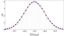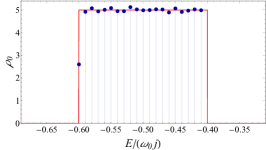
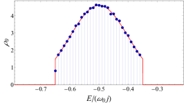
In Fig. 2, we show three cases of energy profiles of the initial state, one rectangular and two Gaussian profiles. The numerical results are obtained by averaging over ensembles of 500 initial states. The agreement with the analytical profiles from Eq. (8) and Eq. (11) confirms that 500 is a sufficiently large number to obtain stable results.

III.2 Survival Probability: Before the Correlation Hole

The energy distribution of $|\Psi(0)\rangle$ determines the initial decay of $S_{P}(t)$. This can be seen by expressing the survival probability in Eq. (4) as

$$S_{P}(t)=\left|\int\rho_{0}(E)e^{-iEt}dE\right|^{2},$$

where $\rho_{0}(E)=\sum_{k}|c_{k}|^{2}\delta(E-E_{k})$ is the local density of states (LDoS) or strength function, that is the energy distribution weighted by the components of the initial state. If we approximate the LDoS by its smoothed profile, $\rho_{0}(E)\approx\rho(E)$, we obtain for the rectangular profile,

$$S_{P}^{R}(t)=\frac{\sin^{2}(\sigma_{R}t)}{(\sigma_{R}t)^{2}},$$ (13)

and for the Gaussian profile,

$$S_{P}^{G}(t)=\dfrac{e^{-\sigma_{G}^{2}t^{2}}}{{4\cal C}^{2}}{\cal F}(t),\hskip 8.5359pt\text{with\ \ \ \ \ \ }$$ (14)

$${\cal F}(t)\!=\!\left|\textrm{erf}\left(\dfrac{E_{\textrm{c}}\!-\!E_{\textrm{min}}\!-\!i\sigma_{G}^{2}t}{\sqrt{2}\sigma_{G}}\right)\!-\!\textrm{erf}\left(\dfrac{E_{\textrm{c}}\!-\!E_{\textrm{max}}\!-\!i\sigma_{G}^{2}t}{\sqrt{2}\sigma_{G}}\right)\right|^{2}.$$

For very short times, $t\ll\sigma_{R,G}^{-1}$, both $S_{P}^{R}(t)$ and $S_{P}^{G}(t)$ show the universal quadratic decay of the survival probability $1-\sigma_{R,G}^{2}t^{2}$. For longer times, both profiles lead to a power-law decay $\propto t^{-2}$. This behavior is evident in Eq. (13) and it can be obtained from Eq. (14) by analyzing it at long times, in which case Távora et al. (2016, 2017),

$$S_{P}^{G}(t\gg\sigma_{G}^{-1})\approx\dfrac{1}{2\pi{\cal C}^{2}\sigma_{G}^{2}t^{2}}\times$$ (15)

$$\left\{{\cal E}-2e^{\!-\dfrac{\left[(E_{c}-E_{\textrm{min}})^{2}+(E_{\textrm{max}}-E_{c})^{2}\right]}{2\sigma_{G}^{2}}}\cos[(E_{\textrm{max}}-E_{\textrm{min}})t]\right\}\!\!,$$

where

$${\cal E}=\exp\left[{-\frac{(E_{\textrm{c}}-E_{\textrm{min}})^{2}}{\sigma_{G}^{2}}}\right]+\exp\left[{-\frac{(E_{\textrm{c}}-E_{\textrm{max}})^{2}}{\sigma_{G}^{2}}}\right].$$ (16)

Power-law decays of the survival probability are caused by the presence of energy bounds in the LDoS Khalfin (1958) and the power-law exponent depends on how the bounds are approached Urbanowski (2009).

III.3 Survival Probability: Analytical Expression

The expressions in Eqs. (13) and (14) describe accurately the initial decay of $S_{P}(t)$, for which just the shape and bounds of the envelope of $\rho_{0}(E)$ matters. However, the spectra of finite quantum systems are discrete and, in our case, the eigenvalues are correlated. This results in two additional features to the evolution of $S_{P}(t)$, beyond the power-law behavior, which are not captured by Eqs. (13) and (14). They are the manifestations of the spectrum correlations, which appear at long times, and the saturation of the dynamics to the asymptotic value

$$\bar{S}_{P}=\lim_{t\rightarrow\infty}\frac{1}{t}\int_{0}^{t}dt^{\prime}S_{P}(t^{\prime}),$$ (17)

around which the survival probability oscillates after relaxation.

To obtain an equation for the full dynamics, we write the survival probability as

$$S_{P}(t)=\sum_{k\neq l}|c_{l}|^{2}|c_{k}|^{2}e^{-i(E_{k}-E_{l})t}+I_{PR},$$ (18)

where

$$I_{PR}\equiv\sum_{k}|\langle\phi_{k}|\Psi(0)\rangle|^{4}=\bar{S}_{P}$$ (19)

is the so-called inverse participation ratio, which gives the asymptotic temporal value of $S_{P}(t)$. The $I_{PR}$ is a measure of the inverse of the number of elements of a given basis (the energy eigenbasis, in our case) participating in an arbitrary quantum state ($|\Psi(0)\rangle$, in our case).

For the considered ensembles of initial states, it is possible to derive accurate estimates for the ensemble averaged $\langle I_{PR}\rangle$ by using (see Appendix A)

$$\left\langle I_{PR}\right\rangle=\left\langle\frac{\sum_{k}r_{k}^{2}f^{2}(E_{k})}{\left(\sum_{q}r_{q}f(E_{q})\right)^{2}}\right\rangle\approx\frac{\langle{r_{k}^{2}\rangle}}{\langle r_{q}\rangle^{2}}\frac{1}{\nu_{c}}\int\rho^{2}(E)dE,$$ (20)

which, considering random variables $r_{k}$ uniformly distributed, gives for the rectangular profile,

$$\left\langle I_{PR}^{R}\right\rangle=\frac{2}{3\sigma_{R}\nu_{c}},$$ (21)

and for the Gaussian profile,

$$\left\langle I_{PR}^{G}\right\rangle=\frac{\textrm{erf}\left(\dfrac{E_{\textrm{c}}-E_{\textrm{min}}}{\sigma_{G}}\right)-\textrm{erf}\left(\dfrac{E_{\textrm{c}}-E_{\textrm{max}}}{\sigma_{G}}\right)}{3\sqrt{\pi}\sigma_{G}\nu_{c}{\cal C}^{2}}.$$ (22)

Above, $\nu_{c}=\nu(E_{c})$ is the DoS evaluated at the central energy $E_{c}$, which equals the inverse mean spacing of consecutive energy levels in the region probed by the initial state.

Since the components $c_{k}$ of the initial state are random numbers, to compute the ensemble average of $S_{P}(t)$, we can treat the statistical properties of the components and of the spectrum separately. Because the latter has level statistics comparable to that of random matrices from Gaussian orthogonal ensembles (GOE), as shown in Fig. 1 (a), we can follow steps similar to the ones described in Torres-Herrera et al. (2018); Schiulaz et al. to obtain (see Appendix A for details),

$$\left\langle S_{P}(t)\right\rangle=\frac{1-\left\langle I_{PR}\right\rangle}{\eta-1}\left[\eta S_{P}^{bc}(t)-b_{2}\left(\frac{t}{2\pi\nu_{c}}\right)\right]+\left\langle I_{PR}\right\rangle.$$ (23)

Above, $\eta$ is the effective dimension of the ensemble (see Appendix A) defined as,

$$\eta\equiv\frac{\nu_{c}}{\int\rho^{2}(E)dE}=\frac{\langle r_{k}^{2}\rangle}{\langle r_{k}\rangle^{2}}\frac{1}{\langle I_{PR}\rangle},$$ (24)

where the second equality is obtained using Eq. (20). In Eq. (23), $S_{P}^{bc}(t)$ describes the behavior of the survival probability before the manifestations of the correlations between the eigenvalues ($bc$ stands for “before correlations”), as given by Eqs. (13) and (14) for the rectangular and Gaussian profiles. This behavior holds until $\left\langle S_{P}(t)\right\rangle$ reaches its minimum value, which is actually below $\left\langle I_{PR}\right\rangle$. Beyond that, the dynamics becomes controlled by the two-level form factor,

$$b_{2}(\bar{t}) = [1-2\bar{t}+\bar{t}\ln(2\bar{t}+1)]\Theta(1-\bar{t})+$$ (25)

$$+ \left[\bar{t}\ln\left(\frac{2\bar{t}+1}{2\bar{t}-1}\right)-1\right]\Theta(\bar{t}-1),$$

where $\Theta$ is the Heaviside step function. The two-level form factor brings the survival probability from its minimum value up to the asymptotic value, creating the dip that is known as correlation hole Leviandier et al. (1986); Guhr and Weidenmüller (1990); Wilkie and Brumer (1991); Guhr et al. (1998); Alhassid and Levine (1992). The hole is a direct signature of the presence of correlated eigenvalues, and it does not develop in systems with uncorrelated eigenvalues. The equation used above for $b_{2}(\bar{t})$ is the same used for GOE full random matrices Mehta (1991). This implies that beyond the minimum of the correlation hole, the dynamics shows universal properties.

The analytical expression for the survival probability in Eq. (23) describes the complete evolution of $\left\langle S_{P}(t)\right\rangle$, from $t=0$ to saturation. The equation has no fitting parameters. All the parameters entering in Eq. (23) can be determined from the properties of the model and the energy profile of the initial state. As we show in the next section, this analytical expression shows remarkable agreement with our numerical results.

IV Comparing numerical and analytical results

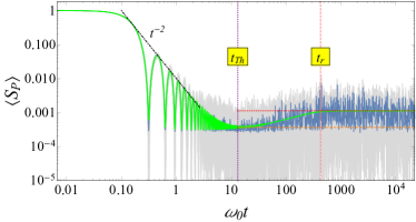
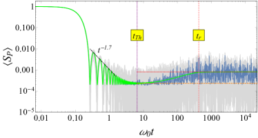
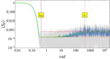
In Fig. 3, we compare numerical results for the survival probability with the analytical expression given by Eq. (23). The light (gray) lines represent the numerical results obtained with a single initial random state for the rectangular (a) and Gaussian [(b) and (c)] energy profiles. The darker (blue) line is obtained by performing ensemble averages over 500 random initial states. The bright (green) curve, following extremely well the ensemble average, is the analytical Eq. (23). As clear from all panels, the ensemble average is needed for the hole to be visible.

(a)	(b)
(c)	(d)

Figure 3: (Color online) Survival probability for the rectangular (a) [see Fig. 2 (a)], strongly bounded Gaussian (b) [see Fig. 2 (b)], and weakly bounded Gaussian (c) [see Fig. 2 (c)] energy profiles. In (a), (b), and (c): Light (gray) curves depict the survival probability for a single initial random state and the dark (blue) curve represents the ensemble average over 500 random initial states. The bright (green) line is the analytical expression in Eq. (23). The lowest horizontal dashed line is the analytical estimate for the minimum of the correlation hole (see text). The highest horizontal dotted line shows $\left\langle I_{PR}\right\rangle$, which is $1.106\times 10^{-3}$ for (a), $8.032\times 10^{-4}$ for (b), and $6.241\times 10^{-4}$ for (c). The leftmost vertical line indicates the analytical value for the time when the correlation hole attains its minimum value (Thouless time, $t_{Th}$). The rightmost vertical line marks the analytically evaluated relaxation time $t_{r}$. To determine $t_{r}$, we fixed $\delta=0.05$ in Eq. (37). In (a) and (b), the black dashed line indicates the power law decay $t^{-\lambda}$ for the initial oscillatory decay of $\left\langle S_{P}(t)\right\rangle$. Panel (d): The dark (blue) curves represent averages performed overt both initial states and temporal windows of constant size in logarithmic scale. From top to bottom, the curves are obtained with rectangular, strongly bounded Gaussian, and weakly bounded Gaussian energy profiles. The temporal averages are plotted against the mean value of the respective temporal windows. Bright (green) lines depict the same temporal averages of the analytical expression in Eq. (23).

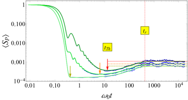The initial decay is determined entirely by the energy profile of the initial states, which is the same for every member of the ensemble. An oscillatory decay modulated by a power law $\propto t^{-\lambda}$ is seen in Figs. 3 (a) and (b). As mentioned before, this behavior is caused by the bounds in the energy profiles, which determine also the size of the oscillations. For the rectangular profile (a), the exponent is indeed $\lambda=2$, as obtained for $S_{P}^{bc}(t)$ in Eq. (13), whereas for the strongly bounded Gaussian profile (b), the power-law exponent obtained numerically is $\lambda=1.7$, instead of 2 as in Eq. (15). This is because the oscillations in Fig. 3 (b) start at a temporal scale where the two-level form factor $b_{2}$ is not negligible, so it affects the exponent. The power-law decay in Figs. 3 (a) and (b) is followed by the correlation hole. In the case of the weakly bounded Gaussian profile of panel (c), no trace of the modulated oscillations is left, because they occur at a temporal scale when $S_{P}^{bc}(t)$ is already extremely small with respect to the $b_{2}$ term. In all panels, once saturation is reached, the survival probability only fluctuates around its asymptotic value.

The minimum of the correlation hole is indicated in Figs. 3 (a), (b) and (c) with the lowest horizontal dashed line. The dynamics beyond this minimum point depends on level statistics, as confirmed by the fact that the behavior of the ensemble averages is very well described by the analytical expression (23), where the same two-level form factor $b_{2}$ used for full random matrices was employed. However, the size of the temporal fluctuations after the mimimum depends on the fine details of the particular spectrum and on the level of delocalization of the initial state written in the energy eigenbasis Reimann (2008); Short (2011); Short and Farrelly (2012); Zangara et al. (2013).

Contrary to ensembles of random matrices or disordered models, where one can further reduce the temporal fluctuations of $\left\langle S_{P}(t)\right\rangle$ with averages over many energy spectrum realizations, in the case of the Dicke model, the spectrum is exactly the same for every member of the ensemble. Thus, to further reduce the fluctuations in the ensemble averaged $\left\langle S_{P}(t)\right\rangle$, we perform an additional time average over temporal windows of constant size in logarithmic scale, i.e. temporal windows whose sizes increase exponentially in time. By plotting this temporal averages against the mean time of the respective windows, we obtain the results shown in Figs. 3 (d). This smoothing procedure results in numerical curves that are almost identical to the analytical curves, further validating Eq. (23) and the approach that led to it.

The fact that the dynamics beyond the minimum of the correlation hole is governed entirely by the two-level form factor implies that the time to reach saturation depends only on how the $b_{2}$ function approaches $\left\langle I_{PR}\right\rangle$ (indicated in Fig. 3 with the highest horizontal dashed line). Provided the initial state is fully extended in the energy eigenbasis, counting with the participation of all (most) energy levels in the energy interval characterizing $|\Psi(0)\rangle$, the relaxation time is independent of the initial state. Indeed, as seen in Fig. 3 (d), the time to reach $\left\langle I_{PR}\right\rangle$, which is shown with the rightmost vertical dashed line, is the same for the three different energy profiles.

V Timescales of the survival probability

In hands of the analytical expression for the survival probability, we can derive analytically the timescales involved in the relaxation process. We focus on the two longest timescales: the time to reach the minimum of the correlation hole, referred to as Thouless time $t_{Th}$, and the final relaxation time $t_{r}$.

V.1 Thouless Time

The Thouless time divides the dynamics of chaotic systems in two temporal regions, before $t_{Th}$ the dynamics is governed by the shape of the energy distribution of the initial state and the energy bounds, whereas after $t_{Th}$ the dynamics becomes comparable to that obtained with ensembles of full random matrices. The Thouless time marks the point where the term $\eta S_{P}^{bc}(t)$ in Eq. (23) meets the function $b_{2}(t/2\pi\nu_{c})$, being derived from

$$\left.\frac{d\left\langle S_{P}(t)\right\rangle}{dt}\right|_{t=t_{Th}}=0.$$ (26)

Therefore, we need to examine $S_{P}^{bc}(t)$ at long times and $b_{2}(t/2\pi\nu_{c})$ at short times, i.e. in the temporal range $\sigma^{-1}\ll t\ll\nu_{c}$ [recall that $\sigma$ is the width of the LDoS and $\nu_{c}$ is the inverse of the mean level spacing for the eigenvalues involved in the evolution of $|\Psi(0)\rangle$].

At long times, $\eta S_{P}^{bc}(t)$ shows a power-law decay $\propto t^{-2}$. More specifically, for the rectangular energy profile, the temporal average of the oscillatory decay in Eq. (13) leads to

$$\eta S_{P}^{bc,R}(t\gg\sigma_{R}^{-1})\rightarrow\frac{\eta}{2\sigma_{R}^{2}t^{2}}.$$ (27)

For the Gaussian profile, associated with Eq. (14), if the conditions

$$e^{-(E_{max}-E_{c})^{2}/\sigma^{2}}>\frac{1}{\eta}{\hbox{\ \ and\ \ }}e^{-(E_{min}-E_{c})^{2}/\sigma^{2}}>\frac{1}{\eta}$$ (28)

are fulfilled, the form of $S_{P}^{bc}(t)$ in the timescale where it meets $b_{2}$ is given by [see Eq. (15)]

$$\eta S_{P}^{bc,G}(t\gg\sigma_{G}^{-1})\rightarrow\frac{\eta{\cal E}}{2\pi{\cal C}^{2}\sigma_{G}^{2}t^{2}}.$$ (29)

This is what happens for the strongly bounded Gaussian energy profile of Fig. 2 (b). Otherwise, if the conditions in Eq. (28) are not fulfilled, the early Gaussian decay still persists at the meeting point with the $b_{2}$ function and

$$\eta S_{P}^{bc,G}(t\gg\sigma_{G}^{-1})\rightarrow\eta\exp[-\sigma_{G}^{2}t^{2}].$$ (30)

This is what happens for the weakly bounded Gaussian energy profile of Fig. 2 (c).

At short times, the two-level form factor is dominated by a linear term,

$$b_{2}\left(\frac{t}{2\pi\nu_{c}}\right)\rightarrow 1-\frac{t}{\pi\nu_{c}}\hskip 11.38092pt\text{for}\hskip 11.38092pt\frac{t}{\nu_{c}}\ll 1.$$ (31)

Combining Eqs. (27) and (31), we obtain the Thouless time for the rectangular ensemble

$$t_{Th}^{R}=\left(\frac{2\pi\nu_{c}^{2}}{\sigma_{R}}\right)^{1/3},$$ (32)

where we used that $\nu_{c}=\frac{\eta}{2\sigma_{R}}$ (see Eq. (24) and Appendix A). From Eq. (29) and Eq. (31), we arrive at the Thouless time for the strongly bounded Gaussian energy profile,

$$t_{Th}^{G}=\left(\frac{\eta\nu_{c}{\cal E}}{{\cal C}^{2}\sigma_{G}^{2}}\right)^{1/3}$$ (33)

and if the conditions (28) are not fulfilled, using Eq. (30), we have

$$t_{Th}^{G}\approx\frac{\sqrt{\log(2\pi\eta\sigma_{G}\nu_{c})}}{\sigma}.$$ (34)

The Thouless time obtained in the equations above are indicated in Fig. 3, showing excellent agreement with the numerics.

V.2 Relaxation Time

The relaxation time depends only on the $b_{2}$ function at long times, which grows toward saturation following a power-law behavior,

$$b_{2}\left(\frac{t}{2\pi\nu_{c}}\right)\rightarrow\frac{\pi^{2}\nu_{c}^{2}}{3t^{2}}\hskip 11.38092pt\text{for}\hskip 11.38092pt\frac{t}{\nu_{c}}\gg 1.$$ (35)

Even though Eq. (27) and Eq. (29) decay with the same power-law exponent 2, as in Eq. (35), the latter is proportional to $\eta^{2}$, since $\nu_{c}\propto\eta$, while the former equations are proportional to $\eta$, which justifies considering only Eq. (35). We define the relaxation time according to

$$\left\langle S_{P}(t_{r})\right\rangle=(1-\delta)\left\langle I_{PR}\right\rangle,$$ (36)

where $\delta$ is a small parameter determining the point where $\left\langle S_{P}(t)\right\rangle$ is already within the fluctuations around the asymptotic value. We arrive at

$$t_{r}=\frac{\pi\nu_{c}}{2\sqrt{\delta}},$$ (37)

which holds for the three energy profiles. This time is proportional to the inverse of the mean level spacing, $\nu_{c}$, which is the largest timescale of a quantum system and is known as the Heisenberg time. In Fig. 3, $t_{r}$ is indicated with the rightmost vertical lines, showing a excellent agreement with the numerical results.

V.3 Scaling with system size: Thouless and relaxation time

With Eqs. (32), (33), (34) and (37), we can determine the dependence of the Thouless and relaxation times on the size of the system, i.e on the number $\mathcal{N}=2j$ of two-level atoms. Both times depend on $\nu_{c}$, which scales linearly with $j$. We can write $\nu_{c}=\nu_{o}j/\omega$ and evaluate $\nu_{o}$ numerically, which for the chosen energy $E_{c}$ is $\nu_{o}=0.6027$.

The Thouless time depends additionally on the widths $\sigma_{R}$ and $\sigma_{G}$ of the energy distribution of the initial state and, for the Gaussian profile, on the energy bounds $E_{min}$ and $E_{max}$. The scaling $\sigma_{R,G}=\sigma_{R,G}^{o}j^{\beta}$ of these widths, as well as the scalings of $(E_{c}-E_{min})\propto j^{\alpha_{1}}$ and $(E_{max}-E_{c})\propto j^{\alpha_{2}}$, can in principle be selected at will in the range $-1\leq\beta\leq 1$ and $-1\leq\alpha_{i}\leq 1$. The lower values $\beta=\alpha_{i}=-1$ are imposed by the scaling of the mean-level spacing of consecutive energy levels and the upper bound is given by the scaling of the energy spectrum, which is proportional to $j$. A physical relevant choice for the previous scalings is $\beta=1/2$, which is the scaling of the energy widths of minimal uncertainty coherent states Schliemann (2015), and $\alpha_{i}=1$, which implies that the bounding energy interval of the Gaussian profile scales as the energy spectrum. Therefore for the rectangular profile and strongly bounded Gaussian profile satisfying conditions (28), the Thouless time scales as

$$t_{Th}^{R,G}=t_{o}^{R,G}j^{1/2},$$ (38)

where $t_{o}^{R,G}$ is a constant determined by $\nu_{o}$, and $\sigma_{R,G}^{o}$. For the rectangular profile, this scaling is valid for any $j$, but for the Gaussian profile, it is valid up to a finite value of $j$. This is because we assume that $(E_{c}-E_{min})$ and $(E_{max}-E_{c})$ grow with $j$ faster than $\sigma_{G}$, which implies that for large enough $j$ the conditions (28) will not be satisfied anymore, switching to the scenario of Eq. (34). For the weakly bounded Gaussian profile, described by Eq. (34), the Thouless time for large $j$ is given by,

$$t_{Th}^{G}=\frac{\sqrt{\log c_{o}+3\log j}}{\sigma_{G}^{o}j^{1/2}},$$ (39)

where $c_{o}=4\pi^{(3/2)}(\sigma_{G}^{o})^{2}\nu_{o}^{2}/\omega^{2}$, and we have approximated the error functions by their asymptotic values, $\lim_{z\rightarrow\infty}\textrm{erf}(z)\rightarrow 1$.

The relaxation time is independent of the details of the initial state and scales linearly with $\nu_{c}$, so it is given simply by

$$t_{r}=\frac{\pi\nu_{o}}{2\omega\sqrt{\delta}}j.$$ (40)

The distance between the Thouless and the relaxation time diverge with $j$, which means that the correlation hole gets elongated as the number of atoms increases.

V.4 Depth of the correlation hole

With the Thouless time, we can quantify the relative depth of the correlation hole through the expression

$$\kappa=\frac{\left\langle I_{PR}\right\rangle-\left\langle S_{P}(t_{Th})\right\rangle}{\left\langle I_{PR}\right\rangle}.$$ (41)

For the ensembles considered in this paper, we can calculate the depth of the correlation hole for $j\gg 1$. A direct substitution of the Thouless time in the analytical expression for the survival probability in Eq. (23) allows to demonstrate that

$$\lim_{j\gg 1}\left\langle S_{P}(t_{Th})\right\rangle=-\frac{1}{\eta}+\left\langle I_{PR}\right\rangle=\frac{\langle r_{k}^{2}\rangle-\langle r_{k}\rangle^{2}}{\langle r_{k}^{2}\rangle}\left\langle I_{PR}\right\rangle,$$

where in the last step we have used Eq. (24). From this result, we obtain

$$\kappa_{\infty}=\frac{\langle r_{k}\rangle^{2}}{\langle r_{k}^{2}\rangle}.$$ (42)

The value $\kappa_{\infty}$ gives an upper bound for the depth of the correlation hole for finite $j$. In the case of random variables $r_{k}$ uniformly distributed in the interval $[0,1]$, as considered here noteGOE , this bound is $\kappa_{\infty}=3/4$.

The actual values of $\kappa$ for the finite systems studied, where $j=100$, are obtained by substituting Eqs. (32), (33) and (34) in Eq. (23), which gives $\left\langle S_{P}(t_{Th})\right\rangle$, and by getting $\left\langle I_{PR}\right\rangle$ from Eqs. (21) and (22). We get $\kappa=0.672$ for the rectangular ensemble, $\kappa=0.711$ for the ensemble from the strongly bounded Gaussian profile, and $\kappa=0.748$ for the ensemble from the weakly bounded Gaussian profile. The analytical estimates for $\left\langle S_{P}(t_{Th})\right\rangle$ and $\left\langle I_{PR}\right\rangle$ are depicted in Fig. 3 (a), (b), and (c) with horizontal lines, showing excellent agreement with the numerical results. This confirms that the analytical expression in Eq. (23) describes the survival probability at any timescale.

VI CONCLUSIONS

We obtained an analytical expression that describes remarkably well the entire evolution of the averaged survival probability, $\langle S_{P}(t)\rangle$, for the Dicke model in the chaotic regime and allowed us to derive analytical expressions for the different timescales involved in the relaxation to equilibrium. Due to spectral correlations, the survival probability exhibits a correlation hole. We find that the initial decay of $\langle S_{P}(t)\rangle$ and the time $t_{Th}$ for it to reach the minimum of the correlation hole (Thouless time) depend on the energy profile of the initial states. Beyond the Thouless time, the dynamics is universal, being governed by the two-level form factor of the GOE. This implies that the time, $t_{r}$, for the survival probability to reach equilibrium (relaxation time) depends only on the energies, being proportional to the inverse of the mean level spacing. An interesting future direction would be to investigate the timescales involved in the relaxation process of other physical observables that are relevant for the Dicke model.

Appendix A Ensemble averages of the survival probability

In this appendix we present the steps involved in the derivation of the analytical expression given by Eq. (23) for the ensemble average of the survival probability. We begin with Eq. (18) and perform ensemble averages, taking into account that the eigenvalues and the components $|c_{k}|^{2}$ of the initial state are statistically independent,

$$\langle S_{P}(t)\rangle = \left\langle\sum_{k\neq l}|c_{l}|^{2}|c_{k}|^{2}e^{-i(E_{k}-E_{l})t}\right\rangle+\left\langle I_{PR}\right\rangle$$ (43)

$$= \sum_{k\neq l}\left\langle|c_{l}|^{2}|c_{k}|^{2}\right\rangle e^{-i(E_{k}-E_{l})t}+\left\langle I_{PR}\right\rangle.$$

Let us consider first the ensemble average of $I_{PR}$. Using Eq. (5), we have

$$\left\langle I_{PR}\right\rangle = \left\langle\sum_{k}|c_{k}|^{4}\right\rangle=\left\langle\frac{\sum_{k}r_{k}^{2}f^{2}(E_{k})}{\left(\sum_{q}r_{q}f(E_{q})\right)^{2}}\right\rangle$$ (44)

$$= \sum_{k}\left\langle\frac{r_{k}^{2}}{\left(\sum_{q}r_{q}f(E_{q})\right)^{2}}\right\rangle f^{2}(E_{k}).$$

For a large number of components, the average of the second line above can be approximated as

$$\left\langle\frac{r_{k}^{2}}{\left(\sum_{q}r_{q}f(E_{q})\right)^{2}}\right\rangle \approx \frac{\langle r_{k}^{2}\rangle}{\left(\sum_{q}\langle r_{q}\rangle f(E_{q})\right)^{2}}$$ (45)

$$= \frac{\langle r_{k}^{2}\rangle}{\langle r_{q}\rangle^{2}}\frac{1}{\left(\sum_{q}f(E_{q})\right)^{2}},$$

where in the last equality we have used the fact that $\langle r_{q}^{n}\rangle$ is actually independent of index $q$. By inserting this result in Eq. (44), we obtain

$$\left\langle I_{PR}\right\rangle=\frac{\langle r_{k}^{2}\rangle}{\langle r_{q}\rangle^{2}}\frac{\sum_{k}f^{2}(E_{k})}{\left(\sum_{q}f(E_{q})\right)^{2}}\equiv\frac{\langle r_{k}^{2}\rangle}{\langle r_{q}\rangle^{2}}\frac{1}{\eta}.$$ (46)

Here, we have introduced the effective dimension of the ensemble

$$\eta=\frac{\left(\sum_{q}f(E_{q})\right)^{2}}{\sum_{k}f^{2}(E_{k})},$$ (47)

whose name comes from the fact that it reduces to the number of states participating in the rectangular ensemble, as it is shown below. We now approximate the sums in Eq. (46) by integrals,

$$\sum_{k}\bullet\rightarrow\int dE\,\nu(E)\bullet,$$ (48)

to obtain

$$\left\langle I_{PR}\right\rangle\approx\frac{\langle r_{k}^{2}\rangle}{\langle r_{q}\rangle^{2}}\frac{\int dE\,\rho^{2}(E)/\nu(E)}{\left(\int dE\,\rho(E)\right)^{2}}=\frac{\langle r_{k}^{2}\rangle}{\langle r_{q}\rangle^{2}}\int dE\,\frac{\rho^{2}(E)}{\nu(E)},$$

where we have used $f(E)=\rho(E)/\nu(E)$, and, in the last equality, the normalization of $\rho(E)$. Finally, since $\nu(E)$ varies linearly in the energy interval where $\rho(E)$ is significant, we substitute the function $\nu(E)$ by its value in the center of the profile distribution $\nu_{c}\equiv\nu(E_{c})$ and obtain

$$\left\langle I_{PR}\right\rangle\approx\frac{\langle r_{k}^{2}\rangle}{\langle r_{q}\rangle^{2}}\frac{1}{\nu_{c}}\int dE\,\rho^{2}(E),$$

and

$$\eta=\frac{\nu_{c}}{\int dE\,\rho^{2}(E)}.$$

From the expression for $\eta$, it is clear that, in the case of the rectangular profile $\eta=2\nu_{c}\sigma_{R}$, which gives the number of states participating in the ensemble.

For the first term in Eq (43), we have to evaluate the ensemble average

$$\left\langle|c_{l}|^{2}|c_{k}|^{2}\right\rangle=f_{l}f_{k}\left\langle\frac{r_{l}r_{k}}{\left(\sum_{q}r_{q}f_{q}\right)^{2}}\right\rangle$$

where $(l\not=k)$ and, for simplicity, we introduced the shorthand notation $f_{k}\equiv f(E_{k})$. To obtain an approximation to the average, we consider the identity,

$$1=\frac{\sum_{k}f_{k}r_{k}\sum_{l}f_{l}r_{l}}{\left(\sum_{q}r_{q}f_{q}\right)^{2}}=\frac{\sum_{k}f_{k}^{2}r_{k}^{2}}{\left(\sum_{q}r_{q}f_{q}\right)^{2}}+\frac{\sum_{l\not=k}r_{l}r_{k}f_{l}f_{k}}{\left(\sum_{q}r_{q}f_{q}\right)^{2}}.$$

From this, we obtain

$$\frac{\sum_{l\not=k}r_{l}r_{k}f_{l}f_{k}}{\left(\sum_{q}r_{q}f_{q}\right)^{2}}=1-I_{PR}.$$

By taking the ensemble average of this expression and assuming that

$$\left\langle\frac{r_{l}r_{k}}{\left(\sum_{q}r_{q}f_{q}\right)^{2}}\right\rangle\approx A,$$

where $A$ is a constant independent of indexes $l$ and $k$, we get

$$A\sum_{l\not=k}f_{l}f_{k}=1-\langle{I}_{PR}\rangle,$$

which implies that

$$A=\frac{1-\langle{I}_{PR}\rangle}{\sum_{l\not=k}f_{l}f_{k}}.$$

The sum in the denominator of the equation above can be expressed in terms of the effective dimension $\eta$ [see Eq. (47)], as follows

$$\sum_{l\not=k}f_{l}f_{k}=\frac{\eta-1}{\eta}\left(\sum_{q}f_{q}\right)^{2}=\frac{\eta-1}{\eta},$$

where in the last step, the normalization $\sum_{q}f_{q}\rightarrow\int dE\rho(E)=1$ was used. With the the above result, the average can be written as

$$\left\langle|c_{l}|^{2}|c_{k}|^{2}\right\rangle\approx\frac{1-\langle I_{PR}\rangle}{\eta-1}\eta f_{l}f_{k},$$

which, when substituted in Eq. (43), leads to

$$\langle S_{P}(t)\rangle=\langle I_{PR}\rangle+\frac{1-\langle I_{PR}\rangle}{\eta-1}\eta\sum_{k\neq l}f_{k}f_{l}e^{-i(E_{k}-E_{l})t}.$$ (49)

We now turn our attention to the double sum $\sum_{k\neq l}$ in Eq. (49). To solve it, we use

$$\sum_{k\not=l}\bullet\rightarrow\int dEdE^{\prime}R(E,E^{\prime})\bullet,$$

where the Dyson two-point correlation function, $R(E,E^{\prime})=\nu(E)\nu(E^{\prime})-T(E-E^{\prime})$, includes the DoS, $\nu(E)$, and the two-level cluster function, $T(E-E^{\prime})$, which has information about the correlations between the eigenvalues Mehta (1991). We then obtain

$$\sum_{k\neq l}f_{k}f_{l}e^{-i(E_{k}-E_{l})t}\rightarrow\left|\int\rho(E)e^{-iEt}dE\right|^{2}$$

$$-\int dEdE^{\prime}\rho(E)\rho(E^{\prime})\frac{T(E-E^{\prime})}{\nu(E)\nu(E^{\prime})}e^{-i(E-E^{\prime})t}.$$ (50)

Using unfolded energy variables, which leads to universal functions in the limit of an infinite number of levels, we have Mehta (1991)

$$Y\left([E-E^{\prime}]\nu_{c}\right)=T(E-E^{\prime})/\nu_{c}^{2}.$$

With this function, the second integral in Eq. (50) is

$$\int dEdE^{\prime}\rho(E)\rho(E^{\prime})\frac{T(E-E^{\prime})}{\nu(E)\nu(E^{\prime})}e^{-i(E-E^{\prime})t}\approx$$

$$\int dEdE^{\prime}\rho(E)\rho(E^{\prime})Y\left([E-E^{\prime}]\nu_{c}\right)e^{-i(E-E^{\prime})t},$$ (51)

which, in terms of variables $z=E^{\prime}$ and $x=(E-E^{\prime})\nu_{c}$ becomes

$$\frac{1}{\nu_{c}}\int dxdz\rho(z)\rho(z+x/\nu_{c})Y(x)e^{-i2\pi x\tilde{t}}$$ (52)

with $\tilde{t}=t/(2\pi\nu_{c})$. By expanding $\rho(z+x/\nu_{c})$ in powers of $x$ and considering only the lowest order, the double integral can be approximated by a product of two independent integrals

$$\frac{1}{\nu_{c}}\int dz\rho(z)^{2}\int dxY(x)e^{-i2\pi x\tilde{t}}=\frac{1}{\eta}b_{2}\left(\frac{t}{2\pi\nu_{c}}\right),$$

where we have used the effective dimension introduced before, and $b_{2}(\tilde{t})$ is the known Fourier transform of the GOE-two level cluster function Mehta (1991), the so called two-level form factor shown in Eq. (25). We use the same $b_{2}(\tilde{t})$ as in GOE matrices, because the unfolded spectrum of the Dicke model has correlations comparable to those of the GOE levels.

Gathering the previous results together, we obtain for the ensemble average of the survival probability

$$\langle S_{P}(t)\rangle = \langle I_{PR}\rangle+$$ (53)

$$\frac{1-\langle I_{PR}\rangle}{\eta-1} \left[\eta\left|\int\rho(E)e^{-iEt}dE\right|^{2}-b_{2}\left(\frac{t}{2\pi\nu_{c}}\right)\right].$$

Since the squared absolute value inside the parenthesis is the short time decay $S_{p}^{bc}$ given by Eqs. (13) and (14), we finally arrive at our analytical expression in Eq. (23).

References

- Reimann (2008) Peter Reimann, “Foundation of statistical mechanics under experimentally realistic conditions,” Phys. Rev. Lett. 101, 190403 (2008).
- Short (2011) A. J. Short, “Equilibration of quantum systems and subsystems,” New J. Phys. 13, 053009 (2011).
- Short and Farrelly (2012) A. J. Short and T. C. Farrelly, “Quantum equilibration in finite time,” New J. Phys. 14, 013063 (2012).
- Zangara et al. (2013) Pablo R. Zangara, Axel D. Dente, E. J. Torres-Herrera, Horacio M. Pastawski, A. Iucci, and Lea F. Santos, “Time fluctuations in isolated quantum systems of interacting particles,” Phys. Rev. E 88, 032913 (2013).
- He et al. (2013) K. He, L. F. Santos, T. M. Wright, and M. Rigol, “Single-particle and many-body analyses of a quasiperiodic integrable system after a quench,” Phys. Rev. A 87, 063637 (2013).
- Gogolin and Eisert (2016) C. Gogolin and J. Eisert, “Equilibration, thermalisation, and the emergence of statistical mechanics in closed quantum systems,” Rep. Prog. Phys. 79, 056001 (2016).
- Borgonovi et al. (2016) F. Borgonovi, F. M. Izrailev, L. F. Santos, and V. G. Zelevinsky, “Quantum chaos and thermalization in isolated systems of interacting particles,” Phys. Rep. 626, 1 (2016).
- Alessio et al. (2016) L. D’ Alessio, Y. Kafri, A. Polkovnikov, and M. Rigol, “From quantum chaos and eigenstate thermalization to statistical mechanics and thermodynamics,” Adv. Phys. 65, 239–362 (2016).
- Dymarsky (a) A. Dymarsky, “Bound on eigenstate thermalization from transport,” arXiv:1804.08626.
- Reimann (2018a) P. Reimann, “Dynamical typicality approach to eigenstate thermalization,” Phys. Rev. Lett. 120, 230601 (2018a).
- Reimann (2018b) P. Reimann, “Dynamical typicality of isolated many-body quantum systems,” Phys. Rev. E 97, 062129 (2018b).
- Monnai (2013) Takaaki Monnai, “Generic evaluation of relaxation time for quantum many-body systems: Analysis of the system size dependence,” J. Phys. Soc. Jpn. 82, 044006 (2013).
- Goldstein et al. (2013) Sheldon Goldstein, Takashi Hara, and Hal Tasaki, “Time scales in the approach to equilibrium of macroscopic quantum systems,” Phys. Rev. Lett. 111, 140401 (2013).
- Malabarba et al. (2014) Artur S. L. Malabarba, Luis Pedro García-Pintos, Noah Linden, Terence C. Farrelly, and Anthony J. Short, “Quantum systems equilibrate rapidly for most observables,” Phys. Rev. E 90, 012121 (2014).
- Goldstein et al. (2015) Sheldon Goldstein, Takashi Hara, and Hal Tasaki, “Extremely quick thermalization in a macroscopic quantum system for a typical nonequilibrium subspace,” New J. Phys. 17, 045002 (2015).
- Reimann (2016) Peter Reimann, “Typical fast thermalization processes in closed many-body systems,” Nat. Comm. 7, 10821 (2016).
- García-Pintos et al. (2017) Luis Pedro García-Pintos, Noah Linden, Artur S. L. Malabarba, Anthony J. Short, and Andreas Winter, “Equilibration time scales of physically relevant observables,” Phys. Rev. X 7, 031027 (2017).
- de Oliveira et al. (2018) Thiago R de Oliveira, Christos Charalambous, Daniel Jonathan, Maciej Lewenstein, and Arnau Riera, “Equilibration time scales in closed many-body quantum systems,” New J. Phys. 20, 033032 (2018).
- Dymarsky (b) A. Dymarsky, “Mechanism of slow equilibration of isolated quantum systems,” arXiv:1806.04187.
- Chan et al. (2018) A. Chan, A. De Luca, and J. T. Chalker, “Spectral statistics in spatially extended chaotic quantum many-body systems,” Phys. Rev. Lett. 121, 060601 (2018).
- Bertini et al. (2018) Bruno Bertini, Pavel Kos, and Tomaž Prosen, “Exact spectral form factor in a minimal model of many-body quantum chaos,” Phys. Rev. Lett. 121, 264101 (2018).
- (22) Mauro Schiulaz, E. J. Torres-Herrera, and Lea F. Santos, “Thouless and relaxation timescales in many-body quantum systems,” arXiv:1807.07577.
- Borgonovi et al. (2019) Fausto Borgonovi, Felix M. Izrailev, and Lea F. Santos, “Exponentially fast dynamics of chaotic many-body systems,” Phys. Rev. E 99, 010101 (2019).
- Berry (1983) M. V. Berry, “Semi-classical mechanics of regular and irregular motion,” in Les Houches Summer School 1981 on Chaotic Behaviour of Deterministic Systems, edited by G. Iooss, H.G. Helleman, and R. Stora (North-Holland, Amsterdam, 1983) p. 171.
- (25) The survival probability is also called return probability, autocorrelation function, or fidelity. It has also been called “Loschmidt echo”, but this term is not appropriate since the survival probability does not involve any time reversal Goussev et al. (2012).
- (26) A hole appears for observables that decrease in time and a bulge in the case of quantities, such as entropies, that increase in time Torres-Herrera and Santos (2017a).
- Leviandier et al. (1986) Luc Leviandier, Maurice Lombardi, Rémi Jost, and Jean Paul Pique, “Fourier transform: A tool to measure statistical level properties in very complex spectra,” Phys. Rev. Lett. 56, 2449–2452 (1986).
- Guhr and Weidenmüller (1990) T. Guhr and H.A. Weidenmüller, “Correlations in anticrossing spectra and scattering theory. analytical aspects,” Chem. Phys. 146, 21 – 38 (1990).
- Wilkie and Brumer (1991) Joshua Wilkie and Paul Brumer, “Time-dependent manifestations of quantum chaos,” Phys. Rev. Lett. 67, 1185–1188 (1991).
- Alhassid and Levine (1992) Y. Alhassid and R. D. Levine, “Spectral autocorrelation function in the statistical theory of energy levels,” Phys. Rev. A 46, 4650–4653 (1992).
- Torres-Herrera and Santos (2017a) E. J. Torres-Herrera and Lea F. Santos, “Extended nonergodic states in disordered many-body quantum systems,” Ann. Phys. (Berlin) 529, 1600284 (2017a).
- Torres-Herrera and Santos (2017b) E. J. Torres-Herrera and Lea F. Santos, “Dynamical manifestations of quantum chaos: correlation hole and bulge,” Philos. Trans. Royal Soc. A 375, 20160434 (2017b).
- Torres-Herrera et al. (2018) E. J. Torres-Herrera, Antonio M. García-García, and Lea F. Santos, “Generic dynamical features of quenched interacting quantum systems: Survival probability, density imbalance, and out-of-time-ordered correlator,” Phys. Rev. B 97, 060303 (2018).
- Torres-Herrera and Santos (2019) E. J. Torres-Herrera and Lea F. Santos, “Signatures of chaos and thermalization in the dynamics of many-body quantum systems,” Eur. Phys. J. Spec. Top. 227, 1897 (2019).
- Cotler et al. (2017) J. Cotler, N. Hunter-Jones, J. Liu, and B. Yoshida, “Chaos, complexity, and random matrices,” J. High Energy Phys. 2017, 48 (2017).
- Gharibyan et al. (2018) Hrant Gharibyan, Masanori Hanada, Stephen H. Shenker, and Masaki Tezuka, “Onset of random matrix behavior in scrambling systems,” Journal of High Energy Physics 2018, 124 (2018).
- Nosaka et al. (2018) Tomoki Nosaka, Dario Rosa, and Junggi Yoon, “The Thouless time for mass-deformed SYK,” Journal of High Energy Physics 2018, 41 (2018).
- Brody et al. (1981) T. A. Brody, J. Flores, J. B. French, P. A. Mello, A. Pandey, and S. S. M. Wong, “Random-matrix physics: spectrum and strength fluctuations,” Rev. Mod. Phys. 53, 385 (1981).
- (39) E. J. Torres-Herrera, J. A. Méndez-Bermúdez, and Lea F. Santos, “Level Repulsion and Dynamics in the Finite One-Dimensional Anderson Model”, arXiv: 1904.11989.
- Dicke (1954) R. H. Dicke, “Coherence in spontaneous radiation processes,” Phys. Rev. 93, 99–110 (1954).
- Garraway (2011) Barry M. Garraway, “The dicke model in quantum optics: Dicke model revisited,” Philos. Trans. Royal Soc. A 369, 1137 (2011).
- Baumann et al. (2010) Kristian Baumann, Christine Guerlin, Ferdinand Brennecke, and Tilman Esslinger, “Dicke quantum phase transition with a superfluid gas in an optical cavity,” Nature (London) 464, 1301 (2010).
- Baumann et al. (2011) K. Baumann, R. Mottl, F. Brennecke, and T. Esslinger, “Exploring symmetry breaking at the Dicke quantum phase transition,” Phys. Rev. Lett. 107, 140402 (2011).
- Lewenkopf et al. (1991) C.H Lewenkopf, M.C Nemes, V Marvulle, M.P Pato, and W.F Wreszinski, “Level statistics transitions in the spin-boson model,” Phys. Lett. A 155, 113 – 116 (1991).
- Emary and Brandes (2003a) Clive Emary and Tobias Brandes, “Quantum chaos triggered by precursors of a quantum phase transition: The Dicke model,” Phys. Rev. Lett. 90, 044101 (2003a).
- Emary and Brandes (2003b) Clive Emary and Tobias Brandes, “Chaos and the quantum phase transition in the Dicke model,” Phys. Rev. E 67, 066203 (2003b).
- Bastarrachea-Magnani et al. (2014a) M. A. Bastarrachea-Magnani, S. Lerma-Hernández, and J. G. Hirsch, “Comparative quantum and semiclassical analysis of atom-field systems. ii. Chaos and regularity,” Phys. Rev. A 89, 032102 (2014a).
- Bastarrachea-Magnani et al. (2015) Miguel Angel Bastarrachea-Magnani, Baldemar López del Carpio, Sergio Lerma-Hernández, and Jorge G Hirsch, “Chaos in the Dicke model: quantum and semiclassical analysis,” Phys. Scripta 90, 068015 (2015).
- Bastarrachea-Magnani et al. (2016) M. A. Bastarrachea-Magnani, B. López-del-Carpio, J. Chávez-Carlos, S. Lerma-Hernández, and J. G. Hirsch, “Delocalization and quantum chaos in atom-field systems,” Phys. Rev. E 93, 022215 (2016).
- Chávez-Carlos et al. (2016) J. Chávez-Carlos, M. A. Bastarrachea-Magnani, S. Lerma-Hernández, and J. G. Hirsch, “Classical chaos in atom-field systems,” Phys. Rev. E 94, 022209 (2016).
- (51) Gian Marcello Andolina, Maximilian Keck, Andrea Mari, Vittorio Giovannetti, and Marco Polini, “Quantum versus classical many-body batteries,” arXiv:1812.04669.
- Pérez-Fernández et al. (2011a) P. Pérez-Fernández, A. Relaño, J. M. Arias, P. Cejnar, J. Dukelsky, and J. E. García-Ramos, “Excited-state phase transition and onset of chaos in quantum optical models,” Phys. Rev. E 83, 046208 (2011a).
- Brandes (2013) Tobias Brandes, “Excited-state quantum phase transitions in Dicke superradiance models,” Phys. Rev. E 88, 032133 (2013).
- Bastarrachea-Magnani et al. (2014b) M. A. Bastarrachea-Magnani, S. Lerma-Hernández, and J. G. Hirsch, “Comparative quantum and semiclassical analysis of atom-field systems. I. Density of states and excited-state quantum phase transitions,” Phys. Rev. A 89, 032101 (2014b).
- Larson and Irish (2017) Jonas Larson and Elinor K Irish, “Some remarks on superradiant phase transitions in light-matter systems,” J. Phys. A 50, 174002 (2017).
- Pérez-Fernández et al. (2011b) P. Pérez-Fernández, P. Cejnar, J. M. Arias, J. Dukelsky, J. E. García-Ramos, and A. Relaño, “Quantum quench influenced by an excited-state phase transition,” Phys. Rev. A 83, 033802 (2011b).
- Altland and Haake (2012) Alexander Altland and Fritz Haake, “Quantum chaos and effective thermalization,” Phys. Rev. Lett. 108, 073601 (2012).
- Lerma-Hernández et al. (2018) Sergio Lerma-Hernández, Jorge Chávez-Carlos, Miguel A. Bastarrachea-Magnani, Lea F. Santos, and Jorge G. Hirsch, “Analytical description of the survival probability of coherent states in regular regimes,” J. Phys. A 51, 475302 (2018).
- Kloc et al. (2018) Michal Kloc, Pavel Stránský, and Pavel Cejnar, “Quantum quench dynamics in Dicke superradiance models,” Phys. Rev. A 98, 013836 (2018).
- Chávez-Carlos et al. (2019) Jorge Chávez-Carlos, B. López-del Carpio, Miguel A. Bastarrachea-Magnani, Pavel Stránský, Sergio Lerma-Hernández, Lea F. Santos, and Jorge G. Hirsch, “Quantum and classical lyapunov exponents in atom-field interaction systems,” Phys. Rev. Lett. 122, 024101 (2019).
- Baden et al. (2014) Markus P. Baden, Kyle J. Arnold, Arne L. Grimsmo, Scott Parkins, and Murray D. Barrett, “Realization of the Dicke model using cavity-assisted raman transitions,” Phys. Rev. Lett. 113, 020408 (2014).
- Klinder et al. (2015) J. Klinder, H. Keßler, M. Reza Bakhtiari, M. Thorwart, and A. Hemmerich, “Observation of a superradiant mott insulator in the Dicke-hubbard model,” Phys. Rev. Lett. 115, 230403 (2015).
- Cohn et al. (2018) J Cohn, A Safavi-Naini, R J Lewis-Swan, J G Bohnet, M Gärttner, K A Gilmore, J E Jordan, A M Rey, J J Bollinger, and J K Freericks, “Bang-bang shortcut to adiabaticity in the dicke model as realized in a penning trap experiment,” New J. Phys. 20, 055013 (2018).
- Blatt and Roos (2012) R. Blatt and C. F. Roos, “Quantum simulations with trapped ions,” Nat. Phys. 8, 277–284 (2012).
- Hepp and Lieb (1973a) Klaus Hepp and Elliott H Lieb, “On the superradiant phase transition for molecules in a quantized radiation field: the Dicke maser model,” Ann. Phys. (N.Y.) 76, 360 – 404 (1973a).
- Hepp and Lieb (1973b) Klaus Hepp and Elliott H. Lieb, “Equilibrium statistical mechanics of matter interacting with the quantized radiation field,” Phys. Rev. A 8, 2517–2525 (1973b).
- (67) G. Casati, F. Valz-Gris, and I. Guarnieri, “On the connection between quantization of nonintegrable systems and statistical theory of spectra”, Lett. Nuovo Cimento 28, 279 (1980).
- (68) O. Bohigas, M. J. Giannoni, and C. Schmit, “Characterization of Chaotic Quantum Spectra and Universality of Level Fluctuation Laws”, Phys. Rev. Lett. 52, 1 (1984).
- Guhr et al. (1998) T. Guhr, A. Mueller-Gröeling, and H. A. Weidenmüller, “Random matrix theories in quantum physics: Common concepts,” Phys. Rep. 299, 189 (1998).
- Bastarrachea-Magnani and Hirsch (2014) Miguel A Bastarrachea-Magnani and Jorge G Hirsch, “Efficient basis for the Dicke model: I. Theory and convergence in energy,” Phys. Scripta 2014, 014005 (2014).
- Hirsch and Bastarrachea-Magnani (2014) Jorge G Hirsch and Miguel A Bastarrachea-Magnani, “Efficient basis for the Dicke model: II. Wave function convergence and excited states,” Phys. Scripta 2014, 014018 (2014).
- Torres-Herrera and Santos (2014) E. J. Torres-Herrera and Lea F. Santos, “Quench dynamics of isolated many-body quantum systems,” Phys. Rev. A 89, 043620 (2014).
- Khalfin (1958) L. A. Khalfin, “Contribution to the decay theory of a quasi-stationary state,” Sov. Phys. JETP 6, 1053 (1958).
- Fonda et al. (1978) L. Fonda, G. C. Ghirardi, and A. Rimini, “Decay theory of unstable quantum systems,” Rep. Prog. Phys. 41, 587 (1978).
- Bhattacharyya (1983) K. Bhattacharyya, “Quantum decay and the mandelstam-tamm-energy inequality,” J. Phys. A 16, 2993 (1983).
- Muga et al. (2009) J. G. Muga, A. Ruschhaupt, and A. del Campo, Time in Quantum Mechanics, vol. 2 (Springer, London, 2009).
- Távora et al. (2016) Marco Távora, E. J. Torres-Herrera, and Lea F. Santos, “Inevitable power-law behavior of isolated many-body quantum systems and how it anticipates thermalization,” Phys. Rev. A 94, 041603 (2016).
- Távora et al. (2017) Marco Távora, E. J. Torres-Herrera, and Lea F. Santos, “Power-law decay exponents: A dynamical criterion for predicting thermalization,” Phys. Rev. A 95, 013604 (2017).
- Urbanowski (2009) K. Urbanowski, “General properties of the evolution of unstable states at long times,” Eur. Phys. J. D 54, 25–29 (2009).
- Mehta (1991) M. L. Mehta, Random Matrices (Academic Press, Boston, USA, 1991).
- Schliemann (2015) John Schliemann, “Coherent quantum dynamics: What fluctuations can tell,” Phys. Rev. A 92, 022108 (2015).
- (82) We note that for random variables , where come from a Gaussian probability distribution, Eq. (42) gives , which is the depth obtained for full random matrices from GOE Torres-Herrera and Santos (2017b).
- Goussev et al. (2012) A. Goussev, R. A. Jalabert, H. M. Pastawski, and D. A. Wisniacki, “Loschmidt echo,” Scholarpedia 7, 11687 (2012).