Spurious pressure in Scott-Vogelius elements

Abstract

We will analyze the characteristics of Scott-Vogelius finite elements on singular vertices, which cause spurious pressures on solving Stokes equations. A simple postprocessing will be suggested to remove those spurious pressures.

1 Introduction

The Scott-Vogelius element is the typical high order finite element space which can be applied to solve Stokes problems. Its inf-sup condition was proved in several ways, only when the triangulation has no singular vertex [5, 6, 9]. While it struggles with singular vertices, the inf-sup constant $\beta$ is not proper even in case of nearly singular vertices.

In practice, when the mesh has a nearly singular vertex, the discrete solution in pressure shows an error which is improper at a glance as in Figure 15 in the numerical test section. In this paper, we will call it spurious and analyze its causes.

The punchline of the paper is splitting of the error in stable and unstable parts on nearly singular vertices. We will suggest a simple postprocessing to remove the unstable parts from the discrete pressure obtained by the standard finite element methods. The suggested postprocessing could improve the error even in case of regular vertices.

In our analysis, a cubic polynomial depicted in Figure 4 plays a key role with its interesting quadrature rule. Spurious pressures consist of those polynomials at singular or nearly singular vertices. Although, in this paper, we deal with only the Scott-Vogelius elements of the lowest order in two dimensional domains, we might start its extension to general order if we find such a polynomial there.

For three dimensional Scott-Vogelius elements, the general extension identifying singular vertices and edges is still on its way, in spite of some results on it [8, 10, 11].

The paper is organized as follows. In the next two sections, the quasi singular vertices and Scott-Vogelius elements will be introduced. In section 4, we will show that the discrete Stokes problem is singular due to the presence of spurious pressures, if the mesh has exactly singular vertices. In case of quasi singular vertices, the spurious component of the error in pressure will be identified in section 6 utilizing a new basis of pressure designed in section 5. Then, we will devote section 7 to removing the spurious error from the discrete pressure. Finally, some numerical tests will be presented in the last section.

Throughout the paper, $|\mathbf{x}|$ denotes an area or length if $\mathbf{x}$ is a triangle, edge or vector and $\#S$ does the cardinality of a set $S$.

2 Quasi singular vertex

Let $\Omega$ be a connected polygonal domain in $\mathbb{R}^{2}$ and $\{\mathcal{T}_{h}\}_{h>0}$ a regular family of triangulations of $\Omega$ with a shape regularity parameter $\sigma>0$. Denote by $\mathcal{V}_{h},\mathcal{E}_{h}$, the sets of all vertices and edges in $\mathcal{T}_{h}$, respectively. If a vertex $\mathbf{V}\in\mathcal{V}_{h}$ belongs to $\partial\Omega$, we call it a boundary vertex, otherwise, an interior vertex. Similarly, an edge $E\in\mathcal{E}_{h}$ is called a boundary edge if $E\subset\partial\Omega$, otherwise, an interior edge.

A vertex $\mathbf{V}\in\mathcal{V}_{h}$ is called singular or exactly singular if two lines are enough to cover all edges sharing $\mathbf{V}$ as in Figure 1.

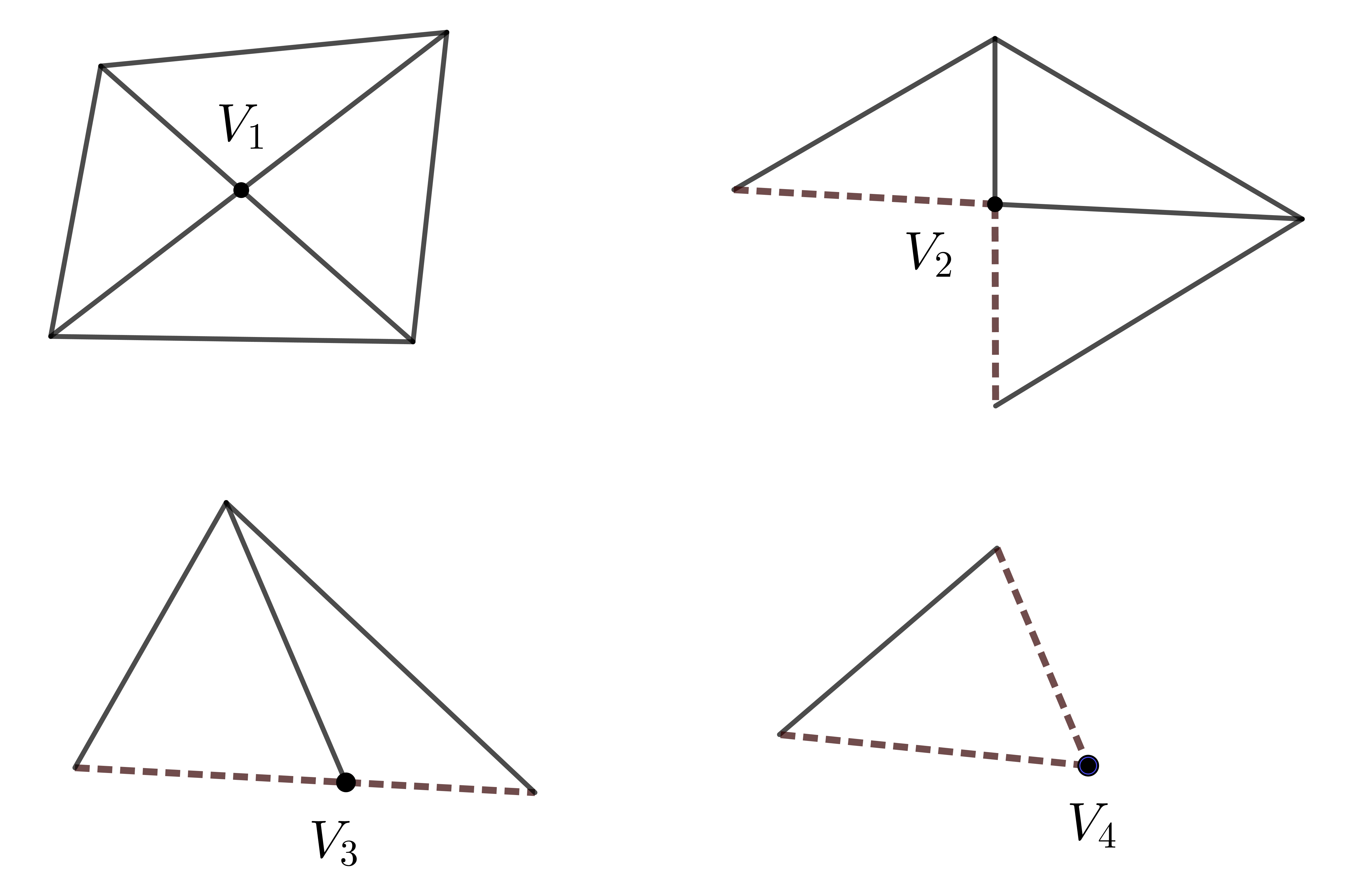
Figure 1: Four types of exactly singular vertices $\mathbf{V}_{1},\mathbf{V}_{2},\mathbf{V}_{3},\mathbf{V}_{4}$ (dashed edges belong to $\partial\Omega$.)

For each vertex $\mathbf{V}$, denote by $\Upsilon(\mathbf{V})$, the set of all sums of two adjacent angles of $\mathbf{V}$ in two back-to back triangles in $\mathcal{T}_{h}$. Then $\Upsilon(\mathbf{V})=\{\pi\}\mbox{ or }\emptyset$ if and only if $\mathbf{V}$ is singular. For examples, in Figure 1,

$$\Upsilon(\mathbf{V}_{1})=\Upsilon(\mathbf{V}_{2})=\Upsilon(\mathbf{V}_{3})=\{\pi\},\quad\Upsilon(\mathbf{V}_{4})=\emptyset.$$

Since $\{\mathcal{T}_{h}\}_{h>0}$ is regular, there exists $\vartheta>0$ such that

$$\vartheta=\inf\{\theta\ |\ \theta\mbox{ is an angle of a triangle }K\in\mathcal{T}_{h},h>0\}.$$

Set

$$\vartheta_{\sigma}=\min(\vartheta,\pi/6),$$ (1)

then $\vartheta_{\sigma}$ depends on the shape regularity parameter $\sigma$ of $\{\mathcal{T}_{h}\}_{h>0}$. From (1), we note that every angles $\theta$ of a triangle $K$ in $\mathcal{T}_{h}$ satisfies that

$$\vartheta_{\sigma}\leq\theta\leq\pi-2\vartheta_{\sigma}.$$ (2)

We will call a vertex $\mathbf{V}\in\mathcal{V}_{h}$ quasi singular if it is singular or nearly singular. For quantification, define a set

$$\mathcal{S}_{h}=\{\mathbf{V}\in\mathcal{V}_{h}\ :\ |\Theta-\pi|<\vartheta_{\sigma}\mbox{ for all }\Theta\in\Upsilon(\mathbf{V})\}.$$ (3)

Then, we call a vertex $\mathbf{V}$ quasi singular if $\mathbf{V}\in\SS_{h}$, otherwise regular. In Figure 2, examples of quasi but not exactly singular vertices are depicted. Interior quasi singular vertices are slight perturbations of exactly singular ones. It results in the following lemma:

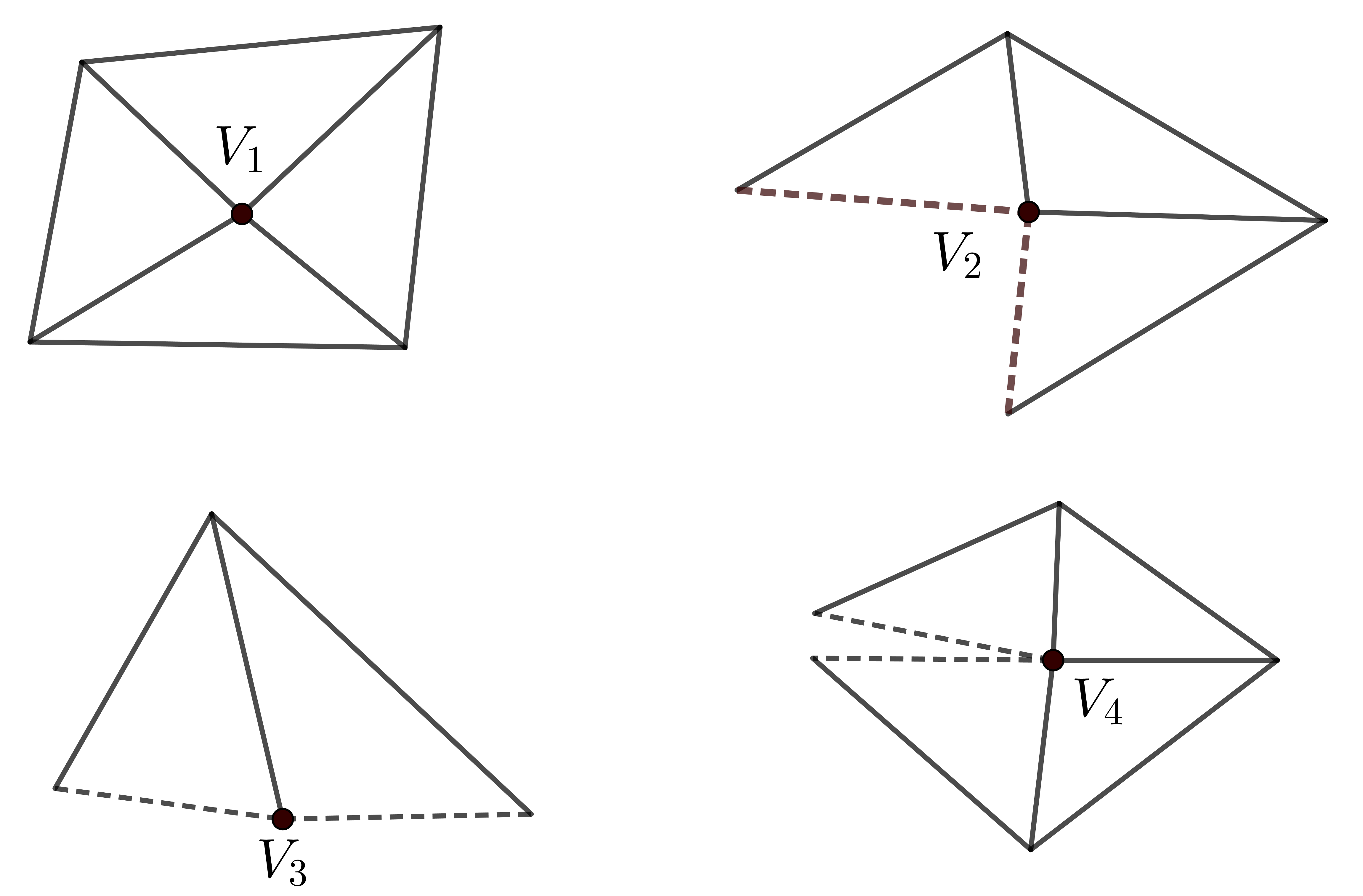
Figure 2: Quasi but not exactly singular vertices $\mathbf{V}_{1},\mathbf{V}_{2},\mathbf{V}_{3},\mathbf{V}_{4}$ (dashed edges belong to $\partial\Omega$.)

Lemma 2.1.

If $\mathbf{V}$ is an interior quasi singular vertex, then the number of all triangles sharing $\mathbf{V}$ is $4$.

Proof.

Let $N$ be the number of all triangles sharing $\mathbf{V}$ and $\theta_{1},\theta_{2},\cdots,\theta_{N}$ back-to-back angles of $\mathbf{V}$. Set

$$\Theta=\min\{\theta_{1}+\theta_{2},\theta_{2}+\theta_{3},\cdots,\theta_{N}+\theta_{1}\}.$$

Then,

$$N\Theta\leq 2\sum_{i=1}^{N}\theta_{i}=4\pi.$$ (4)

If $N\geq 5$, then (3) and (4) makes the following contradiction to $\vartheta_{\sigma}\leq\pi/6$ in (1):

$$\pi-\vartheta_{\sigma}<\Theta\leq\frac{4}{5}\pi.$$

If $N=3$, we have from (2),

$$\theta_{1}+\theta_{2}=2\pi-\theta_{3}\geq 2\pi-(\pi-2\vartheta_{\sigma})=\pi+2\vartheta_{\sigma}.$$

It contradicts to $\mathbf{V}\in\SS_{h}$. ∎

Each interior quasi singular vertex in $\SS_{h}$ is isolated from others in $\SS_{h}$ in the sense of the following lemma.

Lemma 2.2.

There is no interior edge connecting two quasi singular vertices in $\SS_{h}$.

Proof.

Let $E$ be an interior edge whose two endpoints $\mathbf{V}_{1},\mathbf{V}_{2}$ are quasi singular in $\SS_{h}$. Then, there exist two triangles sharing $E,\mathbf{V}_{1},\mathbf{V}_{2}$ as in Figure 3.

Consider the quadrilateral $Q$ whose vertices are $\mathbf{V}_{1},\mathbf{V}_{4},\mathbf{V}_{2},\mathbf{V}_{3}$ and one of its diagonals is $E$. Denote the angle of $\mathbf{V}_{i}$ in $Q$ by $\theta_{i}$, $i=1,2,3,4$. Then, from (2) and the definition of $\SS_{h}$, we have

$$\pi-\theta_{j}<\vartheta_{\sigma},\mbox{ if }j=1,2,\qquad\vartheta_{\sigma}\leq\theta_{j},\mbox{ if }j=3,4.$$

It meets with the following contradiction:

$$2\pi<\theta_{1}+\theta_{2}+\theta_{3}+\theta_{4}=2\pi.$$

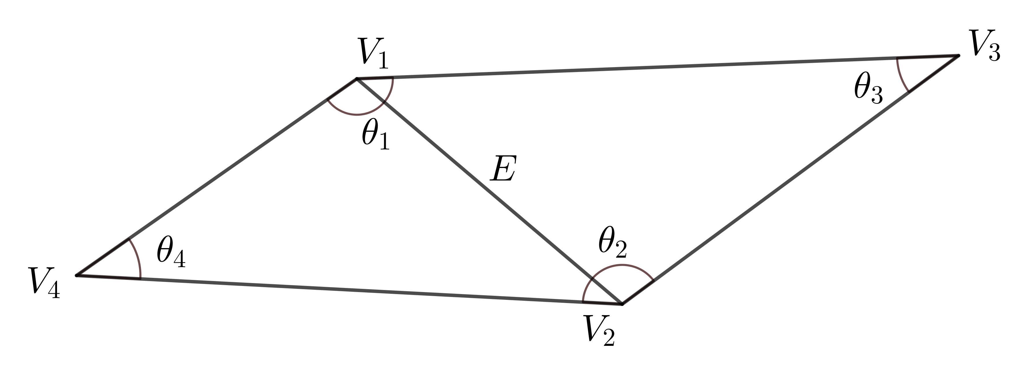
Figure 3: Two quasi singular vertices $\mathbf{V}_{1},\mathbf{V}_{2}$ form a quadrilateral with sharp angles $\theta_{3},\theta_{4}$

∎

3 Scott-Vogelius elements

Let’s define the discrete polynomial spaces $\mathcal{P}_{k,h}(\Omega)$ as

$$\mathcal{P}_{k,h}(\Omega)=\{v_{h}\in L^{2}(\Omega)\ :\ v_{h}|_{K}\in P^{k}\mbox{ for all triangles }K\in\mathcal{T}_{h}\},\quad k\geq 0.$$

Then the Scott-Vogelius finite element space is the pair of $X_{h}^{k},M_{h}^{k-1}$ such that

$$X_{h}^{k}={[\mathcal{P}_{k,h}(\Omega)\cap H_{0}^{1}(\Omega)]^{2}},\qquad M_{h}^{k-1}={\mathcal{P}_{k-1,h}(\Omega)\cap L_{0}^{2}(\Omega)},\quad k\geq 4,$$

where $L_{0}^{2}(\Omega)$ is the space of square integrable functions whose means vanish. In this paper, we deal with only the Scott-Vogelius finite element space of the lowest order:

$$X_{h}={[\mathcal{P}_{4,h}(\Omega)\cap H_{0}^{1}(\Omega)]^{2}},\qquad M_{h}={\mathcal{P}_{3,h}(\Omega)\cap L_{0}^{2}(\Omega)}).$$

The incompressible Stokes problem is to find $(\mathbf{u},p)\in[H_{0}^{1}(\Omega)]^{2}\times L_{0}^{2}(\Omega)$ such that

$$(\nabla\mathbf{u},\nabla\mathbf{v})+(p,\mathrm{div}\hskip 1.42262pt\mathbf{v})+(q,\mathrm{div}\hskip 1.42262pt\mathbf{u})=(\mathbf{f},\mathbf{v})\quad\mbox{ for all }(\mathbf{v},q)\in[H_{0}^{1}(\Omega)]^{2}\times L_{0}^{2}(\Omega),$$ (5)

for a given source function $\mathbf{f}\in[L_{0}^{2}(\Omega)]^{2}$. We will consider the discrete Stokes problem for (5) to find $(\mathbf{u}_{h},p_{h})\in X_{h}\times M_{h}$ such that

$$(\nabla\mathbf{u}_{h},\nabla\mathbf{v}_{h})+(p_{h},\mathrm{div}\hskip 1.42262pt\mathbf{v}_{h})+(q_{h},\mathrm{div}\hskip 1.42262pt\mathbf{u}_{h})=(\mathbf{f},\mathbf{v}_{h})\quad\mbox{ for all }(\mathbf{v}_{h},q_{h})\in X_{h}\times M_{h}.$$ (6)

3.1 Error in velocity

Let $M_{h}^{S}$ is the space of spurious pressures such that

$$M_{h}^{S}=\{s_{h}\in M_{h}\ |\ (s_{h},\mathrm{div}\hskip 1.42262pt\mathbf{v}_{h})=0\mbox{ for all }\mathbf{v}_{h}\in X_{h}\}.$$ (7)

Unfortunately, $M_{h}^{S}$ is not null, if $\mathcal{T}_{h}$ has an exact singular vertex as will be discussed in subsection 4.3 below. The discrete problem (6), however, has at least one solution, even if $M_{h}^{S}\neq\{0\}$.

Lemma 3.1.

There exists $(\mathbf{u}_{h},p_{h})\in X_{h}\times M_{h}$ satisfying (6). In addition, $\mathbf{u}_{h}$ is unique.

Proof.

Let $M_{h}=M_{h}^{S}\bigoplus\hat{M_{h}}$ for some subspace $\hat{M_{h}}$. Then there exists a unique $(\mathbf{u}_{h},\hat{p_{h}})\in X_{h}\times\hat{M_{h}}$ satisfying (6), since the discrete problem is not singular on $X_{h}\times\hat{M_{h}}$. ∎

Let $\Upsilon^{\prime}(\mathbf{V})=\Upsilon(\mathbf{V})\cup\{0\}$ and define a parameter $\Theta_{\min}$ of the triangulation $\mathcal{T}_{h}$ as

$$\Theta_{\min}=\min_{\mathbf{V}\in\mathcal{V}_{h}}\max_{\Theta\in\Upsilon^{\prime}(\mathbf{V})}|\sin\Theta|.$$

The following inf-sup condition is well known [6]:

$$\Theta_{\min}\beta\|q_{h}\|_{0}\leq\sup_{\mathbf{v}_{h}\in X_{h}\setminus\{0\}}\frac{(q_{h},\mathrm{div}\hskip 1.42262pt\mathbf{v}_{h})}{|\mathbf{v}_{h}|_{1}},\quad\forall q_{h}\in M_{h}.$$ (8)

If $\mathcal{T}_{h}$ has a quasi singular vertex in $\SS_{h}$, $\Theta_{\min}$ is zero or might be quite small. It could spoil the discrete pressure $p_{h}$ as in Figure 15. Although the inf-sup condition in (8) depends on $\Theta_{\min}$, the error in velocity is stable independently of $\Theta_{\min}$.

Throughout inequalities in the paper, a generic notation $C$ denotes a constant which depends only on $\Omega$ and the shape regularity parameter $\sigma$.

Theorem 3.2.

Let $(\mathbf{u},p)\in[H_{0}^{1}(\Omega)]^{2}\times L_{0}^{2}(\Omega)$ and $(\mathbf{u}_{h},p_{h})\in X_{h}\times M_{h}$ satisfy (5), (6), respectively. Then, if $\mathbf{u}\in[H^{5}(\Omega)]^{2}$, we have

$$|\mathbf{u}-\mathbf{u}_{h}|_{1}\leq Ch^{4}|\mathbf{u}|_{5}.$$

Proof.

Since $\mathrm{div}\hskip 1.42262pt\mathbf{u}=0$, there exists a stream function $\phi\in H^{6}(\Omega)$ of $\mathbf{u}$ which is constant on each component of $\partial\Omega$. Let $\phi_{h}$ be the projection of $\phi$ into the space of $C^{1}$-Argyris triangle elements which are locally $P^{5}$ [2, 3, 4]. Then, $\nabla\phi_{h}$ is continuous in $\Omega$ and vanishes on $\partial\Omega$ and $\phi_{h}$ satisfies that

$$|\phi-\phi_{h}|_{2}\leq Ch^{4}|\phi|_{6}.$$

Thus, if we define $\Pi_{h}\mathbf{u}=\mathbf{curl}\hskip 1.42262pt\phi_{h}$, we have $\Pi_{h}\mathbf{u}\in X_{h}$ and

$$|\mathbf{u}-\Pi_{h}\mathbf{u}|_{1}\leq Ch^{4}|\mathbf{u}|_{5}.$$ (9)

Let

$$V_{h}=\{\mathbf{v}_{h}\in X_{h}\ |\ (q_{h},\mathrm{div}\hskip 1.42262pt\mathbf{v}_{h})=0\mbox{ for all }q_{h}\in M_{h}\}.$$

Note $\mathrm{div}\hskip 1.42262pt\mathbf{v}_{h}=0$, if $\mathbf{v}_{h}\in V_{h}$. Then, from (5), (6), $\mathbf{u}$ and $\mathbf{u}_{h}$ satisfy that

$$(\nabla\mathbf{u}-\nabla\Pi_{h}\mathbf{u},\nabla\mathbf{v}_{h})=(\nabla\mathbf{u}_{h}-\nabla\Pi_{h}\mathbf{u},\nabla\mathbf{v}_{h})\mbox{ for all }\mathbf{v}_{h}\in V_{h}.$$ (10)

Since $\mathbf{u}_{h},\Pi_{h}\mathbf{u}_{h}\in V_{h}$, we have, for $\mathbf{v}_{h}=\mathbf{u}_{h}-\Pi_{h}\mathbf{u}\in V_{h}$ in (10),

$$|\mathbf{u}_{h}-\Pi_{h}\mathbf{u}|_{1}^{2}\leq|\mathbf{u}-\Pi_{h}\mathbf{u}|_{1}|\mathbf{u}_{h}-\Pi_{h}\mathbf{u}|_{1}.$$

It completes the proof with (9). ∎

4 Spurious pressure

4.1 Sting functions

Let $K$ be a triangle in $\mathcal{T}_{h}$ which has an edge $E$ and its opposite vertex $\mathbf{V}$ as in Figure 8-(b). Denote by $\lambda(\mathbf{x})$, a barycentric coordinate of $\mathbf{x}$ vanishing on $E$ such that

$$\lambda(\mathbf{x})=(-\mathbf{n})\cdot(\mathbf{x}-\mathbf{M}),$$

where $\mathbf{n}$ is the unit outward normal vector of $K$ on $E$ and $\mathbf{M}$ is the center of $E$.

With a specific function $\mathpzc{e}$:

$$\mathpzc{e}(t)=\frac{1}{10}(56t^{3}-63t^{2}+18t-1),$$ (11)

define a cubic polynomial $s_{E\mathbf{V}}\in P^{3}(K)$ determined by the edge $E$ and its opposite vertex $\mathbf{V}$:

$$s_{E\mathbf{V}}(\mathbf{x})=\mathpzc{e}\Big{(}\frac{\lambda(\mathbf{x})}{H}\Big{)},$$ (12)

where $H$ is the distance between $E$ and $\mathbf{V}$. A graph of $s_{E\mathbf{V}}$ is depicted in Figure 4 in the reference triangle $\widehat{K}$. We would name $s_{E\mathbf{V}}$ a sting function after its look.

In the remaining of the paper, a local function such as $s_{E\mathbf{V}}$ defined on $K$ is identified with its trivial extension on $\Omega$ vanishing outside $K$. We also use a notation $C_{\sigma}$ for a generic constant which depends only on the shape regularity parameter $\sigma$.

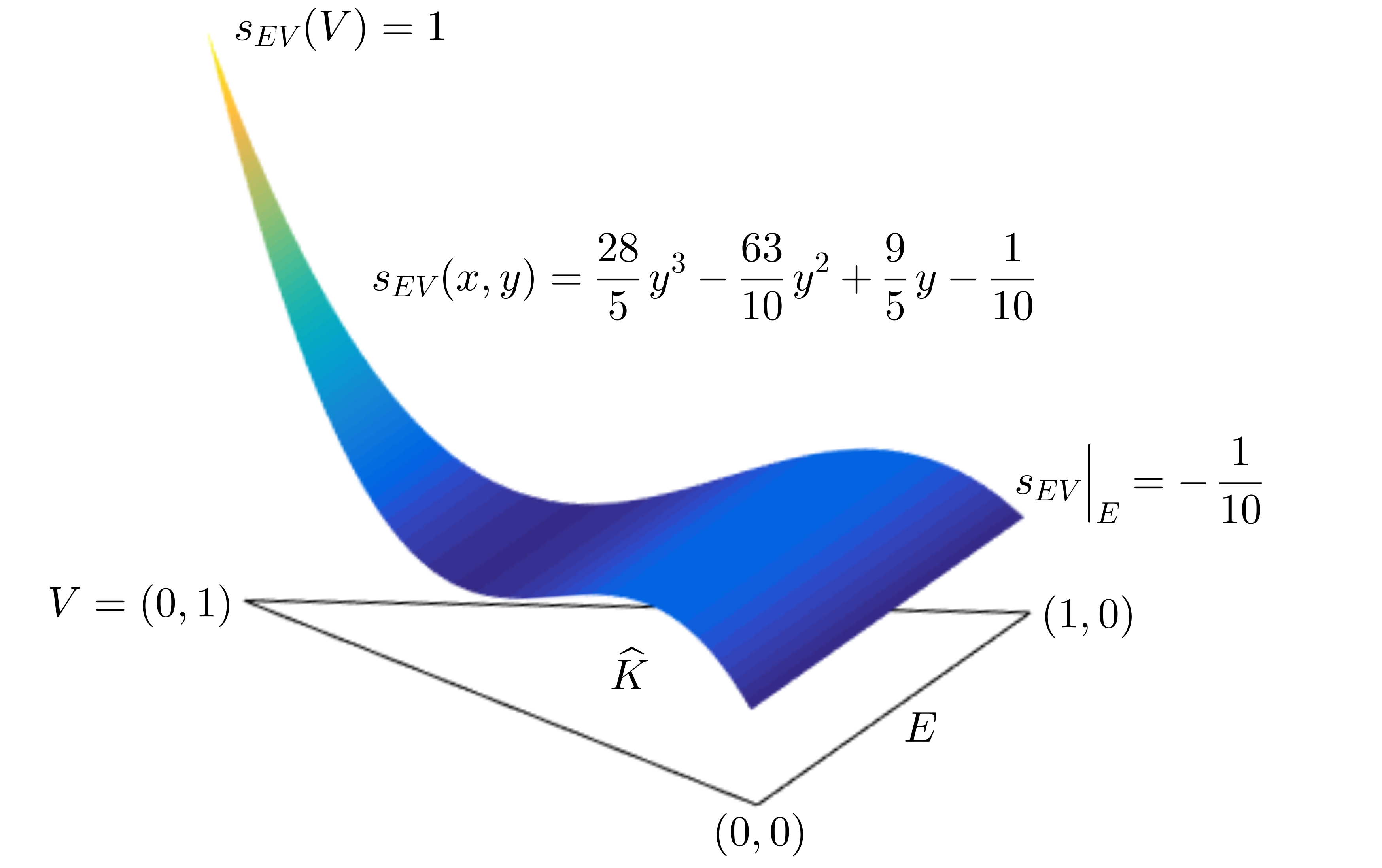
Figure 4: A sting function $s_{E\mathbf{V}}\in P^{3}$ over $\widehat{K}$

4.2 Quadrature rules

The choice of $\mathpzc{e}$ in (11) makes the sting function $s_{E\mathbf{V}}$ satisfy the following two quadrature rules which play key roles in our error analysis for pressure.

Lemma 4.1.

Let $E$ be an edge of a triangle $K$ and $\mathbf{V}$ its opposite vertex. Then, for each polynomial $q\in P^{3}(K)$, we have

$$\int_{K}s_{E\mathbf{V}}\ q\ dA=\frac{|K|}{100}q(\mathbf{V}).$$ (13)

Proof.

In the reference triangle $\widehat{K}$ with its vertices $(0,0),(1,0),(0,1)$, let $E=\{(x,0)\hskip 1.0pt:\hskip 1.0pt0\leq x\leq 1\}$ with its opposite vertex $\mathbf{V}=(0,1)$. By an affine map $\widehat{K}\rightarrow K$, sting functions on $K$ are pulled back to $s_{E\mathbf{V}}$ on $\widehat{K}$. Thus, it is sufficient to prove (13) for $s_{E\mathbf{V}}$ and a cubic polynomial $q$ in $\widehat{K}$.

By definition in (12), we have

$$s_{E\mathbf{V}}(x,y)=\frac{1}{10}(56y^{3}-63y^{2}+18y-1).$$ (14)

The graph of $s_{E\mathbf{V}}$ is depicted in Figure 4.

By simple calculation, we have

$$\int_{0}^{1}(56s^{3}-105s^{2}+60s-10)s^{k}\ ds=\left\{\begin{array}[]{cl}\displaystyle\frac{-1}{20},&\mbox{ if }k=1,\\ 0,&\mbox{ if }k=2,3,4.\end{array}\right.$$ (15)

We also note

$$56t^{3}-63t^{2}+18t-1=-56(1-t)^{3}+105(1-t)^{2}-60(1-t)+10.$$ (16)

Let $q=(1-y)^{m}x^{n}$ be a polynomial for nonnegative integers $m,n$ such that $m+n\leq 3$. From (14)-(16), we can expand that

$$\begin{array}[]{l}\displaystyle\int_{\widehat{K}}s_{E\mathbf{V}}(x,y)q(x,y)\ dA=\frac{1}{10}\int_{0}^{1}(56y^{3}-63y^{2}+18y-1)(1-y)^{m}\int_{0}^{1-y}x^{n}\ dxdy\\ \qquad=\displaystyle\frac{-1}{10(n+1)}\int_{0}^{1}\big{(}56(1-y)^{3}-105(1-y)^{2}+60(1-y)-10\big{)}(1-y)^{m+n+1}\ dy\\ \qquad=\displaystyle\frac{-1}{10(n+1)}\int_{0}^{1}\big{(}56s^{3}-105s^{2}+60s-10\big{)}s^{m+n+1}\ ds=\displaystyle\frac{1}{200}q(0,1)=\displaystyle\frac{|\widehat{K}|}{100}q(\mathbf{V}).\end{array}$$

∎

Figure 5: Counterclockwisely numbered unit vectors $\boldsymbol{\tau}_{1},\boldsymbol{\tau}_{2}$ directed to other vertices from $\mathbf{V}$

Lemma 4.2.

Let $E$ be an edge of a triangle $K$ and $\mathbf{V}$ its opposite vertex. Denote by $\boldsymbol{\tau}_{1},\boldsymbol{\tau}_{2}$, the counterclockwisely numbered unit vectors directed to other vertices $\mathbf{V}_{1},\mathbf{V}_{2}$ from $\mathbf{V}$ as in Figure 5. Then for all $\mathbf{v}_{h}\in X_{h}$, we have

$$(s_{E\mathbf{V}},\mathrm{div}\hskip 1.42262pt\mathbf{v}_{h})_{K}=\frac{|E_{1}||E_{2}|}{200}\Big{(}\frac{\partial\mathbf{v}_{h}}{\partial\boldsymbol{\tau}_{2}}(\mathbf{V})\cdot\boldsymbol{\tau}_{1}^{\perp}-\frac{\partial\mathbf{v}_{h}}{\partial\boldsymbol{\tau}_{1}}(\mathbf{V})\cdot\boldsymbol{\tau}_{2}^{\perp}\Big{)},$$

where $E_{1},E_{2}$ are the edges sharing $\mathbf{V}$ and $\boldsymbol{\tau}_{i}^{\perp}$ is the 90-degree counterclockwise rotation of $\boldsymbol{\tau}_{i},i=1,2$.

Proof.

For $\mathbf{v}_{h}=(v_{1},v_{2})$, we write $\displaystyle\frac{\partial\mathbf{v}_{h}}{\partial\boldsymbol{\tau}_{1}},\frac{\partial\mathbf{v}_{h}}{\partial\boldsymbol{\tau}_{2}}$ at $\mathbf{V}$ in the matrix form:

$$\left(\begin{array}[]{c}\nabla v_{1}(\mathbf{V})^{t}\\ \nabla v_{2}(\mathbf{V})^{t}\end{array}\right)(\boldsymbol{\tau}_{1}\ \boldsymbol{\tau}_{2})=\Big{(}\frac{\partial\mathbf{v}_{h}}{\partial\boldsymbol{\tau}_{1}}(\mathbf{V})\ \frac{\partial\mathbf{v}_{h}}{\partial\boldsymbol{\tau}_{2}}(\mathbf{V})\Big{)},$$

where all vectors are presented in column forms. Then we expand that

$$\begin{array}[]{ll}\mathrm{div}\hskip 1.42262pt\mathbf{v}_{h}(\mathbf{V})&=\mbox{trace}\left(\begin{array}[]{c}\nabla v_{1}(\mathbf{V})^{t}\\ \nabla v_{2}(\mathbf{V})^{t}\end{array}\right)=\mbox{trace}\Big{(}(\boldsymbol{\tau}_{1}\ \boldsymbol{\tau}_{2})^{-1}\Big{(}\displaystyle\frac{\partial\mathbf{v}_{h}}{\partial\boldsymbol{\tau}_{1}}(\mathbf{V})\ \frac{\partial\mathbf{v}_{h}}{\partial\boldsymbol{\tau}_{2}}(\mathbf{V})\Big{)}\Big{)}\\ &=\displaystyle\frac{1}{\sin\theta}\mbox{trace}\left(\left(\begin{array}[]{c}-(\boldsymbol{\tau}_{2}^{\perp})^{t}\\ (\boldsymbol{\tau}_{1}^{\perp})^{t}\end{array}\right)\Big{(}\frac{\partial\mathbf{v}_{h}}{\partial\boldsymbol{\tau}_{1}}(\mathbf{V})\ \frac{\partial\mathbf{v}_{h}}{\partial\boldsymbol{\tau}_{2}}(\mathbf{V})\Big{)}\right)\\ &=\displaystyle\frac{1}{\sin\theta}\Big{(}\boldsymbol{\tau}_{1}^{\perp}\cdot\frac{\partial\mathbf{v}_{h}}{\partial\boldsymbol{\tau}_{2}}(\mathbf{V})-\boldsymbol{\tau}_{2}^{\perp}\cdot\frac{\partial\mathbf{v}_{h}}{\partial\boldsymbol{\tau}_{1}}(\mathbf{V})\Big{)},\end{array}$$ (17)

where $\theta$ is the angle between $\boldsymbol{\tau}_{1}$ and $\boldsymbol{\tau}_{2}$. Since $|K|=\frac{1}{2}|E_{1}||E_{2}|\sin\theta$, we obtain (4.2) with the aid of (17) and Lemma 4.1. ∎

4.3 Spurious pressure

If $\mathcal{T}_{h}$ has an exact singular vertex, a spurious pressure in $M_{h}^{S}$ defined in (7) appears. For a simple example, let $\mathbf{V}$ be a boundary singular vertex which meets only one triangle $K$ in $\mathcal{T}_{h}$ and has its opposite edge $E$ as $\mathbf{V}_{4}$ in Figure 1. Then, by Lemma 4.1, we obtain

$$(s_{E\mathbf{V}},\mathrm{div}\hskip 1.42262pt\mathbf{v}_{h})_{K}=\frac{|K|}{100}\mathrm{div}\hskip 1.42262pt\mathbf{v}_{h}(\mathbf{V})=0\quad\mbox{ for all }\mathbf{v}_{h}\in X_{h},$$

since $\nabla\mathbf{v}_{h}$ vanishes at $\mathbf{V}$. Thus, $s_{E\mathbf{V}}-c$ is a spurious pressure in $M_{h}^{S}$ for a constant function $c$ on $\Omega$ such that $s_{E\mathbf{V}}-c\in L_{0}^{2}(\Omega)$.

For an another example, let $\mathbf{V}$ be an interior singular vertex which meets with 4 triangles $K_{1},K_{2},K_{3},K_{4}$ counterclockwisely numbered as in figure 6. The vertex $\mathbf{V}$ has 4 opposite edges $E_{i}\subset K_{i},i=1,2,3,4$. Denote by $\boldsymbol{\tau}_{1},\boldsymbol{\tau}_{2}$, the counterclockwisely numbered unit vectors at $\mathbf{V}$ directed other vertices in $K_{1}$ and by $\ell_{1},\ell_{2},\ell_{3},\ell_{4}$, the lengths of edges corresponding to $\boldsymbol{\tau}_{1},\boldsymbol{\tau}_{2},-\boldsymbol{\tau}_{1},-\boldsymbol{\tau}_{2}$, respectively.

Now, we calculate the followings by Lemma 4.2:

$$\begin{array}[]{lcl}(s_{E_{1}\mathbf{V}},\mathrm{div}\hskip 1.42262pt\mathbf{v}_{h})_{K_{1}}&=&\displaystyle\frac{\ell_{1}\ell_{2}}{200}\Big{(}\frac{\partial\mathbf{v}_{h}}{\partial\boldsymbol{\tau}_{2}}(\mathbf{V})\boldsymbol{\tau}_{1}^{\perp}-\frac{\partial\mathbf{v}_{h}}{\partial\boldsymbol{\tau}_{1}}(\mathbf{V})\boldsymbol{\tau}_{2}^{\perp}\Big{)},\\ (s_{E_{2}\mathbf{V}},\mathrm{div}\hskip 1.42262pt\mathbf{v}_{h})_{K_{2}}&=&\displaystyle\frac{\ell_{2}\ell_{3}}{200}\Big{(}\frac{\partial\mathbf{v}_{h}}{\partial(-\boldsymbol{\tau}_{1})}(\mathbf{V})\boldsymbol{\tau}_{2}^{\perp}-\frac{\partial\mathbf{v}_{h}}{\partial\boldsymbol{\tau}_{2}}(\mathbf{V})(-\boldsymbol{\tau}_{1})^{\perp}\Big{)},\\ (s_{E_{3}\mathbf{V}},\mathrm{div}\hskip 1.42262pt\mathbf{v}_{h})_{K_{3}}&=&\displaystyle\frac{\ell_{3}\ell_{4}}{200}\Big{(}\frac{\partial\mathbf{v}_{h}}{\partial(-\boldsymbol{\tau}_{2})}(\mathbf{V})(-\boldsymbol{\tau}_{1})^{\perp}-\frac{\partial\mathbf{v}_{h}}{\partial(-\boldsymbol{\tau}_{1})}(\mathbf{V})(-\boldsymbol{\tau}_{2})^{\perp}\Big{)},\\ (s_{E_{4}\mathbf{V}},\mathrm{div}\hskip 1.42262pt\mathbf{v}_{h})_{K_{4}}&=&\displaystyle\frac{\ell_{4}\ell_{1}}{200}\Big{(}\frac{\partial\mathbf{v}_{h}}{\partial\boldsymbol{\tau}_{1}}(\mathbf{V})(-\boldsymbol{\tau}_{2})^{\perp}-\frac{\partial\mathbf{v}_{h}}{\partial(-\boldsymbol{\tau}_{2})}(\mathbf{V})\boldsymbol{\tau}_{1}^{\perp}\Big{)}.\end{array}$$ (18)

Let $q_{h}\in M_{h}$ be an alternating sum of $s_{E_{i}\mathbf{V}},i=1,2,3,4$ such that

$$q_{h}=\frac{1}{\ell_{1}\ell_{2}}s_{E_{1}\mathbf{V}}-\frac{1}{\ell_{2}\ell_{3}}s_{E_{2}\mathbf{V}}+\frac{1}{\ell_{3}\ell_{4}}s_{E_{3}\mathbf{V}}-\frac{1}{\ell_{4}\ell_{1}}s_{E_{4}\mathbf{V}}.$$ (19)

Then, since $\mathbf{v}_{h}$ is continuous on edges, we have from (18),

$$(q_{h},\mathrm{div}\hskip 1.42262pt\mathbf{v}_{h})=0\quad\mbox{ for all }\mathbf{v}_{h}\in X_{h}.$$

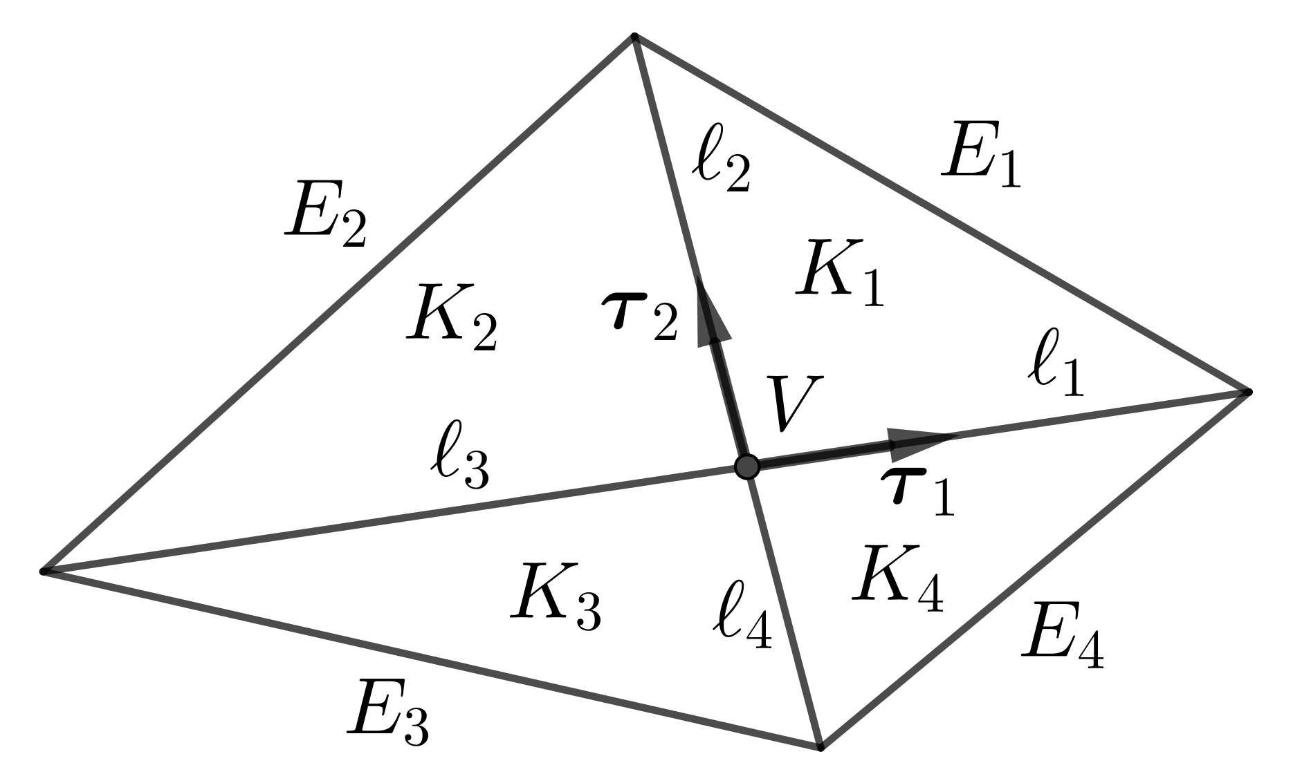
Figure 6: Interior exact singular vertex $\mathbf{V}$ causing a spurious pressure

5 A basis of $P^{3}$ over $K$

We will suggest a new basis of $P^{3}$ over a triangle $K$ which includes sting functions $s_{E\mathbf{V}}$.

5.1 16-point Lyness quadrature rule

The following 16-point Lyness quadrature rule [7] is exact over a triangle $K$ for any polynomial $p$ of degree up to 6:

$$\int_{{K}}p(x,y)\ dxdy=|K|\sum_{i=1}^{16}p(\mathbf{x}_{i})w_{i}.$$ (20)

The 16 quadrature points in (20) include the gravity center $\mathbf{G}$ of $K$ and the center $\mathbf{G}_{i}$ of the segment connecting the vertex $\mathbf{V}_{i}$ and the midpoint $\mathbf{M}_{i}$ of the opposite edge of $\mathbf{V}_{i}$, $i=1,2,3$ as in Figure 7. The other 12 points lie on the boundary of $K$.

Figure 7: 16 Lyness quadrature points, $\mathbf{G}_{i}$ is the center of $\overline{\mathbf{V}_{i}\mathbf{M}_{i}}\ i=1,2,3$

In the reference triangle $\hat{K}$ with vertices $(0,0),(1,0),(0,1)$, the 16 quadrature points and their corresponding weights are listed:

$$\begin{array}[]{ccl}\{\mathbf{x}_{i}\}_{1}^{3}&=&\{(0,0),(1,0),(0,1)\},\quad\{w_{i}\}_{1}^{3}=\{-5/252\},\\ \{\mathbf{x}_{i}\}_{4}^{9}&=&\{(0,a),(0,b),(a,0),(b,0),(a,b),(b,a)\},\quad\{w_{i}\}_{4}^{9}=\{3/70\},\\ \{\mathbf{x}_{i}\}_{10}^{12}&=&\{(0,1/2),(1/2,0),(1/2,1/2)\},\quad\{w_{i}\}_{10}^{12}=\{17/315\},\\ \{\mathbf{x}_{i}\}_{13}^{15}&=&\{(1/4,1/4),(1/4,1/2),(1/2,1/4)\},\quad\{w_{i}\}_{13}^{15}=\{128/315\},\\ \mathbf{x}_{16}&=&(1/3,1/3),\quad w_{16}=-81/140,\end{array}$$ (21)

where $a=(3-\sqrt{6})/6,\ b=1-a$.

5.2 Basis functions with interior Lyness points

Let $\mathbf{V}$ be a vertex of a triangle $K$ and $\mathbf{G}$ the gravity center of $K$. Denote by $\mathbf{i}_{\mathbf{V}}$, the unit vector from $\mathbf{V}$ to $\mathbf{G}$ as in Figure 8-(a), that is

$$\mathbf{i}_{\mathbf{V}}=\overrightarrow{\mathbf{V}\mathbf{G}}\Big{/}|\overrightarrow{\mathbf{V}\mathbf{G}}|,$$

and by ${\mathbf{i}_{\mathbf{V}}}^{\perp}$, the 90-degree counterclockwise rotation of $\mathbf{i}_{\mathbf{V}}$, and by $\mu$, a linear function which vanishes at the line passing $\mathbf{V},\mathbf{G}$ such that

$$\mu(\mathbf{x})={\mathbf{i}_{\mathbf{V}}}^{\perp}\cdot(\mathbf{x}-\mathbf{G}),$$ (22)

lastly, by $d$, the common distance from two other vertices of $K$ to the line $\mu(\mathbf{x})=0$ as in Figure 8-(a).

(a) $\mu(\mathbf{x})={\mathbf{i}_{\mathbf{V}}}^{\perp}\cdot(\mathbf{x}-\mathbf{G}),\ g_{\mathbf{V}}^{\pm}=\mu^{\pm}\Big{(}\displaystyle\frac{\mu}{d}\Big{)}$

(b) $\lambda(\mathbf{x})={-\mathbf{n}}\cdot(\mathbf{x}-\mathbf{M}),\ s_{E\mathbf{V}}=\mathpzc{e}\Big{(}\displaystyle\frac{\lambda}{H}\Big{)}$

Figure 8: Definition of three basis cubic polynomials over $K$: $g_{\mathbf{V}}^{+},\ g_{\mathbf{V}}^{-},\ s_{E\mathbf{V}}$

Define two basis cubic polynomial $g_{\mathbf{V}}^{+},g_{\mathbf{V}}^{-}\in P^{3}(K)$ determined by $\mathbf{V},\mathbf{G}$:

$$g_{\mathbf{V}}^{+}(\mathbf{x})=\iota^{+}\Big{(}\frac{\mu(\mathbf{x})}{d}\Big{)},\quad g_{\mathbf{V}}^{-}(\mathbf{x})=\iota^{-}\Big{(}\frac{\mu(\mathbf{x})}{d}\Big{)},$$ (23)

with two auxiliary cubic functions $\iota^{+},\iota^{-}$:

$$\iota^{+}(t)=8t^{3}+3t^{2},\quad\iota^{-}(t)=8t^{3}-3t^{2}.$$

We have chosen $\iota^{\pm}$ so that $\nabla g^{\pm}_{\mathbf{V}}$ vanishes at 3 points among 4 interior Lyness points $\mathbf{G},\mathbf{G}_{1},\mathbf{G}_{2},\mathbf{G}_{3}$ of $K$ as in the following lemma.

Lemma 5.1.

Let $\mathbf{V}$ be a vertex of a triangle $K$ and $\mathbf{P}$ be among four 16-Lyness quadrature points inside $K$. Then, we have

$$\nabla g_{\mathbf{V}}^{+}(\mathbf{P})=\left\{\ \begin{array}[]{cl}\displaystyle\frac{3}{d}{\mathbf{i}_{\mathbf{V}}}^{\perp}&\mbox{ if }\mu(\mathbf{P})>0,\\ 0&\mbox{ otherwise },\end{array}\right.\qquad\nabla g_{\mathbf{V}}^{-}(\mathbf{P})=\left\{\ \begin{array}[]{cl}\displaystyle\frac{3}{d}{\mathbf{i}_{\mathbf{V}}}^{\perp}&\mbox{ if }\mu(\mathbf{P})<0,\\ 0&\mbox{ otherwise }.\end{array}\right.$$ (24)

Proof.

Let $\mathbf{V}^{+},\mathbf{V}^{-}$ be two vertices of triangle $K$ other than $\mathbf{V}$ such that

$$\mu(\mathbf{V}^{+})>0,\quad\mu(\mathbf{V}^{-})<0.$$

The four 16-Lyness quadrature points inside $K$ are the gravity center $\mathbf{G}$ and

$$\mathbf{G}_{0}=\frac{1}{2}\mathbf{V}+\frac{1}{4}\mathbf{V}^{+}+\frac{1}{4}\mathbf{V}^{-},\quad\mathbf{G}^{+}=\frac{1}{4}\mathbf{V}+\frac{1}{2}\mathbf{V}^{+}+\frac{1}{4}\mathbf{V}^{-},\quad\mathbf{G}^{-}=\frac{1}{4}\mathbf{V}+\frac{1}{4}\mathbf{V}^{+}+\frac{1}{2}\mathbf{V}^{-}.$$

The two points $\mathbf{G},\mathbf{G}_{0}$ lie on the line $l=\{\mathbf{x}:\mu(\mathbf{x})=0\}$ and we simply calculate the common distance between $l$ and $\mathbf{G}^{\pm}$ is a quarter of $d$ between $l$ and $\mathbf{V}^{\pm}$. Thus we have

$$\mu(\mathbf{G})=\mu(\mathbf{G}_{0})=0,\quad\mu(\mathbf{G}^{+})=\frac{d}{4},\quad\mu(\mathbf{G}^{-})=-\frac{d}{4}.$$ (25)

From the definition of $\mu,g_{\mathbf{V}}^{+}$ in (22),(23), we have

$$\nabla g_{\mathbf{V}}^{+}(\mathbf{x})=\frac{1}{d}{\iota^{+}}^{\prime}\Big{(}\frac{\mu(\mathbf{x})}{d}\Big{)}{\mathbf{i}_{\mathbf{V}}}^{\perp}.$$ (26)

We prove (24) for $\nabla g_{\mathbf{V}}^{+}$ by (25), (26), since ${\iota^{+}}^{\prime}(0)={\iota^{+}}^{\prime}(-1/4)=0,\ {\iota^{+}}^{\prime}(1/4)=3$. We can repeat the same argument for $\nabla g_{\mathbf{V}}^{-}$ in (24). ∎

Now, we form a new basis of $P^{3}$ over $K$ in the following lemma.

Lemma 5.2.

Let $K$ be a triangle with vertices $\mathbf{V}_{1},\mathbf{V}_{2},\mathbf{V}_{3}$ and their respective opposite edges $E_{1},E_{2},E_{3}$. Then, we have

$$P^{3}\ =\ <1,g_{\mathbf{V}_{1}}^{+},g_{\mathbf{V}_{1}}^{-},g_{\mathbf{V}_{2}}^{+},g_{\mathbf{V}_{2}}^{-},g_{\mathbf{V}_{3}}^{+},g_{\mathbf{V}_{3}}^{-},s_{E_{1}\mathbf{V}1},s_{E_{2}\mathbf{V}2},s_{E_{3}\mathbf{V}3}>.$$ (27)

Proof.

Assume a linear combination $q$ of 10 functions in (27) vanishes, that is,

$$q=c_{1}+c_{2}g_{\mathbf{V}_{1}}^{+}+c_{3}g_{\mathbf{V}_{1}}^{-}+c_{4}g_{\mathbf{V}_{2}}^{+}+c_{5}g_{\mathbf{V}_{2}}^{-}+c_{6}g_{\mathbf{V}_{3}}^{+}+c_{7}g_{\mathbf{V}_{3}}^{-}+c_{8}s_{E_{1}\mathbf{V}_{1}}+c_{9}s_{E_{2}\mathbf{V}_{2}}+c_{10}s_{E_{3}\mathbf{V}_{3}}=0,$$

for some scalars $c_{1},c_{2},\cdots,c_{10}$.

As in Figure 7, let $\mathbf{G}_{i}$ be the interior 16-Lyness points corresponding to $\mathbf{V}_{i}$, $i=1,2,3$. We can choose a quartic polynomial $v$ vanishing on $\partial K$ and satisfying

$$v(\mathbf{G}_{1})=v(\mathbf{G}_{2})=0,\quad v(\mathbf{G}_{3})=1.$$

For two scalars $\alpha,\beta$, define

$$\mathbf{v}=(\alpha,\beta)v.$$

We note from the quadrature rule in Lemma 4.1,

$$(s_{E_{i}\mathbf{V}_{i}},\mathrm{div}\hskip 1.42262pt\mathbf{v})=0,\quad i=1,2,3.$$ (28)

Thus, by 16-Lyness quadrature rule in (20), (21) and the property of $\nabla g_{\mathbf{V}_{i}}^{\pm},i=1,2,3$ in Lemma 5.1, we expand

$$\begin{array}[]{lcl}0&=&(q,\mathrm{div}\hskip 1.42262pt\mathbf{v})=-(\nabla q,\mathbf{v})=-\nabla(c_{2}g_{\mathbf{V}_{1}}^{+}+c_{5}g_{\mathbf{V}_{2}}^{-})(\mathbf{G}_{3})\cdot\mathbf{v}(\mathbf{G}_{3})w_{15}|K|\\ &=&(c_{2}\gamma_{1}{\mathbf{i}_{\mathbf{V}_{1}}}^{\perp}+c_{5}\gamma_{2}{\mathbf{i}_{\mathbf{V}_{2}}}^{\perp})\cdot(\alpha,\beta)w_{15}|K|,\end{array}$$ (29)

for some nonzero scalars $\gamma_{1},\gamma_{2}$.

If we choose $(\alpha,\beta)={\mathbf{i}_{\mathbf{V}_{2}}}$ in (29), we conclude $c_{2}=0$ and sequentially $c_{5}=0$, since $\mathbf{i}_{\mathbf{V}_{1}},\mathbf{i}_{\mathbf{V}_{2}}$ are not parallel. By similar argument, we have $c_{3}=c_{4}=c_{6}=c_{7}=0$.

Now choose a cubic polynomial $p$ such that its mean over $K$ vanishes and

$$p(\mathbf{V}_{1})=1,\quad p(\mathbf{V}_{2})=p(\mathbf{V}_{3})=0.$$

Then, by quadrature rule in Lemma 4.1, we have

$$0=(q,p)=(c_{8}s_{E_{1}\mathbf{V}_{1}},p)=c_{8}\frac{|K|}{100}p(\mathbf{V}_{1}).$$

Thus, $c_{8}=0$ and similarly, $c_{9}=c_{10}=0$. It completes the proof, since $\dim P^{3}=10$. ∎

6 Error in pressure

Let $(\mathbf{u},p)\in[H_{0}^{1}(\Omega)]^{2}\times L_{0}^{2}(\Omega)$ and $(\mathbf{u}_{h},p_{h})\in X_{h}\times M_{h}$ be the solutions for the continuous and discrete Stokes problems (5), (6), respectively. There exists a standard projection $\Pi_{h}p\in M_{h}$ of $p$ which is continuous in $\Omega$. Denoting the error in pressure by

$$e_{h}=p_{h}-\Pi_{h}p,$$ (30)

we will analyze that $e_{h}$ is stable except the spurious component of $e_{h}$ caused by quasi singular vertices.

By Theorem 3.2, we note that, if $\mathbf{u}\in[H^{5}(\Omega)]^{2}$ and $p\in H^{4}(\Omega)$, then

$$(e_{h},\mathrm{div}\hskip 1.42262pt\mathbf{v}_{h})\leq Ch^{4}(|\mathbf{u}|_{5}+|p|_{4})|\mathbf{v}_{h}|_{1}\quad\mbox{ for all }\mathbf{v}\in X_{h},$$ (31)

since $e_{h}$ satisfies

$$(e_{h},\mathrm{div}\hskip 1.42262pt\mathbf{v}_{h})=(\nabla\mathbf{u}-\nabla\mathbf{u}_{h},\nabla\mathbf{v}_{h})+(p-\Pi_{h}p,\mathrm{div}\hskip 1.42262pt\mathbf{v}_{h})\quad\mbox{ for all }\mathbf{v}\in X_{h}.$$ (32)

We will split $e_{h}$ into the interior error $e_{h}^{G}$ and sting error $e_{h}^{S}$:

$$e_{h}=e_{h}^{G}+e_{h}^{S},$$ (33)

where

$$e_{h}^{G}\big{|}_{K}\in<1,g_{\mathbf{V}_{1}}^{+},g_{\mathbf{V}_{1}}^{-},g_{\mathbf{V}_{2}}^{+},g_{\mathbf{V}_{2}}^{-},g_{\mathbf{V}_{3}}^{+},g_{\mathbf{V}_{3}}^{-}>,\quad e_{h}^{S}\big{|}_{K}\in<s_{E_{1}\mathbf{V}_{1}},s_{E_{2}\mathbf{V}_{2}},s_{E_{3}\mathbf{V}_{3}}>,$$

for each $K\in\mathcal{T}_{h}$ with vertices $\mathbf{V}_{1},\mathbf{V}_{2},\mathbf{V}_{3}$ and their respective opposite edges $E_{1},E_{2},E_{3}$.

For each vertex $\mathbf{V}$, let $\mathcal{E}_{\mathbf{V}}$ be a set of all opposite edges of $\mathbf{V}$. Then, we can cluster the sting error $e_{h}^{S}$ by vertices as

$$e_{h}^{S}=\sum_{\mathbf{V}\in\mathcal{V}_{h}}e_{h}^{\mathbf{V}},$$ (34)

where

$$e_{h}^{\mathbf{V}}\in<s_{E_{1}\mathbf{V}},s_{E_{2}\mathbf{V}},\cdots,s_{E_{J}\mathbf{V}}>,$$

for all opposite edges $E_{j}\in\mathcal{E}_{\mathbf{V}},\ j=1,2,\cdots,J=\#\mathcal{E}_{\mathbf{V}}.$

In the remaining of this section, we will show the error $e_{h}$ is stable except the sting error $e_{h}^{\mathbf{V}}$ for quasi singular vertices $\mathbf{V}$.

6.1 Inequalities for $e_{h}^{\mathbf{V}}$ in back-to-back triangles

We first estimate $\nabla e_{h}^{G}$ by choosing a proper test function $\mathbf{v}_{h}\in X_{h}$ in (32).

Lemma 6.1.

Let $h$ be the diameter of a triangle $K$ in $\mathcal{T}_{h}$. Then we have

$$h\|\nabla e_{h}^{G}\|_{0,K}\leq C_{\sigma}(|\mathbf{u}-\mathbf{u}_{h}|_{1,K}+\|p-\Pi_{h}p\|_{0,K}).$$

Proof.

With the same notations in Lemma 5.2, we represent

$$e_{h}^{G}\big{|}_{K}=c_{1}+c_{2}g_{\mathbf{V}_{1}}^{+}+c_{3}g_{\mathbf{V}_{1}}^{-}+c_{4}g_{\mathbf{V}_{2}}^{+}+c_{5}g_{\mathbf{V}_{2}}^{-}+c_{6}g_{\mathbf{V}_{3}}^{+}+c_{7}g_{\mathbf{V}_{3}}^{-},$$

for some constants $c_{1},c_{2},\cdots,c_{7}$. Denote by $\mathbf{G}_{i}$, the interior 16-Lyness points corresponding to $\mathbf{V}_{i}$, $i=1,2,3$ as in Figure 7. Then, there exists a unique quartic function $v\in P^{4}$ vanishing on $\partial K$ and $v(\mathbf{G}_{1})=v(\mathbf{G}_{2})=0,v(\mathbf{G}_{3})=1$. We note that

$$|v|_{1,K}\leq C_{\sigma}\quad|g_{\mathbf{V}_{i}}^{\pm}|_{1,K}\leq C_{\sigma},\ i=1,2,3.$$ (35)

Choose a test function $\mathbf{v}_{h}\in X_{h}$ such that $\mathbf{v}_{h}|_{K}=v\mathbf{i}_{\mathbf{V}_{2}}$ and vanishes outside $K$. Then, we have from (28) and Lemma 4.1, 5.1,

$$(e_{h},\mathrm{div}\hskip 1.42262pt\mathbf{v}_{h})=(e_{h}^{G},\mathrm{div}\hskip 1.42262pt\mathbf{v}_{h})_{K}=(\nabla e_{h}^{G},\mathbf{v}_{h})_{K}=3c_{2}{\mathbf{i}_{\mathbf{V}_{1}}}^{\perp}\cdot\mathbf{i}_{\mathbf{V}_{2}}w_{15}|K|/d,$$ (36)

where $d$ is the distance from $\mathbf{V}_{2}$ to the line connecting $\mathbf{V}_{1}$ and the gravity center $\mathbf{G}$.

Now, by (32), (35), (36), we estimate

$$\|c_{2}\nabla g_{\mathbf{V}_{1}}^{+}\|_{0,K}\leq C_{\sigma}h^{-1}(|\mathbf{u}-\mathbf{u}_{h}|_{1,K}+\|p-\Pi_{h}p\|_{0,K}).$$

It completes the proof, by repeating the same arguments for $c_{3},c_{4},\cdots,c_{7}$. ∎

Let $K$ be a triangle in $\mathcal{T}_{h}$ and $E$ an edge of $K$ between two vertices $\mathbf{V}_{1},\mathbf{V}_{2}$ of $K$. Denote by $\boldsymbol{\tau}$, the unit tangent vector of $E$, that is,

$$\boldsymbol{\tau}=\overrightarrow{\mathbf{V}_{1}\mathbf{V}_{2}}\Big{/}|\overrightarrow{\mathbf{V}_{1}\mathbf{V}_{2}}|.$$

We need an elementary test function $v$ in the following lemma to estimate the sting error $e_{h}^{S}$.

Lemma 6.2.

There exists a quartic polynomial $v\in P^{4}$ such that $v$ vanishes on $\partial K\setminus E$ and

$$\int_{E}v\ ds=0,\quad\frac{\partial v}{\partial\boldsymbol{\tau}}(\mathbf{V}_{1})=1,\quad\frac{\partial v}{\partial\boldsymbol{\tau}}(\mathbf{V}_{2})=0,\quad|v|_{1,K}\leq C_{\sigma}|E|.$$ (37)

Proof.

In the reference triangle $\widehat{K}$ with vertices $(0,0),(1,0),(0,1)$, let

$$\widehat{E}=\{(x,0)\ :\ 0\leq x\leq 1\},\quad\widehat{\mathbf{V}}_{1}=(0,0),\quad\widehat{\mathbf{V}}_{2}=(1,0),\quad\widehat{\boldsymbol{\tau}}=(1,0).$$

Then a quartic polynomial $\widehat{v}=x(x+y-1)^{2}(-5/2x+1)$ satisfies

$$\int_{\widehat{E}}\widehat{v}\ ds=0,\quad\displaystyle\frac{\partial\widehat{v}}{\partial\widehat{\boldsymbol{\tau}}}(\widehat{\mathbf{V}}_{1})=1,\quad\displaystyle\frac{\partial\widehat{v}}{\partial\widehat{\boldsymbol{\tau}}}(\widehat{\mathbf{V}}_{2})=0.$$ (38)

Define $v=|E|\ \hskip 1.0pt\widehat{v}\circ F^{-1}$ for an affine map $F:\widehat{K}\longrightarrow K$ such that $F(\widehat{\mathbf{V}}_{i})=\mathbf{V}_{i},i=1,2$. Then, from the definition of $\widehat{v}$ and (38), $v$ vanishes on $\partial K\setminus E$ and satisfies (37). ∎

The sting error $e_{h}^{\mathbf{V}}$ has an interesting characteristic for each pair of two back-to-back triangles sharing $\mathbf{V}$ in the following lemma.

Lemma 6.3.

Let two triangles $K_{1},K_{2}$ share a vertex $\mathbf{V}$ and an edge $E$ as in Figure 9. Assume two scalars $\alpha_{1},\alpha_{2}$ make that

$$e_{h}^{\mathbf{V}}\big{|}_{K_{1}\cup K_{2}}=\alpha_{1}s_{E_{1}\mathbf{V}}+\alpha_{2}s_{E_{2}\mathbf{V}},$$

for two opposite edges $E_{1},E_{2}$ of $\mathbf{V}$ in $K_{1},K_{2}$, respectively. Then for any unit vector $\boldsymbol{\xi}$, we have

$$\left|(\alpha_{1}\overrightarrow{\mathbf{V}\mathbf{V}_{1}}-\alpha_{2}\overrightarrow{\mathbf{V}\mathbf{V}_{2}})\cdot\boldsymbol{\xi}\right|\leq C_{\sigma}(|\mathbf{u}-\mathbf{u}_{h}|_{1,K_{1}\cup K_{2}}+\|p-\Pi_{h}p\|_{0,K_{1}\cup K_{2}}),$$ (39)

where $\mathbf{V}_{1},\mathbf{V}_{2}$ are the respective opposite vertices of $E$ in $K_{1},K_{2}$.

Proof.

Let $\mathbf{V}_{0}$ be the vertex of $E$ other than $\mathbf{V}$ and $\boldsymbol{\tau}$ unit vector such that

$$\boldsymbol{\tau}=\overrightarrow{\mathbf{V}\mathbf{V}_{0}}\Big{/}|\overrightarrow{\mathbf{V}\mathbf{V}_{0}}|.$$

From Lemma 6.2, there exists a quartic function $v_{i}$ on $K_{i},i=1,2$ such that $v_{i}$ vanishes on $\partial K_{i}\setminus E$ and

$$\int_{E}v_{i}\ ds=0,\quad\frac{\partial v_{i}}{\partial\boldsymbol{\tau}}(\mathbf{V})=1,\quad\frac{\partial v_{i}}{\partial\boldsymbol{\tau}}(\mathbf{V}_{0})=0,\quad|v_{i}|_{1,K_{i}}\leq C_{\sigma}|E|.$$ (40)

We note $v_{1}$ and $v_{2}$ coincide on $E$, since quartic functions have 5 degrees of freedom on $E$.

Given unit vector $\boldsymbol{\xi}$, denote by $\boldsymbol{\xi}^{\perp}$, the 90-degree counterclockwisely rotation of $\boldsymbol{\xi}$ and choose a test function $\mathbf{v}_{h}\in X_{h}$ which vanishes outside $K_{1}\cup K_{2}$ and

$$\mathbf{v}_{h}|_{K_{i}}=v_{i}\boldsymbol{\xi}^{\perp},\quad i=1,2.$$ (41)

Then, from the quadrature rule in Lemma 4.1, we have

$$(e_{h},\mathrm{div}\hskip 1.42262pt\mathbf{v}_{h})=(\alpha_{1}s_{E_{1}\mathbf{V}},\mathrm{div}\hskip 1.42262pt\mathbf{v}_{h})_{K_{1}}+(\alpha_{2}s_{E_{2}\mathbf{V}},\mathrm{div}\hskip 1.42262pt\mathbf{v}_{h})_{K_{2}}+(e_{h}^{G},\mathrm{div}\hskip 1.42262pt\mathbf{v}_{h})_{K_{1}\cup K_{2}}.$$ (42)

First, from (32) and (40), we obtain

$$|(e_{h},\mathrm{div}\hskip 1.42262pt\mathbf{v}_{h})|\leq C_{\sigma}|E|(|\mathbf{u}-\mathbf{u}_{h}|_{1,K_{1}\cup K_{2}}+\|p-\Pi_{h}p\|_{0,K_{1}\cup K_{2}}).$$ (43)

Second, let $\mathpzc{m}_{i}$ be the mean of $e_{h}^{G}$ over $K_{i}$ and $h_{i}$ the diameter of $K_{i}$, $i=1,2$. Then, by Lemma 6.1, we estimate for $i=1,2$,

$$\begin{array}[]{lcl}|(e_{h}^{G},\mathrm{div}\hskip 1.42262pt\mathbf{v}_{h})_{K_{i}}|&=&|(e_{h}^{G}-\mathpzc{m}_{i},\mathrm{div}\hskip 1.42262pt\mathbf{v}_{h})_{K_{i}}|\leq\|e_{h}^{G}-\mathpzc{m}_{i}\|_{0,K_{i}}|\mathbf{v}_{h}|_{1,K_{i}}\leq C_{\sigma}h_{i}|e_{h}^{G}|_{1,K_{i}}|\mathbf{v}_{h}|_{1,K_{i}}\\ &\leq&C_{\sigma}|E|(|\mathbf{u}-\mathbf{u}_{h}|_{1,K_{i}}+\|p-\Pi_{h}p\|_{0,K_{i}}).\end{array}$$ (44)

To the last, by (40),(41) and Lemma 4.2, we have

$$(s_{E_{1}\mathbf{V}},\mathrm{div}\hskip 1.42262pt\mathbf{v}_{h})_{K_{1}}=\frac{|E|}{200}\boldsymbol{\xi}^{\perp}\cdot{\overrightarrow{\mathbf{V}\mathbf{V}_{1}}}^{\perp},\quad(s_{E_{2}\mathbf{V}},\mathrm{div}\hskip 1.42262pt\mathbf{v}_{h})_{K_{2}}=-\frac{|E|}{200}\boldsymbol{\xi}^{\perp}\cdot{\overrightarrow{\mathbf{V}\mathbf{V}_{2}}}^{\perp}.$$

It implies that

$$(\alpha_{1}s_{E_{1}\mathbf{V}},\mathrm{div}\hskip 1.42262pt\mathbf{v}_{h})_{K_{1}}+(\alpha_{2}s_{E_{2}\mathbf{V}},\mathrm{div}\hskip 1.42262pt\mathbf{v}_{h})_{K_{2}}=\frac{|E|}{200}(\alpha_{1}\overrightarrow{\mathbf{V}\mathbf{V}_{1}}-\alpha_{2}\overrightarrow{\mathbf{V}\mathbf{V}_{2}})\cdot\boldsymbol{\xi}.$$ (45)

We combine (42) - (45) to get (39). ∎

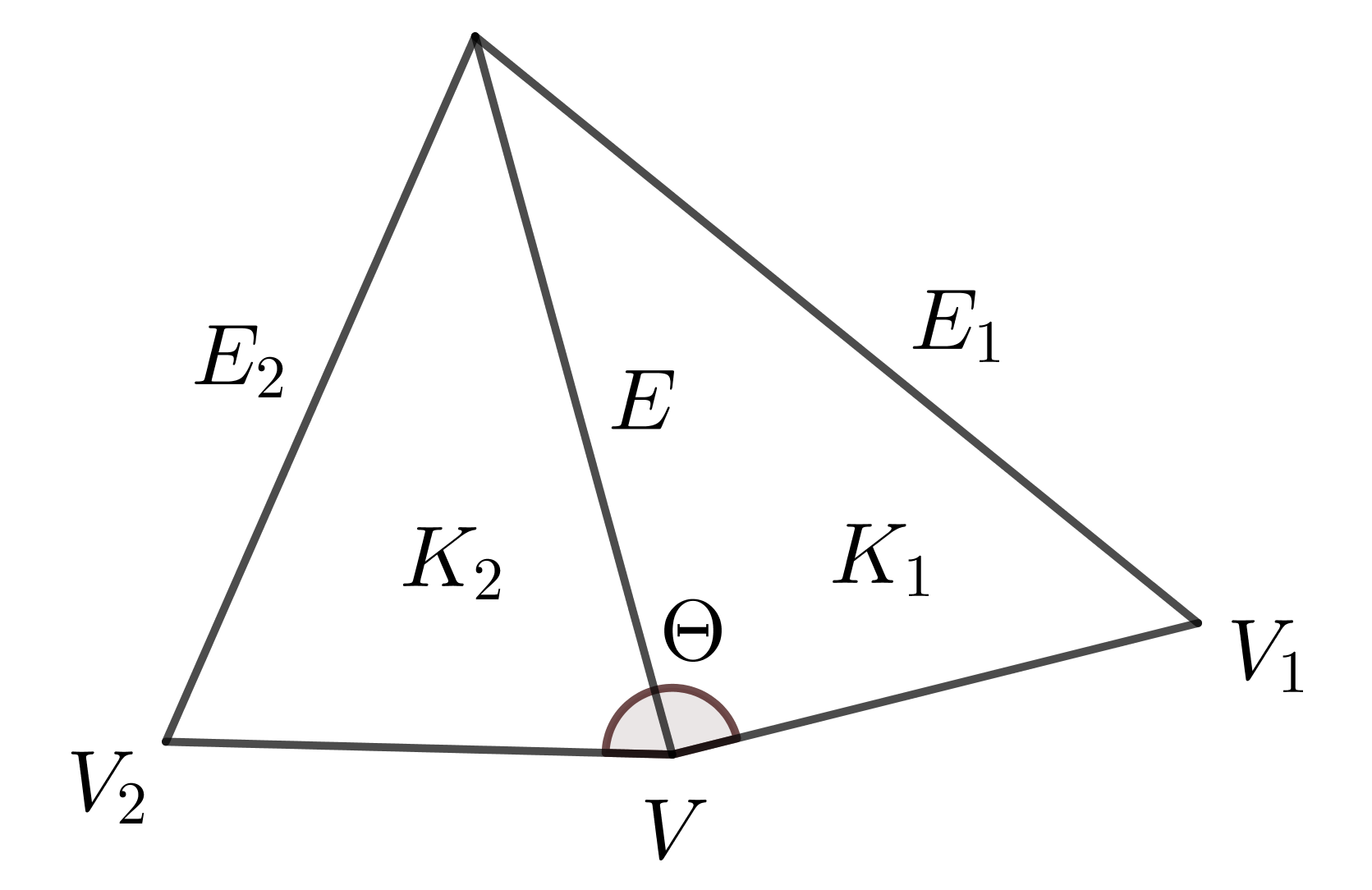
Figure 9: Two back-to-back triangles $K_{1},K_{2}$ sharing a vertex $\mathbf{V}$

We will choose a suitable $\boldsymbol{\xi}$ in (39) to get some inequalities resulted in the following two lemmas. They are useful in estimating the sting error $e_{h}^{\mathbf{V}}$ and postprocessing to remove the spurious error $e_{h}^{\mathbf{V}}$ for quasi singular vertices $\mathbf{V}$.

Lemma 6.4.

Under the same assumption with Lemma 6.3, let $\Theta$ be the angle between $\overrightarrow{\mathbf{V}\mathbf{V}_{1}}$ and $\overrightarrow{\mathbf{V}\mathbf{V}_{2}}$ as in Figure 9. Then,

$$|\alpha_{i}\sin\Theta|\hskip 1.0pt|\overline{\mathbf{V}\mathbf{V}_{i}}|\leq C_{\sigma}(|\mathbf{u}-\mathbf{u}_{h}|_{1,K_{1}\cup K_{2}}+\|p-\Pi_{h}p\|_{0,K_{1}\cup K_{2}}),\quad i=1,2.$$ (46)

Proof.

Choose a unit vector $\boldsymbol{\xi}$ such that

$$\overrightarrow{\mathbf{V}\mathbf{V}_{2}}\cdot\boldsymbol{\xi}=0.$$ (47)

Then

$$|\overrightarrow{\mathbf{V}\mathbf{V}_{1}}\cdot\boldsymbol{\xi}|=|\overline{\mathbf{V}\mathbf{V}_{1}}|\hskip 1.0pt|\cos(\Theta\pm\pi/2)|=|\overline{\mathbf{V}\mathbf{V}_{1}}|\hskip 1.0pt|\sin\Theta|.$$ (48)

From (39), (47), (48), we have (46) for $i=1$. The same argument is repeated for $i=2$. ∎

Lemma 6.5.

Under the same assumption with Lemma 6.3, we have

$$\Big{|}\alpha_{1}|\overline{\mathbf{V}\mathbf{V}_{1}}|+\alpha_{2}|\overline{\mathbf{V}\mathbf{V}_{2}}|\Big{|}\leq C_{\sigma}(|\mathbf{u}-\mathbf{u}_{h}|_{1,K_{1}\cup K_{2}}+\|p-\Pi_{h}p\|_{0,K_{1}\cup K_{2}}).$$

Proof.

Let $\Theta$ be the sum of two angles of $\mathbf{V}$ in $K_{1},K_{2}$ as in Figure 9 and $0\leq{\theta}\leq\pi$ the angle between $\overrightarrow{\mathbf{V}\mathbf{V}_{1}}$ and $-\overrightarrow{\mathbf{V}\mathbf{V}_{2}}$. We note that, if $\Theta\leq\pi$, then $\Theta+{\theta}=\pi$, otherwise, $\Theta-{\theta}=\pi$.

By shape regularity of $\mathcal{T}_{h}$ in (1), (2), $\Theta$ is bounded as

$$2\vartheta_{\sigma}\leq\Theta\leq 2\pi-4\vartheta_{\sigma}.$$ (49)

Thus, in both cases of $\Theta\leq\pi$ or $\Theta>\pi$, we have

$$0\leq{\theta}\leq\pi-2\vartheta_{\sigma}.$$

It means

$$\cos({\theta}/2)=\sqrt{(1+\cos{\theta})/2}\geq\sqrt{(1-\cos 2\vartheta_{\sigma})/2}=\sin\vartheta_{\sigma}>0.$$ (50)

Choose a unit vector $\boldsymbol{\xi}$ so that $\boldsymbol{\xi}$ forms the same acute angle ${\theta}/2$ with $\overrightarrow{\mathbf{V}\mathbf{V}_{1}}$ and $-\overrightarrow{\mathbf{V}\mathbf{V}_{2}}$. Then, from (39), (50), we have

$$\left|\alpha_{1}|\overline{\mathbf{V}\mathbf{V}_{1}}|+\alpha_{2}|\overline{\mathbf{V}\mathbf{V}_{2}}|\right|\leq C_{\sigma}(\sin\vartheta_{\sigma})^{-1}(|\mathbf{u}-\mathbf{u}_{h}|_{1,K_{1}\cup K_{2}}+\|p-\Pi_{h}p\|_{0,K_{1}\cup K_{2}}).$$

∎

6.2 Stable components and spurious error in $e_{h}$

For each vertex $\mathbf{V}$, define the basin $\mathcal{B}(\mathbf{V})$ of $\mathbf{V}$ as the union of all triangles in $\mathcal{T}_{h}$ sharing their common vertex $\mathbf{V}$. For the convenience, we extend the notation as

$$\mathcal{B}(\mathbf{V}_{1},\mathbf{V}_{2},\cdots,\mathbf{V}_{m})=\mathcal{B}(\mathbf{V}_{1})\cup\mathcal{B}(\mathbf{V}_{2})\cup\cdots\cup\mathcal{B}(\mathbf{V}_{m}).$$

The sting error $e_{h}^{\mathbf{V}}$ has a similar property as $e_{h}$ in (31) in the following lemma.

Lemma 6.6.

Let $\mathbf{V}$ be a vertex and $\mathbf{v}_{h}\in X_{h}$. We have

$$(e_{h}^{\mathbf{V}},\mathrm{div}\hskip 1.42262pt\mathbf{v}_{h})\leq C_{\sigma}(|\mathbf{u}-\mathbf{u}_{h}|_{1,\mathcal{B}(\mathbf{V})}+\|p-\Pi_{h}p\|_{0,\mathcal{B}(\mathbf{V})})|\mathbf{v}_{h}|_{1,\mathcal{B}(\mathbf{V})}.$$ (51)

Proof.

(a) interior vertex $\mathbf{V}$

(b) boundary vertex $\mathbf{V}$

Figure 10: Basin $\mathcal{B}(\mathbf{V})$ of a vertex $\mathbf{V}$ (dashed edges belong to $\partial\Omega$.)

Let $K_{1},K_{2},\cdots,K_{m}$ be $m$ triangles in $\mathcal{T}_{h}$ counterclockwisely numbered such that

$$\mathcal{B}(\mathbf{V})=K_{1}\cup K_{2}\cup\cdots\cup K_{m},$$

and $\mathbf{V}_{i}\in K_{i},i=1,2,\cdots,m$ be consecutive vertices on $\partial\mathcal{B}(\mathbf{V})$ as in Figure 10. In case of $\mathbf{V}\in\partial\Omega$, there exists one more vertex $\mathbf{V}_{m+1}\in K_{m}$ on $\partial\mathcal{B}(\mathbf{V})$. If $m=1$, $\mathbf{V}$ belongs to $\partial\Omega$ and as in subsection 4.3,

$$(e_{h}^{\mathbf{V}},\mathrm{div}\hskip 1.42262pt\mathbf{v}_{h})=0.$$

Let $m\geq 2$ and $\ell_{i}=|\overline{\mathbf{V}\mathbf{V}_{i}}|$ and $\boldsymbol{\tau}_{i}=\overrightarrow{\mathbf{V}\mathbf{V}_{i}}/|\overrightarrow{\mathbf{V}\mathbf{V}_{i}}|,\ i=1,2,\cdots,m$. Denoting by $E_{i}$, the opposite edge of $\mathbf{V}$ in $K_{i},i=1,2,\cdots,m$, there exist $m$ constants $\alpha_{1},\alpha_{2},\cdots,\alpha_{m}$ which represent

$$e_{h}^{\mathbf{V}}=\alpha_{1}s_{E_{1}\mathbf{V}}+\alpha_{2}s_{E_{2}\mathbf{V}}+\cdots+\alpha_{m}s_{E_{m}\mathbf{V}}.$$ (52)

Then, from the quadrature rule in Lemma 4.2, we have

$$(e_{h}^{\mathbf{V}},\mathrm{div}\hskip 1.42262pt\mathbf{v}_{h})=\sum_{i=1}^{m}\frac{\ell_{i}}{200}\frac{\partial\mathbf{v}_{h}}{\partial\boldsymbol{\tau}_{i}}(\mathbf{V})\cdot\left(\alpha_{i-1}{\overrightarrow{\mathbf{V}\mathbf{V}_{i-1}}}^{\perp}-\alpha_{i}{\overrightarrow{\mathbf{V}\mathbf{V}_{i+1}}}^{\perp}\right),$$ (53)

where all indexes are modulo $m$, if $\mathbf{V}$ is an interior vertex.

We note that

$$\ell_{i}\Big{|}\frac{\partial\mathbf{v}_{h}}{\partial\boldsymbol{\tau}_{i}}(\mathbf{V})\Big{|}\leq C_{\sigma}|\mathbf{v}_{h}|_{1,K_{i}},\quad i=1,2,\cdots,m.$$ (54)

Thus, the representation in (53) establishes (51) with (54) and Lemma 6.3. ∎

If a vertex $\mathbf{V}$ is not quasi singular, then we estimate $\nabla e_{h}^{\mathbf{V}}$ in the following lemma.

Lemma 6.7.

Let $\mathbf{V}\notin\SS_{h}$ be a regular vertex and $h$ the diameter of the basin $\mathcal{B}(\mathbf{V})$. Then we have

$$h\|\nabla e_{h}^{\mathbf{V}}\|_{0,\mathcal{B}(\mathbf{V})}=C_{\sigma}(|\mathbf{u}-\mathbf{u}_{h}|_{1,\mathcal{B}(\mathbf{V})}+\|p-\Pi_{h}p\|_{0,\mathcal{B}(\mathbf{V})}).$$ (55)

Proof.

Under the same notations in the proof of Lemma 6.6, from the definition of $\SS_{h}$ in (3), there exist two back-to-back triangles $K_{j},K_{j+1}$ such that the sum $\Theta$ of their angles of $\mathbf{V}$ satisfies

$$|\Theta-\pi|\geq\vartheta_{\sigma}.$$ (56)

Then, from (49), (56), we have $|\sin\vartheta_{\sigma}|\leq|\sin\Theta|$. Thus, by Lemma 6.4, $|\alpha_{j}|$ in (52) is bounded by

$$h^{-1}C_{\sigma}(|\mathbf{u}-\mathbf{u}_{h}|_{1,\mathcal{B}(\mathbf{V})}+\|p-\Pi_{h}p\|_{0,\mathcal{B}(\mathbf{V})}),$$

and sequentially so are all $|\alpha_{i}|,i=1,2,\cdots,m$ in (52) by Lemma 6.5. It implies (55), since

$$\|\nabla s_{E_{i}\mathbf{V}}\|_{0,K_{i}}\leq C_{\sigma},\quad i=1,2,\cdots,m.$$

∎

Split the sting error $e_{h}^{S}$ into two components by regular and quasi singular vertices:

$$e_{h}^{S}=e_{h}^{SR}+e_{h}^{SS},$$ (57)

where

$$e_{h}^{SR}=\sum_{\mathbf{V}\notin\SS_{h}}e_{h}^{\mathbf{V}},\quad e_{h}^{SS}=\sum_{\mathbf{V}\in\SS_{h}}e_{h}^{\mathbf{V}}.$$

Then the components $e_{h}^{G},e_{h}^{SR}$ in $e_{h}=e_{h}^{G}+e_{h}^{SR}+e_{h}^{SS}$ is stable as in the following theorem.

Theorem 6.8.

Let $\mathpzc{m}$ be the mean of $e_{h}^{G}+e_{h}^{SR}$ over $\Omega$. Then, if $\mathbf{u}\in[H^{5}(\Omega)]^{2},p\in H^{4}(\Omega)$, we have

$$\|e_{h}^{G}+e_{h}^{SR}-\mathpzc{m}\|_{0}\leq Ch^{4}(|\mathbf{u}|_{5}+|p|_{4}).$$ (58)

Proof.

Denote $e_{h}^{G}+e_{h}^{SR}-\mathpzc{m}$ by $e_{h}^{GR\mathpzc{m}}$. Let $\Pi_{h}e_{h}^{GR\mathpzc{m}}$ be the projection of $e_{h}^{GR\mathpzc{m}}\in L_{0}^{2}(\Omega)$ into $\mathcal{P}_{0,h}(\Omega)$. Then, from the stability of $P^{2}-P^{0}$ [1], there exists $\mathbf{v}_{h}\in X_{h}$ such that

$$(\Pi_{h}e_{h}^{GR\mathpzc{m}},e_{h}^{GR\mathpzc{m}}-\mathrm{div}\hskip 1.42262pt\mathbf{v}_{h})=0,\quad|\mathbf{v}_{h}|_{1}\leq C\|e_{h}^{GR\mathpzc{m}}\|_{0}.$$ (59)

We note, by Theorem 3.2 and Lemma 6.1, 6.7,

$$\|e_{h}^{GR\mathpzc{m}}-\Pi_{h}e_{h}^{GR\mathpzc{m}}\|_{0}\leq Ch^{4}(|\mathbf{u}|_{5}+|p|_{4}).$$ (60)

Then, Lemma 6.6 helps us to estimate (58) with (31), (59), (60) in the following expansion:

$$\begin{array}[]{ccl}\|e_{h}^{GR\mathpzc{m}}\|_{0}^{2}&=&(e_{h}^{GR\mathpzc{m}},e_{h}^{GR\mathpzc{m}}-\mathrm{div}\hskip 1.42262pt\mathbf{v}_{h})+(e_{h}^{GR\mathpzc{m}},\mathrm{div}\hskip 1.42262pt\mathbf{v}_{h})\\ &=&(e_{h}^{GR\mathpzc{m}}-\Pi_{h}e_{h}^{GR\mathpzc{m}},e_{h}^{GR\mathpzc{m}}-\mathrm{div}\hskip 1.42262pt\mathbf{v}_{h})+(e_{h}^{GR\mathpzc{m}},\mathrm{div}\hskip 1.42262pt\mathbf{v}_{h})\\ &\leq&Ch^{4}(|\mathbf{u}|_{5}+|p|_{4})\|e_{h}^{GR\mathpzc{m}}\|_{0}+(e_{h}^{GR\mathpzc{m}},\mathrm{div}\hskip 1.42262pt\mathbf{v}_{h})\\ &=&Ch^{4}(|\mathbf{u}|_{5}+|p|_{4})\|e_{h}^{GR\mathpzc{m}}\|_{0}+(e_{h},\mathrm{div}\hskip 1.42262pt\mathbf{v}_{h})-(e_{h}^{SS},\mathrm{div}\hskip 1.42262pt\mathbf{v}_{h})\\ &\leq&Ch^{4}(|\mathbf{u}|_{5}+|p|_{4})(\|e_{h}^{GR\mathpzc{m}}\|_{0}+|\mathbf{v}_{h}|_{1})\leq Ch^{4}(|\mathbf{u}|_{5}+|p|_{4})\|e_{h}^{GR\mathpzc{m}}\|_{0}.\end{array}$$

∎

If $\mathcal{T}_{h}$ has no quasi singular vertex, Theorem 6.8 asserts that $p_{h}-p$ has an error decay of optimal order as expected from the inf-sup condition in (8).

The presence of quasi singular vertices, however, the sting error $e_{h}^{SS}$ could appear as large as spoiling the discrete pressure $p_{h}$ as in Figure 15 in the last section. In the next section, we are going to postprocess $p_{h}$ to remove $e_{h}^{SS}$ which is called spurious error.

7 Remove spurious error $e_{h}^{SS}$

We will postprocess $p_{h}$ to remove the undesired error $e_{h}^{\mathbf{V}}$ in the following order:

1. $e_{h}^{\mathbf{V}}$ for interior quasi singular vertices $\mathbf{V}$ using the jump of $p_{h}$ at $\mathbf{V}$,

2. $e_{h}^{\mathbf{V}}$ for boundary quasi singular vertices $\mathbf{V}$ away from corners using the jump at $\mathbf{V}$,

3. $e_{h}^{\mathbf{V}}$ for boundary quasi singular corners $\mathbf{V}$ using the jump at the opposite edge.

Dividing quasi singular vertices by interior and boundary into

$$\SS_{h}^{i}=\{\mathbf{V}\in\SS_{h}\ |\ \mathbf{V}\notin\partial\Omega\},\quad\SS_{h}^{b}=\{\mathbf{V}\in\SS_{h}\ |\ \mathbf{V}\in\partial\Omega\},$$

we split the spurious error $e_{h}^{SS}$ into

$$e_{h}^{SS}=e_{h}^{SSi}+e_{h}^{SSb},$$ (61)

where

$$e_{h}^{SSi}=\sum_{\mathbf{V}\in\SS_{h}^{i}}e_{h}^{\mathbf{V}},\quad e_{h}^{SSb}=\sum_{\mathbf{V}\in\SS_{h}^{b}}e_{h}^{\mathbf{V}}.$$

7.1 Remove interior spurious error $e_{h}^{SSi}$

Let $\mathbf{V}\in\SS_{h}^{i}$ be an interior quasi singular vertex, then the basin $\mathcal{B}(\mathbf{V})$ of $\mathbf{V}$ consists of 4 triangles $K_{1},K_{2},K_{3},K_{4}$ by Lemma 2.1. In this subsection, we adopt the notations in Figure 10-(a). Note that 4 unknown constants $\alpha_{1},\alpha_{2},\alpha_{3},\alpha_{4}$ represent $e_{h}^{\mathbf{V}}$ as

$$e_{h}^{\mathbf{V}}=\alpha_{1}s_{E_{1}\mathbf{V}}+\alpha_{2}s_{E_{2}\mathbf{V}}+\alpha_{3}s_{E_{3}\mathbf{V}}+\alpha_{4}s_{E_{4}\mathbf{V}}.$$ (62)

By Lemma 6.5, $\alpha_{1},\alpha_{2}$ satisfy

$$|\alpha_{1}\ell_{1}+\alpha_{2}\ell_{3}|\leq C_{\sigma}(|\mathbf{u}-\mathbf{u}_{h}|_{1,K_{1}\cup K_{2}}+\|p-\Pi_{h}p\|_{0,K_{1}\cup K_{2}}).$$ (63)

Note that $e_{h}^{SS}\big{|}_{\mathcal{B}(\mathbf{V})}=e_{h}^{\mathbf{V}}$, since $\mathbf{V}$ is the only quasi singular vertex in $\mathcal{B}(\mathbf{V})$ by Lemma 2.2. Thus, from (33), (57), (62), we have

$$e_{h}\Big{|}_{K_{1}}=(e_{h}^{G}+e_{h}^{SR})\Big{|}_{K_{1}}+\alpha_{1}s_{E_{1}\mathbf{V}},\quad e_{h}\Big{|}_{K_{2}}=(e_{h}^{G}+e_{h}^{SR})\Big{|}_{K_{2}}+\alpha_{2}s_{E_{2}\mathbf{V}}.$$ (64)

Define a jump of a function $f$ at $\mathbf{V}$ as

$$[[f]]_{\mathbf{V}}=f|_{K_{1}}(\mathbf{V})-f|_{K_{2}}(\mathbf{V}).$$

Then, since $\Pi_{h}p$ has no jump at $\mathbf{V}$ and $s_{E_{1}\mathbf{V}}(\mathbf{V})=s_{E_{2}\mathbf{V}}(\mathbf{V})=1$, (64) makes

$$[[p_{h}]]_{\mathbf{V}}=[[e_{h}]]_{\mathbf{V}}=[[e_{h}^{G}+e_{h}^{SR}]]_{\mathbf{V}}+\alpha_{1}-\alpha_{2}.$$ (65)

Roughly speaking, (63) and (65) help us to get $\alpha_{1},\alpha_{2}$ with $[[p_{h}]]_{\mathbf{V}}$ which we can calculate.

Choose two constants $\gamma_{1},\gamma_{2}$ so that

$$\gamma_{1}\ell_{1}+\gamma_{2}\ell_{3}=0,\quad\gamma_{1}-\gamma_{2}=[[p_{h}]]_{\mathbf{V}}.$$ (66)

Then, the differences $\alpha_{1}-\gamma_{1},\alpha_{2}-\gamma_{2}$ are estimated in the following lemma.

Lemma 7.1.

Let $\mathpzc{m}$ be the mean of $e_{h}^{G}+e_{h}^{SR}$ over $\Omega$. Then we have, for $i=1,2$,

$$\|(\alpha_{i}-\gamma_{i})s_{E_{i}\mathbf{V}}\|_{0,K_{i}}\leq C_{\sigma}(\|e_{h}^{G}+e_{h}^{SR}-\mathpzc{m}\|_{0,K_{1}\cup K_{2}}+|\mathbf{u}-\mathbf{u}_{h}|_{1,K_{1}\cup K_{2}}+\|p-\Pi_{h}p\|_{0,K_{1}\cup K_{2}}).$$ (67)

Proof.

By (63), (65), (66), the differences $d_{1}=\alpha_{1}-\gamma_{1},d_{2}=\alpha_{2}-\gamma_{2}$ satisfy

$$|d_{1}\ell_{1}+d_{2}\ell_{3}|\leq C_{\sigma}(|\mathbf{u}-\mathbf{u}_{h}|_{1,K_{1}\cup K_{2}}+\|p-\Pi_{h}p\|_{0,K_{1}\cup K_{2}}),\quad d_{1}-d_{2}+[[e_{h}^{G}+e_{h}^{SR}]]_{\mathbf{V}}=0.$$ (68)

The equation in (68) induces that

$$|d_{1}-d_{2}|\leq C_{\sigma}(\ell_{1}^{-1}\|e_{h}^{G}+e_{h}^{SR}-\mathpzc{m}\|_{K_{1}}+\ell_{3}^{-1}\|e_{h}^{G}+e_{h}^{SR}-\mathpzc{m}\|_{K_{2}}),$$ (69)

since

$$[[e_{h}^{G}+e_{h}^{SR}]]_{\mathbf{V}}=(e_{h}^{G}+e_{h}^{SR}-\mathpzc{m})\Big{|}_{K_{1}}(\mathbf{V})-(e_{h}^{G}+e_{h}^{SR}-\mathpzc{m})\Big{|}_{K_{2}}(\mathbf{V}).$$

Note that

$$\|s_{E_{1}\mathbf{V}}\|_{0,K_{1}}\leq C_{\sigma}\ell_{1},\quad\|s_{E_{2}\mathbf{V}}\|_{0,K_{2}}\leq C_{\sigma}\ell_{3}.$$ (70)

Then, combining (68)-(70), the estimation (67) comes from the following identities:

$$(\ell_{1}+\ell_{3})d_{1}=(d_{1}\ell_{1}+d_{2}\ell_{3})+\ell_{3}(d_{1}-d_{2}),\quad(\ell_{1}+\ell_{3})d_{2}=(d_{1}\ell_{1}+d_{2}\ell_{3})-\ell_{1}(d_{1}-d_{2}).$$

∎

For another pair of two triangles $K_{3},K_{4}$, we can choose $\gamma_{3},\gamma_{4}$ in the similar way of $\gamma_{1},\gamma_{2}$.

Now, for each interior quasi singular vertex $\mathbf{V}\in\SS_{h}^{i}$, calculate such $\gamma_{1},\gamma_{2},\gamma_{3},\gamma_{4}$ and define

$$s_{h}^{\mathbf{V}}=\gamma_{1}s_{E_{1}\mathbf{V}}+\gamma_{2}s_{E_{2}\mathbf{V}}+\gamma_{3}s_{E_{3}\mathbf{V}}+\gamma_{4}s_{E_{4}\mathbf{V}},$$

and

$$s_{h}^{i}=\sum_{\mathbf{V}\in\SS_{h}^{i}}s_{h}^{\mathbf{V}}.$$ (71)

Then, from Theorem 3.2, 6.8 and Lemma 7.1, we establish the following lemma.

Lemma 7.2.

If $\mathbf{u}\in[H^{5}(\Omega)]^{2},p\in H^{4}(\Omega)$, we have

$$\|e_{h}^{SSi}-s_{h}^{i}\|_{0}\leq Ch^{4}(|\mathbf{u}|_{5}+|p|_{4}).$$ (72)

7.2 Remove boundary spurious error $e_{h}^{SSb}$

We have known $p_{h}$ and $s_{h}^{i}$ such that

$$p_{h}-s_{h}^{i}-\Pi_{h}p=e_{h}^{G}+e_{h}^{SR}+e_{h}^{SSi}-s_{h}^{i}+e_{h}^{SSb}.$$ (73)

In this subsection, we will deal with the error $e_{h}^{SSb}$ in (73) for boundary quasi singular vertices.

Denote by $\mathcal{R}_{h}$, the set all regular vertices, that is $\mathcal{R}_{h}=\mathcal{V}_{h}\setminus\SS_{h}$. Let $\partial\Omega\setminus\mathcal{R}_{h}$ consist of $J$ components $\mathpzc{s}_{1},\mathpzc{s}_{2},_{3},\cdots,\mathpzc{s}_{J}$ and define quasi singular chains as

$$\mathpzc{Q}_{j}=\mathcal{V}_{h}\cap\mathpzc{s}_{j},\quad j=1,2,\cdots,J.$$

Note $\mathpzc{Q}_{1},\mathpzc{Q}_{2},\cdots,\mathpzc{Q}_{J}$ are sets of consecutive boundary quasi singular vertices separated by regular vertices. We will first remove spurious error for all quasi singular chains which do not contain any corner of $\partial\Omega$ in subsubsection 7.2.1 below. Then we will go to the remaining quasi singular chains having a corner in subsubsection 7.2.2.

Let $\SS_{h}^{br}$ be the union of all quasi singular chains not having any corner and $\SS_{h}^{bc}=\SS_{h}^{b}\setminus\SS_{h}^{br}$. Then, split $e_{h}^{SSb}$ into

$$e_{h}^{SSb}=e_{h}^{SSbr}+e_{h}^{SSbc},$$ (74)

where

$$e_{h}^{SSbr}=\sum_{\mathbf{V}\in\SS_{h}^{br}}e_{h}^{\mathbf{V}},\quad e_{h}^{SSbc}=\sum_{\mathbf{V}\in\SS_{h}^{bc}}e_{h}^{\mathbf{V}}.$$

In the remaining analysis, we will use the notations in this paragraph. Let $\mathpzc{S}$ be a set of $m+2$ consecutive vertices on a line segment of $\partial\Omega$ such that

$$\mathpzc{S}=\{\mathbf{V}_{0},\mathbf{V}_{1},\cdots,\mathbf{V}_{m},\mathbf{V}_{m+1}\},$$ (75)

as in Figure 11. Assume $\mathbf{V}_{1},\mathbf{V}_{2},\cdots,\mathbf{V}_{m}$ are quasi singular, actually exact singular. Then, there exists a vertex $\mathbf{W}$ such that, for each $k\in\{0,1,2,\cdots,m+1\}$, there is an edge $E_{k}$ which connects $\mathbf{W}$ and $\mathbf{V}_{k}$. Let $K_{k}$ be the triangle with vertices $\mathbf{V}_{k-1},\mathbf{V}_{k},\mathbf{W}$ and $\ell_{k}=|\mathbf{V}_{k-1}\mathbf{V}_{k}|,\ k=1,2,\cdots,m+1.$

Figure 11: Consecutive boundary singular vertices $\mathbf{V}_{1},\mathbf{V}_{2},\mathbf{V}_{3}$

To avoid pathological meshes as the examples in Figure 12, we assume the following on the triangulation $\mathcal{T}_{h}$:

Assumption 7.1.

1. Each line segment of $\partial\Omega$ connecting two corner of $\partial\Omega$ has at least two regular vertices.

2. Each quasi singular vertex which is a corner of $\partial\Omega$ has no interior edge connecting it to other boundary vertex.

(a) Each boundary segment has only one regular vertex.

(b) A quasi singular corner $\mathbf{V}$ is connected to other boundary vertex by an interior edge.

Figure 12: Examples of pathological meshes (dashed lines belong to $\partial\Omega$.)

7.2.1 Quasi singular chain not having any corner

Let $\mathpzc{Q}$ be a quasi singular chain which does not have any corner. We can set in (75) that

$$\mathpzc{Q}=\{\mathbf{V}_{1},\mathbf{V}_{2},\cdots,\mathbf{V}_{m}\}\quad\mbox{ for }m\geq 1,$$

and $\mathbf{V}_{0},\mathbf{V}_{m+1}$ are regular vertices.

Then, we note that $\mathbf{W}$ is also regular. It is clear by Lemma 2.2 if $\mathbf{W}$ is an interior vertex. In case of $\mathbf{W}\in\partial\Omega$, $\mathbf{W}$ is not a corner as in Figure 12-(b) by Assumption 7.1. Thus, $\mathbf{W}$ is regular on a line segment of $\partial\Omega$ since $m\geq 1$.

We can represent $e_{h}^{\mathbf{V}_{k}}$ with unknown constants $\alpha_{k},\beta_{k}$ as

$$e_{h}^{\mathbf{V}_{k}}=\alpha_{k}s_{E_{k-1}\mathbf{V}_{k}}+\beta_{k}s_{E_{k+1}\mathbf{V}_{k}}\quad k=1,2,\cdots,m.$$ (76)

Then, by Lemma 6.5, we have, for $k=1,2,\cdots,m$,

$$|\alpha_{k}\ell_{k}+\beta_{k}\ell_{k+1}|\leq C_{\sigma}(|\mathbf{u}-\mathbf{u}_{h}|_{1,\mathcal{B}(\mathbf{V}_{k})}+\|p-\Pi_{h}p\|_{0,\mathcal{B}(\mathbf{V}_{k})}).$$ (77)

We note that $\mathbf{V}_{1},\mathbf{V}_{2},\cdots,\mathbf{V}_{m}$ are the only quasi singular vertices in $\mathcal{B}(\mathbf{V}_{1},\mathbf{V}_{2},\cdots,\mathbf{V}_{m})$ since $\mathbf{V}_{0},\mathbf{V}_{m+1},\mathbf{W}$ are regular. Thus, from (33), (57), (76), we have

$$\begin{array}[]{c}e_{h}\Big{|}_{K_{1}}=(e_{h}^{G}+e_{h}^{SR})\Big{|}_{K_{1}}+\alpha_{1}s_{E_{0}\mathbf{V}_{1}},\quad e_{h}\Big{|}_{K_{m+1}}=(e_{h}^{G}+e_{h}^{SR})\Big{|}_{K_{m+1}}+\beta_{m}s_{E_{m+1}\mathbf{V}_{m}},\\ e_{h}\Big{|}_{K_{k}}=(e_{h}^{G}+e_{h}^{SR})\Big{|}_{K_{k}}+\alpha_{k}s_{E_{k-1}\mathbf{V}_{k}}+\beta_{k-1}s_{E_{k}\mathbf{V}_{k-1}},\quad k=2,3,\cdots,m.\end{array}$$ (78)

Define a jump of a function $f$ at $\mathbf{V}_{k}$ as

$$[[f]]_{\mathbf{V}_{k}}=f|_{K_{k}}(\mathbf{V}_{k})-f|_{K_{k+1}}(\mathbf{V}_{k}),\quad k=1,2,\cdots,m.$$

Then, from (78), we have, for $k=1,2,\cdots,m$,

$$[[p_{h}]]_{\mathbf{V}_{k}}=[[e_{h}]]_{\mathbf{V}_{k}}=(\alpha_{k}-\frac{1}{10}\beta_{k-1})-(\beta_{k}-\frac{1}{10}\alpha_{k+1})+[[e_{h}^{G}+e_{h}^{SR}]]_{\mathbf{V}_{k}},$$ (79)

with the definition of sting functions in (12). In (79), $\beta_{0}=\alpha_{m+1}=0$.

We can find $2m$ scalars $\widetilde{\alpha}_{1},\widetilde{\beta}_{1},\widetilde{\alpha}_{2},\widetilde{\beta}_{2},\cdots,\widetilde{\alpha}_{m},\widetilde{\beta}_{m}$ such that

$$\widetilde{\alpha}_{k}\ell_{k}+\widetilde{\beta}_{k}\ell_{k+1}=0,\quad[[p_{h}]]_{\mathbf{V}_{k}}=(\widetilde{\alpha}_{k}-\frac{1}{10}\widetilde{\beta}_{k-1})-(\widetilde{\beta}_{k}-\frac{1}{10}\widetilde{\alpha}_{k+1}),\quad k=1,2,\cdots,m,$$ (80)

where $\widetilde{\beta}_{0}=\widetilde{\alpha}_{m+1}=0$. Note that the conditions in (80) are similar to those in (77), (79). The existence of $\widetilde{\alpha}_{k},\widetilde{\beta}_{k}$ is guaranteed by the argument in the proof of Lemma 7.3 below.

Define discrete pressures $s_{h}^{\mathbf{V}_{k}}$ as

$$s_{h}^{\mathbf{V}_{k}}=\widetilde{\alpha}_{k}s_{E_{k-1}\mathbf{V}_{k}}+\widetilde{\beta}_{k}s_{E_{k+1}\mathbf{V}_{k}},\quad k=1,2,\cdots,m.$$ (81)

Then, the difference $e_{h}^{\mathbf{V}_{k}}-s_{h}^{\mathbf{V}_{k}}$ is estimated in the following lemma.

Lemma 7.3.

Let $\mathpzc{m}$ be the mean of $e_{h}^{G}+e_{h}^{SR}$ over $\Omega$ Then, we have, for $k=1,2,\cdots,m$,

$$\|e_{h}^{\mathbf{V}_{k}}-s_{h}^{\mathbf{V}_{k}}\|_{0,\mathcal{B}(\mathbf{V}_{k})}\leq C_{\sigma}(\|e_{h}^{G}+e_{h}^{SR}-\mathpzc{m}\|_{0,\mathcal{B}(\mathbf{W})}+|\mathbf{u}-\mathbf{u}_{h}|_{1,\mathcal{B}(\mathbf{W})}+\|p-\Pi_{h}p\|_{0,\mathcal{B}(W)}).$$ (82)

Proof.

Let $\hat{\alpha}_{k}=\alpha_{k}-\widetilde{\alpha}_{k},\ \hat{\beta}_{k}=\beta_{k}-\widetilde{\beta}_{k},\ k=1,2,\cdots,m$ and $\hat{\beta}_{0}=\hat{\alpha}_{m+1}=0$. Then from (77)-(80), we have

$$\begin{array}[]{c}|\hat{\alpha}_{k}\ell_{k}+\hat{\beta}_{k}\ell_{k+1}|\leq C_{\sigma}(|\mathbf{u}-\mathbf{u}_{h}|_{1,\mathcal{B}(\mathbf{V}_{k})}+\|p-\Pi_{h}p\|_{0,\mathcal{B}(\mathbf{V}_{k})}),\\ (\hat{\alpha}_{k}-\displaystyle\frac{1}{10}\hat{\beta}_{k-1})-(\hat{\beta}_{k}-\displaystyle\frac{1}{10}\hat{\alpha}_{k+1})+[[e_{h}^{S}+e_{h}^{SR}]]_{\mathbf{V}_{k}}=0.\end{array}$$ (83)

Set $a_{m+1}=0$ and for $k=1,2,\cdots,m$,

$$r_{k}=\frac{\ell_{k+1}}{\ell_{k}},\ a_{k}=\hat{\alpha}_{k}+r_{k}\hat{\beta}_{k},\ b_{k}=a_{k}+\frac{1}{10}a_{k+1}-(\hat{\alpha}_{k}-\frac{1}{10}\hat{\beta}_{k-1})+(\hat{\beta}_{k}-\frac{1}{10}\hat{\alpha}_{k+1}).$$ (84)

Then, eliminating $\hat{\alpha}_{1},\hat{\alpha}_{2},\cdots,\hat{\alpha}_{m+1}$ in (84), we have $m$ equations for $\hat{\beta}_{1},\hat{\beta}_{2},\cdots,\hat{\beta}_{m}$,

$$\frac{1}{10}\hat{\beta}_{k-1}+(1+r_{k})\hat{\beta}_{k}+\frac{1}{10}r_{k+1}\hat{\beta}_{k+1}=b_{k},\quad k=1,2,\cdots,m,$$ (85)

where $\hat{\beta}_{0}=\hat{\beta}_{m+1}=r_{m+1}=0$.

Rewrite (85) with a matrix $A\in\mathbb{R}^{m\times m}$ in the form:

$$A(\hat{\beta}_{1},\hat{\beta}_{2},\cdots,\hat{\beta}_{m})^{t}=(b_{1},b_{2},\cdots,b_{m}).^{t}$$ (86)

For an example when $m=4$, since $\hat{\beta}_{0}=\hat{\beta}_{5}=0$, (85) is written in

$$\left(\begin{array}[]{cccc}1+r_{1}&r_{2}/{10}&&\\ 1/{10}&1+r_{2}&r_{3}/{10}&\\ &1/{10}&1+r_{3}&r_{4}/{10}\\ &&1/{10}&1+r_{4}\\ \end{array}\right)\left(\begin{array}[]{c}\hat{\beta}_{1}\\ \hat{\beta}_{2}\\ \hat{\beta}_{3}\\ \hat{\beta}_{4}\end{array}\right)=\left(\begin{array}[]{c}b_{1}\\ b_{2}\\ b_{3}\\ b_{4}\end{array}\right).$$ (87)

Note that $A$ is invertible since the transpose $A^{t}$ is strictly diagonally dominant. Thus, we have

$${\left|\kern-1.07639pt\left|\kern-1.07639pt\left|A^{-1}\right|\kern-1.07639pt\right|\kern-1.07639pt\right|}_{2}\leq C_{\sigma},$$ (88)

since $m$ and $r_{1},r_{2},\cdots,r_{m}$ are bounded by $C_{\sigma}$. From (76), (81), (83), (84), (86), (88), we obtain (82) with $a_{k}=(\hat{\alpha}_{k}\ell_{k}+\hat{\beta}_{k}\ell_{k+1})/\ell_{k},\ k=1,2,\cdots,m.$ ∎

Now, for each $\mathbf{V}\in\SS_{h}^{br}$, we can calculate $s_{h}^{\mathbf{V}}$ similarly in (80), (81) and define

$$s_{h}^{br}=\sum_{\mathbf{V}\in\SS_{h}^{br}}s_{h}^{\mathbf{V}}.$$ (89)

Then, from Theorem 3.2, 6.8 and Lemma 7.3, we establish the following lemma.

Lemma 7.4.

If $\mathbf{u}\in[H^{5}(\Omega)]^{2},p\in H^{4}(\Omega)$, we have

$$\|e_{h}^{SSbr}-s_{h}^{br}\|_{0}\leq Ch^{4}(|\mathbf{u}|_{5}+|p|_{4}).$$ (90)

7.2.2 Quasi singular chain having a corner

Let $\widehat{p}_{h}=p_{h}-s_{h}^{i}-s_{h}^{br}$ and define

$$\widehat{e}_{h}=\widehat{p}_{h}-\Pi_{h}p=e_{h}^{G}+e_{h}^{SR}+e_{h}^{SSi}-s_{h}^{i}+e_{h}^{SSbr}-s_{h}^{br}+e_{h}^{SSbc}.$$ (91)

The remaining spurious error $e_{h}^{SSbc}$ in (91) is our last target to be removed.

Let $\mathpzc{Q}$ be a quasi singular chain containing a corner $\mathbf{C}$ of two line segments $\Gamma,\Gamma_{1}$ of $\partial\Omega$ such that

$$\#(\mathpzc{Q}\cap\Gamma_{1})\ \leq\ \#(\mathpzc{Q}\cap\Gamma).$$ (92)

We can set in (75) that

$$\mathpzc{Q}\cap\Gamma=\{\mathbf{V}_{0},\mathbf{V}_{1},\mathbf{V}_{2},\cdots,\mathbf{V}_{m}\}\quad\mbox{ for }m\geq 0,$$

and $\mathbf{V}_{0}$ is the quasi singular corner $\mathbf{C}$ and $\mathbf{V}_{m+1}$ is a regular vertex $\mathbf{R}$.

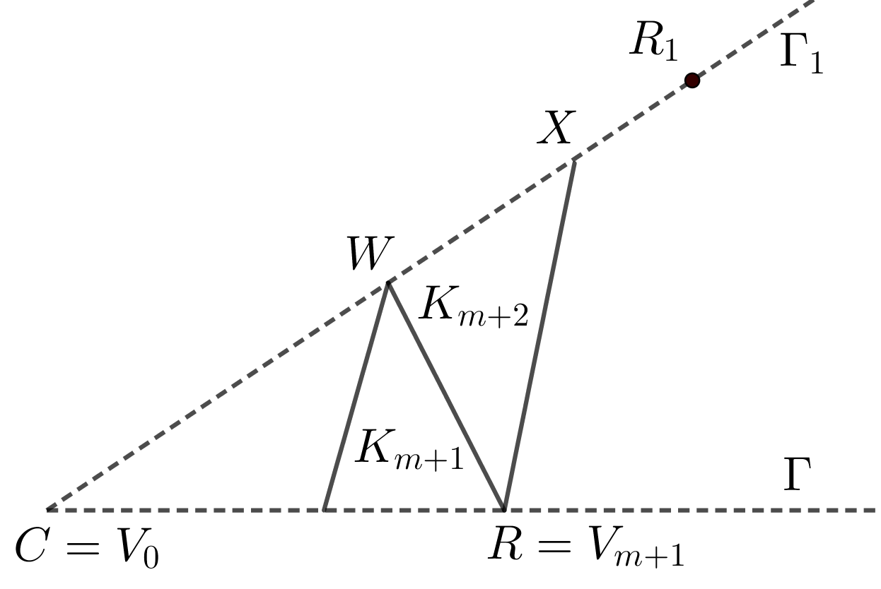
(a) $\mathbf{W}\in\partial\Omega$

(b) $\mathbf{W}\notin\partial\Omega$

Figure 13: $\mathbf{W},\mathbf{X}\notin\SS_{h}^{bc}$ and the postprocessing starts at $K_{m+2}$. (dashed lines belong to $\partial\Omega$.)

Then, by Assumption 7.1, $\mathbf{V}_{m+1}$ is not a corner. Thus, there exists a triangle $K_{m+2}$ in $\mathcal{T}_{h}$ which has the edge $E_{m+1}$ and a vertex $X$ different to $\mathbf{V}_{m}$ as in Figure 13.

We remind that $\SS_{h}^{bc}$ is the set of all boundary quasi singular vertices consecutive from quasi singular corners. If $\mathbf{W}\in\SS_{h}^{bc}$, then $\mathbf{W}$ is quasi singular in $\mathpzc{Q}\cap\Gamma_{1}$ and $m=0$. It contradicts to (92). Thus $\mathbf{W}\notin\SS_{h}^{bc}$.

For the vertex $\mathbf{X}$, if $\mathbf{X}\in\SS_{h}^{bc}$, then $\mathbf{W},\mathbf{X}$ lie on $\Gamma_{1}$ as in Figure 13-(a), since $\mathbf{X}$ must be on a boundary line segment and $\mathbf{W},\mathbf{R}$ can not be corners by Assumption 7.1. While $\mathbf{W}\notin\SS_{h}^{bc}$ is regular, there exists one more regular vertex on $\Gamma_{1}$ by Assumption 7.1, presented as $\mathbf{R}_{1}$ in Figure 13-(a). It conflicts with $\mathbf{X}\in\SS_{h}^{bc}$. Thus, we have $\mathbf{X}\notin\SS_{h}^{bc}$, too.

With $2m+1$ unknown constants $\beta_{0},\alpha_{1},\beta_{1},\alpha_{2},\beta_{2},\cdots,\alpha_{m},\beta_{m}$, we can represent that

$$e_{h}^{\mathbf{C}}\Big{|}_{K_{1}}=\beta_{0}s_{E_{1}\mathbf{C}},\quad e_{h}^{\mathbf{V}_{k}}=\alpha_{k}s_{E_{k-1}\mathbf{V}_{k}}+\beta_{k}s_{E_{k+1}\mathbf{V}_{k}}\quad k=1,2,\cdots,m.$$ (93)

We note that $e_{h}^{SSbc}\big{|}_{K_{m+2}}=0$ since $\mathbf{R},\mathbf{W},\mathbf{X}\notin\SS_{h}^{bc}$. Thus, from (91), (93), we have

$$\begin{array}[]{lcl}\widehat{e}_{h}|_{K_{m+2}}&=&(e_{h}^{G}+e_{h}^{SR}+e_{h}^{SSi}-s_{h}^{i}+e_{h}^{SSbr}-s_{h}^{br})\Big{|}_{K_{m+2}},\\ \widehat{e}_{h}|_{K_{m+1}}&=&(e_{h}^{G}+e_{h}^{SR}+e_{h}^{SSi}-s_{h}^{i}+e_{h}^{SSbr}-s_{h}^{br})\Big{|}_{K_{m+1}}+\beta_{m}s_{E_{m+1}\mathbf{V}_{m}},\end{array}$$ (94)

and for $k=1,2,\cdots,m$,

$$\widehat{e}_{h}\Big{|}_{K_{k}}=(e_{h}^{G}+e_{h}^{SR}+e_{h}^{SSi}-s_{h}^{i}+e_{h}^{SSbr}-s_{h}^{br})\Big{|}_{K_{k}}+\alpha_{k}s_{E_{k-1}\mathbf{V}_{k}}+\beta_{k-1}s_{E_{k}\mathbf{V}_{k-1}}.$$

Denote by $\mathbf{M}$, the midpoint of the edge $\overline{\mathbf{R}\mathbf{W}}$ and define a jump of a function $f$ at $\mathbf{M}$ as

$$[[f]]_{\mathbf{M}}=f\big{|}_{K_{m+1}}(\mathbf{M})-f\big{|}_{K_{m+2}}(\mathbf{M}).$$

Then, from (94), we have

$$[[\widehat{p}_{h}]]_{\mathbf{M}}=[[\widehat{e}_{h}]]_{\mathbf{M}}=-\frac{1}{10}\beta_{m}+[[e_{h}^{G}+e_{h}^{SR}+e_{h}^{SSi}-s_{h}^{i}+e_{h}^{SSbr}-s_{h}^{br}]]_{\mathbf{M}},$$ (95)

and for $k=1,2,\cdots,m$ and $\alpha_{m+1}=0$, we have

$$[[\widehat{p}_{h}]]_{\mathbf{V}_{k}}=(\alpha_{k}-\frac{1}{10}\beta_{k-1})-(\beta_{k}-\frac{1}{10}\alpha_{k+1})+[[e_{h}^{G}+e_{h}^{SR}+e_{h}^{SSi}-s_{h}^{i}+e_{h}^{SSbr}-s_{h}^{br}]]_{\mathbf{V}_{k}}.$$ (96)

As the unknowns satisfy (77), (95), (96), we find $2m+1$ scalars $\widetilde{\beta}_{0},\widetilde{\alpha}_{1},\widetilde{\beta}_{1},\widetilde{\alpha}_{2},\widetilde{\beta}_{2},\cdots,\widetilde{\alpha}_{m},\widetilde{\beta}_{m}$ such that

$$[[\widehat{p}_{h}]]_{\mathbf{M}}=-\frac{1}{10}\widetilde{\beta}_{m},\quad[[\widehat{p}_{h}]]_{\mathbf{V}_{k}}=(\widetilde{\alpha}_{k}-\frac{1}{10}\widetilde{\beta}_{k-1})-(\widetilde{\beta}_{k}-\frac{1}{10}\widetilde{\alpha}_{k+1}),\quad\widetilde{\alpha}_{k}\ell_{k}+\widetilde{\beta}_{k}\ell_{k+1}=0,$$ (97)

with $\widetilde{\alpha}_{m+1}=0$ and $k=1,2,\cdots,m$. We can solve (97) by simple back substitution from $\widetilde{\beta}_{m}$.

Let $\mathpzc{m}$ is the mean of $e_{h}^{G}+e_{h}^{SR}$ over $\Omega$ and denote

$$e_{h}^{Z}=e_{h}^{G}+e_{h}^{SR}-\mathpzc{m}+e_{h}^{SSi}-s_{h}^{i}+e_{h}^{SSbr}-s_{h}^{br}.$$ (98)

We can copy the notations and arguments in the proof of Lemma 7.3 with removing $\hat{\beta}_{0}=0$ and adding a equation for $\hat{\beta}_{m}$ from (95), (97). Then, we meet a triangular system of $m+1$ linear equations for $\hat{\beta}_{0},\hat{\beta}_{1},\cdots,\hat{\beta}_{m}$ whose diagonal entries are all $1/10$. Thus, if we define discrete pressures $s_{h}^{\mathbf{V}_{1}},s_{h}^{\mathbf{V}_{2}},\cdots,s_{h}^{\mathbf{V}_{m}}$ as in (81), the differences $e_{h}^{\mathbf{V}_{k}}-s_{h}^{\mathbf{V}_{k}},k=1,2,\cdots,m$ satisfy

$$\|e_{h}^{\mathbf{V}_{k}}-s_{h}^{\mathbf{V}_{k}}\|_{0,\mathcal{B}(\mathbf{V}_{k})}\leq C_{\sigma}(\|e_{h}^{Z}\|_{0,\mathcal{B}(\mathbf{W})}+|\mathbf{u}-\mathbf{u}_{h}|_{1,\mathcal{B}(\mathbf{W})}+\|p-\Pi_{h}p\|_{0,\mathcal{B}(\mathbf{W})}).$$ (99)

In addition, we have

$$\|(\beta_{0}-\widetilde{\beta}_{0})s_{E_{1}\mathbf{C}}\|_{0,K_{1}}\leq C_{\sigma}(\|e_{h}^{Z}\|_{0,\mathcal{B}(\mathbf{W})}+|\mathbf{u}-\mathbf{u}_{h}|_{1,\mathcal{B}(\mathbf{W})}+\|p-\Pi_{h}p\|_{0,\mathcal{B}(\mathbf{W})}).$$ (100)

Now, applying Lemma 6.5 and (100) with $\widetilde{\beta}_{0}$ for every two back-to-back triangles in $\mathcal{B}(\mathbf{C})$ in order starting at $K_{1}$, we can find $s_{h}^{\mathbf{C}}$ consisting of sting functions such that

$$\|e_{h}^{\mathbf{C}}-s_{h}^{\mathbf{C}}\|_{0,\mathcal{B}(\mathbf{C})}\leq C_{\sigma}(\|e_{h}^{Z}\|_{0,\mathcal{B}(\mathbf{W},\mathbf{C})}+|\mathbf{u}-\mathbf{u}_{h}|_{1,\mathcal{B}(\mathbf{W},\mathbf{C})}+\|p-\Pi_{h}p\|_{0,\mathcal{B}(\mathbf{W},\mathbf{C})}).$$ (101)

Then for remaining vertices in $\mathpzc{Q}\cap\Gamma_{1}\setminus\{\mathbf{C}\}=\{\mathbf{Y}_{1},\mathbf{Y}_{2},\cdots,\mathbf{Y}_{n}\}$ for $n\geq 0$, utilizing similar jumps, we can find $s_{h}^{\mathbf{Y}_{i}}$ consisting of sting functions, $i=1,2,\cdots,n$ such that

$$\|e_{h}^{\mathbf{Y}_{i}}-s_{h}^{\mathbf{Y}_{i}}\|_{0,\mathcal{B}(\mathbf{Y}_{i})}\leq C_{\sigma}(\|e_{h}^{Z}\|_{0,\mathcal{B}(\mathpzc{Q})}+|\mathbf{u}-\mathbf{u}_{h}|_{1,\mathcal{B}(\mathpzc{Q})}+\|p-\Pi_{h}p\|_{0,\mathcal{B}(\mathpzc{Q})}),$$ (102)

where $\mathcal{B}(\mathpzc{Q})=\mathcal{B}(\mathbf{W},\mathbf{C},\mathbf{Y}_{1},\mathbf{Y}_{2},\cdots,\mathbf{Y}_{n})$.

After we have done this postprocess corner by corner of $\Omega$, we can define

$$s_{h}^{bc}=\sum_{\mathbf{V}\in\SS_{h}^{bc}}s_{h}^{\mathbf{V}}.$$ (103)

Then, combining (98), (99), (101), (102) with Theorem 3.2, 6.8 and Lemma 7.2, 7.4, we estimate that if $\mathbf{u}\in[H^{5}(\Omega)]^{2},p\in H^{4}(\Omega)$,

$$\|e_{h}^{SSbc}-s_{h}^{bc}\|_{0}\leq Ch^{4}(|\mathbf{u}|_{5}+|p|_{4}).$$ (104)

Now, we have calculated spurious pressures $s_{h}^{i},s_{h}^{br},s_{h}^{bc}$ in (71), (89), (103). Summing up them as

$$s_{h}=s_{h}^{i}+s_{h}^{br}+s_{h}^{bc},$$ (105)

and define $\widetilde{p}_{h}\in M_{h}$ with the mean $\overline{s_{h}}$ of $s_{h}$ over $\Omega$ as

$$\widetilde{p}_{h}=p_{h}-(s_{h}-\overline{s_{h}}).$$ (106)

Then, we reach at our final goal in the following theorem.

Theorem 7.5.

If $\mathbf{u}\in[H^{5}(\Omega)]^{2},p\in H^{4}(\Omega)$, we have

$$\|p-\widetilde{p}_{h}\|_{0}\leq Ch^{4}(|\mathbf{u}|_{5}+|p|_{4}).$$ (107)

Proof.

From (30), (33), (57), (61), (74), (105), (106), we have

$$\widetilde{p}_{h}-\Pi_{h}p=e_{h}-s_{h}^{i}-s_{h}^{br}-s_{h}^{bc}+\overline{s_{h}}=e_{h}^{G}+e_{h}^{SR}+e_{h}^{SSi}+e_{h}^{SSbr}+e_{h}^{SSbc}-s_{h}^{i}-s_{h}^{br}-s_{h}^{bc}+\overline{s_{h}}.$$ (108)

Let $\mathpzc{m}_{1},\mathpzc{m}_{2},\mathpzc{m}_{3},\mathpzc{m}_{4}$ be means of $e_{h}^{G}+e_{h}^{SR},e_{h}^{SSi}-s_{h}^{i},e_{h}^{SSbr}-s_{h}^{br},e_{h}^{SSbc}-s_{h}^{bc}$ over $\Omega$, respectively. Then, since the mean of $\widetilde{p}_{h}-\Pi_{h}p\in M_{h}$ over $\Omega$ vanishes, we have $\mathpzc{m}_{1}+\mathpzc{m}_{2}+\mathpzc{m}_{3}+\mathpzc{m}_{4}+\overline{s_{h}}=0$.

Thus, we can rewrite (108) into

$$\widetilde{p}_{h}-\Pi_{h}p=(e_{h}^{G}+e_{h}^{SR}-\mathpzc{m}_{1})+(e_{h}^{SSi}-s_{h}^{i}-\mathpzc{m}_{2})+(e_{h}^{SSbr}-s_{h}^{br}-\mathpzc{m}_{3})+(e_{h}^{SSbc}-s_{h}^{bc}-\mathpzc{m}_{4}),$$

which establishes (107) by (72), (90), (104) and Theorem 6.8. ∎

8 Numerical results

We did numerical experiments in $\Omega=[0,1]^{2}$ with the velocity $\mathbf{u}$ and pressure $p$ such that

$$\mathbf{u}=(s(x)s^{\prime}(y),-s^{\prime}(x)s(y)),\quad\ p=\sin(4\pi x)e^{\pi y},$$

where $s(t)=(t^{2}-t)\sin(2\pi t)$.

For triangulations with quasi singular vertices, we first formed the meshes of $\Omega$ with uniform squares and added a quasi singular vertex $\mathbf{V}$ in every squares so that $\mathbf{V}$ divides the diagonal of positive slope with ratio $1.0005:1$ as in Figure 14-(b). An example of $8\times 8\times 4$ mesh is depicted in Figure 14-(a).

A direct linear solver in LAPACK was used on solving the discrete Stokes problem (6). Then, as in Figure 15, the discrete pressure $p_{h}$ is spoiled by spurious error at a glance. A closer look over 4 triangles in Figure 16 shows the alternating characteristic of spurious error, as predicted in (19).

The postprocessed $\widetilde{p}_{h}$ from $p_{h}$ shows that the spurious error in $p_{h}$ is removed as in Figure 17. The errors in $\widetilde{p}_{h}$ are also much less than those in $p_{h}$ as listed in Table 1. Even in case of regular vertices as in Figure 18, the postprocessed $\widetilde{p}_{h}$ improved the error in pressure as in Table 2.

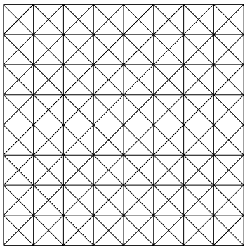
(a) $\mathcal{T}_{h}$ : $8\times 8\times 4$ mesh

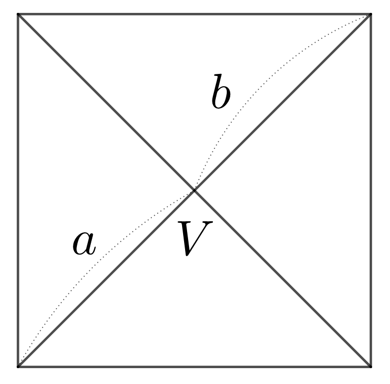
(b) $a:b=1.0005:1$

Figure 14: An example of $\mathcal{T}_{h}$ with a quasi singular vertex $\mathbf{V}$ in every squares

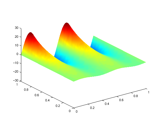
(a) $p$ over $\Omega$

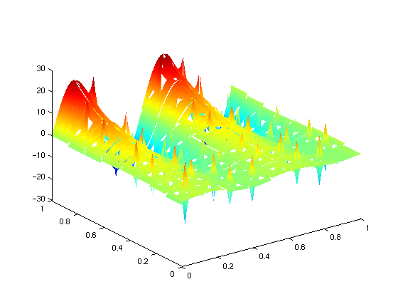
(b) $p_{h}$ over $\Omega$

Figure 15: Graphs of $p$ and $p_{h}$ solved in $8\times 8\times 4$ mesh in Figure 14

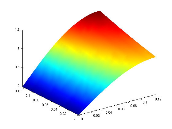
(a) $p$ over 4 triangles

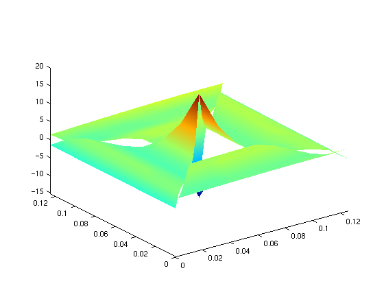
(b) $p_{h}$ over 4 triangles

Figure 16: Graphs of $p$ and $p_{h}$ over 4 triangles in $[0,1/8]^{2}$

(a) $\widetilde{p}_{h}$ over $\Omega$

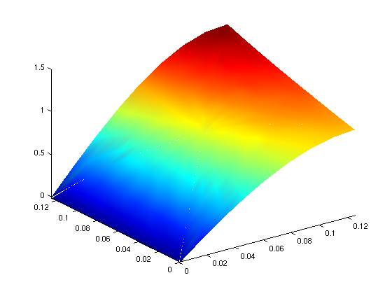
(b) $\widetilde{p}_{h}$ over 4 triangles

Figure 17: Graphs of postprocessed $\widetilde{p}_{h}$ from $p_{h}$

mesh	$|\mathbf{u}-\mathbf{u}_{h}|_{1}$	order	$\|p-p_{h}\|_{0}$	order	$\|p-\widetilde{p}_{h}\|_{0}$	order
4 x 4 x 4	8.5504E-3		2.2102E+1		5.7023E-2
8 x 8 x 4	5.4471E-4	3.9724	8.3012E-1	4.7347	2.6680E-3	4.4177
16 x 16 x 4	3.3925E-5	4.0051	2.6856E-2	4.9500	1.6624E-4	4.0044
32 x 32 x 4	2.1182E-6	4.0014	9.8863E-4	4.7637	1.0380E-5	4.0014

Table 1: Error table for meshes with quasi singular vertices as in Figure 14

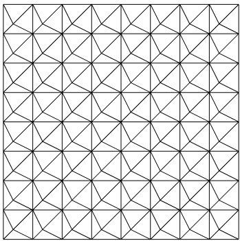
(a) $\mathcal{T}_{h}$ : $8\times 8\times 4$ mesh

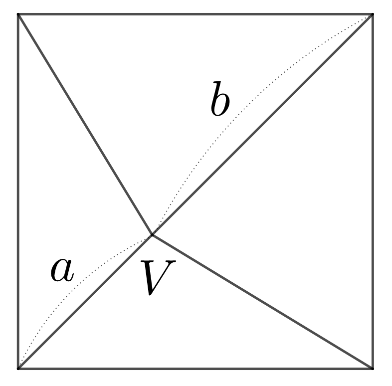
(b) $a:b=3:5$

Figure 18: $\mathcal{T}_{h}$ with no quasi singular vertex

mesh	$|\mathbf{u}-\mathbf{u}_{h}|_{1}$	order	$\|p-p_{h}\|_{0}$	order	$\|p-\widetilde{p}_{h}\|_{0}$	order
4 x 4 x 4	1.3539E-2		9.8341E-2		6.9479E-2
8 x 8 x 4	8.7627E-4	3.9496	5.6435E-3	4.1231	3.4819E-3	4.3186
16 x 16 x 4	5.4353E-5	4.0109	3.4576E-4	4.0287	2.1298E-4	4.0311
32 x 32 x 4	3.3688E-6	4.0120	2.1285E-5	4.0218	1.3114E-5	4.0216

Table 2: Error table for meshes with no quasi singular vertex as in Figure 18

References

- [1] C. Bernardi and G. Raugel, Analysis of some finite elements for the Stokes problem, Mathematics of Computation, 44 (1985), 71-79, DOI: 10.2307/2007793
- [2] D. Braess, Finite elements, Cambridge University Press, Cambridge, 2001
- [3] S. C. Brenner and L. R. Scott, The mathematical theory of finite element methods, Springer-Verlag, New York, 2nd edition, 2002
- [4] P. G. Ciarlet, The finite element method for elliptic equations, North-Holland, Amsterdam, 1978
- [5] R. S. Falk and M. Neilan, Stokes complexes and the construction of stable finite elements with pointwise mass conservation, SIAM journal of Numerical Analysis, 51 (2013), 1308-1326, DOI: 10.1137/120888132
- [6] J. Guzman and L. R. Scott, The Scott-Vogelius finite elements revisited, Mathematics of Computation, electronically published (2018), DOI: 10.1090/mcom/3346
- [7] J. N. Lyness and D. Jespersen, Moderate degree symmetric quadrature rules for the triangle, IMA Journal of Applied Mathematics, 15 (1975), 19-32, DOI: 10.1093/imamat/15.1.19
- [8] M. Neilan, Discrete and conforming smooth de Rham complexes in three dimensions, Mathematics of Computation, 84 (2015), 2059-2081, DOI: 10.1090/S0025-5718-2015-02958-5
- [9] L. R. Scott and M. Vogelius, Norm estimates for a maximal right inverse of the divergence operator in spaces of piecewise polynomials, ESIAM: M2AN, 19 (1985), 111-143, DOI: 10.1051/m2an/1985190101111
- [10] S. Zhang, On the family of divergence-free finite elements on tetrahedral grids for the Stokes equations, Preprint, University of Delaware, 2007
- [11] S. Zhang, Divergence-free finite elements On tetrahedral grids for , Mathematics of Computation, 80 (2011), 669-695, DOI: 10.1090/S0025-5718-2010-02412-3