APEX Millimeter Observations of Methanol Emission Toward High-Mass Star-Forming Cores

Abstract

We present 247-GHz molecular line observations of methanol (CH₃OH) toward sixteen massive star-forming regions, using the APEX telescope with an angular resolution of 25^′′. The sample covers a range of evolutionary states, including warm molecular cores, hot molecular cores, and ultracompact HII regions. The hot cores, all of which include UC HII regions, show rich molecular line spectra, although the strength of different species and transitions varies from source to source. In contrast, the warm cores do not show significant molecular line emission. Multiple methanol transitions are detected toward nine of the hot cores; eight of these had enough transitions to use the rotation diagram method to estimate rotational temperatures and column densities. The temperatures lie in the range 104–168 K and column densities from $3\times 10^{16}$ to $7\times 10^{18}$ cm^-2. Using the average methanol line parameters, we estimate virial masses, which fall in the range from 145 to 720 M_⊙ and proved to be significantly higher than the measured gas masses. We discuss possible scenarios to explain the chemical differences between hot cores and warm molecular cores. One of the observed methanol lines, $4_{2}-5_{1}$A⁺ at 247.228 GHz, is predicted to show class II maser emission, similar in intensity to previously reported $J_{0}-J_{-1}$E masers at 157 GHz. We did not find any clear evidence for maser emission among the observed sources; however, a weak maser in this line may exist in G345.01+1.79.

1 Introduction

Massive stars ($M>8$ M _⊙) play a fundamental role in the evolution of galaxies. The large amounts of radiation and mechanical energy they deposit into the interstellar medium can profoundly affect the star formation rate, either by initiating new star formation by compressing the interstellar gas or terminating star formation, by heating and dispersing molecular clouds. (see, e.g., Zinnecker & Yorke, 2007).

Studies show that star-forming regions (SFRs) within Infrared Dark Clouds (IRDCs, e.g., Chambers et al., 2009) contain massive cores with typical masses of $\sim 120$ M_⊙, sizes of $<$0.5 pc, densities of $\sim 10^{5}-10^{6}$ cm^-3, and temperatures of 15–30 K (e.g., Rathborne et al., 2006). While most of these massive cores show no evidence for active star formation (they are often called cold or quiescent cores; (e.g., Rathborne et al., 2006), others show bright 24 $\mu$m emission, high-excitation molecular line emission, and maser emission. These warm molecular cores (WMC) are thought to be actively forming massive stars (e.g., Garay et al., 2004; Chambers et al., 2009).

Hot molecular cores (HMC) are more-evolved objects than WMC, with higher temperatures ($>$100 K), densities ($\sim 10^{7}$ cm^-3), and luminosities ($>10^{4}$ L_⊙). They are compact ($<$0.1 pc) and have a very rich chemistry. Their molecular gas is probably heated by embedded massive (proto)stars (Kurtz et al., 2000; Cesaroni, 2005). HMC can also host energetic outflows while simultaneously undergoing infall in their outer regions (e.g., Osorio et al., 2009; Mayen-Gijon et al., 2014). The mass accretion rates in some cases may be sufficient to quench the development of HII regions (Walmsley et al., 1995; Zapata et al., 2008a; Osorio et al., 2009). Thus, it is thought that HMCs precede the development of ultracompact (UC) HII regions.

Some molecular species in HMCs show maser emission, including H₂O, H₂CO, NH₃, OH, and CH₃OH. In particular, CH₃OH  presents a complex spectrum with numerous thermal and/or maser lines. These lines are sensitive to the molecular gas conditions, allowing a detailed analysis of physical parameters. Methanol masers are also important tracers of dynamical phenomena associated with massive star formation: they are often associated with molecular outflows, disks, and shocks (Minier et al., 2005; Ellingsen, 2006, and references therein).

Methanol masers are grouped into two classes (I and II; Menten, 1991). Class I masers are typically offset from the protostellar position with the more distant masers located $\gtrsim$0.1 pc away from them (Kurtz et al., 2004); many of these masers are found to be substantially closer, however, (McCarthy et al., 2018). Class I masers are thought to be collisionally pumped (Cragg et al., 1992; Leurini et al., 2016). Class II masers are usually found very near to the protostellar position and are thought to be radiatively pumped (Cragg et al., 2005). Methanol maser surveys have shown that class II masers are exclusively associated with massive star formation regions (MSFRs) (Minier et al., 2003; Xu et al., 2008). The strongest class II masers are observed in the centimeter-wave regime, while weaker lines are detected at 3, 2, and 1 mm (Val’tts et al., 1995; Slysh et al., 1995; Zinchenko et al., 2017).

Sobolev et al. (1997) and Cragg et al. (2005) developed models to predict class II masing of methanol transitions in the 6 to 700 GHz range. Their models demonstrate that maser intensity diminishes at higher frequencies due to lesser degrees of population inversion. To constrain these models it is useful to determine which high-frequency transitions show maser emission and the relative intensities of these transitions. In the millimeter regime, one of the better maser candidates is the $4_{2}-5_{1}$ A⁺ transition at 247.228 GHz. Model 3 of Cragg et al. (2005) predicts a brightness temperature of $10^{6.2}$ K for this line, approximately the same as the brightness temperature of known class II masers at 157 GHz (Slysh et al., 1995) and about a factor of 5 lower than the brightness temperature of another known Class II maser line, $3_{0}-4_{-1}$ A⁺ at 107 GHz (Val’tts et al., 1995). This model predicts a brightness temperature ratio for the 6.7 and 247.2 GHz masers of $10^{4.3}$, and hence the predicted ratio of 6.7/247.2 GHz flux densities is about 15. Because many 6.7 GHz masers show flux densities of hundreds of Janskys, one can expect that masers at 247.2 GHz will have intensities high enough to be easily detected.

Table 1: Observed Sources

Source	Short	$\alpha\;$(J2000)	$\delta\;$(J2000)	VLSR	Distance	$L_{\rm bol}$
	Name	${}^{h}\;{}^{m}\;{}^{s}$	${}^{o}\;{{}^{\prime}}\;{{}^{\prime\prime}}$	(km s-1)	(kpc)	($10^{5}$ ${\rm L}_{\odot}$)	Commentsa	Refs.
G345.01+1.79	G345.01	$16^{h}56^{m}47.6^{s}$	$-$40 14 26	$-$14	2.4	0.21	HMC+UC HII	12
G351.417+0.645	N6334 F	17 20 53.4	$-$35 47 01	$-$10.5	1.3b	1.5	HMC+UC HII	11,14
G351.446+0.659	N6334 I(N)	17 20 55.0	$-$35 45 05	$-$3	1.3b	0.01	HMC+UC HII	1,14
G351.776-0.537	I17233	17 26 43.0	$-$36 09 15	$-$3	1.2	0.14	HMC+UC HII	2,3,13
G9.621+0.196	G9.62	18 06 14.7	$-$20 31 32	$-$3	5.2b		HMC+UC HII	16
G10.47+0.03	G10.47	18 08 38.2	$-$19 51 49	+68	8.5b	7.0	HMC+UC HII	4,5
G10.62–0.38	G10.62	18 10 28.7	$-$19 55 49	$-$3	5.0b	9.2	HMC+UC HII	5,6
G20.08-0.14N	G20.08N	18 28 10.3	$-$11 28 48	+42	12.3	6.6	HMC+UC HII	7
G24.33+0.11MM1	G24.33	18 35 08.1	$-$07 35 04	+53	3.8	0.4	WMC	10
G28.53–0.25MM2	G28.53	18 44 15.7	$-$03 59 41	+87	5.7	0.005	WMC	10
G29.96–0.02	G29.96	18 46 03.9	$-$02 39 21	+97	5.2b	4.3	HMC+UC HII	8,5
G30.97–0.14MM1	G30.97	18 48 22.0	$-$01 48 27	+79	5.1	0.04	WMC	10
G31.97+0.07MM1	G31.97	18 49 36.6	$-$00 45 45	+97	5.1	0.36	WMC	10,5
G34.26+0.15	G34.26	18 53 18.5	+01 14 57	+58	3.7	5.2	HMC+UC HII	9
G35.204-1.738	W48	19 01 46.2	+01 13 42	+45.7	3.27b	0.08	UC HII	15
G45.07+0.13	G45.07	19 13 22.0	+10 50 53	+60	8.0b	11.0	HMC+UC HII	4,5

Note. — Units of right ascension are hours, minutes, and seconds, and for declination are degrees, arcminutes, and arcseconds. Positions, V_lsr, and luminosities are taken from the cited references. (a) Hot molecular cores (HMC), all of them showing ultracompact HII regions (UC HII), and warm massive cores (WMC) associated with infrared dark clouds. (b) trigonometric parallax distance, taken from (Reid et al., 2014, and references therein). Otherwise, the distance is kinematic and taken from the cited references.

References— (1) Chibueze et al. (2014); (2) Leurini et al. (2011); (3) Fáundez et al. (2004); (4) Pandian et al. (2008); (5) Reid et al. (2014); (6) Sollins et al. (2005); (7) Galván-Madrid et al. (2009); (8) Beuther et al. (2007); (9) Mookerjea et al. (2007); (10) Rathborne et al. (2006); (11) Hunter et al. (2018); (12) Lumsden et al. (2013); (13) Zapata et al. (2008b); (14) Brogan et al. (2016) (15) Rygl et al. (2014) (16) Liu et al. (2017)

An additional advantage of selecting the 247.2 GHz line for the observations is the location of its energy levels. The upper level of the $4_{2}-5_{1}$ A⁺ transition belongs to the $K=2\;$A⁺ ladder while the lower level belongs to the $K=1\;$ A⁺ ladder. Little is known about masers in $K=2\rightarrow K=1$ transitions of methanol A. Only three regions, W3(OH), NGC6334F, and NGC7538, have been found to show maser emission in the $9_{2}-10_{1}$ A⁺ transition at 23 GHz (Cragg et al., 2004, and references therein). A fourth 23 GHz methanol maser has recently been reported in G358.93$-$0.03, but it has not yet been confirmed by interferometric observations (O. Bayandina, personal communication). Slysh et al. (1995) detected the 156.1 GHz $6_{2}-7_{1}$ A⁺ transition in only one source, W3(OH), and reported a weak, broad line, which may contain a narrow maser component. Although these masers are fairly rare, information about their intensities will help to constrain maser models.

To test the predictions of the Sobolev/Cragg model, we observed 16 MSFRs associated with WMCs, UC HII, or HMC+UC HII-regions, using the APEX antenna. The latter sources are HMC that are closely associated with UC HII regions. Fifteen of the sources (all but G28.53) show methanol maser emission at 6.7 GHz, with peak fluxes ranging from 2 to $\sim 5000$ Jy, and a median value of 36 Jy. In addition, G345.01+1.79 and W48 are the only two masers at 157 GHz detected by Slysh et al. (1995) in the southern hemisphere; these masers also emit at 107 GHz (Val’tts et al., 1999); G9.62+0.19 is the strongest maser at 6.7 GHz, according to Menten (1991) and shows maser emission at 107 GHz (Val’tts et al., 1999), and NGC6334F presents strong maser emission at 23 GHz (Cragg et al., 2004) and 107 GHz (Val’tts et al., 1999). Thus, our target list includes the most probable candidates for detecting masers in the $4_{2}-5_{1}$ A⁺ transition, achievable for APEX.

Our APEX observations and the reduction procedures are described in Sect. 2. Results and discussion are presented in Sect. 3, and we make some concluding remarks in Sect. 4.

2 Observations and data reduction

In Table 1 we list the observed sources. The sample is comprised of four WMC, one UC HII region and eleven HMC + UC HII-regions. The WMCs were selected from a list of cores associated with IRDCs (Rathborne et al., 2006). These four sources have masses (determined from 1.2 mm dust continuum emission) above 400 M_⊙, present 4.5 $\mu$m emission (often associated with shocks and outflows), strong 8.0 $\mu$m emission, class II CH₃OH maser emission at 6.7 GHz and class I maser emission at centimeter wavelengths. The HMC and UC HII-regions were selected from the literature and are well-known MSFRs with luminosities greater than $10^{4}$ L_⊙ and all show class II methanol maser emission.

The observations were made using the APEX 12-m telescope at Llano de Chajnantor in the Atacama desert of Chile (Chilean time project C-086.F-0667B-2010 and Swedish time project O-0100.F-9307A-2017). The first observing run was performed during 2010 August–December. We used the SHFI APEX-1 receiver (Vassilev et al., 2008) and the Fast Fourier Transform Spectrometer (FFTS) configured with two units, each with a bandwidth of 1 GHz and 8192 channels. We overlapped the units to achieve 1.8 GHz total bandwidth, centered at 247228.73 MHz (1.21 mm wavelength) which is the rest frequency of the CH₃OH (4${}_{2}-5_{1}$ A⁺) line. The channel width was 0.15 km s^-1, and the total velocity coverage was 2200 km s^-1. At the observing frequency of 247 GHz the APEX forward efficiency is 0.95, the main beam efficiency is $\eta_{\rm mb}=0.75$, and the primary beamwidth is $\theta_{\rm FWHM}=25$.^′′2. We made single-pointing, beam-switched observations of each source for 10 minutes duration (on-source), achieving a typical rms of 45 mK. We used RAFGL 2135 and NGC 6302 as pointing sources at different epochs.

Table 2: Parameters of some detected molecular lines

Species	Transition	Frequency	$E_{u}$
		(GHz)	(K)
HC3N	$27-26~{}1v7~{}l=1f$	246.5607	486
HC3N	$27-26~{}2v7~{}l=0$	247.1146	807
HC3N	$27-26~{}2v7~{}l=2f$	247.2099	811
CH3OH	$21_{3}A^{-}-21_{2}$A+	245.2235	586
CH3OH	$20_{3}A^{-}-20_{2}$A+	246.0749	537
CH3OH	$19_{3}A^{-}-19_{2}$A+	246.8735	490
CH3OH	$16_{2}-15_{3}$E	247.1619	338
CH3OH	$4_{2}-5_{1}$A+	247.2287	70
CH3OH	$18_{3}A^{-}-18_{2}$A+	247.6110	446
CH3OH	$12_{-2}-13_{-3}$E  $v_{t}=1$	247.8402	545
CH3OH	$23_{1}-23_{0}$E	247.9681	661
CH3OH	$17_{3}A^{-}-17_{2}$A+	248.2825	405
CH3OH	$16_{3}A^{-}-16_{2}$A+	248.8855	365
SO2	$15_{2}-15_{1}$	248.0574	119
SO2	$31_{9}-32_{8}$	247.1697	654
34SO	$5_{3}-5_{2}$	247.4403	35
34SO	$4_{1}-4_{2}$	246.6861	30
CH3CH2CN	$28_{1}-27_{1}$	248.0425	176
CH3CH2CN	$27_{3}-26_{3}$	246.5487	174
CH3CH2CN	$28_{2}-27_{2}$	246.4219	177

Several of the more promising sources for maser detections at 247 GHz were not scheduled during the first run. Therefore, we performed additional observations in August 2017. We used the APEX-1 receiver and the Extended Fast Fourier Transform Spectrometer (XFFTS) configured with both spectral units, overlapped by 1000 MHz, giving a usable bandwidth of $\sim$ 4 GHz, and allowing the search for a number of additional molecular transitions. The observational technique and the time per source were the same as in the first observing run.

The data reduction was done with the CLASS software package. First, we inspected the raw data to eliminate any bad spectra in either of the FFTS units. The spectra were then combined into a single spectral window. The width of the window was 1.8 GHz for the 2010 data and 4 GHz for the 2017 data. To fit a baseline, we selected windows avoiding any obvious line emission and fitted a polynomial of order 3 or less. The data were smoothed by 6 channels (i.e., averaged without overlap) to obtain a velocity resolution of 0.9 km s^-1 (0.74 km s^-1 for the 2017 data) and an rms of 0.016–0.018 K in the final spectra, which we used for further analysis. We converted the antenna temperature, $T_{\rm A}^{*}$, to main-beam brightness temperature, $T_{\rm mb}$, through $T_{\rm mb}=T_{\rm A}^{*}/\eta_{\rm mb}$.

Figure 1: Wide-band continuum-free spectra taken with APEX in 2010.

Figure 1: (continued)

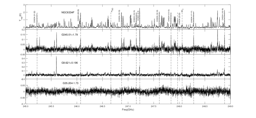
Figure 2: Wide-band continuum-free spectra taken with APEX in 2017. We label several CH₃OH lines, the SO₂ line at 248.05 GHz, and the ³⁴SO line.

3 RESULTS and DISCUSSION

3.1 Detection of molecular line emission

In Figures 1 and 2 we show the spectra of the sixteen sources. In Table 2 we list some physical characteristics of the major lines we detected. We used the SPLATALOGUE website to identify the main lines in the spectra. We note that the large number of emission lines produces blending of some lines in sources such as N6334F, I17233, G34.26, and G10.47 (see Figures 1 and 2), which complicates the line identification. High angular resolution ALMA observations would be more adequate for this purpose, and also to trace the gas dynamics within the cores.

Four of the 12 sources that harbor HMCs and/or UC HII, NGC6334F, I17233, G10.47, and G34.26, contain numerous emission lines from oxygenated, nitrogenated, and sulfurated species, along with their isotopomers. Distinct molecular species detected include HC₃N, CH₃OH, SO₂, ³³SO₂, ³⁴SO, CH₃OCHO, CH₂CHCN and CH₃CH₂CN. The G29.96 and G345.01 HMC+UC HII regions show less-rich spectra, but nevertheless present emission in a number of high-energy lines. The spectra of NGC 6334 I(N) and G9.62 are even more line–poor than those of G29.96 and G345.01. G10.62, G20.08M, G35.204, and G45.07 show only a few lines in their spectra. We note that all the above are HMCs or HMC + UC HII-regions. The four warm cores, G31.97MM1, G28.53MM2, G24.33MM1, and G30.97MM1, show very little molecular line emission.

3.2 Comparison between sources

I17233, NGC6334F, G34.26, and G10.47 show notably richer spectra than other HMCs such as G345.01, NGC 6334 I(N), G9.621, G10.62, G20.08N, G29.96, and G45.07. This is consistent with the results of Hernández-Hernández et al. (2014), who studied a sample of 17 hot cores in methyl cyanide lines and found that the CH₃CN line intensities, and hence the column densities, in G10.62 and G45.07 are much lower than those in I17233 and G10.47.

In addition, we see differences in the emission of some molecular lines within these regions. For example, NGC 6334 I(N) and G10.62 show strong emission from the CH₃OH $4_{2}-5_{1}A^{+}$ line compared to G45.07 and G20.08N. On the other hand, G45.07 and G10.62 show strong emission in SO₂ (at 248.05 GHz) and ³⁴SO (at 246.66 GHz), while G29.96, NGC 6334 I(N), and G20.08N are very weak in these lines. In any case, for all these sources, we detect the $4_{2}-5_{1}A^{+}$ CH₃OH and $15_{1}-15_{2}$ SO₂ transitions, which have excitation temperatures of 70 and 120 K, respectively. Differences in the number of transitions and which molecules are in emission have been reported toward other MSFRs, such as the Orion hot core and W3(OH)–TW (Wyrowski et al., 1999; Qin et al., 2015). Significant differences in the number and intensity of molecular lines in different SFRs was found by Hatchell et al. (1998), who divided the observed sources into line-rich and line-poor. An extensive systematic study of more than 100 SFRs by Giannetti et al. (2017) also showed a similar picture. The differences have variously been explained as the result of different physical conditions, different composition of ice-mantles on dust grains, or different evolutionary stages (Choudhary et al., 2015; Beuther et al., 2009).

Table 3: Observed Parameters of CH₃OH lines

Source	$T_{\rm mb}$	FWHM	$\int T_{\rm mb}\Delta V$	VLSR
Transition	(K)	(km s-1)	(K km s-1)	(km s-1)
G345.01+1.79
(21–21)	0.08	$5.34\pm 0.60$	$0.45\pm 0.04$	-12.30
(20–20)	0.11	$6.70\pm 0.50$	$0.77\pm 0.05$	-13.56
(19–19)	0.12	$5.20\pm 0.36$	$0.64\pm 0.04$	-13.31
(16–15)	0.11	$5.02\pm 0.48$	$0.58\pm 0.05$	-13.34
(4–5)	0.32	$4.11\pm 0.18$	$1.41\pm 0.05$	-13.00
	0.08	$2.48\pm 0.59$	$0.21\pm 0.05$	-17.62
(18–18)	0.12	$6.01\pm 0.53$	$0.79\pm 0.06$	-13.53
(12–13)	0.08	$7.49\pm 1.84$	$0.65\pm 0.06$	-13.21
(23–23)	0.05	$4.77\pm 1.08$	$0.25\pm 0.05$	-13.76
(17–17)	0.11	$5.61\pm 0.49$	$0.66\pm 0.05$	-13.32
(16–16)	0.13	$5.49\pm 0.37$	$0.74\pm 0.05$	-13.20
NGC6334F
(21-21)	1.81	$5.60\pm 0.09$	$10.75\pm 0.15$	-7.06
(20-20)	2.00	$6.38\pm 0.05$	$13.57\pm 0.09$	-7.78
(19-19)	2.11	$5.08\pm 0.05$	$11.40\pm 0.10$	-7.65
	0.42	$4.69\pm 0.11$	$2.11\pm 0.05$	-3.03
(16-15)	1.92	$6.03\pm 0.09$	$12.31\pm 0.16$	-7.76
(4-5)	2.56	$5.56\pm 0.06$	$15.13\pm 0.15$	-7.81
(18-18)	2.10	$5.14\pm 0.08$	$11.46\pm 0.12$	-7.82
	0.36	$4.14\pm 0.16$	$1.57\pm 0.06$	-3.35
(12-13)	1.95	$5.49\pm 0.06$	$11.41\pm 0.15$	-7.09
(23-23)	1.20	$5.31\pm 0.05$	$6.79\pm 0.05$	-7.15
(17-17)	2.16	$5.36\pm 0.05$	$12.30\pm 0.11$	-7.96
	0.18	$2.62\pm 0.22$	$0.51\pm 0.04$	-4.44
(16-16)	2.13	$5.30\pm 0.05$	$12.04\pm 0.10$	-8.22
	0.22	$3.03\pm 0.16$	$0.74\pm 0.04$	-4.53
N6334 I(N)
(16-15)	0.09	5.83$\pm$0.822	0.50$\pm$0.073	-3
(4-5)	0.42	4.46$\pm$0.188	1.88$\pm$0.680	-3
(18-18)	0.13	6.07$\pm$0.841	0.73$\pm$0.096	-3
I17233
(19-19)	0.49	8.73$\pm$0.639	4.58$\pm$0.296	-5
(16-15)	0.47	9.47$\pm$0.440	5.10$\pm$0.206	-5
(4-5)	0.68	8.60$\pm$0.255	6.22$\pm$0.156	-4
(18-18)	0.60	8.28$\pm$0.176	5.68$\pm$0.100	-5
(23-23)	0.12	6.89$\pm$1.256	0.94$\pm$0.149	-5
(12-13)	0.21	8.18$\pm$0.753	1.86$\pm$0.160	-4
G9.62
(21-21)	0.07	$6.99\pm 0.92$	$0.52\pm 0.06$	3.78
(20-20)	0.06	$5.29\pm 0.97$	$0.36\pm 0.05$	3.35
(19-19)	0.11	$4.89\pm 0.43$	$0.56\pm 0.04$	3.63
(16-15)	0.10	$5.68\pm 0.51$	$0.64\pm 0.05$	3.37
(4-5)	0.22	$6.03\pm 0.23$	$1.40\pm 0.05$	3.68
(18-18)	0.11	$6.08\pm 0.52$	$0.71\pm 0.06$	3.11
(12-13)	0.07	$6.51\pm 0.74$	$0.48\pm 0.05$	2.67
(17-17)	0.14	$6.27\pm 0.50$	$0.90\pm 0.06$	3.21
(16-16)	0.16	$5.65\pm 0.30$	$0.98\pm 0.05$	3.73
G10.47
(19-19)	0.65	8.98 $\pm$0.727	6.21$\pm$0.442	+66
(16-15)	0.54	10.89$\pm$0.891	6.36$\pm$0.405	+66
(4-5)	0.65	10.10$\pm$0.685	7.00$\pm$0.382	+66
(18-18)	0.68	9.90 $\pm$0.887	7.10$\pm$0.566	+65
(23-23)	0.29	10.08$\pm$1.651	3.13$\pm$0.378	+66
(12-13)	0.41	9.97 $\pm$0.911	4.41$\pm$0.345	+66
G10.62
(4-5)	0.29	7.65$\pm$0.495	2.28$\pm$0.126	-3
G20.08N
(4-5)	0.07	5.44$\pm$1.134	0.41$\pm$0.078	+42
G29.96
(19-19)	0.19	6.10$\pm$0.506	1.17$\pm$0.081	+98
(16-15)	0.16	6.61$\pm$0.543	1.13$\pm$0.080	+98
(4-5)	0.29	6.09$\pm$0.421	1.61$\pm$0.082	+98
(18-18)	0.19	7.37$\pm$0.856	1.34$\pm$0.109	+98
(23-23)	0.06	3.09$\pm$1.101	0.22$\pm$0.066	+98
(12-13)	0.14	4.67$\pm$0.690	0.58$\pm$0.076	+98
G31.97MM1
(4-5)	0.12	4.46$\pm$0.616	0.56$\pm$0.065	+97
G34.26
(19-19)	0.78	6.97$\pm$0.332	5.40$\pm$0.233	+59
(16-15)	0.69	6.28$\pm$0.278	4.73$\pm$0.180	+59
(4-5)	0.86	6.44$\pm$0.222	6.22$\pm$0.182	+59
(18-18)	0.82	7.67$\pm$0.623	6.22$\pm$0.462	+59
(23-23)	0.28	7.07$\pm$0.841	2.30$\pm$0.220	+58
(12-13)	0.49	5.55$\pm$0.661	2.00$\pm$0.194	+59
W48
(4-5)	0.04	4.54$\pm$0.993	0.19$\pm$0.038	+42.34

3.3 Null detection of maser emission?

The $4_{2}-5_{1}$ A⁺ methanol line at 247.2 GHz is a candidate to show maser emission (Sobolev et al., 1997; Cragg et al., 2005). However, we detected only broad lines at this frequency, ranging from 4.5 to 10.1 km s^-1. The similarity of the $4_{2}-5_{1}$ A⁺ line profiles to the other thermal methanol lines (see Fig. 3) suggests that the former transition is also thermal. In addition, rotation diagrams constructed for eight sources (see below) show that the ratios of different line intensities correspond to local thermodynamic equilibrium (LTE). Thus, in most cases, the emission in the 247.2 GHz line is probably thermal.

A possible exception is the spectral feature at $-17.62$ km s^-1 in G345.01 (see Table 3 and Fig. 3). The origin of this feature is uncertain. On the one hand, similar, but less prominent features can be seen in the spectra of other lines (Fig. 3). Maser velocities in this object are usually more negative than $-20$ km s^-1 (e.g. Ellingsen et al., 2012). These facts indicate that the emission at $-17.62$ km s^-1 may be thermal. On the other hand, Krishnan et al. (2013) detected a weak methanol maser in the 19.9 GHz $2_{1}-3_{0}$ E line in this source precisely at $-17.5$ km s^-1, and Ellingsen et al. (2018) found weak maser emission in the $7_{-2}-8_{-1}$ E, $6_{2}-5_{3}{\rm A}^{-}$, and $6_{2}-5_{3}{\rm A}^{+}$ Class II transitions at 37.7, 38.3, and 38.5 GHz at around $-17$ km s^-1 (in addition to stronger emission at velocities $<-20$ km s^-1). Interferometric observations with ALMA or the SMA could help establish the origin of this feature.

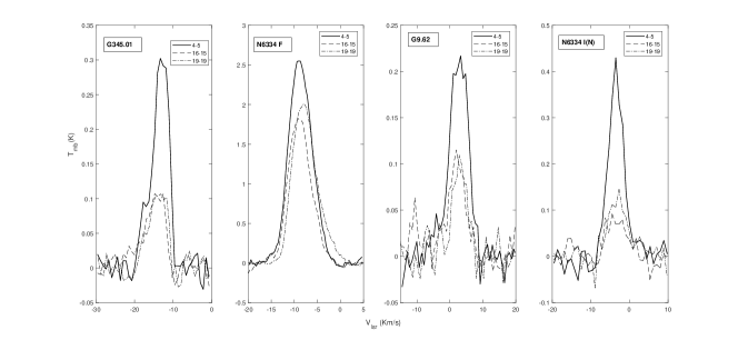
Figure 3: Spectra of methanol lines of G345.01, NGC6334F, G9.62, and NGC6334I(N). Thick solid lines shows the profiles of the $4_{2}-5_{1}$A⁺ line, thin dashed lines, profiles of two other methanol lines detected in these sources.

G10.62, G31.97MM1, and NGC 6334 I(N) show fairly strong $4_{2}-5_{1}{\rm A}^{+}$ lines, while other methanol lines are weak or absent. Because the 247.2 GHz lines are broad in these sources, most likely they are thermal and the weakness/absence of other methanol lines means that the gas is too cold to excite them. Note that the upper energy level of the $4_{2}-5_{1}{\rm A}^{+}$ transition corresponds to 70 K, while the upper levels of the other methanol lines in our passband range from 338 to 661 K.

Because our source list contained the most promising sources from the viewpoint of detecting masers in the $4_{2}-5_{1}$ A⁺ transition (see Section 1), we conclude that maser emission at 247.2 GHz, comparable in intensity with that at 157 GHz or 107 GHz, either never arises, or only arises in very rare cases; hence, the maser regime described by Model 3 of Cragg et al. (2005) is unusual for Class II masers.

Model 3 is characterized by a low gas kinetic temperature. While the dust, whose radiation inverts the Class II transitions, has a temperature of 175 K in this model, similar to those in other models, the gas temperature here is only 30 K. This is the lowest gas temperature model of Cragg et al. (2005). The model also predicts bright masers at 19.9 and 37.7 GHz, as well as weaker masers at 38.3, and 38.5 GHz — which are detected in G345.01. The second lowest gas temperature model (Model 7) also predicts a fairly high brightness temperature at 247.2 GHz, of $10^{5.6}$ K. Note that the latter model does not predict bright masers at 157 GHz. Other models have gas temperatures of 120 K and higher and do not predict substantial emission at 247.2 GHz. Thus, masers at 247.2 GHz may exist only in cold gas permeated by much hotter radiation. Our results show that such conditions are unusal for star-forming regions, although they may occur in rare cases, such as G345.01+1.79.

3.4 Methanol detections in our sample

CH₃OH is a common molecule in MSFRs, with abundances of order $10^{-9}$ in the cold gas phase (e.g. van der Tak et al., 2000). Its formation is thought to occur by grain-surface chemical reactions during an early, cold stage in massive cores. Gas-phase production of CH₃OH at temperatures $<100$ K is mainly through radiative association of CH${}_{3}^{+}$ and H₂O and subsequent dissociative recombination of the resulting CH₃OH${}_{2}^{+}$ ion. This pathway is relatively inefficient, however, yielding abundances of only $\sim 10^{-11}$ relative to H₂ (Geppert et al., 2006). Thus, gas-phase chemistry cannot account for the observed abundances and grain surface chemistry is invoked to reach the larger observed abundances (e.g., Garrod et al., 2007). Subsequent to its formation on grain surfaces, methanol sublimates as the grains are heated during the star formation process, either by radiation (e.g., van der Tak et al., 2000) or from shocks (Bachiller et al., 1995, 1998; Garay et al., 2002; Kalenskii et al., 2007). Thus, the presence or absence of methanol emission, and its abundance, are expected to depend on the evolutionary state of the region.

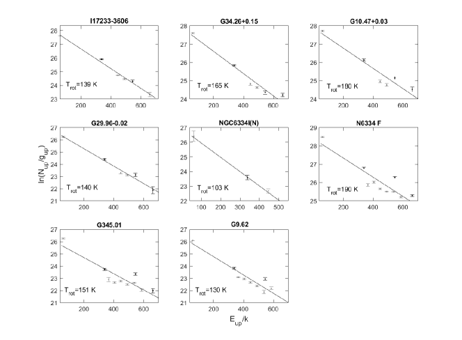
Figure 4: Rotation diagrams for methanol emission from eight sources. The solid lines show the linear fits to all the data points in the plots. The grey circles show A-methanol levels and the black circles show E-methanol levels.

Figure 5: Model rotation diagram for A and E methanol. The filled circles show A-methanol levels and the open stars show E-methanol levels.

The sixteen MSFRs we observed are in different evolutionary stages. Table 1 indicates the general stage of each region, ranging from young (warm core), to advanced (hot molecular core plus UC HII region). We note that the HMC + UC HII category also contains a range of evolutionary states: in some cases the UC HII regions are well-developed (e. g. G34.26; Wood & Churchwell, 1989) while in other cases they appear to be nascent (e. g. NGC 6334 I(N); Hunter et al., 2014). Of the four warm cores, only one (G31.97MM1), shows methanol emission.

Among the eleven hot molecular cores, there are notable differences in their methanol emission. Four of the HMCs (I17233, NGC6334F, G34.26, and G10.47) are very rich in lines of methanol and other molecules, showing at least six methanol transitions. Five other objects, G345.01, NGC 6334 I(N), G9.621, G10.62, and G29.96, have weaker lines of methanol and other molecules. The remaining two HMCs (G45.07 and G20.08N) show almost no methanol emission — only a weak detection of the $4_{2}-5_{1}{\rm A}^{+}$ line in G20.08N.

3.5 Rotation diagram analysis

The CH₃OH transitions we detect can be used to estimate the rotation temperature and column density of the gas via a rotation diagram (RD) analysis (e. g. Turner, 1991). This method assumes that multiple transitions of a molecular species are optically thin and that the molecules are in LTE; that is, the ratios of all upper-level populations correspond to a single rotational temperature. No background radiation is considered, and uniform temperature and density are assumed. If the molecular transitions are thermalized by collisions, the rotation temperature will closely approximate the gas kinematic temperature.

Thus, the velocity-integrated main-beam brightness temperature, $\int T_{\rm mb}dv$, is related to the species column density in the upper level, $N_{\rm u}$, by

$${\rm ln}\left(\frac{3k\int T_{\rm mb}dv}{8\pi^{3}\mu^{2}\nu{\rm S}}\right)={\rm ln}\left(\frac{N_{u}}{g_{u}}\right)={\rm ln}\left(\frac{N_{\rm tot}}{Q_{\rm rot}}\right)-\frac{E_{\rm u}}{kT_{\rm rot}}$$ (1)

where $\nu$ is frequency, $\mu$ the dipole moment, S is the line strength, $g_{\rm u}$ is the total degeneracy of the upper state, $N_{\rm tot}$ is the column density of the molecule in all states, and $E_{\rm u}$ is the energy of the upper level. For the spectroscopic parameters we used the values from the Cologne catalog (Müller et al., 2001). The partition functions of methanol, $Q_{\rm rot}$, that depend on temperature, were derived from the catalog values. The catalog provides partition functions for a discrete sample of temperatures $T_{\rm cat}$; hence we had to interpolate between the catalog values to obtain the numerical results appropriate for our temperatures. To calculate $Q_{\rm rot}$ for a temperature $T_{\rm rot}$, we used the catalog value of the partition function for $T_{\rm cat}$ that is closest to $T_{\rm rot}$, and multiplied it by $(T_{\rm rot}/T_{\rm cat})^{1.5}$.

Equation 1 is a linear equation with slope ($-1/T_{\rm rot}$) and intercept ln($N_{\rm tot}/Q_{\rm rot}$). The rotation diagram is the plot of ln($N_{u}/g_{u}$) versus $E_{\rm u}/k$ for each molecular transition. The temperature and column density are then determined via a linear least-squares fit. As we use beam-averaged radiation temperatures the derived column densities are also beam-averaged.

We label in Figures 1 and 2 the six to ten CH₃OH transitions used in the linear fit. Also labeled are the SO₂ and ³⁴SO transitions. The resulting CH₃OH rotation diagrams for the nine sources where three or more methanol lines are detected are shown in Figure 4. The rotational temperatures obtained range from 104 to 190 K, and column densities from $1.8\times 10^{15}$ to $3.2\times 10^{16}$ cm^-2; the values are listed in Table 4. These column densities, of order $10^{15}$–$10^{16}$ cm^-2, assume a source size equal to the beam size of 25^′′. More realistic source sizes, taken from the literature, suggest column densities about two orders of magnitude higher, ranging from $3.3\times 10^{16}$ to $7.0\times 10^{18}$ cm^-2. The fact that for each source the positions of all points can be fitted by a single line corresponding to a temperature higher than 100 K demonstrates that in all nine sources, methanol emission is dominated by hot components in all observed lines, including $4_{2}-5_{1}{\rm A}^{+}$.

Note that a hot component of methanol emission in N6334F, N6334I(N), I17233, G10.47, and G34.26 have been analysed by Giannetti et al. (2017) using high-energy 7–6 methanol lines at $\sim 338$ GHz. Our temperatures are roughly in agreement with those obtained by Giannetti et al. (2017) for all sources except N6334I(N), where our temperature is lower by a factor of 1.7. Note that the rotational temperature for this source was determined using only three lines with the lowest energy levels in our sample, which may affect the result. The temperature of 179.6 K, obtained by Giannetti et al. (2017) using a larger number of lines is probably more correct than our temperature.

To determine molecular column densities in hot cores from the results of single-dish observations, hot core sizes are necessary. While Giannetti et al. (2017) determined hot core source sizes indirectly, by fitting the observed line intensities, we relied upon sizes taken from the literature; these were measured directly, but using dust or molecules other than methanol. The sizes we use for G34.26 and N6334I(N) are significantly larger (2.4 and 6.1 times, respectively), and column densities are 4.5 and 49 times lower than the Giannetti et al. values. Both of these methods to obtain source sizes have obvious shortcomings, interferometric observations of high-energy methanol lines are necessary to correctly determine methanol column densities.

Methanol is thought to form on grain surfaces via a sequence of hydrogenation reactions:

CO$\;\rightarrow\;$HCO$\;\rightarrow\;$H₂CO$\;\rightarrow\;$CH₃O$\;\rightarrow\;$CH₃OH.

Watanabe et al. (2004) and Hidaka et al. (2004) found that the efficiency of this process depends on both the dust temperature and the composition of the grain surface. Considering pure CO, as well as CO-H₂O and CO-H₂CO mixtures for the surface layer, they report that CH₃OH production can be relatively efficient for dust temperatures up to about 20 K. The hydrogenation efficiency dropped markedly above this temperature.

The initial A and E methanol abundance ratio, [A]/[E], also depends on the dust temperature (e. g. Wirström et al., 2011). It is about 1.4 for a dust temperature of 10 K, tending toward unity with increasing temperature; it is nearly unity at temperatures of 20 K and above. There are no allowed radiative or collisional transitions between A and E methanol, so these processes cannot alter the initial [A]/[E] ratio. Proton exchange reactions with H${}^{+}_{3}$ and HCO⁺ can in principle equalize the A and E methanol abundances, but these reactions are quite slow (e. g. Wirström et al., 2011); hence the initial [A]/[E] ratio should be preserved.

An over-abundance of A methanol was found in dark clouds by Friberg et al. (1988), but the situation in massive star formation regions is still uncertain. Wirström et al. (2011) determined [A]/[E] ratios in seven MSFRs; in only two of these were the ratios consistent with low formation temperatures (10 and 16 K). For a sample of Extended Green Objects, Chen et al. (2013) found a mean [A]/[E] ratio of 1.66, which is consistent with a methanol formation temperature lower than 10 K. However, the ratios for the individual sources from their sample range between 0.57 and 2.73.

We note that Chen et al. (2013) assumed LTE in their analysis. They built rotation diagrams using both A-type and E-type lines of the $2_{K}-1_{K}$ series, and then, using the derived rotational temperature, calculated methanol column densities for each A-type and E-type transition. Finally, they averaged column densities for A and E transitions separately and used the average column densities to calculate the [A]/[E] ratios.

However, methanol energy levels are rarely thermalized in the ISM (e. g. Kalenskii & Kurtz, 2016) and neglecting deviations from LTE can lead to erroneous [A]/[E] ratios. To demonstrate this, we built a model rotation diagram applying LVG intensities of the same $2_{K}-1_{K}$ methanol lines as used by Chen et al. (2013). The LVG calculations were performed with the RADEX code (van der Tak et al., 2007) for equal abundances of A and E methanol, with the gas temperature set to 30 K and the density to $3\times 10^{5}$ cm^-3. The resulting diagram is shown in Figure 5. The filled circles show A-methanol lines, while the open stars represent E-methanol lines. Note that the points do not lie on a single straight line, thus demonstrating a notable deviation from LTE. The points corresponding to A-methanol transitions are located above the approximating line, while the points corresponding to E-methanol transitions fall either on the line or below it. This means that if we assume LTE when estimating the column densities of A and E methanol, the former value will be higher than the latter one. The method used by Chen et al. (2013) yields [A]/[E] equal to 2.1.

Thus, neglecting deviations from LTE can lead to erroneous results. Unfortunately we could not analyze our results with RADEX. This code uses the LAMDA molecular database which is limited to methanol transitions between levels with $J\leq 15$. The complete solution of how to correctly determine the [A]/[E] ratio requires a special study and is beyond the scope of the present paper. Kalenskii & Shchurov (2016) used a combination of the rotation diagram method and statistical equilibrium calculations to estimate the abundances of A and E methanol in the massive star formation region L379 IRS1. The abundances in that case proved to be equal.

Inspection of Figure 4 shows that the points corresponding to both A and E methanol are well-fit by the same straight line for I17233, G34.26, G29.96, and N6334I(N). The natural explanation of this is as follows: (a) methanol level populations are in LTE; and (b) the abundances of the two species in our source sample are approximately equal. In the remaining five sources, the points corresponding to methanol E lie slightly above the points corresponding to methanol A. We believe that this is an excitation effect since there is no way to make E methanol more abundant than A methanol. These results assume that either the composition of grain mantles allows methanol formation at temperatures about 20 K or higher or that some process(es) can equalize gas-phase A and E methanol abundances faster than the proton exchange reactions studied by Wirström et al. (2011).

3.6 Discussion

The methanol lines in our passband are listed in Table 2. Nine of these lines have upper-level energies above 330 K and are detected only in very hot regions. Therefore it is not surprising that the strongest emission in these lines was detected in the most prominent hot cores of our sample. Rotation temperatures of about 130 K and higher (see Table 4) confirm that the methanol emission in these lines arises from hot cores.

Using source sizes from the literature and beam-averaged methanol column densities from our rotation diagram analysis (see Table 4), we obtain methanol column densities corrected for beam dilution. We use a beam dilution factor $\eta_{bd}=\theta_{s}^{2}/(\theta_{b}^{2}+\theta_{s}^{2})$, where $\theta_{b}$ is the FWHM of the APEX beam and $\theta_{s}$ is the source size. In this way, methanol column densities vary from $3.3\times 10^{16}$ cm^-2 for NGC 6334 I(N) to $7.0\times 10^{18}$ cm^-2 for G10.47. Column densities of H₂ for IRAS17233 and G10.47 were reported by Hernández-Hernández et al. (2014); using their values, we obtain methanol abundances of $0.5\times 10^{-7}$ for IRAS17233 and $1.1\times 10^{-6}$ for G10.47. Liu et al. (2011,2013) reported hot core masses for G9.62 and G34.26 (30 and 76 M_⊙, respectively.) From these values we estimated hydrogen column densities and methanol abundances of $1.8\times 10^{-7}$ for G9.62 and $3.7\times 10^{-7}$ for G34.26. Such methanol abundances are typical for hot cores (e. g. van der Tak et al., 2000).

Table 4: Physical parameters of the observed sources

	$T_{\rm rot}$	$N_{\rm CH_{3}OH}^{c}$	$N_{\rm CH_{3}OH}^{d}$	$\Delta V^{a}$	$M_{\rm vir}^{d}$	$\theta$	$N_{\rm CH_{3}OH}$/$N_{\rm H_{2}}$
Source	(K)	(cm-2)	(cm-2)	(km s-1)	(M⊙)	(arcsec)	$\times 10^{-8}$
G345.01+1.79	151	2.1(15)		6.2
NGC6334F	190	3.2(16)	$>$5.8(18)	8.5	$<215$	$<1.9^{8}$	$>9.7^{e}$
NGC6334I(N)	104	1.8(15)	3.3(16)	5.0	290	6.04	0.5e
I17233	139	1.3(16)	6.8(17)	8.4	149	3.51	5.0
G9.62	130	1.8(15)	4.2(17)	5.9	145	1.67	18
G10.47	180	1.9(16)	7.0(18)	10.0	554	1.31	105
G10.62				7.6b	594	4.11
G20.08N				5.4b	720	4.05
G29.96	140	3.2(15)	3.2(17)	5.7	212	2.53	4.8e
G31.97MM1			1.5(15)?	4.4b	841	17.06	0.11
G34.26	165	1.7(16)	6.8(17)	6.7	333	4.02	37

Note. — ^aAveraged over all the detected methanol lines. ^bUsing only the CH₃OH $4_{2}{-}5_{1}A^{+}$ transition. ^cUsing our beam size (25.^′′2) as the source size. ^dUsing source sizes from the literature ($\theta$ column in this Table), with interferometric observations of Hernández-Hernández et al. (2014)¹, Mookerjea et al. (2007)². Beuther et al. (2007)³, Brogan et al. (2009)⁴, Yu & Wang (2013)⁵, Liu et al. (2017)⁷, Beuther et al. (2008)⁸, and $Spitzer$ data of Rathborne et al. 2006⁶; ^eusing the virial mass to calculate H₂ column density.

Methanol abundances in the other hot cores were estimated using the deconvolved methanol column densities and H₂ column densities obtained under the assumption that the hot core masses are equal to their virial masses (see Section 3.7.1 below). The results are presented in Table 4. The abundances are in the range $10^{-7}-10^{-8}$, i.e., typical hot core methanol abundances. Note that the measured masses are a factor of a few lower than the virial masses (Sect. 3.7.1), so the methanol abundances derived in this way are likely under-estimated by a factor of a few.

The four hot cores that exhibit the richest molecular spectra, NGC6334F, I17233, G10.47, and G34.26, all have methanol abundances about $10^{-7}$. Hot cores with poorer molecular spectra, NGC 6334 I(N), G9.621, and G29.96, all have methanol abundances of a few$\times 10^{-8}$.

The remaining methanol line, $4_{2}-5_{1}$ A⁺, has an upper-level energy of only 70 K and can arise in cooler, extended regions, surrounding the hot cores. Hence, this line was detectable in the less-prominent hot cores, G10.62 and G20.08. Three sources, G345.01, NGC 6334 I(N), and G9.621, are an intermediate case. In these sources we detected emission in the $4_{2}-5_{1}$ A⁺ line and also in the $16_{2}-15_{3}$ E and $18_{3}$ A${}^{-}-18_{2}$ A⁺ lines, which have the lowest upper-level energies among the five “hot core” lines from our bandpass (338 K and 446 K, respectively). This is consistent with the fact that NGC 6334 I(N) had the lowest T_rot (104 K) of the eight sources for which we made rotation diagrams.

The four warm cores of our sample are embedded in IRDCs and have masses ranging from about 400 M_⊙ to slightly over 2000 M_⊙ (Rathborne et al., 2006). G24.33MM1 shows bright 8.0 $\mu$m emission and has associated H₂O and CH₃OH maser emission (Chambers et al., 2009). G28.53MM2, G30.97MM1, and G31.97MM1 are associated with green fuzzy cores (or extended green objects), that show strong 4.5 $\mu$m emission (Chambers et al., 2009; Noriega-Crespo et al., 2004). G28.53MM2 has no maser emission; G30.97MM1 has H₂O and class II (but not class I) methanol masers; while G24.33 and G31.97MM1 show H₂O and both class I and class II CH₃OH  maser emission (Chambers et al., 2009; Szymczak et al., 2012). Of the four warm cores, only G31.97MM1 shows weak 4${}_{2}-5_{1}$ A⁺ emission.

Estimation of methanol column density from the integrated intensity of only one line and assuming LTE can lead to significant errors (Kalenskii & Kurtz, 2016). Therefore, we estimated the column density and abundance of methanol in G31.97MM1 in the following way. First, we calculated the hydrogen volume density and column density, using the source size and mass from (Rathborne et al., 2006). These values were $1.3\times 10^{6}$ cm^-3 and $1.5\times 10^{24}$ cm^-2, respectively. Then we computed several LVG models with the RADEX code (van der Tak et al., 2007), using as input parameters the calculated density and setting the kinetic temperature to 20 K (typical for IRDCs), and varying the methanol column density. Agreement with the observed brightness temperature of the $4_{2}-5_{1}$ A⁺ line was achieved for a methanol column density of $1.5\times 10^{15}$ cm^-2. Calculating H₂ column density from the cloud mass, presented in Rathborne et al. (2006), we obtained a methanol abundance of $\sim 10^{-9}$, which is typical for quiescent gas in dense cores of molecular clouds (e. g. Garay et al., 2010).

From the above considerations, the four warm cores reported here are probably in the early stages of star formation, but G31.97MM1 is likely to be somewhat more evolved, showing 4.5 $\mu$m emission, both H₂O and CH₃OH maser emission, and weak CH₃OH 4${}_{2}-5_{1}{\rm A}^{+}$ emission. G28.53MM2, with no maser emission from any species, is probably the youngest core. G24.33MM1, with no line emission detected by us, but with 8.0 $\mu$m, H₂O and CH₃OH maser emission, is probably at an intermediate stage.

3.7 Masses

3.7.1 Virial Masses

The simplest form of the virial theorem,

$$2T+W=0,$$ (2)

describes a cloud in equilibrium, neglecting contributions from magnetic fields and surface pressure. For a homogeneous spherical cloud, the internal kinetic energy $T=3M\sigma^{2}/2$, the gravitational potential energy $W=-3GM^{2}/5r$, and the one-dimensional velocity dispersion $\sigma=\Delta V/\sqrt{8\ln 2}$. Using Eq. 2 one can calculate the virial mass of the cloud as

$$M_{vir}=5\sigma^{2}r/G.$$ (3)

Equation 3 can also be written in the more convenient form

$$M_{\rm vir}=0.50~{}d~{}\theta~{}\Delta V^{2}$$ (4)

where $d$ is the distance, $\theta$ is the source angular diameter, and $\Delta V$ is the line width, in kpc, arcsecond, and km s^-1, respectively. There are theoretical and observational evidences that massive clumps are usually in a state of near-virial equilibrium (e.g., Traficante et al., 2018, and references therein) and hence, virial masses can be used as the estimates of clump masses.

For $\Delta V$ we used the average line width from the detected CH₃OH lines, and for the source sizes we used the literature values shown in the next-to-last column of Table 4. In the case of G31.97MM1, we note that the source size represents the extended core, while the sizes of the other sources correspond to the hot cores. Hence, for G31.97MM1 we are estimating the virial mass of the (larger) warm core; in all other cases we are estimating the virial mass of the (smaller) hot molecular core.

The resulting virial masses are presented in Table 4. For G31.97MM1 we obtained 841 M_⊙, which is about a factor of 2 less than the core mass of 1890 M_⊙ reported by Rathborne et al. (2006). Accordingly, the cloud should collapse. However, we neglected the magnetic energy of the cloud, which may be of the same order as the kinetic energy (Crutcher, 1999); so the cloud may be close to equilibrium. The virial masses derived for hot cores were several hundred solar masses. Comparison of our virial mass estimates for hot cores I17233, G10.62, and G10.47 with the measured masses presented in Hernández-Hernández et al. (2014) shows that the virial mass of G10.62 is about a factor of 5 higher than the measured mass, while the virial mass of I17233 is higher than the measured mass by an order of magnitude. Only for G10.47 are the virial mass and the measured mass similar to one another. The virial mass derived for G9.621 is a factor of 5 higher than the hot core mass, measured by Liu et al. (2011), and the virial mass derived for G34.26 is four times higher than the hot core mass, measured by Liu et al. (2013). Thus, the virial mass estimates are typically higher than the measured gas masses. A similar result was obtained by Hernández-Hernández et al. (2014), who found that the hot cores from their sample had virial masses greater than the gas masses by factors ranging from 1.1 to 29.6.

3.7.2 Virial versus Measured Mass

There are several possible ways to understand the above result. First, the cores may be expanding, although there is no observational or theoretical support for this. Second, it may be that the hot cores undergo local gravitational contraction (Ballesteros-Paredes et al., 2011). In this case the cloud behavior is governed by the conservation of energy ($T\sim|W|$) rather than the virial theorem (Eq. 2), and the observed linewidths may correspond to half of the virial mass. This model may be applicable to sources such as G10.62, where the virial mass from this work is higher than the measured source mass of Hernández-Hernández et al. (2014) by only a factor of a few. Finally, it is possible that the hot cores are confined by external pressure. The pressure necessary to stabilize a spherical cloud with mass $m$, radius $r$, and velocity dispersion $\sigma$ can be found from:

$$P_{s}=\frac{1}{4\pi r^{3}}\left(\frac{3}{2}m\sigma^{2}-\frac{Gm^{2}}{R}\right)$$ (5)

(Krumholz, 2011). It is difficult to estimate the external pressure in the general case, but if a core is embedded in a much larger spherical massive core with a density inversely proportional to the squared distance from the center, then the equation of hydrostatic equilibrium yields the following expression for the pressure $P_{g}$ at the hot core boundary:

$$P_{g}\approx\frac{\Sigma_{mc}G}{12r^{2}}\biggl{(}\frac{\Sigma_{mc}\pi R^{2}}{2}+\Sigma_{hc}\pi Rr\biggr{)}$$ (6)

where $r$ is the hot core radius, $R$ is the massive core radius, $\Sigma_{hc}$ is the mean surface density of the hot core ($\Sigma_{hc}=m/\pi r^{2}$) and $\Sigma_{mc}$ is that of the massive core. Using hot core masses and sizes from Hernández-Hernández et al. (2014) and applying Eqs. 5 and 6, we find that these cores can be stabilized by massive cores with column densities of a few$\times 10^{23}$ cm^-2. Such column densities are typical for massive cores in star-forming regions (Ballesteros-Paredes et al., 2011). Therefore, the hot cores, in principle, could be stabilized by the pressure of the external clouds. Careful mapping of the massive cores is necessary to test this possibility.

4 CONCLUSIONS

Sixteen massive star-forming regions were observed in spectral lines of methanol and other molecules at 247 GHz, using the APEX telescope with an angular resolution of 25^′′. Eleven of the regions are hot molecular cores (most with UC HII regions) while the other four are warm cores with signs of ongoing star formation, embedded in infrared dark clouds. Nine hot cores show rich molecular line spectra, although the strength of different species and transitions varies from source to source. In contrast, the warm cores do not show significant molecular line emission.

One of the observed methanol lines, $4_{2}-5_{1}$ A⁺ at 247.228 GHz, is a candidate for class II maser emission, similar in intensity to previously known $J_{0}-J_{-1}$ E masers. Although we detected this line in the majority of the sources, there was no evidence that the emission is masing. The only exception is a weak spectral feature in G345.01, observed at the same velocity as 19.9, 37.7, 38.3, and 38.5-GHz masers.

Multiple CH₃OH transitions were detected toward nine of the cores. Eight of these were detected in a sufficient number of transitions to use the rotation diagram method to estimate rotation temperatures and column densities. The temperatures lie in the range of 104–168 K and column densities from $3.3\times 10^{16}$ to $7.0\times 10^{18}$ cm^-2. Using the average CH₃OH line parameters, we estimate virial masses in the range 145 – 720 M_⊙ for the hot cores and 841 M_⊙ for the warm core G31.97MM1. The hot core virial masses proved to be significantly higher than the measured gas masses. We suggest that these hot cores may be confined by the external pressure of a surrounding molecular core.

References

- Bachiller et al. (1995) Bachiller, R., Liechti, S., Walmsley, C. M., & Colomer, F. 1995, A&A, 295L, 51
- Bachiller et al. (1998) Bachiller, R., Codella, C., Colomer, F., Liechti, S., & Walmsley, C. M. 1998, A&A, 335, 266
- Ballesteros-Paredes et al. (2011) Ballesteros-Paredes, J., Hartmann, L. W., Vázquez-Semadeni, E., et al., 2011, MNRAS, 411, 65
- Beuther et al. (2007) Beuther, H., Zhang, Q., Bergin, E. A., et al., 2007, A&A, 468, 1045
- Beuther et al. (2008) Beuther, H., Walsh, A. J., Thorwirth, S., et al., 2008, A&A, 481, 169
- Beuther et al. (2009) Beuther, H., Zhang, Q., Bergin, E. A. & Sridharan, T. K., 2009, AJ, 137, 406
- Brogan et al. (2009) Brogan, C. L., Hunter, T. R., Cyganowski, C. J., et al., 2009, ApJ, 707, 1
- Brogan et al. (2016) Brogan, C. L., Hunter, T. R., Cyganowski, C. J., et al., 2016, ApJ, 832, 187
- Cesaroni (2005) Cesaroni, R. 2005, Proceedings of the International Astronomical Union, 1, 59
- Chambers et al. (2009) Chambers, E. T., Jackson, J. M., Rathborne, J. M., & Simon, R. 2009, ApJS, 181, 360
- Chen et al. (2013) Chen, X., Gan, C.-G., Ellingsen, S. P., et al., 2013, ApJS, 206, 22
- Chibueze et al. (2014) Chibueze, J. O., Omodaka, T., Handa, T., et al., 2014, ApJ, 784, 114
- Choudhary et al. (2015) Choudhury, R., Schilke, P., Stephan, G. et al., 2015, A&A, 573, 68;
- Cragg et al. (1992) Cragg, D. M., Johns, K. P., Godfrey, P. D., & Brown, R. D. 1992, MNRAS, 259, 203
- Cragg et al. (2004) Cragg, D. M., Sobolev, A. M., Caswell, J. L., Ellingsen, S. P., & Godfrey, P. D. 2004, MNRAS, 360, 533
- Cragg et al. (2005) Cragg, D. M., Sobolev, A. M., & Godfrey, P. D. 2005, MNRAS, 360, 533
- Crutcher (1999) Crutcher, R. M. 1999, ApJ, 520, 706
- Galván-Madrid et al. (2009) Galván-Madrid, R., Keto, E., Zhang, Q., et al., 2009, ApJ, 706, 1036
- Garay et al. (2002) Garay, G., Mardones, D., Rodríguez, L. F., Caselli, P.,& Bourke, T. 2002, ApJ, 567, 980
- Garay et al. (2004) Garay, G., Faúndez, S., Mardones, D., et al. 2004, ApJ, 610, 313
- Garay et al. (2010) Garay, G., Mardones, D., Bronfman, L., et al., 2010, ApJ, 710, 567
- Geppert et al. (2006) Geppert, W. D., Hamberg, M., Thomas, R. D., et al., 2006, Faraday Discussions, 133, 177
- Garrod et al. (2007) Garrod, R. T., Wakelam, V., & Herbst, E., 2007, A&A, 467, 1103
- Giannetti et al. (2017) Giannetti, A., Leurini, S., Wyrowski, F., et al., 2017, A&A, 603, 33
- Ellingsen (2005) Ellingsen, S. P. 2005, MNRAS, 359, 1498
- Ellingsen (2006) Ellingsen, S. P., 2006, ApJ, 638, 241
- Ellingsen et al. (2012) Ellingsen, S. P., Sobolev, A. M., Cragg, D. M., & Godfrey, P. D., 2012, ApJ, 759, L5
- Ellingsen et al. (2018) Ellingsen, S. P., Voronkov, M. A., Breen, S. L., Caswell, J. L., & Sobolev, A. M., 2018, MNRAS, 480, 4851
- Fáundez et al. (2004) Fáundez, S., Bronfman, L., Garay, G., et al., 2004, A&A, 426, 97
- Friberg et al. (1988) Friberg, P., Madden, S. C., Hjalmarson, Å., & Irvine, W. M.,, 1988, A&A, 195, 281
- Hernández-Hernández et al. (2014) Hernández-Hernández, V., Zapata, L., Kurtz, S., & Garay, G., 2014, ApJ, 786, 38
- Hatchell et al. (1998) Hatchell, J., Thompson, M. A., Millar, T. J., & MacDonald, G. H., 1998, A&AS, 133, 29
- Hidaka et al. (2004) Hidaka, H., Watanabe, N., Shiraki, T., Nagaoka, A., & Kouchi, A., 2004, ApJ, 614, 1124
- Hunter et al. (2014) Hunter, T. R., Brogan, C. L., Cyganowski, C. J., & Young, K. H., 2014, ApJ, 788, 187
- Hunter et al. (2018) Hunter, T. R., Brogan, C. L., MacLeod, G. C., et al., 2018, ApJ, 854, 170
- Kalenskii et al. (2007) Kalenskii, S. V., Promyslov, V. G. & Winnberg, A. 2007, Astron. Rep, 51, 44
- Kalenskii & Kurtz (2016) Kalenskii, S. V., & Kurtz, S., 2016, Astron. Rep, 60, 702
- Kalenskii & Shchurov (2016) Kalenskii, S. V., & Shchurov, M. A., 2016, Astron. Rep, 60, 438
- Krishnan et al. (2013) Krishnan, V., Ellingsen, S. P., Voronkov, M. A., & Breen, S. L., 2013, MNRAS, 433, 3346
- Krumholz (2011) Krumholz, M., 2011, AIPC, 1386, 9
- Kurtz et al. (2000) Kurtz, S., Cesaroni, R., Churchwell, E., Hofner, P., & Walmsley, C. M. 2000, Protostars and Planets IV, 299
- Kurtz (2004) Kurtz, S. 2004, JKAS, 37, 265
- Kurtz et al. (2004) Kurtz, S., Hofner, P., & Álvarez, C. V. 2004, ApJS, 155, 149
- Leurini et al. (2011) Leurini, S., Codella, C., Zapata, L., et al., 2011, A&A, 530, 12
- Leurini et al. (2016) Leurini, S., Menten, K. M., & Walmsley, C. M. 2016, A&A, 592, 31
- Liu et al. (2011) Liu, T., Wu, Y., Liu, S.-Y., et al., 2011, ApJ, 730, 102
- Liu et al. (2013) Liu, T., Wu, Y., Zhang, H., 2013, ApJ, 776, 29
- Liu et al. (2017) Liu, T., Lacy, J., Li, P. S., et al., 2017, ApJ, 849, 25
- Lumsden et al. (2013) Lumsden, S. L., Hoare, M. G., Urquhart, J. S., et al., 2013, ApJS, 208, 11
- McCarthy et al. (2018) McCarthy, T. P., Ellingsen, S. P., Voronkov, M. A., & Cimò, G. 2018, MNRAS, 477, 507
- Mayen-Gijon et al. (2014) Mayen-Gijon, J. M., Anglada, G., Osorio, M., et al., 2014, MNRAS, 437, 3766
- Menten (1991) Menten, K. M. 1991, ApJ, 380, L75
- Minier et al. (2005) Minier, V., Burton, M. G., Hill, T., et al. 2005, A&A, 429, 945
- Minier et al. (2003) Minier, V., Ellingsen, S. P., Norris, R. P., & Booth, R. S. 2003, A&A, 403, 1095
- Mookerjea et al. (2007) Mookerjea, B., Casper, E., Mundy, L. G., & Looney, L. W. 2007, ApJ, 659, 447
- Müller et al. (2001) Müller, H. S. P., Thorwirth, S., Roth, D. A. & Winnewisser, G., 2001, A&A, 370, 49
- Noriega-Crespo et al. (2004) Noriega-Crespo, A., Morris, P., Marleau, F. R., et al., 2004, ApJS, 154, 352
- Osorio et al. (2009) Osorio, M., Anglada, G., Lizano, S., & D’Alessio, P., 2009, ApJ, 694, 29
- Qin et al. (2015) Qin, S.-L., Schilke, P., Wu, J., et al., 2015, ApJ, 803, 39
- Pandian et al. (2008) Pandian, J. D., Momjian, E., & Goldsmith, P. F. 2008, A&A, 486, 191
- Rathborne et al. (2006) Rathborne, J. M., Jackson, J. M., & Simon, R. 2006, ApJ, 641, 389
- Reid et al. (2014) Reid, M. J., Menten, K. M., Brunthaler, A., et al. 2014, ApJ, 783, 130
- Rygl et al. (2014) Rygl, K. L. J., Goedhart, S., Polychroni, D., et al., 2014, MNRAS, 440, 427
- Slysh et al. (1995) Slysh, V. I., Kalenskii, S. V., & Val’tts, I. E. 1995, ApJ, 442, 668
- Sobolev et al. (1997) Sobolev, A. M., Cragg, D. M., & Godfrey, P. D. 1997, MNRAS, 288, L39
- Sollins et al. (2005) Sollins, P. K., & Ho, P. T. P. 2005, ApJ, 630, 987
- Szymczak et al. (2012) Szymczak, M., Wolak, P., Bartkiewicz, A., & Borkowski, K.M. 2012, AN, 333, 634
- Traficante et al. (2018) Traficante, A., Lee, Y.-N., Hennebelle, P., et al., 2018, A&A, 619, L7
- Turner (1991) Turner, B. E. 1991, ApJS, 76, 617
- Val’tts et al. (1995) Val’tts, I. E., Dzura, A. M., Kalenskii, S. V., et al., 1995, A&A, 294, 825
- Val’tts et al. (1999) Val’tts, I. E., Ellingsen, S. P., Slysh, V. I., et al., 199, MNRAS, 310, 1077
- van der Tak et al. (2000) van der Tak, F. F. S., van Dishoeck, E. F., & Caselli, P. 2000, A&A, 361, 327
- van der Tak et al. (2000a) van der Tak, F. F. S., van Dishoeck, E. F., Evans, N. J., & Blake, G. A., 2000a, ApJ, 537, 283
- van der Tak et al. (2007) van der Tak, F. F. S., Black, J. H., Schöier, F. L., et al., 2007, A&A, 468, 627
- Vassilev et al. (2008) Vassilev, V., Meledin, D., Lapkin, I., et al., 2008, A&A, 490, 1157
- Walmsley et al. (1995) Walmsley, C. M., Cesaroni, R., Olmi, L., Churchwell, E., & Hofner, P. 1995, Ap&SS, 224, 173
- Watanabe et al. (2004) Watanabe, N., Nagaoka, A., Shiraki, T., & Kouchi, A., 2004, ApJ, 616, 638
- Wyrowski et al. (1999) Wyrowski, F., Schilke, P., Walmsley, C. M., & Menten, K. M., 1999, ApJ, 514, 43
- Wirström et al. (2011) Wirström, E. S., Geppert, W. D., Hjalmarson, Å., et al., 2011, A&A, 533, 24
- Wood & Churchwell (1989) Wood, D. O. S., & Churchwell, E., 1989, ApJS, 69, 831
- Xu et al. (2008) Xu, Y., Li, J. J., Hachisuka, K., et al. 2008, A&A, 485, 729
- Yu & Wang (2013) Yu, N.-P., & Wang, J. J., 2013, RAA, 13, 1295
- Zapata et al. (2008a) Zapata, L. A., Palau, A., Ho, P. T. P., et al., 2008a, A&A, 479, L25
- Zapata et al. (2008b) Zapata, L. A., Leurini, S., Menten, K. M., et al., 2008b, AJ, 136, 1455
- Zinchenko et al. (2017) Zinchenko, I. I., Liu, S.-Y., Su, Y.-N., & Sobolev, A. M. 2017, A&A, 606, L6
- Zinnecker & Yorke (2007) Zinnecker, H., & Yorke, H. W. 2007, ARA&A, 45, 481