Analysis of a non-reversible Markov chain speedup by a single edge

Abstract

We present a Markov chain example where non-reversibility and an added edge jointly improve mixing time: when a random edge is added to a cycle of $n$ vertices and a Markov chain with a drift is introduced, we get a mixing time of $O(n^{3/2})$ with probability bounded away from 0. If only one of the two modifications were performed, the mixing time would stay $\Omega(n^{2})$.

1 Introduction

The fundamentals of Markov chain theory is well established, but it is still in constant development due to diverse motivations from applications and inspiring sparks from novel discoveries [1], [6]. Understanding mixing gives an insight on the macroscopic behavior of the dynamics of the chain, moreover it is also a crucial factor determining the efficiency of applications built using the chain. The Markov chain Monte Carlo approach is one of the popular scheme to translate mixing of Markov chains into powerful methods for sampling or numerical integration [2].

Simple examples realizing new phenomena, either awaited or surprising, help the community get a deeper understanding on what and how is possible. The aim of the current paper is to present and discuss such an example.

The starting point is the cycle with $n$ vertices, see Figure 1 (a), where we consider the Markov chains with uniform stationary distribution. For reversible Markov chains (meaning that the stationary frequency of transition along every edge is the same in the two directions) standard results show that the mixing time is $\Omega(n^{2})$.

(a)

(b)

(c)

Figure 1: Cycle graph with either (a) no extra edges; (b) all parallel edges between opposing vertices; (c) a single random extra edge.

Relaxing the reversibility condition does not help in this simple case. An important observation is that we only get a single extra degree of freedom, a possible drift: we may increase all clockwise and decrease all counter-clockwise transition probabilities by the same amount departing from a reversible transition structure. It is a surprisingly non-trivial result of the author [4] that the mixing time is still $\Omega(n^{2})$.

Still striving for faster mixing, we may analyze a graph with additional edges. It was a key revelation of Diaconis, Holmes and Neal [3] that when edges connecting opposing vertices are available, as in Figure 1 (b) and a strong drift is used, the mixing time drops to $O(n)$ (this is a slight reinterpretation of their context).

What happens if we use fewer extra edges? In this paper we want to understand the other extreme, when the number of added edges is 1. We choose a single extra edge randomly, see Figure 1 (c). For any reversible chain, the mixing time is again $\Omega(n^{2})$ as there is still a path of length of order $n$ without any other edge.

However, if again combined with a drift along the cycle, we may get a considerable speedup, with the mixing time decreasing to $O(n^{3/2})$. Let us now proceed to the next section with the necessary formal definitions and precise statement of the theorem.

2 Preliminaries and main result

Formally the Markov chains of interest can be built as follows.

Definition 1.

Consider a cycle graph of $n$ vertices on $V=\{1,2,\ldots,n\}$. Choose a uniform random integer $k$ from $[2,n-2]$. We will name vertices $k,n$ as hubs and add the new edge $(k,n)$. For convenience, on the arc $1,2,\ldots,k$ we introduce the notation $a_{1},a_{2},\ldots,a_{k}$ for the vertices and name the arc $A$ while on the arc $k+1,k+2,\ldots,n$ we will use $b_{1},b_{2},\ldots,b_{n-k}$ and $B$. Define the Markov chain transition probabilities as follows. Set

• $P(a_{i},a_{i+1})=P(b_{j},b_{j+1})=1/2$ for all $1\leq i\leq k-1,~{}1\leq j\leq n-k-1$,

• $P(a_{k},b_{1})=P(b_{n-k},a_{1})=1/2$,

• $P(a_{i},a_{i})=P(b_{j},b_{j})=1/2$ for all $1\leq i\leq k-1,~{}1\leq j\leq n-k-1$,

• $P(a_{k},a_{k})=P(a_{k},b_{n-k})=P(b_{n-k},a_{k})=P(b_{n-k},b_{n-k})=1/4$.

Set all other entries to 0.

It is easy to verify that this transition kernel is doubly stochastic, therefore it is a valid transition kernel with the uniform distribution as the stationary distribution (aperiodicity, irreducibility ensures uniqueness).

We denote the Markov chain of interest on the cycle by $X(t)$, that is, choosing $X(0)$ according to some preference and then using the transition probabilities $P$ defined above.

We are going to compare probability distributions with their total variation distance. For any $\mu,\sigma$ probability distributions this is defined as

$$\|\mu-\sigma\|_{\rm TV}:=\sup_{S\subseteq V}|\mu(S)-\sigma(S)|=\frac{1}{2}\sum_{x\in V}|\mu(x)-\sigma(x)|.$$

Keeping in mind that currently the stationary distribution is uniform, which we denote by $\frac{\mathbbm{1}}{n}$, we define the maximal distance and the mixing time as

$$d_{X}(t) :=\sup_{X(0)\in V}\left\|\mathcal{L}(X(t))-\frac{\mathbbm{1}}{n}\right\|_{\rm TV},$$ (1)

$$t_{\rm mix}(X,\varepsilon) :=\min\left\{t:d_{X}(t)\leq\varepsilon\right\}.$$ (2)

We now have all the ingredients to state our main results:

Theorem 2.

There exist $\gamma,\gamma^{\prime}>0$ constants such that for any $1/2>\varepsilon>0$ the following holds. For the (randomized) Markov chain of Definition 1, for $n$ large enough, with probability at least $\gamma$ we have

$$t_{\rm mix}(\varepsilon)\leq\gamma^{\prime}n^{3/2}\log\frac{1}{\varepsilon}.$$

Theorem 3.

There exist $\gamma^{*},\varepsilon^{*}>0$ constants such that for the (randomized) Markov chain of Definition 1, for $n$ large enough we (deterministically) have

$$t_{\rm mix}(\varepsilon^{*})\geq\gamma^{*}n^{3/2}.$$

During the statements and proofs we will have various constants appearing. As a general rule, we use $\gamma_{i}$ for the statements that depend on each other using increasing indices to express dependence, while $\gamma,\gamma^{\prime},\gamma^{*}$ and $\varepsilon^{*}$ of Theorem 2 and 3 might depend on all of them. We will carry through a time scaling constant $\rho$ which we can take to be 1 for most of the paper but we will need this extra flexibility for the lower bound. We use various $\beta_{j}$ during the proofs and only for the scope of the proof, they might be reused later. Currently our Markov chain is based on the cycle so we will use the metric on it, therefore $|i-j|$ will often be used as a simplification for $\min(|i-j|,n-|i-j|)$ when appropriate.

The rest of the paper is organized as follows. First we analyze the path taken after a certain number of moves and record it on a square grid. We give estimates on reaching certain points of interests on this grid. This is worked out in Section 3. Afterwards, we investigate the connection of the grid to our original graph in Section 4. In Section 5 we switch from possible tracks to the actual Markov chain and examine the appearing diffusive randomness. In Section 6 we join the elements to get a complete proof of Theorem 2. We adjust this viewpoint to obtain the lower bound of Theorem 3 in Section 7. Finally, we conclude in Section 8.

3 Grid representation of the tracks

As a first step we want to understand the track of the Markov chain it traverses without the time taken to walk through it. That is, we disregard loop steps and we also disregard (possibly repeated) hopping between hubs, in this sense we will often treat the two hubs together. This means that for our purpose the track of the Markov chain is composed of traversing an arc, then choosing the next when reaching the pair of hubs, then traversing another one and so on.

In order to represent this, consider the non-negative quadrant of the square integer lattice together with a direction, that is $\mathbb{Z}_{+}^{2}\times H$, where $H=\{A,B\}$. A position position $(x,y,h)$ will represent that the Markov chain has taken the $A$ arc $x$ times, the $B$ arc $y$ times and it arrived to the position on a horizontal ($A$) or vertical ($B$) segment. We may also translate intermediate points of the grid lines of the non-negative quadrant as being within a certain arc (after completely traversing some previously), here the direction $h$ is predetermined by the direction of the segment where the point lies. Note that at grid points of $\mathbb{Z}_{+}^{2}$ the arcs would overlap, representing both $a_{k}$ and $b_{n-k}$, this is the reason for the extra property of direction. At the initial point there are no traversed arcs yet, $X(0)$ therefore corresponds to a point $(-\lambda,0,A)$ or $(0,-\lambda,B)$ for some $\lambda\in[0,1)$. This structure can be seen in Figure 2.

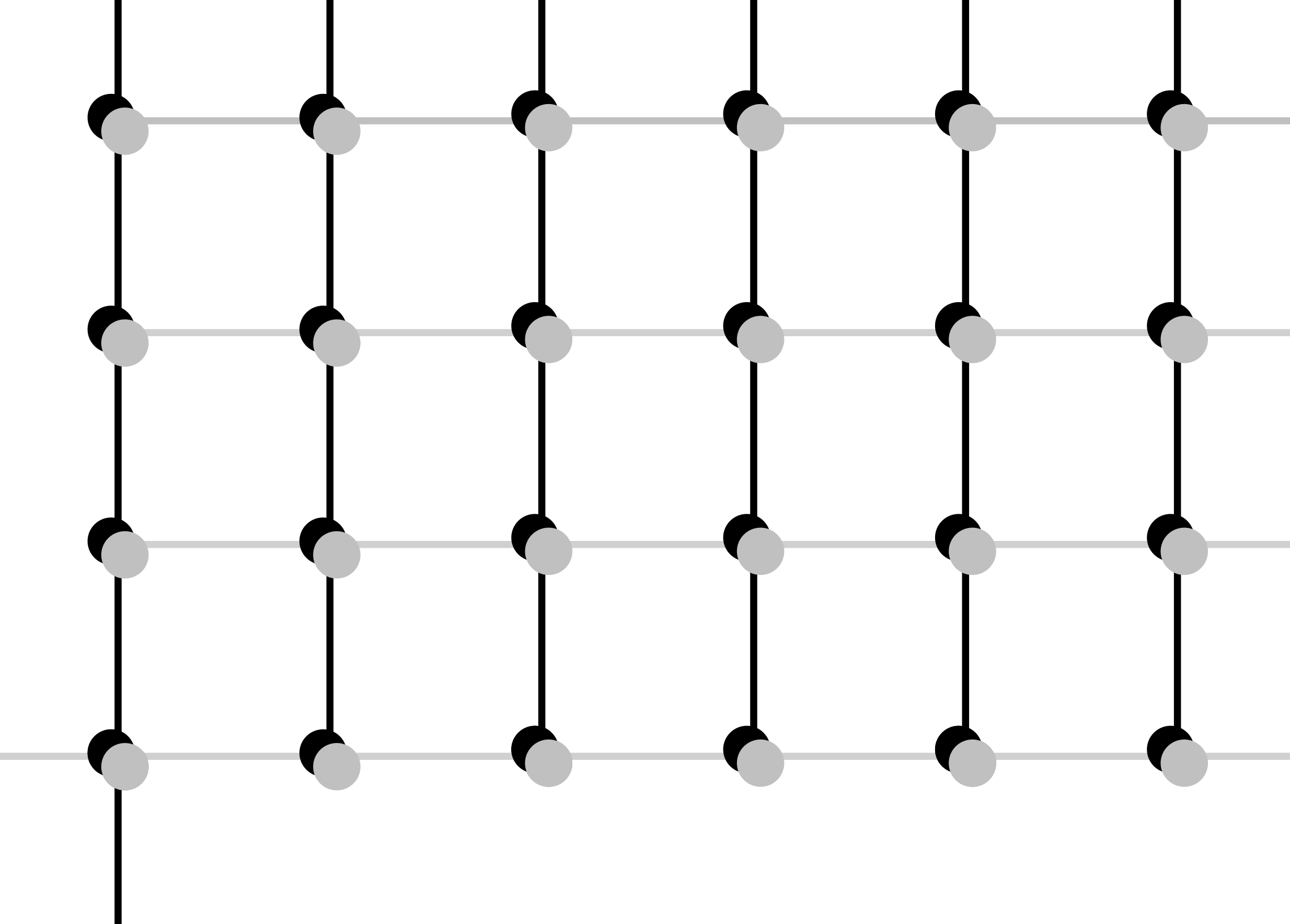
Figure 2: Illustration of $\mathbb{Z}_{+}^{2}\times H$. Points of form $(\cdot,\cdot,A)$ are represented by gray dots while $(\cdot,\cdot,B)$ points are represented by black dots. The extension to grid lines is also shown, with gray and black lines corresponding to points having $A$ and $B$ last coordinate, respectively.

We are interested at the track at some $L=\rho n^{3/2}+O(n)\in\mathbb{Z}$ distance on the graph. This is represented by $\approx\rho n^{1/2}$ distance in the current grid where each segment represents an arc of the cycle. Formally, we need the slanted line of the following intersection points, see also Figure 3.

$$R=\{(x,y,h)\in\mathbb{R}_{+}^{2}\times H~{}|~{}(x\in\mathbb{Z}_{+},h=B)\textrm{ or }(y\in\mathbb{Z}_{+},h=A),kx+(n-k)y=L\},$$ (3)

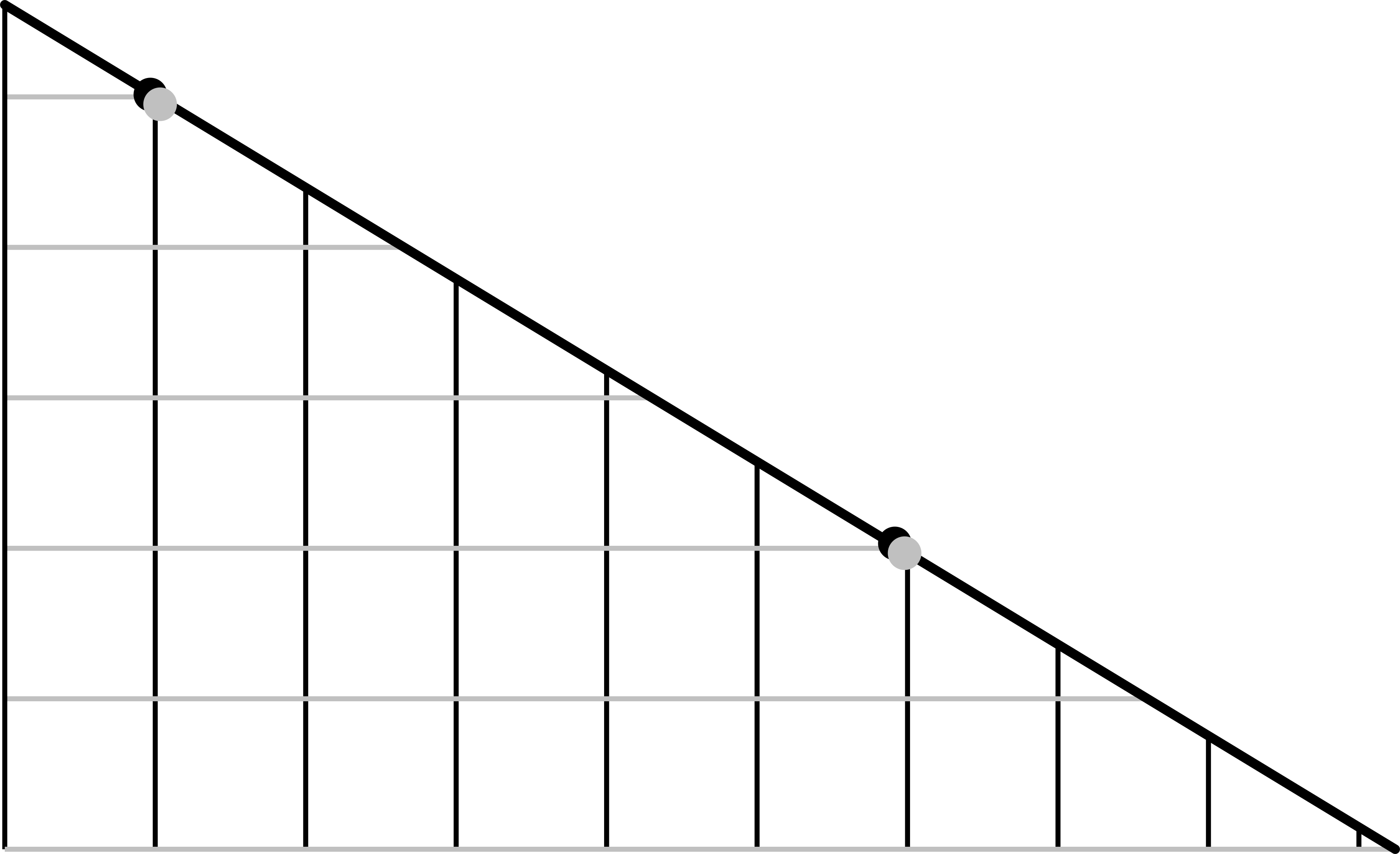
Figure 3: Illustration of $R$. An intersection of the slanted line with a grid line represents a single point in $R$ while passing through a grid point corresponds to two points in $R$.

Note that the constraints on the coordinates of the points of $R$ are sufficient so that they do properly map to vertices of the graph. Let us denote by $g:R\rightarrow V$ this function that recovers the vertex of the graph given a point in $R$. For $r\in R$ let us denote by $E_{r}$ the event that the Markov chain reaches $r$. Observe that these present a mutually exclusive partitioning of the probability space (except a null-set where the movement of the Markov-chain is bounded).

3.1 Exact expression for $E_{r}$ probabilities

The main goal of this section is to get usable bounds for $\mathbb{P}(E_{r})$. Let us examine how the Markov chain may reach $r$. The transition probabilities at the hubs imply that after traversing a horizontal unit segment there is $3/4$ probability to choose a vertical one and $1/4$ to take another horizontal one, and vice versa (and no backtracking can happen). For a fixed $r=(x,y,h)$ let us define the preceding grid point on $\mathbb{Z}_{+}^{2}$ in the $h$ direction $r^{\prime}=(x^{\prime},y^{\prime})$:

$$r^{\prime}=(x^{\prime},y^{\prime})=\begin{cases}\lceil x\rceil-1,y&\text{ if }h=A,\\ x,\lceil y\rceil-1&\text{ if }h=B.\end{cases}$$

We will simply use $x^{\prime},y^{\prime}$ by themselves if $r$ is clear from the context.

Lemma 4.

For $r\in R$ we have the following probability bound for reaching it:

$$\mathbb{P}(E_{r})\geq\frac{1}{4}\left[Binom(x^{\prime},3/4)*Binom(y^{\prime},1/4)\right](y^{\prime})\geq\frac{1}{9}\mathbb{P}(E_{r}),$$ (4)

where the $Binom$ stand for Binomial distributions and $*$ indicate their convolution.

Proof.

For the moment, let us assume that $r_{H}=B$, $X(0)_{H}=A$, and $x^{\prime},y^{\prime}>0$. The calculations for all other cases work similarly, we are going to discuss the differences afterwards.

We need to gather all possible routes to $r$ together with their probabilities. Assume that there were $2i+1$ changes of direction (it is certainly odd as a horizontal start ended on a vertical segment). This already determines that the probability of such a path is

$$\left(\frac{3}{4}\right)^{2i+1}\left(\frac{1}{4}\right)^{x^{\prime}+y^{\prime}-2i}.$$

To achieve $2i+1$ changes of directions, we need to split the total $x^{\prime}$ horizontal steps into $i+1$ parts, noting that a change may be valid after 0 steps due to the horizontal initialization. Consequently there are $x^{\prime}\choose i$ ways to do this. Similarly, there are $y^{\prime}\choose i$ possibilities to arrange the vertical steps. Altogether, we get

$$\mathbb{P}(E_{r})=\sum_{i=0}^{\infty}{x^{\prime}\choose i}{y^{\prime}\choose i}\left(\frac{3}{4}\right)^{2i+1}\left(\frac{1}{4}\right)^{x^{\prime}+y^{\prime}-2i}.$$

(The summation to $\infty$ is just for notational convenience, clearly there are only finitely many non-zero terms.) We may reformulate this as follows:

$$\mathbb{P}(E_{r}) =\sum_{i=0}^{\infty}{x^{\prime}\choose i}\left(\frac{3}{4}\right)^{i+1}\left(\frac{1}{4}\right)^{x^{\prime}-i}{y^{\prime}\choose y^{\prime}-i}\left(\frac{1}{4}\right)^{y^{\prime}-i}\left(\frac{3}{4}\right)^{i}$$ (5)

$$=\frac{3}{4}\left[Binom(x^{\prime},3/4)*Binom(y^{\prime},1/4)\right](y^{\prime}).$$

For all the scenarios in terms of the orientation of the first and last segment, we can perform the same computation. Collecting all the similar expressions together we get:

$$X(0)_{H}=A,r_{H}=B\quad\Rightarrow\quad\mathbb{P}(E_{r}) =\frac{3}{4}\left[Binom(x^{\prime},3/4)*Binom(y^{\prime},1/4)\right](y^{\prime}).$$ (6)

$$X(0)_{H}=A,r_{H}=A\quad\Rightarrow\quad\mathbb{P}(E_{r}) =\frac{3}{4}\left[Binom(x^{\prime}+1,3/4)*Binom(y^{\prime}-1,1/4)\right](y^{\prime}),$$ (7)

$$X(0)_{H}=B,r_{H}=B\quad\Rightarrow\quad\mathbb{P}(E_{r}) =\frac{3}{4}\left[Binom(x^{\prime}-1,3/4)*Binom(y^{\prime}+1,1/4)\right](y^{\prime}),$$ (8)

$$X(0)_{H}=B,r_{H}=A\quad\Rightarrow\quad\mathbb{P}(E_{r}) =\frac{3}{4}\left[Binom(x^{\prime},3/4)*Binom(y^{\prime},1/4)\right](y^{\prime}).$$ (9)

For our further work it will be convenient to avoid case splitting. Observe that each distribution is a sum of $x^{\prime}+y^{\prime}$ bits with very minor difference. This means that, for instance comparing (6) and (7), we have for any $s\in[0,1,\ldots,x^{\prime}+y^{\prime}]$

$$\frac{1}{3}\leq\frac{\left[Binom(x^{\prime}+1,3/4)*Binom(y^{\prime}-1,1/4)\right](s)}{\left[Binom(x^{\prime},3/4)*Binom(y^{\prime},1/4)\right](s)}\leq 3,$$

as the two distributions can be perfectly coupled except for a single bit of probability $3/4$ being coupled to a bit of probability $1/4$. Using the same comparison for the other cases with the reference (6) and accepting this error margin we get the overall bounds

$$\mathbb{P}(E_{r}) \geq\frac{1}{4}\left[Binom(x^{\prime},3/4)*Binom(y^{\prime},1/4)\right](y^{\prime}),$$

$$\frac{1}{3}\mathbb{P}(E_{r}) \leq\frac{3}{4}\left[Binom(x^{\prime},3/4)*Binom(y^{\prime},1/4)\right](y^{\prime}),$$

which combine together to give the statement of the lemma. This is now valid irrespective of directions. Even more, this final inequality holds true when $x^{\prime}=0$ or $y^{\prime}=0$ (although we will not need it). ∎

In the next subsection we aim to bound this in a simpler form. We want to emphasize that using the two Binomial distributions and evaluating their convolution at one point provides the probability for a single $E_{r}$, different distributions are needed for other elements of $R$.

3.2 Simplified estimates of $E_{r}$ probabilities

We will give estimates for points which are close to the diagonal. Define

$$R_{0}=\{r\in R~{}|~{}|x^{\prime}-y^{\prime}|\leq\sqrt{\rho}n^{1/4}\}.$$

By the definition (3) of $R$ we get

$$\min(x^{\prime},y^{\prime})n\leq L\leq\max(x^{\prime},y^{\prime})n,$$

which ensures $x^{\prime},y^{\prime}\in\left[\rho n^{1/2}-\sqrt{\rho}n^{1/4}+O(1),\rho n^{1/2}+\sqrt{\rho}n^{1/4}+O(1)\right]$ within this set.

Lemma 5.

There exists constant $\gamma_{1}>0$ such that for $n$ large enough and any point $r\in R_{0}$ we have

$$\mathbb{P}(E_{r})\geq\frac{\gamma_{1}}{\sqrt{\rho}n^{1/4}}.$$ (10)

Clearly this is what one would expect from CLT asymptotics, and such bounds are widely available for simple Binomial distributions. Here is one possible way to confirm the claim for our non-homogeneous case.

Proof.

Let

$$Q=Binom(x^{\prime},3/4)*Binom(y^{\prime},1/4),$$

the distribution appearing in (5). It can be viewed as the sum of $x^{\prime}+y^{\prime}$ independent indicators. We will approximate $Q$ with a Gaussian variable in a quantitative way using the Berry-Esseen theorem.

For an indicator with probability $1/4$ the variance is $3/16$, the absolute third moment after centralizing is $15/128$, we get the same values for the indicator with probability $3/4$ due to symmetry. Consequently we may consider the approximation

$$Q\approx\mathcal{N}\left(\frac{3x^{\prime}+y^{\prime}}{4},\frac{3x^{\prime}+3y^{\prime}}{16}\right).$$

Denoting by $F_{Q}$ and $F_{\mathcal{N}}$ the cumulative distribution functions of $Q$ and the properly scaled Gaussian above, the Berry-Esseen theorem (for not identically distributed variables) ensures

$$\sup_{\xi\in\mathbb{R}}|F_{Q}(\xi)-F_{\mathcal{N}}(\xi)|\leq\beta_{1}\left(\frac{3}{16}(x^{\prime}+y^{\prime})\right)^{-3/2}\frac{15}{128}(x^{\prime}+y^{\prime})=\frac{\beta_{2}}{(x^{\prime}+y^{\prime})^{1/2}},$$ (11)

where $\beta_{1}>0$ is the global constant of the theorem. Combining with the necessary second and third moments of our sum of independent variables added up, we get an explicit constant $\beta_{2}>0$ for the current problem. Note that the Berry-Essen theorem is originally stated for centered and normalized sums, but joint shifting and scaling does not change the difference of the cumulative distribution functions.

Let us now introduce the normalized distribution $\tilde{Q}$ by

$$\tilde{Q}\left(\left(C-\frac{3x^{\prime}+y^{\prime}}{4}\right)\frac{4}{\sqrt{3x^{\prime}+3y^{\prime}}}\right)=Q(C)$$

for any measurable set $C$, which is then approximated by the standard Gaussian distribution $\Phi$ (but is still a discrete distribution). This definition implies that in (5) we need the value of

$$\beta_{3}=\tilde{Q}\left(\left\{\alpha\right\}\right),\quad\text{where }\alpha=\frac{\sqrt{3}(y^{\prime}-x^{\prime})}{\sqrt{x^{\prime}+y^{\prime}}}.$$

Observe that by the definition of $R_{0}$ we have $|\alpha|<\sqrt{3/2}+O(n^{-1/8})<3/2$, for $n$ large enough. Define the intervals

$$I_{-}=\left[-2,-\frac{3}{2}\right],\quad I_{+}=\left[\frac{3}{2},2\right].$$

Recall that Binomial distributions are log-concave, so is their convolution $Q$, and its affine modification $\tilde{Q}$. Consequently, for any grid point the probability is at least all those that precede it or at least all those that are after it. In particular, $\beta_{3}$ is bounded below by all the (grid point) probabilities of $I_{-}$ or $I_{+}$. Simplifying further, we can take the average probabilities on the intervals, the lower will be a valid lower bound for $\beta_{3}$.

By the Berry-Essen estimate (11) we have that

$$q_{-}=\tilde{Q}(I_{-}) =\Phi\left(\left[-2,-\frac{3}{2}\right]\right)+O(n^{-1/4}),$$

$$q_{+}=\tilde{Q}(I_{+}) =\Phi\left(\left[\frac{3}{2},2\right]\right)+O(n^{-1/4}).$$

To estimate the number of grid points in the two intervals, we refer back to the unnormalized distribution $Q$ where we have to count the integers in the corresponding intervals, considering the scaling used. As an upper bound $m$ for the number of contained grid points we get

$$m\leq\left\lfloor\frac{1}{2}\frac{\sqrt{3x^{\prime}+3y^{\prime}}}{4}\right\rfloor+1\leq\frac{\sqrt{6\rho}}{8}(n^{1/4}+O(n^{1/8}))+1\leq\frac{1}{2}\sqrt{\rho}n^{1/4}+O(n^{1/8}).$$

Combining our observations and estimates we get to bound by the averages as

$$\beta_{3}\geq\frac{\min(q_{-},q_{+})}{m}\geq\frac{\Phi([3/2,2])+O(n^{-1/4})}{(1/2)\sqrt{\rho}n^{1/4}+O(n^{1/8})}=\frac{\beta_{4}}{\sqrt{\rho}n^{1/4}}+O(n^{-1/8}).$$

Finally, plugging this bound on $\beta_{3}$ into (4) we arrive at

$$\mathbb{P}(E_{r})\geq\frac{\gamma_{1}}{\sqrt{\rho}n^{1/4}},$$

for any $0<\gamma_{1}<\beta_{4}/4$ and $n$ large enough, which matches the claim of the lemma.

∎

4 Mapping the grid to the cycle

In the previous section using the grid we have abstractly identified points $R$ at appropriate distance from the starting position and also points $R_{0}\subseteq R$ which are reached with non-negligible probabilities. As the next step, we want to understand what these points represent on the original cycle. W.l.g. we assume $k\leq n/2$.

Lemma 6.

We have $\sqrt{\rho}n^{1/4}+O(1)\leq|R_{0}|\leq 4\sqrt{\rho}n^{1/4}+O(1)$.

Proof.

For the moment, let us use the notation $\tilde{L}=L/n=\rho n^{1/2}+O(1)$. Using this for both $x$ and $y$ would solve the defining equation $kx+(n-k)y=L$. Thus for any integer $x\in[\tilde{L}-\frac{1}{2}\sqrt{\rho}n^{1/4}+1,\tilde{L}+\frac{1}{2}\sqrt{\rho}n^{1/4}-1]$ there is a corresponding $y$ in the same interval that solves the defining equation. Here we use the assumption $k\leq n-k$, so that $y$ will differ no more from the center value than $x$. Therefore $|x-y|\leq\sqrt{\rho}n^{1/4}-2$ which is enough to ensure the pair accompanied by a $B$ being in $R_{0}$. The number of integers in the given interval confirms the lower bound.

Adjusting the above argument, check the approximately double width interval $x\in[\tilde{L}-\sqrt{\rho}n^{1/4},\tilde{L}+\sqrt{\rho}n^{1/4}],x\in\mathbb{Z}$, which is a necessary condition for being in $R_{0}$ and of form $(\cdot,\cdot,B)$. There will be at most one such point in $R_{0}$ for each $x$, so $2\sqrt{\rho}n^{1/4}+O(1)$ in total. Now counting the points on horizontal grid lines (collecting $(\cdot,\cdot,A)$ points), for any $y\in[\tilde{L}-\sqrt{\rho}n^{1/4},\tilde{L}+\sqrt{\rho}n^{1/4}],y\in\mathbb{Z}$ there will be at most one matching $x\in\mathbb{R}$ again. Adding up the two cases we get the upper bound. ∎

It will be easier to handle a set of points of known size, so let $R_{1}\subseteq R_{0}$ be a subset of size $\sqrt{\rho}n^{1/4}$ (or maybe $O(1)$ less) of the elements in the middle.

We want to convert our grid representation to the cycle and acquire the image of $R_{1}$, that is,

$$V_{1}=\{g(r)~{}|~{}r\in R_{1}\}.$$

To understand this set we scan through the elements of $R_{1}$, starting with the one with the lowest $x$ and increasing (taking direction $A$ before $B$ when passing through a grid point) and follow where do they map on the cycle. When moving from one point, $U$, to the next, $U^{\prime}$, we may encounter the following configurations, as shown in Figure 4:

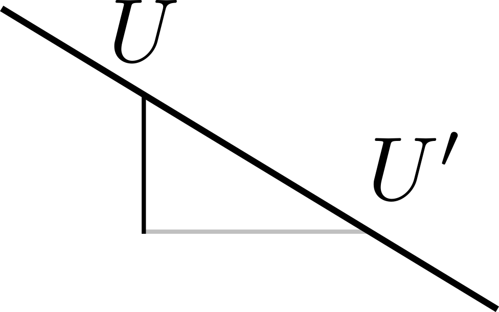
(i)

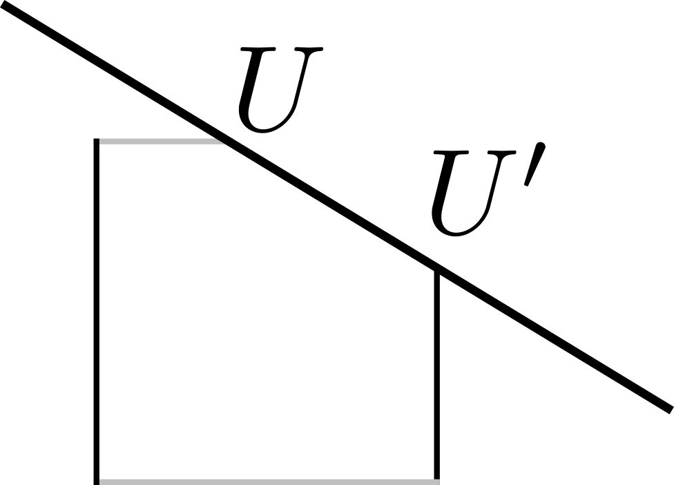
(ii)

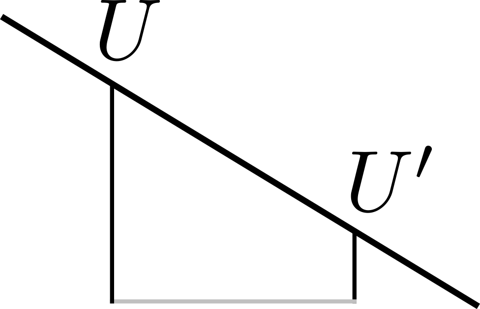
(iii)

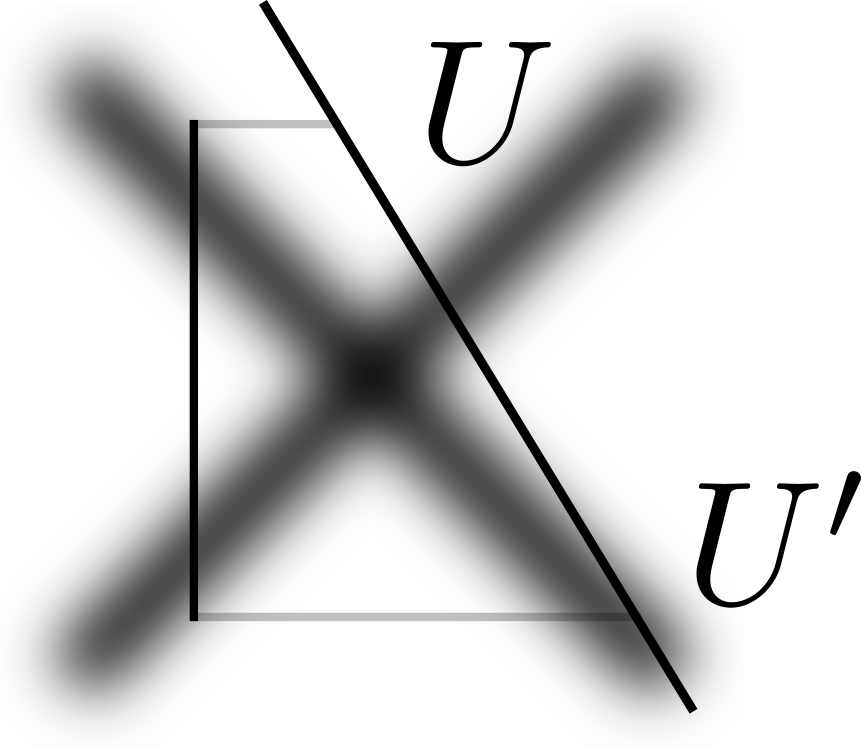
(iv)

Figure 4: Possible transitions depicted as $U\rightarrow U^{\prime}$ while scanning through $R_{1}$.

• In case (i) we see that the final few $l$ steps (out of $L$) are starting on the $B$ arc for $U$ and starting on the $A$ arc for $U^{\prime}$. Consequently, $U^{\prime}$ can be reached from $U$ by exactly $k$ counter-clockwise steps on the cycle.

• In case (ii) we almost reach the next grid point, some $l$ steps are missing on the $A$ arc for $U$ and also $l$ steps are missing on the $B$ arc for $U^{\prime}$. This means, again, that $U^{\prime}$ can be reached from $U$ by exactly $k$ counter-clockwise steps on the cycle.

• In case (iii) we are on the $B$ arc for both $U$ and $U^{\prime}$ but we had one more horizontal $A$ segment for $U^{\prime}$ (representing $k$ steps) which is missing from the height. Therefore we get the same, $U^{\prime}$ can be reached from $U$ by exactly $k$ counter-clockwise steps on the cycle.

• Passing through a grid point can be treated as the special case of either (i) or (ii), with the same consequence. Note that case (iv) can not happen due to our assumption of $k\leq n/2$.

To sum up, we can generate the set $V_{1}\subset V$ on the cycle corresponding to $R_{1}$ by finding the first vertex, then taking jumps of $-k$ (modulo $n$) for $|R_{1}|-1$ more steps. We want to ensure the elements of $V_{1}$ are spread out enough.

Lemma 7.

There exist constants $\gamma_{2}>0$ and $\gamma_{3}>\frac{1}{2}$ such that the following holds for large enough $n$. For a uniform choice of $k\in[2,3,\ldots,n-2]$ with probability at least $\gamma_{2}$ we have

$$\forall v,v^{\prime}\in V_{1},~{}v\neq v^{\prime}:~{}|v-v^{\prime}|\geq\frac{\gamma_{3}}{\sqrt{\rho}}n^{3/4}.$$ (12)

Proof.

We will use $\gamma_{3}$ as a parameter for now which we will specify later. We will consider a uniform choice $k\in[1,2,\ldots,n]$ for convenient calculations, clearly this does not change the probability asymptotically.

Two elements of $V_{1}$ get close if after some repetitions of the $k$-jumps, we get very close to the start (after a few full turns). More precisely the condition is violated iff

$$\exists 1\leq m\leq|R_{1}|-1\quad|mk|<\frac{\gamma_{3}}{\sqrt{\rho}}n^{3/4}.$$

Our goal is to have a $k$ so that this not happen. For a fixed $m$ this excludes $k$ from the intervals

$$\left(\frac{in-\frac{\gamma_{3}}{\sqrt{\rho}}n^{3/4}}{m},\frac{in+\frac{\gamma_{3}}{\sqrt{\rho}}n^{3/4}}{m}\right),\quad i=0,1,\ldots,m-1.$$

To simplify our calculations we will treat these intervals as real intervals on the cycle (rather than an interval of integers). Length and number of integers contained differ by at most one, we will correct for this error at the end.

We need to merge these intervals for all $1\leq m\leq|R_{1}|-1$. We imagine doing this by collecting the intervals as increasing $m$. Observe that if $\gcd(i,m)=c>1$, then we already covered the interval around $\frac{in}{m}$ when encountering $\frac{(i/c)n}{m/c}$, and by a wider interval. That is, we only have to count those $i$ where $\gcd(i,m)=1$. Therefore the total newly covered area at step $m$ is at most

$$\frac{2\gamma_{3}}{\sqrt{\rho}}n^{3/4}\frac{\varphi(m)}{m},$$

where $\varphi$ denotes the classical Euler function. Once we add these up, and use the summation approximation [8] we get

$$\frac{2\gamma_{3}}{\sqrt{\rho}}n^{3/4}\sum_{m=1}^{|R_{1}|-1}\frac{\varphi(m)}{m}=2\gamma_{3}\frac{6}{\pi^{2}}n+O(n^{3/4}\log n),$$ (13)

knowing that $|R_{1}|=\sqrt{\rho}n^{1/4}+O(1)$. When we switched from integer counts to approximation by interval lengths, the total error is at most 1 per interval, that is,

$$\sum_{m=1}^{|R_{1}|-1}m=O(n^{1/2}),$$

which is negligible compared to the quantities of (13). Consequently (13) is an upper bound on the number of $k$ that should be excluded. Let us therefore choose $\gamma_{3}>1/2$ so that the coefficient of $n$ above is strictly less than 1. Then there is still strictly positive probability to pick a good $k$, in particular

$$\gamma_{2}=1-\frac{12\gamma_{3}}{\pi^{2}}-\varepsilon$$

is adequate for any small $\varepsilon>0$. ∎

5 Including diffusive behavior

So far we have understood the position of the chain after $L$ moves from the first grid point. Now we want to analyze the true Markov chain dynamics where moving or staying in place is also random. In $V_{1}$ we have a large number of positions, hopefully different and separated enough, and we can bound the probability of reaching the corresponding elements in $R_{1}$.

For technical reasons to follow, we want to avoid points in $V_{1}$ that are very close to the hubs so define

$$V_{2} =\{v\in V_{1}~{}|~{}|v-k|,|v-n|>4\sqrt{\rho}n^{3/4}\sqrt{\log n}\},$$

$$W =\{w\in V~{}|~{}\exists v\in V_{2},~{}|w-v|<\gamma_{3}\sqrt{\rho}n^{3/4}/2\},$$ (14)

$$R_{2} =\{r\in R_{1}~{}|~{}g(r)\in V_{2}\}.$$

We would like to emphasize that in the favorable case when (12) holds (ensured with positive probability by Lemma 7), we have $|V_{2}|,|R_{2}|=\sqrt{\rho}n^{1/4}+O(\sqrt{\log n})$ and when $\rho\leq 1$ this also implies $|W|=\gamma_{3}\rho n+O(n^{3/4}\sqrt{\log n})$.

At most vertices, a $Geo(1/2)$ distribution controls when to step ahead, so let us choose some

$$T=2\rho n^{3/2}+O(n)\in 2\mathbb{Z}$$

and analyze $X(T)$. Oversimplifying the situation at first, in $T$ steps the chain travels $T/2$ in expectation, $O(n)$ to reach the origin grid point, $\rho n^{3/2}+O(n)$ afterwards, which is exactly the case analyzed. We have control of the probability of $\approx\sqrt{\rho}n^{1/4}$ of the expected endpoints, and we will have a diffusion $\approx\sqrt{\rho}n^{3/4}$ around them, which together will provide a nicely spread out distribution.

However, there are some non-trivial details hidden here. The most important caveat is that when visiting the hubs, the distribution of the time spent is not independent of the direction taken. In fact, when arriving at a hub, say at vertex $a_{k}$, with probability $1/2$ there is a single step, going to $b_{1}$. Otherwise, some loops, jumps are taken between the hubs before moving on, which tells that with probability $1/4,1/4$ the chain continues to $a_{1},b_{1}$, in $1+Geo(1/2)$ steps. Let us combine all the heuristics and work out the details in a formally precise way.

We are going to describe a procedure to generate the Markov chain and the position $X(T)$. If $X(0)$ is $\lambda$ steps before one of the hubs, thus the origin grid point, fix $L=T/2-\lambda=\rho n^{3/2}+O(n)$, define $R$ with this value in (3). Assume we are given an infinite i.i.d. series of fair coin tosses which may either tell go ($1$) or do nothing ($0$). We perform the following steps.

• Choose the exit point $r\in R$, with appropriate probability $\mathbb{P}(E_{r})$.

• Choose one of the possible tracks $\xi$ reaching $r$ (with the appropriate conditional probability).

• Generate a series of coin tosses $c_{0}$ of length $T-(x^{\prime}+y^{\prime}+1)$, which is the major part of the movement of the chain.

• Complement the above series depending on the track. Following the Markov chain using the beginning of $c_{0}$, when we reach a hub where the direction should be continued according to $\xi$ ($AA$ or $BB$), insert an extra $0$ symbol (correcting for the $1+Geo(1/2)$ waiting time distribution there). Similarly, when we reach a hub where the direction changes ($AB$ or $BA$), with probability $2/3$ insert a $1$ (meaning an instant step), with probability $1/3$ insert a $0$ (for the $1+Geo(1/2)$ case). If we encounter a grid point further than $r$, we freely choose the direction together with the inserted symbol with probabilities $1/4,1/2,1/4$ for the 3 cases we had. Let the elongated series be $c_{1}$, the sequence of only the added symbols be $c_{h}$.

Let us use the notation $|c_{0}|$ for the length of $c_{0}$ and $\sum(c_{0})$ for the number of $1$-s in $c_{0}$ (and similarly for the other sequences). Let us also introduce $\tau=|c_{1}|$. Therefore at the end of the procedure above we arrive at $X(\tau)$. More importantly, $\tau$ matches $T$ very well as stated below.

Lemma 8.

For $r\in R_{2}$ we have

$$\mathbb{P}(\tau=T)=1-O(n^{-4}).$$

Proof.

In $c_{0}$ for the number of $1$ symbols we have

$$\left|\sum(c_{0})-(L+\lambda)\right|\leq\left|\sum(c_{0})-\frac{1}{2}(T-(x^{\prime}+y^{\prime}+1))\right|+\left|\frac{1}{2}(T-(x^{\prime}+y^{\prime}+1))-(L+\lambda)\right|.$$

The second term on the right hand side is $O(n^{1/2})$ by the definitions. For the term before we can use standard tail probability estimates for the Binomial distribution (based on Hoeffding’s inequality). Merging the two error terms we get

$$\mathbb{P}\left(\left|\sum(c_{0})-(L+\lambda)\right|>3\sqrt{\rho}n^{3/4}\sqrt{\log n}\right)=O(n^{-4}).$$ (15)

Let us denote this bad event of the left side above by $\mathcal{B}$ for future use. Assume that this event does not occur, and $\sum(c_{0})$ is within the error bound $3\sqrt{\rho}n^{3/4}\sqrt{\log n}$. This means that the Markov chain takes the first $\lambda$ steps to the origin and then $\approx L$ steps within the stated bounds.

By the definition of $R_{2}$ this concentration tells that even only considering the $c_{0}$ steps we reach the grid line segment where $r$ lies. On the way we pass through $x^{\prime}+y^{\prime}+1$ hubs, which results in $x^{\prime}+y^{\prime}+1=O(n^{1/2})$ entries in $c_{h}$. Conversely, inserting this $O(n^{1/2})$ steps into $c_{0}$ the upper bound ensures that we will not reach the next grid point (or the hub once more, in other words). Consequently, $|c_{h}|=x^{\prime}+y^{\prime}+1$.

Therefore in this case we have $\tau=|c_{1}|=|c_{0}|+|c_{h}|=T$, which we wanted to show, the exceptional probability is controlled by (15) which matches the claim. ∎

Lemma 9.

For any $w\in W$ we have

$$\mathbb{P}(X(T)=w)\geq\frac{\gamma_{4}}{\rho n},$$

for an appropriate global constant $\gamma_{4}>0$.

Proof.

By the definition of $W$ there is a $v=g(r)\in V_{2}$ with $|v-w|\leq\frac{\gamma_{3}\sqrt{\rho}}{2}n^{3/4}$ (if multiple, we choose one). We use the procedure above to actually bound the probability for $X(\tau)$, but by Lemma 8 we know this is correct up to $O(n^{-4})$ error which is enough for our case. In the process let us consider the case where $E_{r}$ is chosen and also some track $\xi$ is fixed.

With these conditions, let us analyze the dependence structure of the step sequences. For $c_{1}$, the positions of the additions strongly depend on $c_{0}$. However, we know exactly what hubs and which turns we are going to take, which means $c_{h}$ is independent of $c_{0}$ (assuming $\bar{\mathcal{B}}$), only their interlacing depends on both.

Now, first drawing and fixing $c_{h}$ we know by $\sum(c_{h})$ precisely how many $1$-s do we need from $c_{0}$ to exactly hit $w$ (still conditioning on $E_{r}$ and $\xi$). Let this number be $s$, for which we clearly have $|s-\rho n^{3/2}|\leq\gamma_{3}\sqrt{\rho}n^{3/4}/2+O(n^{1/2})$. The length of $c_{0}$ is $T^{\prime}=T-(x^{\prime}+y^{\prime}+1)=T+O(\sqrt{n})$. We have to approximate this Binomial probability of $1$-s in $c_{0}$. This is a tedious calculation based on the Stirling formula, we refer to [7] where it is shown that

$${T^{\prime}\choose s}=(1+o(1))\frac{2^{T^{\prime}}}{\sqrt{T^{\prime}\pi/2}}\exp\left(-\frac{(T^{\prime}-2s)^{2}}{2T^{\prime}}\right),$$

if $|T^{\prime}/2-s|=o(T^{\prime 2/3})$ which clearly holds in our case. Substituting the variables we get the bound

$${T^{\prime}\choose s}\frac{1}{2^{T^{\prime}}}\geq(1+o(1))\frac{1}{\sqrt{\pi\rho}n^{3/4}}\exp\left(-\frac{\gamma_{3}^{2}}{4}+O(n^{-1/4})\right)\geq\frac{\beta_{1}}{\sqrt{\rho}n^{3/4}},$$

for some constant $\beta_{1}>0$ and $n$ large enough. Thus, for the conditional probability of interest we get

$$\mathbb{P}(X(T)=w~{}|~{}E_{r},\xi,c_{h})\geq\frac{\beta_{1}}{\sqrt{\rho}n^{3/4}}-\mathbb{P}(\mathcal{B})\geq\frac{\beta_{2}}{\sqrt{\rho}n^{3/4}}$$

for any constant $\beta_{1}>\beta_{2}>0$ and $n$ large enough.

Observe that we have the same lower bound for $\mathbb{P}(X(T)=w~{}|~{}E_{r})$ as it is a mixture of the conditional probabilities above, so we can average out through $\xi$ and $c_{h}$. Finally, combining with (10) we arrive at

$$\mathbb{P}(X(T)=w)\geq\mathbb{P}(X(T)=w~{}|~{}E_{r})\mathbb{P}(E_{r})\geq\frac{\gamma_{4}}{\rho n},$$

with an appropriate constant $\gamma_{4}>0$. ∎

6 Global mixing

We now turn to evaluating the mixing metrics of our Markov chain. In order to establish the upper bound on the mixing time initially claimed in Theorem 2 we fix $\rho=1$ and $T=2\lceil\rho n^{3/2}\rceil$ for this section and use previous results using these parameters. We will drop $X$ from indices and arguments in (1), (2) when clear from the context.

An alternative of $d(t)$ compares the distribution of the Markov chain when launched from two different starting points:

$$\bar{d}(t):=\sup_{X^{1}(0),X^{2}(0)\in V}\|\mathcal{L}(X^{1}(t))-\mathcal{L}(X^{2}(t))\|_{\rm TV}.$$

It is known how this compares with $d(t)$, we have the inequalities $d(t)\leq\bar{d}(t)\leq 2d(t)$, moreover this variant is submultiplicative, $\bar{d}(s+t)\leq\bar{d}(s)\bar{d}(t)$, see [6, Chapter 4]. We can quantify this distance for our problem as follows.

Lemma 10.

Assume that $n$ is large enough and $k$ is such that (12) holds. Then we have

$$\bar{d}(T)\leq 1-\gamma_{5},$$ (16)

for some global constant $\gamma_{5}>0$.

Proof.

Fix two arbitrary starting vertices for $X^{1}(0)$ and $X^{2}(0)$ and denote the distribution of the two chains at time $T$ by $\sigma^{1},\sigma^{2}$. Simple rearrangements yield

$$\|\sigma^{1}-\sigma^{2}\|_{\rm TV} =\frac{1}{2}\sum_{v\in V}|\sigma^{1}(v)-\sigma^{2}(v)|=\frac{1}{2}\sum_{v\in V}(\sigma^{1}(v)+\sigma^{2}(v)-2\min(\sigma^{1}(v),\sigma^{2}(v)))$$ (17)

$$=1-\sum_{v\in V}\min(\sigma^{1}(v),\sigma^{2}(v)).$$

For both realizations in (14) we get a subset of vertices, $W^{1},W^{2}$, and there must be a considerable overlap, in particular

$$|W^{1}\cap W^{2}|\geq|W^{1}|+|W^{2}|-n=(2\gamma_{3}-1)n+O(n^{3/4}\sqrt{\log n})\geq\beta n$$

for some $\beta>0$ and $n$ large enough, relying on the fact that $\gamma_{3}>1/2$. By Lemma 9 for any $w\in W^{1}\cap W^{2}$ we have both $\sigma^{1}(w),\sigma^{2}(w)\geq\gamma_{4}/n$. Substituting this back to (17) we get

$$\|\sigma^{1}-\sigma^{2}\|_{\rm TV}\leq 1-\beta n\frac{\gamma_{4}}{n}=1-\gamma_{5},$$

with $\gamma_{5}=\beta\gamma_{4}$. This upper bound applies for any two starting vertices of $X^{1},X^{2}$, therefore the claim follows. ∎

We just need the final touch to prove Theorem 2.

Proof of Theorem 2.

Using Lemma 7 we have a spread out collection in $V_{2}$ as stated in (12) with probability at least $\gamma_{2}=:\gamma$. In this case we can apply Lemma 10. Fix

$$T^{*}=\left\lceil\frac{\log\varepsilon}{\log(1-\gamma_{5})}\right\rceil T.$$

Substituting (16) and using the basic properties of $d,\bar{d}$ we get

$$d(T^{*})\leq\bar{d}(T^{*})\leq\bar{d}(T)^{\left\lceil\frac{\log\varepsilon}{\log(1-\gamma_{5})}\right\rceil}\leq(1-\gamma_{5})^{\left\lceil\frac{\log\varepsilon}{\log(1-\gamma_{5})}\right\rceil}\leq\varepsilon.$$

Consequently, $t_{\rm mix}(\varepsilon)\leq T^{*}$. On the other hand,

$$T^{*}=\left\lceil\frac{\log\varepsilon}{\log(1-\gamma_{5})}\right\rceil T=\left\lceil\frac{\log\varepsilon}{\log(1-\gamma_{5})}\right\rceil 2\lceil n^{3/2}\rceil\leq\gamma^{\prime}n^{3/2}\log\frac{1}{\varepsilon},$$

for appropriate constant $\gamma^{\prime}>0$ and $n$ large enough. Together with the previous calculation this confirms the theorem. ∎

7 Lower bound

In this section let us fix $\rho=\gamma_{4}/2$. Lemma 9 tells that at elements of $W$ there is $2/n$ probability of the Markov chain to arrive, however, we have no information on the size of $W$ for general $k$, for all edge selections, and there might be significant overlaps, multiplicities when defining $V_{1}$ or $W$. It is key for completing the proof to be able to handle this.

We know $|R_{1}|=\sqrt{\rho}n^{1/4}+O(1)$ but we have no size estimates on $|R_{2}|,|V_{2}|$. Let the set of interest be

$$I=\{v\in V~{}|~{}|v-k|,|v-n|>4\sqrt{\rho}n^{3/4}\sqrt{\log n}\}.$$

For the moment we cannot guarantee that most of $R_{1}$ maps into $I$. In order to change this, we start moving time a bit. Let us define

$$T^{i} =2\lceil\rho n^{3/2}\rceil+2i,\qquad i=0,1,\ldots,n-1,$$

$$L^{i} =\lceil\rho n^{3/2}\rceil-\lambda+i,\qquad i=0,1,\ldots,n-1.$$

Accordingly, there is an evolution $R^{i}$ and $R_{0}^{i}$. Here $\lambda$ corresponds to the position of $X(0)$ as before, which is arbitrary, but we consider it as fixed.

For $R_{1}^{i}$ (together with $V_{1}^{i}$), we investigate this evolution from the perspective of the individual points. One can verify that a valid interpretation is that $r=(x,y,h)\in R_{1}^{0}$ performs a zigzag away from the origin along the grid lines stopping just before $(x+1,y+1,h)$, turning at both grid points it passes along the way. During the move $|x^{\prime}-y^{\prime}|$ changes by at most 1, so there can be edge effects whether the point is allowed in $R_{0}^{i}$ or not, but only at the very ends of $R_{1}^{i}$. This process is illustrated in Figure 5.

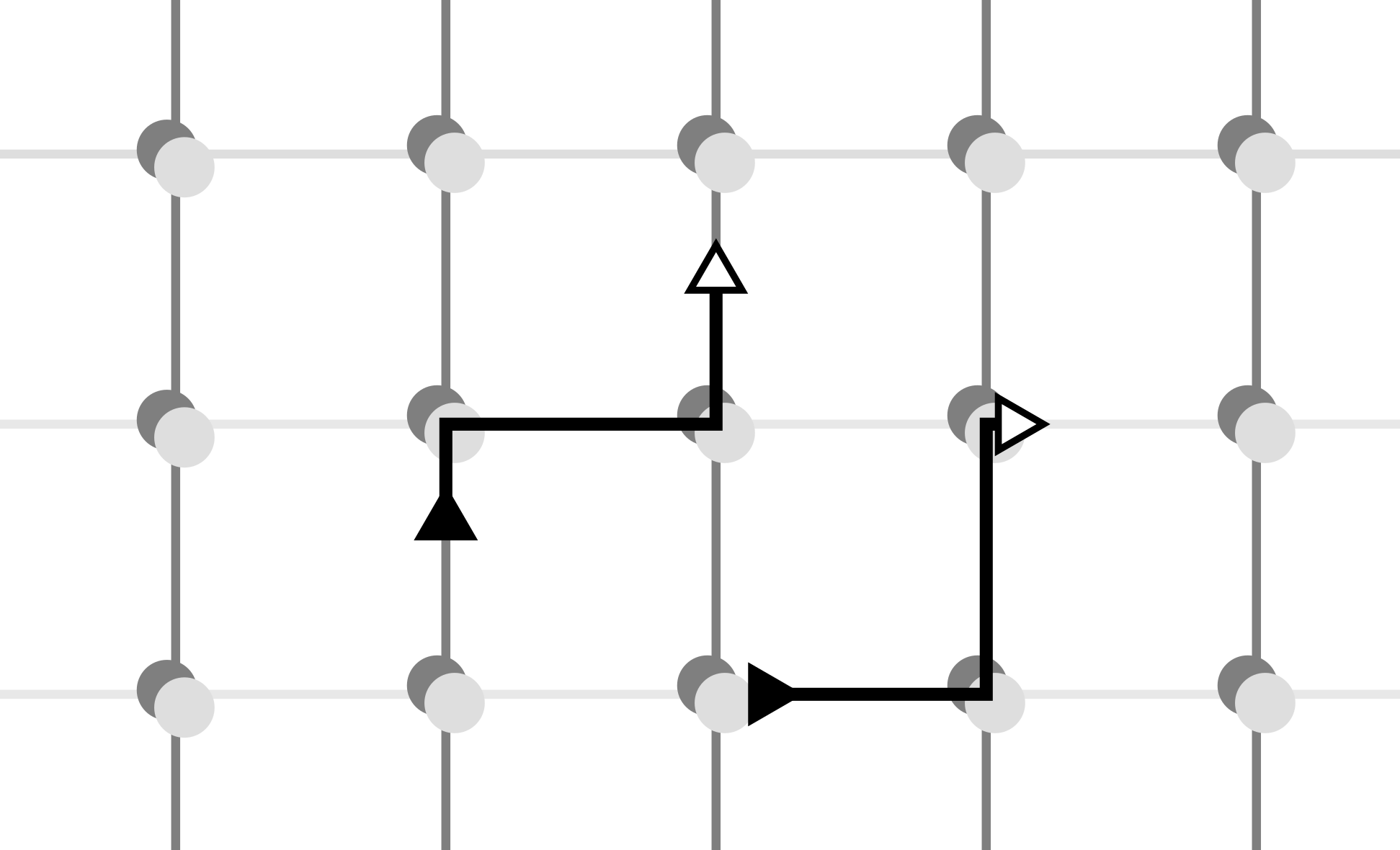
Figure 5: Evolution of the points of $R_{1}^{i}$ with the increase of $i$. Two such zigzag paths are depicted.

Observe that such a zigzag corresponds to walking around the cycle exactly once. This will allow us to conveniently calculate the total number of hits to $I$ by $V_{1}^{0},\ldots,V_{1}^{n-1}$. More precisely (to account for multiplicities), we are interested in

$$M=\sum_{i=0}^{n-1}\sum_{r\in R_{1}^{i}}\mathbbm{1}_{I}(g(r)).$$

By the previous argument we know that along each point the number of hits is exactly $I$, except maybe near the edges. Thus we get

$$M\geq|R_{1}|\cdot|I|-O(n).$$

Comparing the two while dividing by $n$ we get

$$\frac{1}{n}\sum_{i=0}^{n-1}\sum_{r\in R_{1}^{i}}\mathbbm{1}_{I}(g(r))\geq|R_{1}|\frac{|I|}{n}-O(1)\geq\frac{|R_{1}|}{2}.$$

Consequently, there has to be an index $i$ where the term on the left hand side being averaged out is larger than the right hand side:

$$\sum_{r\in R_{1}^{i}}\mathbbm{1}_{I}(g(r))\geq\frac{|R_{1}|}{2}.$$

Let us take and fix such an $i$ from now on. Define the analogous sets as before

$$R_{2}^{i} =\{r\in R_{1}^{i}~{}|~{}g(r)\in I\},$$

$$W^{i} =\{w\in V~{}|~{}\exists r\in R_{2}^{i},|g(r)-w|\leq\gamma_{3}\sqrt{\rho}n^{3/4}/2\}.$$

We now formulate an extension of Lemma 9:

Corollary 11.

For any $r\in R_{2}^{i}$, $w\in W^{i}$ such that $|g(r)-w|\leq\gamma_{3}\sqrt{\rho}n^{3/4}/2$ we have

$$\mathbb{P}(X(T^{i})=w,E_{r})\geq\frac{\gamma_{4}}{\rho n},$$

for the same global constant $\gamma_{4}>0$ as before.

Proof.

This is actually what is happening under the hood in the proof of Lemma 9, just there the choice of $r$ is given by the structure $W$ and the extra knowledge on $E_{r}$ is discarded at the end. ∎

Proof of Theorem 3.

We want to bound $d(T^{i})$, with the $i$ carefully chosen above. With only analyzing the case of the starting point fixed above we get a lower bound on $d(T^{i})$. We need to estimate the total variation distance:

$$\left\|\mathcal{L}(X(T^{i}))-\frac{\mathbbm{1}}{n}\right\|_{\rm TV}=\frac{1}{2}\sum_{v\in V}\left|P(X(T^{i})=v)-\frac{1}{n}\right|.$$

Note that for any $w\in W^{i}$ there is a corresponding $r$ nearby to apply Corollary 11, and with the choice of $\rho$ at the beginning of the section we get $P(X(T)=w)\geq 2/n$. That is, these terms in the sum are positive without the absolute value. We drop other values for a lower bound. Thus we get

$$\left\|\mathcal{L}(X(T^{i}))-\frac{\mathbbm{1}}{n}\right\|_{\rm TV}\geq\frac{1}{2}\sum_{w\in W^{i}}\left(P(X(T^{i})=w)-\frac{1}{n}\right)\geq\frac{1}{2}\sum_{r,w}\frac{2}{n}-\frac{1}{2}|W^{i}|\frac{1}{n}.$$

In the first term we may include all compatible pairs of $r,w$ for which Corollary 11 can be applied. Recall that $|R^{i}_{2}|\geq\sqrt{\rho}n^{1/4}/2+O(1)$, each element compatible with $\gamma_{3}\sqrt{\rho}n^{3/4}+O(1)$ number of $w$’s.

For the second term being subtracted, we may count very similarly starting from $R^{i}_{2}$ and looking for compatible pairs. This time however, multiplicity does not add up as we need the size of the set, but we want an upper bound for this term anyway. In total we get

$$\left\|\mathcal{L}(X(T^{i}))-\frac{\mathbbm{1}}{n}\right\|_{\rm TV}\geq\frac{1}{n}|R^{i}_{2}|\left({\gamma_{3}}{\sqrt{\rho}}n^{3/4}+O(1)\right)-\frac{1}{2n}|R^{i}_{2}|\left({\gamma_{3}}{\sqrt{\rho}}n^{3/4}+O(1)\right)\geq\frac{\gamma_{3}\rho}{4}+O(n^{-1/4}).$$

As $d(\cdot)$ is non-increasing, for the constants of the theorem we may choose $\gamma^{*}=2\rho=\gamma_{4}$ and any $\varepsilon^{*}<\gamma_{3}\rho/4=\gamma_{3}\gamma_{4}/8$. With such choices the previous calculations show that the claim holds.

∎

8 Discussion, conclusions

Let us further elaborate on the results obtained together with ideas for possible extensions.

First of all, Theorem 2 provides a global probability estimate for the mixing time bound to hold but is not an a.a.s. result. It is unclear if this is the result of our bounds being conservative, or because truly there is a large proportion of badly behaving $k$. Note that there are bad $k$, for instance if $n$ is even then for $k=n/2$ the mixing time is truly quadratic in $n$.

Concerning the proof technique, observe that the grid together with the grid lines correspond to a covering of the original graph which is well suited for our purpose.

An interesting question is whether there is an extension possible for slightly more connections. The more natural one is to increase the number of random edges. In this case however, one might need to handle the effects of the small permutations generated by the various edges. The more accessible one is to increase the number of random hubs, then adding all-to-all connections between them. Closely related work has been done for the asymptotic rate of convergence [5] when then number of hubs can grow at any small polynomial rate, and it turns out that in that case the inverse spectral gap is linear in the length of the arcs (excluding logarithmic factors), which would be a bottleneck anyway.

Still, we might guess the mixing time in a heuristic manner for constant number of hubs, with the generous assumption that our concepts can be carried over. Let us consider $K$ random hubs – and thus also $K$ arcs – and check mixing until $n^{\alpha}$ for some $\alpha$. We can assume the lengths of the arcs are of order $n$, so the set generalizing $R$ is on a $K-1$ dimensional hyperplane at distance $\approx n^{\alpha-1}$ from the origin. We can hope to get a CLT type control on the probability in a ball of radius $\approx n^{(\alpha-1)/2}$ again, thus the number of such points in the hyperplane is $\approx n^{(K-1)(\alpha-1)/2}$. If once again these map to far away points on the cycle and this movement can be nicely blended together with the diffusion, that would provide an extra factor of $\approx n^{\alpha/2}$, meaning the total number of vertices reached is

$$\approx n^{(K-1)\frac{\alpha-1}{2}+\frac{\alpha}{2}}=n^{\frac{K}{2}(\alpha-1)+\frac{1}{2}}.$$

We hope for mixing when the exponent reaches 1 which translates to $\alpha=1+1/K$, and leads us to the following conjecture:

Conjecture 12.

Consider $K\in\mathbb{Z}_{+},\varepsilon>0$ fixed. On a cycle of $n$ vertices, choose $K$ hubs randomly. With an appropriate interconnection structure among the hubs, and a Markov chain otherwise analogous to the one before there is a positive bounded probability to have

$$t_{\rm mix}(\varepsilon)=\Theta\left(n^{1+1/K}\right),$$

for $n$ large enough.

Clearly there is quite some flexibility left for the class of Markov chains to consider. This remains as a question for future research to find out exactly what is needed to generalize the current toolchain.

References

- [1] D. Aldous and J. A. Fill, Reversible markov chains and random walks on graphs, 2002. Unfinished monograph, recompiled 2014, available at http://www.stat.berkeley.edu/~aldous/RWG/book.html.
- [2] P. Diaconis, The Markov chain Monte Carlo revolution, Bulletin of the American Mathematical Society, 46 (2009), pp. 179–205.
- [3] P. Diaconis, S. Holmes, and R. M. Neal, Analysis of a nonreversible Markov chain sampler, Ann. Appl. Probab., 10 (2000), pp. 726–752.
- [4] B. Gerencsér, Markov chain mixing time on cycles, Stochastic Processes and their Applications, 121 (2011), pp. 2553–2570.
- [5] B. Gerencsér and J. M. Hendrickx, Improved mixing rates of directed cycles by added connection, Journal of Theoretical Probability, 32 (2019), pp. 684–701.
- [6] D. A. Levin and Y. Peres, Markov chains and mixing times, vol. 107, American Mathematical Society, 2017.
- [7] J. Spencer, Asymptopia, vol. 71, American Mathematical Society, 2014.
- [8] A. Walfisz, Weylsche exponentialsummen in der neueren zahlentheorie, VEB Deutscher Verlag der Wissenschaften, (1963).