Four-point conformal blocks with three heavy background operators

Abstract

We study CFT₂ Virasoro conformal blocks of the 4-point correlation function $\langle\mathcal{O}_{L}\mathcal{O}_{H}\mathcal{O}_{H}\mathcal{O}_{H}\rangle$ with three background operators $\mathcal{O}_{H}$ and one perturbative operator $\mathcal{O}_{L}$ of dimensions $\Delta_{L}/\Delta_{H}\ll 1$. The conformal block function is calculated in the large central charge limit using the monodromy method. From the holographic perspective, the background operators create $AdS_{3}$ space with three conical singularities parameterized by dimensions $\Delta_{H}$, while the perturbative operator corresponds to the geodesic line stretched from the boundary to the bulk. The geodesic length calculates the perturbative conformal block. We propose how to address the block/length correspondence problem in the general case of higher-point correlation functions $\langle\mathcal{O}_{L}\cdots\mathcal{O}_{L}\mathcal{O}_{H}\cdots\mathcal{O}_{H}\rangle$ with arbitrary numbers of background and perturbative operators.

1 Introduction

The AdS/CFT correspondence for large-$c$ conformal blocks in $CFT_{2}$ was originally studied in the framework of the heavy-light approximation when two of primary operators produce the conical singularity/BTZ metric in the bulk [1, 2]. The other operators are considered as perturbations and can be realized as massive particles propagating on the background space [3, 4, 5, 6, 7, 8, 9, 10, 11, 12], or, more geometrically, as the weighted Steiner trees in hyperbolic geometry [13].

In this paper, the case of more than two background operators is considered. We take the $s$-channel conformal block of the 4-point correlation function with three background operators and one perturbative operator,

$$\langle\mathcal{O}_{L}(z,\bar{z})\mathcal{O}_{H}(0)\mathcal{O}_{H}(1)\mathcal{O}_{H}(\infty)\rangle\;,$$ (1.1)

where $(z,\bar{z})\in\mathbb{C}$, and the conformal dimensions are such that

$$\frac{\Delta_{L,H}}{c}=\text{fixed at}\;\;c\to\infty\;\;\;\text{and}\;\;\;\frac{\Delta_{L}}{\Delta_{H}}\ll 1\;.$$ (1.2)

Formulating the heavy-light approximation with three background operators and using the monodromy method we explicitly calculate the large-$c$ 4-point conformal block in the first order in the lightness parameter $\Delta_{L}/\Delta_{H}$. The zeroth order is given by the 3-point function of the background operators $\mathcal{O}_{H}$ that create the bulk geometry identified with AdS₃ space with three conical defects.

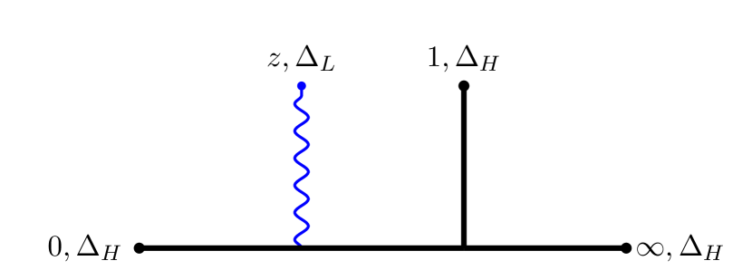
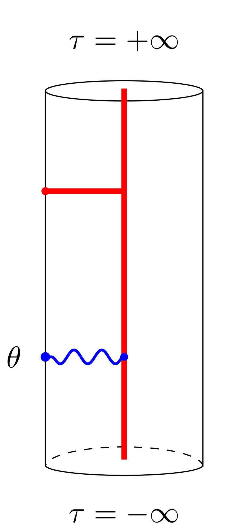
Figure 1: The 4-point HHHL block and its holographically dual realization in the three dimensional bulk (a rigid cylinder). The red lines inside the cylinder visualize the 3-point function $\langle\mathcal{O}_{H}\mathcal{O}_{H}\mathcal{O}_{H}\rangle$ of heavy operators that created this conical defect geometry. The wavy blue line denotes the perturbative operator $\mathcal{O}_{L}$ propagating in the background.

The operator $\mathcal{O}_{L}(z,\bar{z})$ is represented as the geodesic line stretched from the conformal boundary to a distinguished point in the bulk, see Fig. 1. Then, the geodesic length calculates the large-$c$ conformal block of the HHHL correlation function (1.1) in the first order of the perturbative expansion (1.2).

The paper is organized as follows. In Section 2 we calculate the large-$c$ 4-point block within the heavy-light perturbation theory using the monodromy method. In Section 3.1, based on the Bañados metric of locally AdS₃ spaces, we discuss different coordinate systems in the bulk induced by the boundary conformal (Schwarz) maps. Section 3.2 explicitly re-considers the known case of the 3-point function with two heavy insertions and shows that the block is calculated by the geodesic length of the boundary-to-bulk line. Section 3.3 follows the same patter and shows that the geodesic segment in the geometry created by three heavy insertions calculates the 4-point perturbative block found in Section 2.4. In the concluding Section 4 we propose how to generalize the obtained results to higher-point conformal blocks with more than three background operators.

2 Perturbative large-$c$ conformal blocks

Let us consider primary operators $\mathcal{O}_{i}$ in the plane CFT₂ with conformal dimensions $(\Delta_{i},\bar{\Delta}_{i})$, $i=1,...,4$. The 4-point correlation function in the $s$-channel can be expanded into conformal blocks [14]

$$\langle\mathcal{O}_{1}(0)\mathcal{O}_{2}(z,\bar{z})\mathcal{O}_{3}(1)\mathcal{O}_{4}(\infty)\rangle=\sum_{p}C_{12p}C_{34p}\,\mathcal{F}_{p}(z)\bar{\mathcal{F}}_{p}(\bar{z})\;,$$ (2.1)

where $C_{ijp}$ are structure constants, the (holomorphic) conformal blocks $\mathcal{F}_{p}(z)=\mathcal{F}(z|\Delta_{i},\Delta_{p},c)$ in a given channel $p$ depend on external $\Delta_{i}$, $i=1,...,4$ and intermediate $\Delta_{p}$ conformal dimensions, and on the central charge $c$, see Appendix A.

We consider the large central charge $c\to\infty$. Suppose that all the primary operators are heavy, i.e. their conformal dimensions grow linearly with the charge, $\Delta_{i}/c$ are fixed. Then, the 4-point block is exponentiated as

$$\mathcal{F}(z|\Delta_{i},\Delta_{p},c)\;\approx\;\exp{\frac{c}{6}f(z|\epsilon_{i},\epsilon_{p})}\quad\text{at}\quad c\to\infty\;,$$ (2.2)

where $f(z|\epsilon_{i},\epsilon_{p})$ is the classical conformal block depending on external and intermediate classical dimensions $\epsilon_{i}=6\Delta_{i}/c$ and $\epsilon_{p}=6\Delta_{p}/c$ [15].

The large-$c$ conformal blocks (2.2) can be calculated using the monodromy method. To this end, one considers the BPZ equation for the 5-point correlation function

$$\langle\mathcal{O}_{1}(0,0)\mathcal{O}_{2}(z,\bar{z})\Psi(y,\bar{y})\mathcal{O}_{3}(1,1)\mathcal{O}_{4}(\infty,\infty)\rangle\;,$$ (2.3)

obtained from the original function (2.1) by inserting the degenerate operator $\Psi(y,\bar{y})$ of conformal dimension $\Delta_{(1,2)}=-\frac{1}{2}-\frac{9}{2c}$ in some point $(y,\bar{y})\in\mathbb{C}$ [14]. Contrary to the original heavy operators this new operator is light because $\Delta_{(1,2)}=\mathcal{O}(c^{0})$ at $c\to\infty$. Now, the 5-point correlation function (2.3) can be expanded into conformal blocks in the OPE channel when the degenerate operator is inserted between two intermediate channels. The resulting 5-point conformal block is $\mathcal{V}(y,z|\Delta_{i},\Delta_{(1,2)},\Delta_{p},\Delta_{k},c)$, where the intermediate dimensions are related by the fusion relation $\Delta_{p}-\Delta_{k}=-\frac{9}{2c}\pm\frac{1}{2}\sqrt{1-\frac{24\Delta_{p}}{c}}$.

In the large-$c$ limit, the fusion rules claim that the 5-point block factorizes into the original 4-point block $\mathcal{F}(z|\Delta_{i},\Delta_{p},c)$ and a bi-local prefactor $\psi(z,y)$ as

$$\mathcal{V}(y,z|\Delta_{i},\Delta_{(1,2)},\Delta_{p},c)\;\approx\;\psi(y,z)\exp\left[\frac{c}{6}f(z|\epsilon_{i},\epsilon_{p})\right]\quad\text{at}\quad c\to\infty\;,$$ (2.4)

where we have taken into account that the 4-point block can be exponentiated (2.2).

From the BPZ equation for the original 5-point conformal block (2.4) one finds that the prefactor $\psi(y,z)$ satisfies the Fuchsian equation

$$\left[\frac{d^{2}}{dy^{2}}+T(y,z)\right]\psi(y,z)=0\;,$$ (2.5)

with the energy-momentum tensor of the form

$$T(y,z)=\frac{\epsilon_{1}}{y^{2}}+\frac{\epsilon_{2}}{(y-z)^{2}}+\frac{\epsilon_{3}}{(1-y)^{2}}+\frac{\epsilon_{4}-\epsilon_{3}-\epsilon_{1}-\epsilon_{2}}{(y-1)y}+c_{2}\,\frac{(1-z)z}{y(1-y)(y-z)}\;,$$ (2.6)

where the accessory parameter is expressed by

$$c_{2}=\frac{d}{dz}f(z|\epsilon_{i},\epsilon_{p})\;.$$ (2.7)

Note that there are three more accessory parameters associated to the point $0,1,\infty$ along with the energy-momentum tensor explicitly depending on them. However, recalling that $T\sim z^{-4}$ at infinity we can isolate the only independent accessory parameter $c_{2}$ so that the resulting $T$ is given by (2.6).

The monodromy method considers the Fuchsian equation (2.5) with a priori independent accessory parameter having no link to the 4-point conformal block. Comparing monodromy matrices of the original 5-point block and solutions to the Fuchsian equation yields the algebraic equation on the accessory parameter that expresses $c_{2}$ as a function of coordinates and conformal dimensions. Then, recalling the relation (2.7) we can explicitly integrate to obtain the 4-point large-$c$ conformal block.

2.1 Perturbative expansion

Suppose that the conformal dimensions are organized as follows

$$\Delta_{2}/\Delta_{1,3,4}\ll 1\quad\text{and}\quad\Delta_{1}\sim\Delta_{3}\sim\Delta_{4}\;,$$ (2.8)

i.e. there are three background operators with dimensions of the same order and one perturbative operator. In this way we obtain the correlation function of the type (1.1) – (1.2).

Assuming (2.8) the Fuchsian equation (2.5) - (2.7) can be explicitly solved by expanding all functions up to the first order in $\Delta_{2}$ as

$$\begin{gathered}\psi(y,z)=\psi^{(0)}(y,z)+\psi^{(1)}(y,z)+...\,,\qquad T(y,z)=T^{(0)}(y,z)+T^{(1)}(y,z)+...\,,\\ f(z|\epsilon,\epsilon_{p})=f^{(0)}(z|\epsilon,\epsilon_{p})+f^{(1)}(z|\epsilon,\epsilon_{p})+...\,,\qquad c_{2}(z|\epsilon,\epsilon_{p})=c_{2}^{(0)}(z|\epsilon,\epsilon_{p})+c_{2}^{(1)}(z|\epsilon,\epsilon_{p})+...\,.\end{gathered}$$ (2.9)

A few comments are in order. The term $f^{(0)}=0$ because the conformal block for the 3-point function $\langle\mathcal{O}_{H}(0)\mathcal{O}_{H}(1)\mathcal{O}_{H}(\infty)\rangle$ is equal to 1 that directly follows from (A.5). The zeroth order accessory parameter is also zero, $c_{2}^{(0)}(z|\epsilon,\epsilon_{p})=0$. Since we will consider only first-order corrections then the notations can be simplified by denoting $c_{2}^{(1)}(z|\epsilon,\epsilon_{p})\equiv c_{2}(z|\epsilon,\epsilon_{p})$.

The Fuchsian equation in the lowest orders takes the form

$$\left[\frac{d^{2}}{dy^{2}}+T^{(0)}(y)\right]\psi^{(0)}(y,z) =0\;,$$ (2.10)

$$\left[\frac{d^{2}}{dy^{2}}+T^{(0)}(y)\right]\psi^{(1)}(y,z) =-T^{(1)}(y,z)\psi^{(0)}(y,z)\;,$$ (2.11)

where the zeroth-order energy-momentum tensor $T^{(0)}(y)$ and the first-order correction $T^{(1)}(y)$ are given by

$$T^{(0)}(y) =\frac{\epsilon_{1}}{y^{2}}+\frac{\epsilon_{3}}{(1-y)^{2}}+\frac{\epsilon_{1}+\epsilon_{3}-\epsilon_{4}}{y(1-y)}\;,$$ (2.12)

$$T^{(1)}(y,z) =c_{2}\,\frac{(1-z)z}{y(1-y)(y-z)}+\frac{\epsilon_{2}}{(y-z)^{2}}+\frac{\epsilon_{2}}{y(1-y)}\;.$$ (2.13)

Note that $T^{(1)}(y,z)$ is indeed the first order correction because $c_{2}=\mathcal{O}(\epsilon_{2})$.

2.2 First-order solution

The zeroth-order Fuchsian equation (2.10) can be reduced to the hypergeometric equation in the so-called Q-form [22]. The parameters of the resulting hypergeometric function are expressed in terms of the conformal dimensions $\epsilon_{i}$ and $\epsilon_{p}$. To simplify the further analysis we assume that

$$\Delta_{3}=\Delta_{4}\;.$$ (2.14)

Moreover, this condition is required when considering going from three to two background operators. There are two branches of the zeroth-order solution,

$$\psi^{(0)}_{\pm}(y)=(1-y)^{\frac{1+\alpha}{2}}y^{\frac{1\pm\beta}{2}}F_{\pm}(\alpha,\beta|y)\,,$$ (2.15)

where the hypergeometric functions are given by

$$F_{\pm}(\alpha,\beta|y)={}_{2}F_{1}\left(\frac{1\pm\beta}{2},\frac{1\pm\beta}{2}+\alpha,1\pm\beta,y\right)\,,$$ (2.16)

and

$$\alpha=\sqrt{1-\frac{24\Delta_{4}}{c}}\;,\qquad\beta=\sqrt{1-\frac{24\Delta_{1}}{c}}\;,\qquad\;\;0<\alpha,\beta<1\;.$$ (2.17)

Consider then the Fuchsian equation in the first order (2.11). Using the method of variation of parameters we find the first order correction,

$$\psi^{(1)}_{\pm}(y,z)=\psi^{(0)}_{+}(y)\int dy\frac{\psi^{(0)}_{-}T^{(1)}(y,z)\psi^{(0)}_{\pm}}{W}-\psi^{(0)}_{-}(y)\int dy\frac{\psi^{(0)}_{+}T^{(1)}(y,z)\psi^{(0)}_{\pm}}{W}\;,$$ (2.18)

where the Wronskian is given by

$$W\equiv-\psi^{(0)}_{+}(y)\frac{d\psi^{(0)}_{-}}{dy}+\psi^{(0)}_{-}(y)\frac{d\psi^{(0)}_{+}}{dy}=\frac{\sin\pi\beta}{\pi}\;.$$ (2.19)

Thus, the first-order solution reads as $\psi_{\pm}(y,z)=\psi_{\pm}^{(0)}(y,z)+\psi_{\pm}^{(1)}(y,z)$, where $\psi_{\pm}^{0}$ and $\psi_{\pm}^{1}$ are given by (2.15) and (2.18). It is parameterized by the background dimensions (through $\alpha,\beta$) and depends on the indeterminate accessory parameter $c_{2}$.

2.3 More on the zeroth-order solution

When solving the second-order Fuchsian equation we can equally choose a linear combination of the solutions $\psi_{\pm}$. In particular, in the zeroth order,

$$\psi^{(0)}_{i}(y)\rightarrow\hat{\psi}^{(0)}_{i}(y)=A_{ij}\psi^{(0)}_{j}(y)\;,\qquad$$ (2.20)

where $i,j=+,-$ and $A_{ij}$ is a non-degenerate $[2\times 2]$ matrix. Let $A_{ij}=\begin{pmatrix}\alpha&1\\ 0&1\end{pmatrix}$. Expanding the resulting solution in powers of $\epsilon_{1}$ we find that

$$\hat{\psi}^{(0)}_{\pm}(y)=(1-y)^{\frac{1\pm\alpha}{2}}+\mathcal{O}(\epsilon_{1})\;.$$ (2.21)

In this way, we reproduce the case of two background operators [2] obtained here by sending $\epsilon_{1}\to 0$. Indeed, operators $\mathcal{O}_{1,2}$ in the 4-point correlation function (2.1) are now perturbatively light compared to $\mathcal{O}_{3,4}$ and the heavy-light perturbative expansion assumes that in the zeroth order $\epsilon_{1}=\epsilon_{2}=0$. Then, having started with the original $5$-point correlation function (2.3) now we are left with the 3-point function of the form

$$\langle\Psi_{(1,2)}(y,\bar{y})\mathcal{O}_{H}(1)\mathcal{O}_{H}(\infty)\rangle\;.$$ (2.22)

The BPZ equation for (2.22) in the large-$c$ limit is just the Fuchsian equation (2.10), (2.12) taken at $\epsilon_{3}=\epsilon_{4}$ and $\epsilon_{1}=0$. On the other hand, the BPZ equation is solved by functions $(1-y)^{\frac{1\pm\alpha}{2}}$ (see e.g. [23]). Thus, the functions $\psi^{(0)}$ are identified with 3-point degenerate conformal block.

Let us now consider the present case of three background operators. In the zeroth order, when $\Delta_{2}=0$, we obtain from (2.3) the 4-point function

$$\langle\Psi_{(1,2)}(y,\bar{y})\mathcal{O}_{H}(0)\mathcal{O}_{H}(1)\mathcal{O}_{H}(\infty)\rangle\;.$$ (2.23)

Since the operator $\Psi_{(1,2)}$ is degenerate (on the second level) then the associated BPZ equation for the degenerate 4-point conformal block in the $s$-channel reads [14]

$$\left[\frac{3}{4\Delta_{(1,2)}+2}\frac{d^{2}}{dy^{2}}+\frac{2-4y}{y(1-y)}\frac{d}{dy}+\frac{\Delta_{1}+\Delta_{3}-\Delta_{4}+\Delta_{(1,2)}}{y(y-1)}-\frac{\Delta_{1}}{y^{2}}-\frac{\Delta_{3}}{(1-y)^{2}}\right]\mathcal{F}(y|\Delta_{1,3,4},\Delta_{p},c)=0\;.$$ (2.24)

It is well known that the solution is given by the hypergeometric functions. In the large-$c$ regime we rescale the dimensions and notice then that the second term in (2.24) is small compared to the others. The resulting equation takes the form

$$\left[\frac{d^{2}}{dy^{2}}+\frac{\epsilon_{1}}{y^{2}}+\frac{\epsilon_{3}}{(1-y)^{2}}+\frac{\epsilon_{3}+\epsilon_{1}-\epsilon_{4}}{y(1-y)}\right]\mathcal{F}(y|\epsilon_{1,3,4},\epsilon_{p})=0\;.$$ (2.25)

This equation coincides with the zeroth-order Fuchsian equation (2.10), (2.12). Thus, the zeroth-order solution $\psi^{(0)}$ is the $4$-point degenerate conformal block.

2.4 Accessory parameters and the conformal block

Let us consider a contour $\Gamma$ enclosing points $0$ and $z$, and calculate the corresponding monodromy of the first order solution $\psi_{\pm}(y,z)=\psi_{\pm}^{(0)}(y,z)+\psi_{\pm}^{(1)}(y,z)$. The monodromy matrix $M=||M_{ij}||$ is $[2\times 2]$ matrix, $i=(+,-)$, that can be decomposed as

$$M_{ij}=M_{ij}^{(0)}+M_{ij}^{(1)}+...\;,$$ (2.26)

where the zeroth and the first order terms are given by

$$M^{(0)}=-\begin{pmatrix}e^{i\pi\beta}&0\\ 0&e^{-i\pi\beta}\end{pmatrix}\,,\qquad M^{(1)}=-\begin{pmatrix}e^{i\pi\beta}I_{++}\;\;&e^{-i\pi\beta}I_{+-}\\ e^{i\pi\beta}I_{-+}\;\;&e^{-i\pi\beta}I_{--}\end{pmatrix}\,,$$ (2.27)

where

$$I_{+\pm}=\frac{\pi}{\sin(\pi\beta)}\int_{\Gamma}dy\;\psi^{(0)}_{-}T^{(1)}(y,z)\psi^{(0)}_{\pm}\;,\qquad I_{-\pm}=-\frac{\pi}{\sin(\pi\beta)}\int_{\Gamma}dy\;\psi^{(0)}_{\pm}T^{(1)}(y,z)\psi^{(0)}_{-}\;.$$ (2.28)

Denoting $X=z(c_{2}(1-z)-2\epsilon_{2})+\epsilon_{2}(1-\alpha z)$ and $Y=X-\epsilon_{2}\beta(1-z)$, the contour integrals can be represented in the form

$$\begin{array}[]{l}\hskip 19.91692pt\displaystyle I_{++}=\frac{2i\pi^{2}(1-z)^{\alpha}F_{+}F_{-}}{\sin\pi\beta}\left(X+\epsilon_{2}z(1-z)\frac{d\log(F_{+}F_{-})}{dz}\right)\;,\\ \\ \displaystyle I_{+-}=-\frac{2i\pi^{2}(1-z)^{\alpha}z^{-\beta}F_{-}F_{-}}{\sin\pi\beta}\left(Y+\epsilon_{2}z(1-z)\frac{d\log(F_{-}F_{-})}{dz}\right)\;,\end{array}$$ (2.29)

and

$$I_{--}=-I_{++}\;,\qquad I_{-+}=I_{+-}\big{|}_{\beta\to-\beta}\;,$$ (2.30)

where $F_{\pm}$ are given in (2.16).

On the other hand, traversing the degenerate operator $\Psi_{(1,2)}(y,\bar{y})$ along the contour $\Gamma$, i.e. around the primary operators $\mathcal{O}(0)$ and $\mathcal{O}(z,\bar{z})$ we find that the respective monodromy is diagonal. Since the $5$-point block (2.4) has two independent components, the monodromy matrix $\widetilde{M}=||\widetilde{M}_{ij}||$ is also $[2\times 2]$, $i=(+,-)$. Taking the large-$c$ limit and calculating the matrix along the contour $\Gamma$ we find an exact expression

$$\widetilde{M}=-\begin{pmatrix}e^{i\pi\gamma}&0\\ 0&e^{-i\pi\gamma}\end{pmatrix},\qquad\;\;\gamma=\sqrt{1-\frac{24\Delta_{p}}{c}}\;,\qquad 0<\gamma<1\;,$$ (2.31)

which is valid in any order of our perturbation theory.

The two monodromy matrices $M$ (2.26) and $\widetilde{M}$ (2.31) describe the same monodromy and, therefore, have equal eigenvalues. The matrix $\widetilde{M}$ is already diagonal. To diagonalize $M$ we consider the corresponding characteristic equation

$$(\exp[i\pi\beta](1+I_{++})-\lambda)(\exp[-i\pi\beta](1-I_{++})-\lambda)-I_{+-}I_{-+}=0\;,$$ (2.32)

which has two complex conjugated roots

$$\lambda_{\pm}=-\frac{\exp[i\pi\beta](1+I_{++})+\exp[-i\pi\beta](1-I_{++})\pm i\sqrt{-D}}{2}\;,$$ (2.33)

with discriminant

$$D=(\exp[i\pi\beta](1+I_{++})+\exp[-i\pi\beta](1-I_{++}))^{2}-4+4(I^{2}_{++}+I_{+-}I_{-+})\;.$$ (2.34)

In order to compare the eigenvalues $\lambda_{\pm}$ with those of (2.31) one expands in powers of $\epsilon_{2}$. Since the monodromy integrals are linear in $\epsilon_{2}$ (recall that $c_{2}$ in $I_{++}$ is the first order correction, see our comment below (2.9)) we get in the first order,

$$\begin{gathered}\lambda_{+}=-e^{i\pi\beta}\left(1+I_{++}\right)+\mathcal{O}(\epsilon_{2}^{2})\;,\\[5.0pt] \lambda_{-}=-e^{-i\pi\beta}\left(1-I_{++}\right)+\mathcal{O}(\epsilon_{2}^{2})\;,\end{gathered}$$ (2.35)

that must be equal to $-e^{\pm i\pi\gamma}$. Equating order by order we obtain the following constraints

$$\gamma=\beta\;,\qquad I_{++}=0\;,$$ (2.36)

where $I_{++}$ is given in (2.29). From the first relation in (2.36) we find out that the first and the intermediate conformal dimensions must be equal,

$$\Delta_{p}=\Delta_{1}\;.$$ (2.37)

Such a condition is to be expected within the heavy-light perturbative expansion. By the fusion rules, when $\Delta_{2}=0$, the intermediate channel should be equated to the first primary insertion, thereby losing its own character just because the resulting 3-point function has no exchange channels.

Now, solving the second relation in (2.36) we obtain

$$c_{2}=\epsilon_{2}\left[\frac{1+\alpha}{1-z}-\frac{1}{z}-\frac{d\log(F_{+}F_{-})}{dz}\right]\;.$$ (2.38)

Integrating the defining relation (2.7) we find the 4-point perturbative classical conformal block with three background insertions

$$f(z|\alpha,\beta,\epsilon_{2})=-\epsilon_{2}\Big{(}\log(1-z)^{1+\alpha}+\log z+\log F_{+}(\alpha,\beta|z)+\log F_{-}(\alpha,\beta|z)\Big{)}\;,$$ (2.39)

where functions $F_{\pm}$ are given by (2.16).

A few comments are in order. First, in the limit $\beta\to 1$ corresponding to $\Delta_{1}\to 0$ we reproduce the 4-point perturbative block with two background operators at $\epsilon_{1}=\epsilon_{p}$ [3]. To this end, we decompose the function (2.39), where $\beta=\beta(\epsilon_{1})$ is given by (2.17), in powers of $\epsilon_{1}$ and keep the linear terms (see also Appendix A). Secondly, we note that when calculating the monodromy matrix $M$ we could equally use solutions (2.20). In this case, the resulting monodromy matrix is related to (2.26) by $\hat{M}=AMA^{-1}$ and, therefore, the eigenvalue problem remains the same giving rise to the same accessory parameter and conformal block.

3 Holographically dual description

In this section we develop the holographic interpretation of the large-$c$ perturbative conformal blocks with three background operators. For two background operators the respective blocks were realized as geodesic trees in the conical defect space parameterized by $\alpha=\alpha(\Delta_{H})$ (2.17).

3.1 Conformal maps and the bulk metrics

In the AdS₃/CFT₂ correspondence, the locally AdS₃ geometry created by heavy insertions of the boundary CFT can be described in the Bañados form [24]

$$ds^{2}=R^{2}\left(-Hdz^{2}-\bar{H}d\bar{z}^{2}+\frac{u^{2}}{4}\,H\bar{H}\,dzd\bar{z}+\frac{du^{2}+dzd\bar{z}}{u^{2}}\right)\;,$$ (3.1)

with $u\in[0,\infty)$ and $z,\bar{z}\in\mathbb{C}$ being local coordinates, the radius is $R$. Arbitrary (anti)holomorphic functions $H=H(z)$ and $\bar{H}=\bar{H}(\bar{z})$ can be interpreted as components of the holographic CFT₂ energy-momentum tensor

$$T(z)=\frac{c}{6}H(z)\;,$$ (3.2)

where the central charge is $c=3R/2G_{N}$ [25, 26]. Under $z\to w(z)$ it transforms in the standard fashion as

$$T(z)=\left(w^{\prime}\right)^{2}T(w)+\frac{c}{12}\,\{w,z\}\;,\qquad\text{where}\quad\{w,z\}=\frac{w^{\prime\prime\prime}}{w^{\prime}}-\frac{3}{2}\left(\frac{w^{\prime\prime}}{w^{\prime}}\right)^{2}\;,$$ (3.3)

where the prime denotes differentiation with respect to $z$. The anti-holomorphic component transforms analogously.

Let us find a map $z\to w(z)$ such that $H(w(z))=0$. Away from singularities it would correspond to pure AdS₃ in the Poincare coordinates, cf. (3.1). This can be achieved provided that

$$H(z)=\frac{1}{2}\{w,z\}\;.$$ (3.4)

The solution to the above equation can be represented as the ratio of two independent solutions to the auxiliary Fuchsian equation $\psi^{{}^{\prime\prime}}+H\psi=0$ (see e.g. [22]). This is the so-called Schwarz map

$$w(z)=\frac{A\,\psi_{1}(z)+B\,\psi_{2}(z)}{C\,\psi_{1}(z)+D\,\psi_{2}(z)}\equiv\frac{A\,\frac{\psi_{1}(z)}{\psi_{2}(z)}+B}{C\,\frac{\psi_{1}(z)}{\psi_{2}(z)}+D}\;,\qquad AD-BC\neq 0\;,$$ (3.5)

where $\psi_{1,2}$ are two independent Fuchsian solutions, and $A,B,C,D\in\mathbb{C}$ parameterize the Möbius transformation of $\psi_{1}(z)/\psi_{2}(z)$.

The relation (3.2) and the Fuchsian interpretation of solutions to the equation (3.4) suggest that in the large-$c$ regime the function $H$ can be identified with the classical energy-momentum tensor arising in the Fuchsian equation (2.10) of the monodromy method, i.e.,

$$H(z|{\bf z})\equiv T^{(0)}(z|{\bf z})\;,$$ (3.6)

where we introduced the set of singular points ${\bf z}$ identified with locations of the background operators.

Since any solution to the Einstein equations with the (negative) cosmological constant is locally AdS₃ space then the boundary map (3.5) can be extended to the whole three-dimensional space, $w=w(z,\bar{z},u)$, $\bar{w}=\bar{w}(z,\bar{z},u)$, and $v=v(z,\bar{z},u)$, such that the resulting metric describes the Poincare patch

$$d\tilde{s}^{2}=\frac{dv^{2}+dwd\bar{w}}{v^{2}}\;.$$ (3.7)

The explicit coordinate transformation reads [27]

$$\begin{gathered}\displaystyle w(z,\bar{z},u)=w(z)-\frac{2u^{2}w^{\prime}(z)^{2}\bar{w}^{\prime\prime}(\bar{z})}{4w^{\prime}(z)\bar{w}^{\prime}(\bar{z})+u^{2}w^{\prime\prime}(z)\bar{w}^{\prime\prime}(\bar{z})}\;,\\[5.0pt] \displaystyle\bar{w}(z,\bar{z},u)=\bar{w}(\bar{z})-\frac{2u^{2}\bar{w}^{\prime}(\bar{z})^{2}w^{\prime\prime}(z)}{4w^{\prime}(z)\bar{w}^{\prime}(\bar{z})+u^{2}w^{\prime\prime}(z)\bar{w}^{\prime\prime}(\bar{z})}\;,\\[5.0pt] \displaystyle v(z,\bar{z},u)=u\,\frac{4\left(w^{\prime}(z)\bar{w}^{\prime}(\bar{z})\right)^{3/2}}{4w^{\prime}(z)\bar{w}^{\prime}(\bar{z})+u^{2}w^{\prime\prime}(z)\bar{w}^{\prime\prime}(\bar{z})}\;.\end{gathered}$$ (3.8)

The length of a geodesic line stretched between two points $(w_{1},\bar{w}_{1},v_{1})$ and $(w_{2},\bar{w}_{2},v_{2})$ evaluated in the Poincare coordinates (3.7) is particularly simple

$$\mathcal{L}_{{}_{AdS}}=R\log\frac{(w_{1}-w_{2})(\bar{w}_{1}-\bar{w}_{2})}{v_{1}v_{2}}\;.$$ (3.9)

Finally, we note that in the Euclidean case the Poincare patch covers the whole global AdS${}_{3}\;$space

$$d\hat{s}^{2}=\frac{d\tau^{2}+d\rho^{2}+\sin^{2}\rho d\phi^{2}}{\cos^{2}\rho}\;.$$ (3.10)

through the coordinate change $w=e^{\theta}\sin\rho$, $\bar{w}=e^{\bar{\theta}}\sin\rho$, $v=e^{\frac{\theta+\bar{\theta}}{2}}\cos\rho$, where $\theta=\tau+i\phi$ and $\rho$ are coordinates of the global AdS₃ (rigid cylinder). The conformal boundary is at $\rho=\pi/2$. There is a conformal map $\theta=\log w$ from the boundary $(w,\bar{w})$-plane to the boundary $(\theta,\bar{\theta})$-cylinder.

3.2 3-point HHL block as geodesic length

Let us first consider the simplest case of 3-point function with two background insertions in $1$ and $\infty$, see (A.3). The classical energy-momentum tensor (3.6) is given by

$$T^{(0)}(z)=\frac{\epsilon_{3}}{(1-z)^{2}}\;,$$ (3.11)

where $\epsilon_{2}=\epsilon_{3}$ are classical dimensions of the background operators. It follows that there are two lines of coordinate singularities in the Bañados metric (3.1): $(z,\bar{z},u)=(1,1,u)$ and $(z,\bar{z},u)=(\infty,\infty,u)$ at $\forall u\in\mathbb{R}_{+}$. The resulting space will be denoted as AdS${}_{3}[2]$.

Modulo Möbius transformations, the conformal mapping (3.5) is given by

$$w(z)=(1-z)^{\alpha}\;,$$ (3.12)

where we used the Fuchsian solution (2.21) and $\alpha$ is given by (2.17). The function $w(z)$ has two singular points $1$ and $\infty$, corresponding to locations of the background operators. It maps the $(z,\bar{z})$-plane onto the $(w,\bar{w})$-plane with an angle deficit proportional to $\alpha\in(0,1)$, cf. (2.17). Near $z=\infty$ we can change $z\to 1/z$ so that $w(z)\approx z^{-\alpha}$. Thus, at infinity, there is an angle excess parameterized by $-\alpha$.

The Poincare coordinates in AdS₃[2] can be explicitly read off from (3.8) (see also [28])

$$w(z,u)=\;(1-z)^{\alpha}\;\frac{(1-\alpha^{2})u^{2}+4(1-z)(1-\bar{z})}{(1-\alpha)^{2}u^{2}+4(1-z)(1-\bar{z})}\;,$$ (3.13)

$$\bar{w}(\bar{z},u)=\;(1-\bar{z})^{\alpha}\;\frac{(1-\alpha^{2})u^{2}+4(1-z)(1-\bar{z})}{(1-\alpha)^{2}u^{2}+4(1-z)(1-\bar{z})}\;,$$ (3.14)

$$\displaystyle v(z,\bar{z},u)=\;4\alpha\;\frac{u(1-z)^{\frac{1+\alpha}{2}}(1-\bar{z})^{\frac{1+\alpha}{2}}}{(1-\alpha)^{2}u^{2}+4(1-z)(1-\bar{z})}\;.$$ (3.15)

Near the singular points the map is approximated by $w=(1-z)^{\alpha}(1+\mathcal{O}(1-z))$ along with

$$z\to 1\;:\qquad v(z,\bar{z},u)=\;\frac{4\alpha\,u^{-1}}{(1-\alpha)^{2}}\;\left[(1-z)(1-\bar{z})\right]^{\frac{\alpha+1}{2}}(1+\mathcal{O}((1-z)(1-\bar{z})))\;,$$ (3.16)

$$z\to\infty\;:\qquad v(z,\bar{z},u)=\;\alpha\,u\;(z\bar{z})^{\frac{\alpha-1}{2}}(1+\mathcal{O}(1/(z\bar{z})))\;.$$ (3.17)

Since $\alpha\in(0,1)$ the leading exponent in the first relation above is positive, while in the second relation it is negative. Thus, the lines of coordinate singularities of the Bañados metric are mapped to two boundary points $(w,\bar{w},v)=(0,0,0)$ and $(w,\bar{w},v)=(\infty,\infty,0)$.

Further, when going to the global AdS${}_{3}\;$space (3.10) both singularities are mapped to the boundary points $\tau=\pm\infty$. The coordinate $\phi$ is rescaled by $\alpha$ so that we have a wedge-shaped sector cut from the cylinder and the remaining domain is $\phi\in[0,2\pi\alpha)$, $\tau\in\mathbb{R}$, $\rho\in\mathbb{R}_{+}$. This is the standard conical defect in the AdS${}_{3}\;$space.

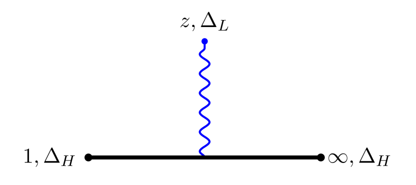
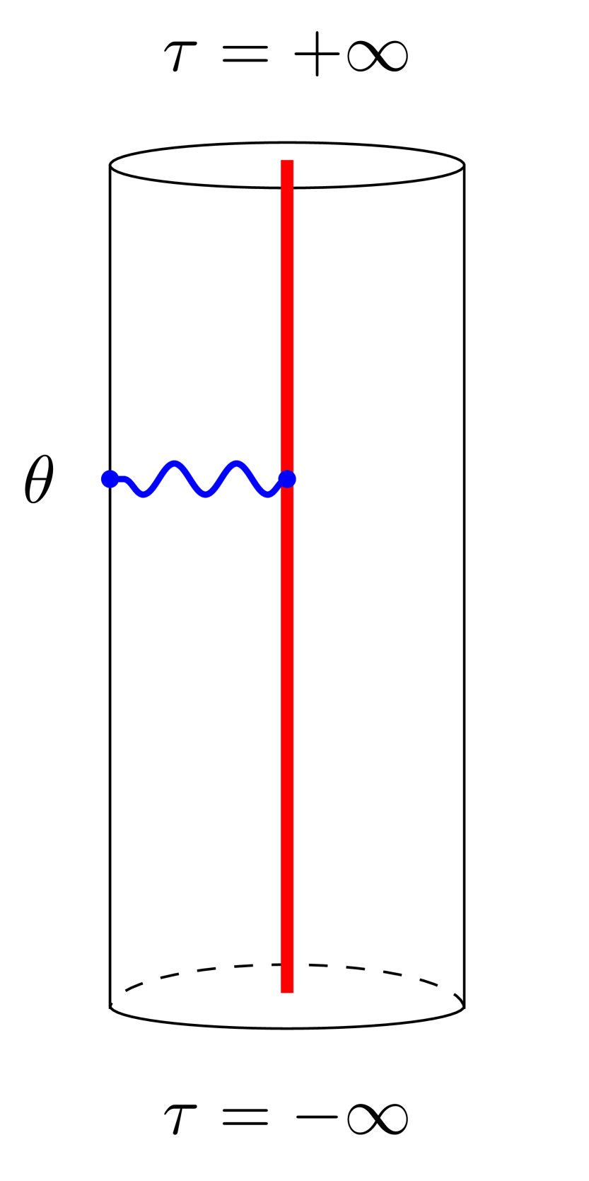
Figure 2: The 3-point HHL block and its holographically dual realization in the three dimensional bulk (a rigid cylinder). The red line along the cylinder axis visualizes the 2-point function $\langle\mathcal{O}_{H}\mathcal{O}_{H}\rangle$ of heavy operators inserted at infinities that produced the conical defect. The wavy blue line denotes the perturbative operator $\mathcal{O}_{L}$ propagating in the background.

Now we consider the 3-point conformal block, which in the original coordinates is given by

$$f(z|\epsilon_{1})=-\epsilon_{1}\log(1-z)\;,$$ (3.18)

see eq. (A.5). The perturbative operator of classical dimension $\epsilon_{1}$ is inserted in $(z,\bar{z})$.

To find the block function in different coordinate systems we recall the relation (A.2). In our case, the transformation from some $x$-coordinates to $y$-coordinates takes the form

$$f(x)=f(y(x))+\epsilon_{1}\log y^{\prime}(x)\;,$$ (3.19)

where the prime denotes differentiation with respect to $x$. Keeping only coordinate-dependent terms (this is $\sim$ below) we find that the block function in three coordinate systems on the boundary (original $(z,\bar{z})$, then conformally mapped $(w,\bar{w})$, and global $(\theta,\bar{\theta})$) is given by

$$f(z|\epsilon_{1})\sim-\epsilon_{1}\log\frac{w(z)}{w^{\prime}(z)}\;,\qquad f(w|\epsilon_{1})\sim-\epsilon_{1}\log w\;,\qquad f(\theta|\epsilon_{1})\sim 0\;.$$ (3.20)

Let us consider the AdS${}_{3}[2]$ space in the Poincare coordinates and fix two points: the boundary insertion of the perturbative operator $(w,\bar{w},\varepsilon)$ and a distinguished point inside the bulk $(0,0,1)$, where $\varepsilon\to 0$ is the boundary cut-off. The point belongs to the line connecting two background insertions at infinities, see Fig. 2. Then, the geodesic length between these two points given by (3.9) takes the form

$$\mathcal{L}_{{}_{AdS_{{}_{3}}[2]}}(w,\bar{w})=R\left(\log w+\log\bar{w}\right)-R\log\varepsilon\;.$$ (3.21)

Comparing with (3.20) we find that in the Poincare coordinates, modulo $\varepsilon$-dependent terms and constants, the block function and the geodesic length are identified,

$$f(w|\epsilon_{1})\sim-\frac{\;\epsilon_{1}}{R}\;\mathcal{L}_{{}_{AdS_{{}_{3}}[2]}}(w)\;,$$ (3.22)

where we omitted the anti-holomorphic part corresponding to the anti-holomorphic conformal block. In the large-$c$ regime, the standard formula relating masses and heavy conformal dimensions takes the form $mR\sim\Delta$ so that the ratio $\epsilon_{1}/R$ measures the mass of a point particle propagating in AdS${}_{3}[2]$. This is the block/length identification in the case of 3-point block with two background operators [13].

In the global coordinates, the distinguished point turns to the axis $\rho=0$ of the rigid cylinder so that the geodesic line is stretched from the boundary point to the center, see Fig. 2. Its regulated length turns out to be zero, $\mathcal{L}_{{}_{AdS_{{}_{3}}[2]}}(\theta,\bar{\theta})\sim 0$, that agrees with $f(\theta)=0$ in (3.20).

Note that there is another possible geodesic line in the bulk with boundary endpoints corresponding to the CFT operators. It connects two boundary points and the geodesic length calculates the 4-point identity HHLL conformal block [1, 29, 30]. For conformal blocks with more perturbative insertions the dual geodesic network has several boundary attachments and one endpoint in the center of the cylinder. In that case both the total length and the perturbative blocks are non-vanishing satisfying the relation of the type (3.22) [3, 6, 7, 9, 13].

3.3 4-point HHHL block as geodesic length

Let us turn to the case of the background geometry created by three heavy insertions. Here, the classical energy-momentum tensor (3.6) is given by

$$T^{(0)}(z)=\frac{\epsilon_{1}}{z^{2}}+\frac{\epsilon_{3}}{(z-1)^{2}}+\frac{\epsilon_{1}}{z(1-z)}\;,$$ (3.23)

where $\epsilon_{1}$ and $\epsilon_{3}=\epsilon_{4}$ are classical dimensions of the heavy background insertions in $0,1,\infty$. The resulting space defined by the Bañados metric (3.1) will be denoted as AdS${}_{3}[3]$. There are three lines of coordinate singularities: $(z,\bar{z},u)=(0,0,u)$, $(z,\bar{z},u)=(1,1,u)$, and $(z,\bar{z},u)=(\infty,\infty,u)$ for any $u\in\mathbb{R}_{+}$.

Choosing in (3.5) the Fuchsian solutions as $\psi_{1,2}(z)=\psi_{\pm}^{(0)}(z)$ (2.15) we find that up to the Möbius transformations the conformal mapping is given by

$$w(z)=z^{\beta}\;\frac{{}_{2}F_{1}\left(\frac{1+\beta}{2},\frac{1+\beta}{2}+\alpha,1+\beta,z\right)}{{}_{2}F_{1}\left(\frac{1-\beta}{2},\frac{1-\beta}{2}+\alpha,1-\beta,z\right)}\;.$$ (3.24)

This is the Schwarz triangle function that maps the $(z,\bar{z})$-plane onto some curvilinear triangle on the $(w,\bar{w})$-plane (see e.g. [31]). Since the Möbius group acts triply transitively and conformally, then the vertices can be placed in any positions, while the angles remain intact. By construction, the Schwarz function has three singular points $z=0,1,\infty$ identified with background operator locations. The angles and verities of the triangle are expressed in terms of parameters $\alpha,\beta$ of the function (3.24). We find that the angle in the point $w(0)$ is equal to $\pi\beta$, the second angle in $w(1)$ is equal to $-\pi\alpha$, and the third angle in $w(\infty)$ is equal to $\pi\alpha$. Recalling the definition (2.17) we obtain that the sum of angles in the triangle is $\pi\beta<\pi$.

The Schwarz triangle function near the singular points can be approximated by

$$z\to 0: w(z)\sim z^{\beta}(1+\mathcal{O}(z))\;,$$ (3.25)

$$z\to 1: w(z)\sim(1-z)^{-\alpha}(1+\mathcal{O}(1-z))\;,$$

$$z\to\infty: w(z)\sim z^{-\alpha}(1+\mathcal{O}(1/z))\;,$$

where $\sim$ indicates that these expansions are valid modulo Möbius transformations. The leading exponents in (3.25) define the angle deficit/excess. The Schwarz triangle function (3.24) in the singular points is given by

$$w(0)=0\;,\qquad w(1)=\infty\;,\qquad w(\infty)=e^{i\pi\beta}\;\frac{\Gamma(1+\beta)\;\Gamma(\frac{1-\beta}{2}+\alpha)\;\Gamma(\frac{1-\beta}{2})}{\Gamma(1-\beta)\;\Gamma(\frac{1+\beta}{2}+\alpha)\;\Gamma(\frac{1+\beta}{2})}\;.$$ (3.26)

From the asymptotics (3.25) we can find how $v$-coordinate behaves near the singular points. Applying the general relations (3.8) we obtain

$$z\to 0\;:\qquad v(z,\bar{z},u)=\;\frac{4\beta\,u^{-1}}{(1-\beta)^{2}}\;(z\bar{z})^{\frac{1+\beta}{2}}(1+\mathcal{O}(z\bar{z}))\;,$$ (3.27)

$$z\to 1\;:\qquad v(z,\bar{z},u)=\;\frac{4\alpha\,u^{-1}}{(1+\alpha)^{2}}\;\left[(1-z)(1-\bar{z})\right]^{\frac{1-\alpha}{2}}(1+\mathcal{O}((1-z)(1-\bar{z})))\;,$$ (3.28)

$$z\to\infty\;:\qquad v(z,\bar{z},u)=\;\alpha\,u\;(z\bar{z})^{-\frac{1+\alpha}{2}}(1+\mathcal{O}(1/(z\bar{z})))\;.$$ (3.29)

Since $\alpha,\beta\in(0,1)$, then the leading exponents in the first two relations are positive, while in the third one it is negative. It follows that the three lines of coordinate singularities in the Bañados metric (3.1) are mapped to three boundary points in the Poincare metric which are vertices of the curvilinear triangle. In the global coordinates, they lie on the boundary cylinder $\rho=\pi/2$ at $\theta_{0,1}=\pm\infty$ and $\theta_{\infty}=\log w_{\infty}$, where $w_{\infty}$ is given in (3.26), see Fig. 1.

Let us consider now the conformal block (2.39) in three boundary coordinate systems: $(z,\bar{z})$-plane, $(w,\bar{w})$-domain, $(\theta,\bar{\theta})$-cylinder discussed in Section 3.1. Assuming that we do some coordinate change $x\to x(y)$ the transformation formula (A.2) takes the form

$$f(x|\alpha,\beta,\epsilon_{2})=f(y(x)|\alpha,\beta,\epsilon_{2})+\epsilon_{2}\log y^{\prime}(x)\;.$$ (3.30)

Differentiating the Schwarz triangle function (3.24) and using the Wronskian (2.19) one finds that

$$w^{\prime}(z)=\frac{\sin\pi\beta}{\pi}\,\frac{(1-z)^{-1-\alpha}z^{-1+\beta}}{F^{2}_{-}(\alpha,\beta|z)}\;,$$ (3.31)

where $F_{-}$ is given by (2.16). The block function (2.39) in three coordinate systems is given by

$$f(z|\alpha,\beta,\epsilon_{2})\sim-\epsilon_{2}\log\frac{w(z)}{w^{\prime}(z)}\;,\qquad f(w|\alpha,\beta,\epsilon_{2})\sim-\epsilon_{2}\log w\;,\qquad f(\theta|\alpha,\beta,\epsilon_{2})\sim 0\;,$$ (3.32)

where $\sim$ stands for constants terms, cf. (3.20).

The above relations suggest that the bulk interpretation of the 4-point block with three background operators is quite similar to that of 3-point block with two background operators. Indeed, according to our prescription we fix two points in AdS${}_{3}[3]$ in the Poincare coordinates: the boundary insertion of the perturbative operator $(w,\bar{w},\varepsilon)$ and the distinguished point in the bulk $(0,0,1)$, where the cut-off $\varepsilon\to 0$. The distinguished point belongs to the vertex joining the background heavy insertions: two at infinities, one in a finite region of the conformal boundary, see Fig. 1. Then, the geodesic length (3.9) is given by

$$\mathcal{L}_{{}_{AdS_{{}_{3}}[3]}}(w,\bar{w})=R\left(\log w+\log\bar{w}\right)-R\log\varepsilon\;,$$ (3.33)

and comparing with (3.32) we find that in this case the holomorphic block/length relation is

$$f(w|\alpha,\beta,\epsilon_{2})\sim-\frac{\;\epsilon_{2}}{R}\;\mathcal{L}_{{}_{AdS_{{}_{3}}[3]}}(w)\;,$$ (3.34)

where $\sim$ means up to constant and divergent contributions. The same relation holds in the global coordinates, where the both sides are vanishing, see the last relation in (3.32).

4 Concluding remarks: more than three background operators

By way of conclusion, let us briefly outline a possible generalization of the previous results. The 3-point and 4-point functions with respectively two and three background insertions belong to the general family of $n$-point large-$c$ functions with $n-k$ background operators. Let us denote them as H^n-kL^k type functions, where a true parameter is the number of perturbative operators $k$ measuring a deviation form the classical $n$-point block. The previously considered cases are, therefore, type H²L and $H^{3}L$ functions.

Let AdS${}_{3}[n-k]$ be a three-dimensional space with the Bañados metric defined by the classical energy-momentum tensor $T(z|{\bf z})$ with $n-k$ singular points. The boundary Schwarz mappings and the Poincare coordinates are build using the solutions of the associated Fuchsian equation,

$$\left[\frac{d^{2}}{dz^{2}}+T(z|{\bf z})\right]\psi(z)=0\;,\quad\text{where}\quad T(z|{\bf z})=\sum_{i=k+1}^{n}\frac{\epsilon_{i}}{(z-z_{i})^{2}}+\frac{c_{i}}{z-z_{i}}\;,$$ (4.1)

where ${\bf z}=(z_{k+1},...,z_{n})$ are locations of the background operators with classical dimensions $\epsilon_{i}$, the $c_{i}$ are respective accessory parameters. The resulting space AdS${}_{3}[n-k]$ will have $n-k$ conical defects parameterized by background conformal dimensions as can be directly seen from the Schwarz map of the $(z,\bar{z})$-plane to some curvilinear polygon with $n-k$ vertices on the $(w,\bar{w})$-plane.

Assuming that $\epsilon_{j}/\epsilon_{i}\ll 1$ for $j=1,...,k$ and $i=k+1,...,n$ we can use the heavy-light approximation and introduce type $H^{n-k}L^{k}$ perturbative conformal blocks $f_{(k,n-k)}(w)$. The point is that when we calculate such perturbative blocks using the monodromy method, the energy-momentum tensor arising in the zeroth order is exactly (4.1).

On the other hand, within the monodromy method the zeroth-order Fuchsian solutions are the degenerate $(n-k+1)$-point conformal blocks of the background operators taken in the large-$c$ limit, where the additional operator is the degenerate light $\Psi_{(1,2)}$, see Section 2.3. Thus, the auxiliary equation (4.1) responsible for the Schwarz mappings is the BPZ equation describing the degenerate background blocks $\psi(z)$.

It is tempting to conjecture that type $H^{n-k}L^{k}$ conformal blocks are equal to the length of dual Steiner trees in AdS${}_{3}[n-k]$,

$$f_{(k,n-k)}(w|\epsilon)\sim-\frac{1}{R}\;\mathcal{L}_{{}_{AdS_{{}_{3}}[n-k]}}(w|\epsilon)\;,$$ (4.2)

where the right-hand side is the weighted length of the dual tree, and $w$ are locations of perturbative operators in the Poincare coordinates which can be found from the general formula (3.8).

Acknowledgements. We are grateful to V. Belavin for useful exchanges. The work was supported by the Russian Science Foundation grant 18-72-10123.

Appendix A The lower-point conformal blocks: various details

Here, we discuss 3-point and 4-point conformal blocks in the context of the heavy-light expansion. All block functions are normalized as $\mathcal{F}\sim z^{\gamma}$ at $z\to 0$, where $\gamma$ is the linear combination of conformal dimensions. The other normalization $\mathcal{F}\sim 1$ is also possible, in which case, e.g. the decomposition (2.1) would explicitly contain $z^{\gamma}$ factors.

Conformal maps.

Under the map $z\rightarrow w(z)$ the $n$-point correlation functions of primary operators transform as (see e.g. [23])

$$\langle\mathcal{O}_{1}(w_{1})\cdots\mathcal{O}_{n}(w_{n})\rangle=\prod^{n}_{i=1}\left(\frac{dw}{dz}\right)^{-\Delta_{i}}_{w=w_{i}}\left(\frac{d\bar{w}}{d\bar{z}}\right)^{-\bar{\Delta}_{i}}_{\bar{w}=\bar{w}_{i}}\langle\mathcal{O}_{1}(z_{1})\cdots\mathcal{O}_{n}(z_{n})\rangle\;.$$ (A.1)

It follows that large-$c$ perturbative conformal block with $k$ perturbative and $n-k$ background operators transforms as

$$f(w_{1}(z),...,w_{k}(z)|\epsilon,\tilde{\epsilon})=f(z_{1},...,z_{k}|\epsilon,\tilde{\epsilon})-\sum_{i=1}^{k}\epsilon_{i}\log\frac{dw_{i}(z)}{dz_{i}}\;,$$ (A.2)

where $\epsilon,\tilde{\epsilon}$ are classical external and intermediate dimensions of the perturbative operators.

3-point conformal block.

In this case we have

$$\langle\mathcal{O}_{2}(z,\bar{z})\mathcal{O}_{2}(1)\mathcal{O}_{3}(\infty)\rangle=(\infty)^{2\Delta_{3}}C_{123}\,\mathcal{F}(z)\bar{\mathcal{F}}(\bar{z})\;,$$ (A.3)

where the (holomorphic) block can be defined as

$$\mathcal{F}(z)=(1-z)^{-(\Delta_{1}+\Delta_{2}-\Delta_{3})}\;.$$ (A.4)

The block function at arbitrary $z_{2}$ and $z_{3}$ can be similarly defined. Modulo infinite prefactors the correlation function (A.3) can be exponentiated to yield the 3-point classical conformal block

$$f(z|\epsilon)=-(\epsilon_{1}+\epsilon_{2}-\epsilon_{3})\log(1-z)\;,$$ (A.5)

where the classical dimensions are $\epsilon_{i}=6\Delta_{i}/c$. The 3-point function is exact within the heavy-light expansion.

4-point conformal block.

Here we reproduce the perturbative block (2.39) directly from the original Virasoro block in the large-$c$ and the heavy-light approximations. The $s$-channel block function can be expanded near $z=0$ as [14]

$$\mathcal{F}(z|\Delta_{i},\Delta_{p},c)=z^{\Delta_{p}-\Delta_{1}-\Delta_{2}}\sum_{N=0}^{\infty}F_{N}z^{N}\;,$$ (A.6)

where the expansion coefficients $F_{N}=F_{N}(\Delta_{i},\Delta_{p},c)$ in the lowest orders are given by

$$F_{0}=1\;,\qquad F_{1}=\frac{(\Delta_{p}-\Delta_{1}+\Delta_{2})(\Delta_{p}-\Delta_{4}+\Delta_{3})}{2\Delta_{p}}\;,$$ (A.7)

$$\begin{array}[]{c}\displaystyle F_{2}=\frac{(\Delta_{p}+\Delta_{2}-\Delta_{1})(\Delta_{p}+\Delta_{2}-\Delta_{1}+1)(\Delta_{p}+\Delta_{3}-\Delta_{4})(\Delta_{p}+\Delta_{3}-\Delta_{4}+1)}{4\Delta_{p}(2\Delta_{p}+1)}+\\ \\ \displaystyle+2\left(\frac{\Delta_{1}+\Delta_{2}}{2}+\frac{3(\Delta_{1}-\Delta_{2})^{2}}{2(1+2\Delta_{p})}+\frac{(\Delta_{p}-1)\Delta_{p}}{2(1+2\Delta_{p})}\right)\left(c+\frac{2\Delta_{p}(8\Delta_{p}-5)}{(1+2\Delta_{p})}\right)^{-1}\times\\ \\ \displaystyle\times\left(\frac{\Delta_{3}+\Delta_{4}}{2}+\frac{3(\Delta_{4}-\Delta_{3})^{2}}{2(1+2\Delta_{p})}+\frac{(\Delta_{p}-1)\Delta_{p}}{2(1+2\Delta_{p})}\right)\;.\end{array}$$ (A.8)

To calculate perturbative classical blocks, we do the following steps.

• The large-$c$ regime, the classical dimensions:

  $$\epsilon_{i,p}=6\Delta_{i,p}/c\;,\qquad i=1,2,3,4\;.$$ (A.9)

• The classical block (see (2.2)):

  $$f(z|\epsilon_{i},\epsilon_{p})\approx\frac{6}{c}\log\mathcal{F}(z|\Delta_{i},\Delta_{p},c)+\mathcal{O}(1/c)\;.$$ (A.10)

• The lightness parameter $\delta\ll 1$: rescale a part of conformal dimensions as $\epsilon_{i,p}\rightarrow\delta\epsilon_{i,p}$ and expand $f=f(z|\epsilon_{i},\epsilon_{p})$ in powers of $\delta$,

  $$f=\frac{1}{\delta^{s}}f_{-s}+\frac{1}{\delta^{s-1}}f_{-s+1}+...+\delta^{0}f_{0}+\delta f_{1}+\mathcal{O}(\delta^{2})\;,$$ (A.11)

  for some $s\in\mathbb{N}$. Since for general dimensions we have the Laurent series, we require that all singular terms $f_{-n}$ must be vanishing that imposes constraints on conformal dimensions. (For $n$-point blocks with two background operators this is $\epsilon_{3}=\epsilon_{4}$, for the 4-point block with three background operators this is $\epsilon_{1}=\epsilon_{p}$). The term $f_{0}$ is the leading (background) classical block. The perturbative block is defined to be the first correction $f_{1}$.

Having three heavy background operators we rescale $\epsilon_{2}\to\delta\epsilon_{2}$ and find the perturbative block

$$f_{1}=-\epsilon_{2}\log z+\epsilon_{2}\sum_{N=1}^{\infty}{\text{f}}_{N}z^{N}\;,$$ (A.12)

where

$${\text{f}}_{1}=\frac{1}{2}\;,\qquad{\text{f}}_{2}=\frac{3+8\epsilon_{1}+16\epsilon_{4}}{8(3+4\epsilon_{1})}\;.$$ (A.13)

Note that rescaling further $\epsilon_{1}\rightarrow\delta\epsilon_{1},\epsilon_{p}\rightarrow\delta\epsilon_{p}$ and decomposing again in powers of $\delta$, we get the coefficients of the perturbative HHHL block with $\epsilon_{1}=\epsilon_{p}$ [3].

On the other hand, the small-$z$ expansion (modulo logarithms) of the perturbative block (2.39) is given by the same (A.12), where the first coefficients are given by

$${\text{f}}_{1}=\frac{1}{2}\;,\qquad{\text{f}}_{2}=\frac{2\beta^{2}+4\alpha^{2}-9}{8(\beta^{2}-4)}\;.$$ (A.14)

Using the change (2.17) we can see that these coefficients coincide with (A.13).

References

- [1] C. T. Asplund, A. Bernamonti, F. Galli and T. Hartman, Holographic Entanglement Entropy from 2d CFT: Heavy States and Local Quenches, JHEP 1502 (2015) 171, [1410.1392].
- [2] A. L. Fitzpatrick, J. Kaplan and M. T. Walters, Universality of Long-Distance AdS Physics from the CFT Bootstrap, JHEP 1408 (2014) 145, [1403.6829].
- [3] E. Hijano, P. Kraus and R. Snively, Worldline approach to semi-classical conformal blocks, JHEP 07 (2015) 131, [1501.02260].
- [4] A. L. Fitzpatrick, J. Kaplan and M. T. Walters, Virasoro Conformal Blocks and Thermality from Classical Background Fields, JHEP 11 (2015) 200, [1501.05315].
- [5] E. Hijano, P. Kraus, E. Perlmutter and R. Snively, Semiclassical Virasoro blocks from AdS3 gravity, JHEP 12 (2015) 077, [1508.04987].
- [6] K. B. Alkalaev and V. A. Belavin, Classical conformal blocks via AdS/CFT correspondence, JHEP 08 (2015) 049, [1504.05943].
- [7] P. Banerjee, S. Datta and R. Sinha, Higher-point conformal blocks and entanglement entropy in heavy states, JHEP 05 (2016) 127, [1601.06794].
- [8] B. Chen, J.-q. Wu and J.-j. Zhang, Holographic Description of 2D Conformal Block in Semi-classical Limit, JHEP 10 (2016) 110, [1609.00801].
- [9] K. B. Alkalaev, Many-point classical conformal blocks and geodesic networks on the hyperbolic plane, JHEP 12 (2016) 070, [1610.06717].
- [10] M. Beccaria, A. Fachechi and G. Macorini, Virasoro vacuum block at next-to-leading order in the heavy-light limit, JHEP 02 (2016) 072, [1511.05452].
- [11] J. de Boer, A. Castro, E. Hijano, J. I. Jottar and P. Kraus, Higher spin entanglement and conformal blocks, JHEP 07 (2015) 168, [1412.7520].
- [12] O. Hulík, T. Procházka and J. Raeymaekers, Multi-centered AdS3 solutions from Virasoro conformal blocks, JHEP 03 (2017) 129, [1612.03879].
- [13] K. Alkalaev and M. Pavlov, Perturbative classical conformal blocks as Steiner trees on the hyperbolic disk, JHEP 02 (2019) 023, [1810.07741].
- [14] A. Belavin, A. M. Polyakov and A. Zamolodchikov, Infinite Conformal Symmetry in Two-Dimensional Quantum Field Theory, Nucl.Phys. B241 (1984) 333–380.
- [15] A. Zamolodchikov, Two-dimensional conformal symmetry and critical four-spin correlation functions in the Ashkin-Teller model, Zh. Eksp. Teor. Fiz. 90 (1986) 1808–1818.
- [16] D. Harlow, J. Maltz and E. Witten, Analytic Continuation of Liouville Theory, JHEP 1112 (2011) 071, [1108.4417].
- [17] T. Hartman, Entanglement Entropy at Large Central Charge, 1303.6955.
- [18] K. B. Alkalaev and V. A. Belavin, Monodromic vs geodesic computation of Virasoro classical conformal blocks, Nucl. Phys. B904 (2016) 367–385, [1510.06685].
- [19] Y. Kusuki, Large Virasoro Blocks from Monodromy Method beyond Known Limits, JHEP 08 (2018) 161, [1806.04352].
- [20] L. Hadasz and Z. Jaskolski, Liouville theory and uniformization of four-punctured sphere, J. Math. Phys. 47 (2006) 082304, [hep-th/0604187].
- [21] Y. Kusuki, New Properties of Large- Conformal Blocks from Recursion Relation, JHEP 07 (2018) 010, [1804.06171].
- [22] E. Hille, Ordinary Differential Equations in the Complex Domain. Dover books on mathematics. Dover Publications, 1997.
- [23] P. Di Francesco, P. Mathieu and D. Senechal, Conformal Field Theory. Graduate Texts in Contemporary Physics. Springer-Verlag, New York, 1997, 10.1007/978-1-4612-2256-9.
- [24] M. Banados, Three-dimensional quantum geometry and black holes, hep-th/9901148.
- [25] J. D. Brown and M. Henneaux, Central Charges in the Canonical Realization of Asymptotic Symmetries: An Example from Three-Dimensional Gravity, Commun.Math.Phys. 104 (1986) 207–226.
- [26] V. Balasubramanian and P. Kraus, A Stress tensor for Anti-de Sitter gravity, Commun. Math. Phys. 208 (1999) 413–428, [hep-th/9902121].
- [27] M. M. Roberts, Time evolution of entanglement entropy from a pulse, JHEP 1212 (2012) 027, [1204.1982].
- [28] J. C. Cresswell, I. T. Jardine and A. W. Peet, Holographic relations for OPE blocks in excited states, JHEP 03 (2019) 058, [1809.09107].
- [29] A. L. Fitzpatrick, J. Kaplan, D. Li and J. Wang, Exact Virasoro Blocks from Wilson Lines and Background-Independent Operators, JHEP 07 (2017) 092, [1612.06385].
- [30] N. Anand, H. Chen, A. L. Fitzpatrick, J. Kaplan and D. Li, An Exact Operator That Knows Its Location, JHEP 02 (2018) 012, [1708.04246].
- [31] Z. Nehari, Conformal Mapping. Dover Books on Mathematics. Dover Publications, 2012.
- [32] K. Krasnov, Holography and Riemann surfaces, Adv. Theor. Math. Phys. 4 (2000) 929–979, [hep-th/0005106].
- [33] K. Krasnov, 3-D gravity, point particles and Liouville theory, Class. Quant. Grav. 18 (2001) 1291–1304, [hep-th/0008253].
- [34] C.-M. Chang and Y.-H. Lin, Bootstrap, universality and horizons, JHEP 10 (2016) 068, [1604.01774].
- [35] K. B. Alkalaev and V. A. Belavin, From global to heavy-light: 5-point conformal blocks, JHEP 03 (2016) 184, [1512.07627].
- [36] V. A. Belavin and R. V. Geiko, Geodesic description of Heavy-Light Virasoro blocks, JHEP 08 (2017) 125, [1705.10950].
- [37] K. B. Alkalaev and V. A. Belavin, Holographic interpretation of 1-point toroidal block in the semiclassical limit, JHEP 06 (2016) 183, [1603.08440].
- [38] K. B. Alkalaev, R. V. Geiko and V. A. Rappoport, Various semiclassical limits of torus conformal blocks, JHEP 04 (2017) 070, [1612.05891].
- [39] K. B. Alkalaev and V. A. Belavin, Holographic duals of large-c torus conformal blocks, JHEP 10 (2017) 140, [1707.09311].
- [40] K. Alkalaev and V. Belavin, Large- superconformal torus blocks, JHEP 08 (2018) 042, [1805.12585].