Stabilized energy factorization approach for Allen–Cahn equation with logarithmic Flory–Huggins potential

Abstract

The Allen–Cahn equation is one of fundamental equations of phase-field models, while the logarithmic Flory–Huggins potential is one of the most useful energy potentials in various phase-field models. In this paper, we consider numerical schemes for solving the Allen–Cahn equation with logarithmic Flory–Huggins potential. The main challenge is how to design efficient numerical schemes that preserve the maximum principle and energy dissipation law due to the strong nonlinearity of the energy potential function. We propose a novel energy factorization approach with the stability technique, which is called stabilized energy factorization approach, to deal with the Flory–Huggins potential. One advantage of the proposed approach is that all nonlinear terms can be treated semi-implicitly and the resultant numerical scheme is purely linear and easy to implement. Moreover, the discrete maximum principle and unconditional energy stability of the proposed scheme are rigorously proved using the discrete variational principle. Numerical results are presented to demonstrate the stability and effectiveness of the proposed scheme.

1 Introduction

It is known that the logarithmic Flory–Huggins potential [5, 55, 49, 8, 19, 10, 20, 23, 52, 49] and double well potential [24, 26, 11, 60, 37, 21, 7, 38, 53, 42] are the most useful energy potentials in phase field models. Moreover, the Flory–Huggins energy potential is more realistic than the double well potential from the viewpoint of physics[5, 8]. However, compared to the double well potential, there are more scarce works of numerical algorithm developments and numerical analysis devoted to the Flory–Huggins potential [55]. There are two possible reasons: one is the difficulty resulting from the strong nonlinearity of this potential function, and the other is the singularity in the situations that the phase variable approaches the limits 0 and 1. So it becomes a very challenging issue to design efficient algorithms for phase-field models with the Flory–Huggins potential. The Allen–Cahn equation, as well as the Cahn–Hilliard equation [6, 5], is the fundamental equation of phase-field models, so it has become an attractive research topic in mathematical analysis [13] and numerical simulation [16, 17]. The maximum principle and energy dissipation law are two intrinsic properties of the Allen–Cahn equation [13]. Numerical schemes preserving these key properties are highly preferred for solving this equation. However, it is still challenging to design numerical schemes that mimic these properties. A brief review on the developments of such schemes in the literature will be stated as below. The main goal of this work is to propose linear, unconditionally energy stable and maximum principle preserving numerical schemes for the Allen–Cahn equation with the Flory–Huggins potential.

The traditional explicit and fully implicit time marching schemes for bulk free energy functions have been shown to suffer from very severe constraints on the time step size [4, 16, 10]. Therefore, it becomes a major issue to design the semi-implicit energy stable numerical schemes that remove the constraints on the time step size. A popular approach used for designing such schemes is the convex splitting approach [12, 14, 43, 51, 3, 11, 60, 37, 21, 44, 36, 59], which produces unconditionally energy stable schemes by the use of implicit treatment for the convex terms of the energy functions and explicit treatment for the concave terms. Besides various phase-field models, it has also been successfully applied to deal with the Helmholtz free energy based on a realistic equation of state in recent years [41, 15, 32, 29, 40, 33, 34]. However, it usually results in the nonlinear schemes; for instance, the convex splitting approach for the logarithmic Flory–Huggins potential leads to the scheme involving the implicit logarithmic function. As a consequence, practical implementation of such schemes requires nonlinear iterative solvers and computational cost may be expensive accordingly. The other commonly used conventional approach for constructing linear numerical schemes is the linear stabilization approach [7, 38, 53, 54, 42, 26, 27], which simply treats all nonlinear terms by the fully explicit way and introduces a linear stabilization term to remove the time step constraint. We observe that the stabilization approach is effective for the double well potential, but it works not well for the logarithmic potential probably because of more complicate nonlinearity of it. In [28, 32], a nonlinear stabilization approach has been proposed for the Peng-Robinson equation of state (PR-EOS) [39] that is one of the most useful tools in petroleum industry and chemical engineering. For the logarithmic Flory–Huggins potential, the instability will occur and numerical results may be out of normal range when the energy parameter takes a large value. Inspired by the approach in [28, 32], we will incorporate the nonlinear stabilization term for the logarithmic Flory–Huggins potential to ensure the symmetric positive definiteness and discrete maximum principle of the resultant scheme in the case with a large energy parameter.

In recent years, the novel auxiliary variable approaches have been developed and successfully applied to design linear numerical schemes for various diffuse interface models [55, 56, 57, 61, 35, 30, 58, 45, 46, 62, 63]. The first approach is the so-called invariant energy quadratization (IEQ) approach [55, 56, 57, 61] that has been successfully applied to devise efficient, linear schemes for various phase-field models intensively in recent years. The basic idea of IEQ is to define a set of auxiliary variables and then transform the original free energy function into a quadratic form. The second approach is the scalar auxiliary variable (SAV) approach proposed in [45], which differs from IEQ that it uses a scalar auxiliary variable instead of the space-dependent auxiliary variable. The convergence and error estimates for the SAV schemes are studied in [46]. Very recently, a generalized positive auxiliary variable, termed gPAV, is proposed in [58] inspired by SAV and IEQ. Numerical schemes developed by the auxiliary variable approaches are linear and easy to implement. As a result, such approaches have rapidly become the useful and successful tools for simulating a variety of diffuse interface models. The auxiliary variable approaches use the transformed energies that are equivalent to the original energies at the continuous level, but there are the discrete errors between the original energies and transformed energies at the time-discrete level [55], thus the resultant schemes may not preserve the original energy dissipation law although the transformed energy dissipation can be proved.

More recently, a novel energy factorization (EF) approach is proposed in [31] to design linear, efficient numerical schemes for the diffuse interface model with PR-EOS. The basic idea of EF is to factorize an energy function/term into a product of several factors, which can be treated in the energy difference by the use of individual properties of each factor. Compared with the convex splitting approach, the EF approach can produce the linear semi-implicit schemes. It is different from the IEQ/SAV approach that the EF approach never introduces any new independent energy variable, and thus the resultant schemes can preserve the original energy dissipation law. The EF approach has been successfully applied to design the semi-implicit linear schemes for the PR-EOS model [31]. In this paper, we will propose the stabilized EF approach to deal with the logarithmic Flory–Huggins energy potential, and from this, we will propose a linear semi-implicit discrete scheme inheriting the original energy dissipation law. The proposed scheme is efficient and very easy to implement.

For the phase-field models, the phase variables usually comply with the specific maximum principles in terms of their physical meanings. It is known that the Allen-Cahn equation satisfies the maximum principle [13]. A discrete scheme preserving the maximum principle is highly preferred for solving such equations since it can eliminate spurious numerical solutions such that it can not only ensure the physical reasonability of numerical results but also improve the long-time stability of numerical simulation substantially. However, the efforts regarding the maximum principle preserving discrete schemes and numerical analysis are even more scarce partially because such schemes are actually very challenging due to particularities of involved spatial and temporal discretization [8]. In [47], the commonly used numerical method for the Allen-Cahn equation with the double well potential was proved to preserve the maximum principle by the matrix analysis approach. For the logarithmic Flory–Huggins energy potential, the implicit Euler scheme was analyzed in [10] under the restricted constraint on the time step size due to the fully implicit treatment for all energy terms, and recently, the discrete maximum principle of the semi-implicit convex splitting scheme was analyzed in [8]. More recently, the maximum principle of a linear numerical scheme for the PR-EOS diffuse interface model has been proved in [31]. However, there are no results regarding the linear semi-implicit scheme with the maximum principle for the phase-field models with the logarithmic Flory–Huggins energy potential. This gap will be filled in this paper. The discrete maximum principle of the proposed scheme will be rigorously proved using the discrete variational principle [31]. Appropriate stability strategy plays a crucial role in preserving the discrete maximum principle.

The cell-centered finite difference (CCFD) method [48] is applied as the spatial discretization method. The CCFD method can be equivalent to a special mixed finite element method with quadrature rules [2] and has been applied for the phase field models [18, 22, 25, 51, 50, 9]. The discrete variational principle will be used to carry out theoretical analysis of the proposed scheme.

The new aspects of the current work are listed as follows: (1) the stabilized energy factorization approach to treat the logarithmic Flory–Huggins potential; (2) the purely linear numerical scheme inheriting the original energy dissipation law; (3) the discrete maximum principle of the proposed scheme.

The rest of this paper is structured as follows. In Section 2, we describe the Allen–Cahn equation with Flory–Huggins potential. In Section 3, we introduce the discrete function spaces and discrete operators based on CCFD. In Sections 4, we propose the stabilized energy factorization approach to deal with the logarithmic Flory–Huggins potential, and then present the fully discrete scheme. In Section 5, we carry out theoretical analysis, including the well posedness of the discrete solutions, discrete maximum principle and unconditional energy stability. In Section 6, numerical results are presented to demonstrate the effectiveness and stability of the proposed scheme. Finally, the concluding remarks are given in Section 7.

2 Allen–Cahn equation with Flory–Huggins potential

This paper is concerned with the development of efficient numerical schemes for the following Allen–Cahn equation [1]

$$\frac{\partial\phi({\bf x},t)}{\partial t}-\epsilon^{2}\Delta\phi({\bf x},t)+f(\phi({\bf x},t))=0,~{}~{}~{}{\bf x}\in\Omega,$$ (2.1)

where $t$ is the time, $\Omega$ denotes the bounded domain with smooth boundaries and $\epsilon$ is a positive constant measuring the interfacial width. Here, $\phi$ represents the phase variable and $f(\phi)=F^{\prime}(\phi)$ is the chemical potential, where $F(\phi)$ is the Helmholtz free energy. Meanwhile, the equation (2.1) is subject to specified initial condition and homogeneous Neumann/Dirichlet or periodic boundary conditions.

In this paper, we consider the logarithmic Flory–Huggins energy potential [5, 55, 49]

$$F(\phi)=\phi\ln(\phi)+(1-\phi)\ln(1-\phi)+\theta\left(\phi-\phi^{2}\right),~{}~{}0<\phi<1,$$ (2.2)

where $\theta>2$ is the energy parameter. It is noticed in [49] and also shown in Figure 1 that the choice of $\theta>2$ is necessary for $F(\phi)$ since in this case it has two wells and admits two phases; otherwise, for $\theta\leq 2$, only a single well exists as well as a single phase. It is clear that the maximum principle, i.e. $0<\phi<1$, is crucial to ensure that $F(\phi)$ and $f(\phi)$ are well defined in both mathematics and physics.

The equation (2.1) follows the energy dissipation law; in fact, we define the energy function

$$E(\phi)=\int_{\Omega}\left(F(\phi)+\frac{1}{2}\epsilon^{2}|\nabla\phi|^{2}\right)d{\bf x},$$ (2.3)

then $E(\phi)$ is decreasing with time as follows

$$\frac{\partial}{\partial t}E(\phi)=-\int_{\Omega}\left|\frac{\partial\phi}{\partial t}\right|^{2}d{\bf x}\leq 0.$$ (2.4)

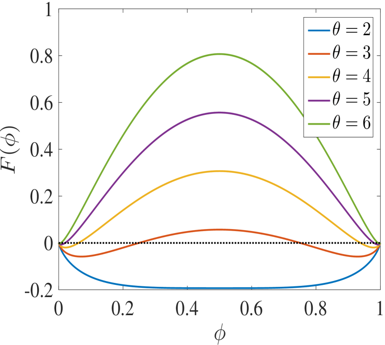
(a) Energy potential

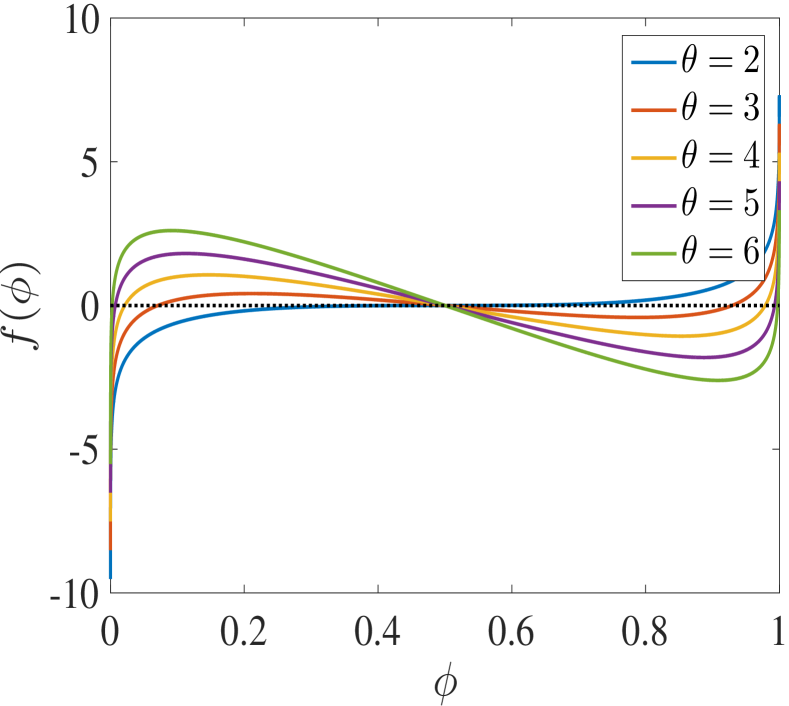
(b) Chemical potential

Fig. 1: Logarithmic Flory–Huggins energy potential and chemical potential.

3 Discrete function spaces and discrete operators

In this section, we describe the discrete function spaces, discrete operators and discrete variational principle [48, 18, 22, 25, 51, 50, 9, 31, 30], which are based on the cell-centered finite difference (CCFD) method [48, 2]. Here, we consider the two-dimensional case only, but the forms of the three-dimensional case are similar. Let $\Omega=[l_{x}^{a},l_{x}^{b}]\times[l_{y}^{a},l_{y}^{b}]$, where $l_{x}^{a}<l_{x}^{b}$ and $l_{y}^{a}<l_{y}^{b}$. For simplicity, the uniform division is used and the mesh size is denoted by $h=\frac{l_{x}^{b}-l_{x}^{a}}{N}=\frac{l_{y}^{b}-l_{y}^{a}}{M}$, where $N$ and $M$ are positive integers. The grid points are denoted by $x_{i}=l_{x}^{a}+ih$ and $y_{j}=l_{y}^{a}+jh$, and furthermore, the intermediate points are denoted by $x_{i+\frac{1}{2}}=x_{i}+\frac{1}{2}h$ and $y_{j+\frac{1}{2}}=y_{j}+\frac{1}{2}h$.

The discrete function spaces are defined as follows

$$\mathcal{C}_{h}=\big{\{}\phi:(x_{i+\frac{1}{2}},y_{j+\frac{1}{2}})\mapsto\mathbb{R},~{}~{}0\leq i\leq N-1,~{}0\leq j\leq M-1\big{\}},$$

$$\mathcal{U}_{h}=\big{\{}u:(x_{i},y_{j+\frac{1}{2}})\mapsto\mathbb{R},~{}~{}0\leq i\leq N,~{}0\leq j\leq M-1\big{\}},$$

$$\mathcal{V}_{h}=\big{\{}v:(x_{i+\frac{1}{2}},y_{j})\mapsto\mathbb{R},~{}~{}0\leq i\leq N-1,~{}0\leq j\leq M\big{\}}.$$

Here, we use the identification $\phi_{i+\frac{1}{2},j+\frac{1}{2}}=\phi(x_{i+\frac{1}{2}},y_{j+\frac{1}{2}})$, etc. The homogeneous Neumann boundary condition is considered in this paper, and the case with the homogeneous Dirichlet or periodic boundary condition can be formulated and analyzed analogously. We introduce the subsets of $\mathcal{V}_{u}$ and $\mathcal{V}_{v}$ involving the homogeneous Neumann boundary condition as

$$\mathcal{U}^{0}_{h}=\big{\{}u\in\mathcal{U}_{h}|~{}u_{0,j+\frac{1}{2}}=u_{N,j+\frac{1}{2}}=0,~{}~{}0\leq j\leq M-1\big{\}},$$ (3.1)

$$\mathcal{V}^{0}_{h}=\big{\{}v\in\mathcal{V}_{h}|~{}v_{i+\frac{1}{2},0}=v_{i+\frac{1}{2},M}=0,~{}~{}0\leq i\leq N-1\big{\}}.$$ (3.2)

For $\phi\in\mathcal{C}_{h}$, the discrete gradient operator is defined as $\nabla_{h}=[\nabla_{h,x},\nabla_{h,y}]^{T}$, where $\nabla_{h,x}\phi\in\mathcal{U}_{h}^{0}$ and $\nabla_{h,y}\phi\in\mathcal{V}_{h}^{0}$ are defined as follows

$$\nabla_{h,x}\phi_{i,j+\frac{1}{2}}=\frac{\phi_{i+\frac{1}{2},j+\frac{1}{2}}-\phi_{i-\frac{1}{2},j+\frac{1}{2}}}{h},~{}~{}1\leq i\leq N-1,~{}0\leq j\leq M-1,$$ (3.3a)

$$\nabla_{h,y}\phi_{i+\frac{1}{2},j}=\frac{\phi_{i+\frac{1}{2},j+\frac{1}{2}}-\phi_{i+\frac{1}{2},j-\frac{1}{2}}}{h},~{}~{}0\leq i\leq N-1,~{}1\leq j\leq M-1.$$ (3.3b)

For $u\in\mathcal{U}_{h}$ and $v\in\mathcal{V}_{h}$, the discrete divergence operator is defined as $\nabla_{h}\cdot[u,v]^{T}=D_{x}u+D_{y}v$, where $D_{x}$ and $D_{y}$ are defined as follows

$$D_{x}u_{i+\frac{1}{2},j+\frac{1}{2}}=\frac{u_{i+1,j+\frac{1}{2}}-u_{i,j+\frac{1}{2}}}{h},~{}~{}~{}D_{y}v_{i+\frac{1}{2},j+\frac{1}{2}}=\frac{v_{i+\frac{1}{2},j+1}-v_{i+\frac{1}{2},j}}{h},$$ (3.4)

where $0\leq i\leq N-1,~{}0\leq j\leq M-1$. The discrete Laplace operator is defined as $\Delta_{h}=\nabla_{h}\cdot\nabla_{h}$.

We define the following discrete inner-products:

$$\left(\phi,\phi^{\prime}\right)_{h}=h^{2}\sum_{i=0}^{N-1}\sum_{j=0}^{M-1}\phi_{i+\frac{1}{2},j+\frac{1}{2}}\phi^{\prime}_{i+\frac{1}{2},j+\frac{1}{2}},~{}~{}~{}\phi,\phi^{\prime}\in\mathcal{C}_{h},$$

$$\left(u,u^{\prime}\right)_{h}=h^{2}\sum_{i=1}^{N-1}\sum_{j=0}^{M-1}u_{i,j+\frac{1}{2}}u^{\prime}_{i,j+\frac{1}{2}},~{}~{}~{}u,u^{\prime}\in\mathcal{U}_{h}^{0},$$

$$\left(v,v^{\prime}\right)_{h}=h^{2}\sum_{i=0}^{N-1}\sum_{j=1}^{M-1}v_{i+\frac{1}{2},j}v^{\prime}_{i+\frac{1}{2},j},~{}~{}~{}v,v^{\prime}\in\mathcal{V}_{h}^{0}.$$

The discrete norms for $\phi\in\mathcal{C}_{h}$, $u\in\mathcal{U}_{h}^{0}$ and $v\in\mathcal{V}_{h}^{0}$ are denoted as

$$\|\phi\|_{h}=\left(\phi,\phi\right)_{h}^{1/2},~{}~{}\|u\|_{h}=\left(u,u\right)_{h}^{1/2},~{}~{}\|v\|_{h}=\left(v,v\right)_{h}^{1/2},$$

$$\|\nabla_{h}\phi\|_{h}^{2}=\|\nabla_{h,x}\phi\|_{h}^{2}+\|\nabla_{h,y}\phi\|_{h}^{2}.$$

The following discrete variational formulas are obtained by direct calculations [51, 50, 9, 31, 30]

$$\left(u,\nabla_{h,x}\phi\right)_{h}=-\left(D_{x}u,\phi\right)_{h},~{}~{}u\in\mathcal{U}_{h}^{0},~{}\phi\in\mathcal{C}_{h},$$ (3.5)

$$\left(v,\nabla_{h,y}\phi\right)_{h}=-\left(D_{y}v,\phi\right)_{h},~{}~{}v\in\mathcal{V}_{h}^{0},~{}\phi\in\mathcal{C}_{h},$$ (3.6)

$$-\left(\Delta_{h}\phi,\varphi\right)_{h}=\left(\nabla_{h}\phi,\nabla_{h}\varphi\right)_{h},~{}~{}\phi,\varphi\in\mathcal{C}_{h}.$$ (3.7)

The following lemma is a direct consequence of Lemma 5.1 in [31].

Lemma 3.1.

Let $\phi_{-}=\min(\phi-a,0)$ and $\phi_{+}=\max(\phi-b,0)$, where $\phi\in\mathcal{C}_{h}$ and $a<b$. Then we have

$$\|\nabla_{h}\phi_{-}\|_{h}^{2}\leq-\left(\Delta_{h}\phi,\phi_{-}\right)_{h},$$ (3.8)

$$\|\nabla_{h}\phi_{+}\|_{h}^{2}\leq-\left(\Delta_{h}\phi,\phi_{+}\right)_{h}.$$ (3.9)

We note that for the homogeneous Dirichlet and periodic boundary conditions, we have the similar results to (3.8) and (3.9).

4 Stabilized energy factorization approach and discrete scheme

Let $\phi^{n}$ denote the discrete function at the time level $t=t_{n}$, where $n\geq 0$. The key idea of the energy factorization (EF) approach is that we first factorize the energy function as follows

$$E(\phi)=\int_{\Omega}\sum_{i=1}^{M}\Phi_{i}(\phi)\cdot\Psi_{i}(\phi)d{\bf x},$$ (4.1)

where $\Phi_{i}(\phi)$ and $\Psi_{i}(\phi)$ are the energy factors, $M\geq 1$, and then we derive the following energy inequality using the properties of the factors

$$E(\phi^{n+1})-E(\phi^{n})\leq\int_{\Omega}\mu\left(\phi^{n+1},\phi^{n},\cdots,\phi^{0})\\ (\phi^{n+1}-\phi^{n}\right)d{\bf x}.$$ (4.2)

Thus, $\mu$ is the discrete general chemical potential, which is usually a functional of $\phi^{n+1}$ and $\phi^{n}$, and more generally may rely on $\phi^{n-1},\cdots,\phi^{0}$ as well. For a specific energy $E(\phi)$, there may be several different factorization forms, but not all of the resultant discrete chemical potentials $\mu$ are linear with respect to $\phi^{n+1}$. So an ingenious factorization approach is required for the sake of obtaining a linear efficient scheme.

As a simple example, we consider the gradient free energy

$$E_{\nabla}(\phi)=\frac{1}{2}\int_{\Omega}\epsilon^{2}|\nabla\phi|^{2}d{\bf x},$$ (4.3)

and we can derive that

$$E_{\nabla}(\phi^{n+1})-E_{\nabla}(\phi^{n}) =\frac{1}{2}\int_{\Omega}\epsilon^{2}\left(|\nabla\phi^{n+1}|^{2}-|\nabla\phi^{n}|^{2}\right)d{\bf x}$$

$$=\int_{\Omega}\epsilon^{2}\nabla\phi^{n+1}\cdot\nabla\left(\phi^{n+1}-\phi^{n}\right)d{\bf x}-\frac{1}{2}\int_{\Omega}\epsilon^{2}|\nabla(\phi^{n+1}-\phi^{n})|^{2}d{\bf x}$$

$$\leq\int_{\Omega}\epsilon^{2}\nabla\phi^{n+1}\cdot\nabla\left(\phi^{n+1}-\phi^{n}\right)d{\bf x}$$

$$=-\int_{\Omega}\left(\phi^{n+1}-\phi^{n}\right)\epsilon^{2}\Delta\phi^{n+1}d{\bf x},$$ (4.4)

which leads to the classical implicit chemical potential $\mu_{\nabla}^{n+1}=-\epsilon^{2}\Delta\phi^{n+1}$. The other treatment for $E_{\nabla}(\phi)$ is described as follows

$$E_{\nabla}(\phi^{n+1})-E_{\nabla}(\phi^{n}) =\frac{1}{2}\int_{\Omega}\epsilon^{2}\nabla\left(\phi^{n+1}+\phi^{n}\right)\cdot\nabla\left(\phi^{n+1}-\phi^{n}\right)d{\bf x}$$

$$=-\frac{1}{2}\int_{\Omega}\left(\phi^{n+1}-\phi^{n}\right)\epsilon^{2}\Delta\left(\phi^{n+1}+\phi^{n}\right)d{\bf x},$$ (4.5)

which yields the classical semi-implicit chemical potential $\mu_{\nabla}^{n+1}=-\frac{1}{2}\epsilon^{2}\Delta\left(\phi^{n+1}+\phi^{n}\right)$.

4.1 Stabilized energy factorization approach for Flory–Huggins potential

In order to treat the logarithmic Flory–Huggins potential, we introduce a stabilized energy factorization approach, which combines the stability technique with the energy factorization approach proposed in [31] for the PR-EOS based free energy. To apply the energy factorization approach, we define

$$H_{a}(\phi)=\phi\ln\left(\phi\right),~{}~{}H_{b}(\phi)=\left(1-\phi\right)\ln\left(1-\phi\right),~{}~{}H_{c}(\phi)=\theta\phi\left(1-\phi\right),$$ (4.6)

and from this, we rewrite $F(\phi)$ as

$$F(\phi)=\left(\lambda+1\right)\left(H_{a}(\phi)+H_{b}(\phi)\right)+H_{c}(\phi)-\lambda\left(H_{a}(\phi)+H_{b}(\phi)\right),$$ (4.7)

where $\lambda\geq 0$ is a constant. The stability term is crucial to ensure the symmetric positive definiteness and discrete maximum principle of the resultant scheme in the case with a large $\theta$, which will be demonstrated in Subsection 5.1 and Subsection 5.2 respectively.

It is clearly observed that $H_{a}(\phi)$ as well as $H_{b}(\phi)$ can be factorized into the product of a linear function and a logarithm function, while $H_{c}(\phi)$ is a product of two linear functions. For $\phi^{n}>0$ and $\phi^{n+1}>0$, we can deduce that

$$H_{a}(\phi^{n+1})-H_{a}(\phi^{n}) = \phi^{n+1}\ln\left(\phi^{n+1})-\phi^{n}\ln(\phi^{n}\right)$$ (4.8)

$$= \left(\phi^{n+1}-\phi^{n}\right)\ln(\phi^{n})+\phi^{n+1}\left(\ln(\phi^{n+1})-\ln(\phi^{n})\right)$$

$$\leq \left(\ln\left(\phi^{n}\right)+\frac{\phi^{n+1}}{\phi^{n}}\right)\left(\phi^{n+1}-\phi^{n}\right),$$

where the last inequality is obtained using the concavity of $\ln(\phi)$ as

$$\ln(\phi^{n+1})\leq\ln(\phi^{n})+\frac{1}{\phi^{n}}\left(\phi^{n+1}-\phi^{n}\right).$$

Noting that $\ln(1-\phi)$ is also concave, we have

$$\ln(1-\phi^{n+1})\leq\ln(1-\phi^{n})+\frac{1}{\phi^{n}-1}\left(\phi^{n+1}-\phi^{n}\right).$$

Thus, for $\phi^{n}<1$ and $\phi^{n+1}<1$, we deduce that

$$H_{b}(\phi^{n+1})-H_{b}(\phi^{n}) = \left(1-\phi^{n+1}\right)\ln\left(1-\phi^{n+1})-\left(1-\phi^{n}\right)\ln(1-\phi^{n}\right)$$ (4.9)

$$= -\left(\phi^{n+1}-\phi^{n}\right)\ln(1-\phi^{n})$$

$$+\left(1-\phi^{n+1}\right)\left(\ln(1-\phi^{n+1})-\ln(1-\phi^{n})\right)$$

$$\leq \left(-\ln(1-\phi^{n})+\frac{1-\phi^{n+1}}{\phi^{n}-1}\right)\left(\phi^{n+1}-\phi^{n}\right).$$

For $H_{c}(\phi)$, we apply the factorization approach to deal with $H_{c}(\phi)$ as follows

$$H_{c}(\phi^{n+1})-H_{c}(\phi^{n})=\theta\left(1-\phi^{n+1}-\phi^{n}\right)\left(\phi^{n+1}-\phi^{n}\right).$$ (4.10)

Due to the concavity of $H_{a}(\phi)$, we have $\ln(\phi^{n})-\ln(\phi^{n+1})\leq\frac{1}{\phi^{n+1}}\left(\phi^{n}-\phi^{n+1}\right)$, thus we deduce

$$H_{a}(\phi^{n})-H_{a}(\phi^{n+1}) = \phi^{n}\ln\left(\phi^{n}\right)-\phi^{n+1}\ln\left(\phi^{n+1}\right)$$ (4.11)

$$= \left(\phi^{n}-\phi^{n+1}\right)\ln(\phi^{n})+\phi^{n+1}\left(\ln(\phi^{n})-\ln(\phi^{n+1})\right)$$

$$\leq -\left(\ln\left(\phi^{n}\right)+1\right)\left(\phi^{n+1}-\phi^{n}\right).$$

It is similar to deduce that

$$H_{b}(\phi^{n})-H_{b}(\phi^{n+1})\leq\left(\ln\left(1-\phi^{n}\right)+1\right)\left(\phi^{n+1}-\phi^{n}\right).$$ (4.12)

Using (4.8)-(4.12), we define the discrete chemical potential as

$$f(\phi^{n},\phi^{n+1}) = \left(\lambda+1\right)\left(\ln\left(\phi^{n}\right)+\frac{\phi^{n+1}}{\phi^{n}}-\ln(1-\phi^{n})-\frac{1-\phi^{n+1}}{1-\phi^{n}}\right)$$ (4.13)

$$+\theta\left(1-\phi^{n+1}-\phi^{n}\right)-\lambda\left(\ln\left(\phi^{n}\right)+1\right)+\lambda\left(\ln\left(1-\phi^{n}\right)+1\right)$$

$$= \ln\left(\phi^{n}\right)-\ln(1-\phi^{n})+\left(\lambda+1\right)\left(\frac{\phi^{n+1}}{\phi^{n}}-\frac{1-\phi^{n+1}}{1-\phi^{n}}\right)$$

$$+\theta\left(1-\phi^{n+1}-\phi^{n}\right).$$

From (4.7)-(4.13), we obtain the following energy inequality

$$F(\phi^{n+1})-F(\phi^{n})\leq f(\phi^{n},\phi^{n+1})\left(\phi^{n+1}-\phi^{n}\right).$$ (4.14)

There is the other alternative approach for $H_{c}(\phi)$ on the basis of the concavity of $H_{c}(\phi)$, which is expressed as

$$H_{c}(\phi^{n+1})-H_{c}(\phi^{n})\leq\theta\left(1-2\phi^{n}\right)\left(\phi^{n+1}-\phi^{n}\right).$$ (4.15)

In this case, the chemical potential $f(\phi^{n},\phi^{n+1})$ is defined as below

$$f(\phi^{n},\phi^{n+1}) = \ln\left(\phi^{n}\right)-\ln(1-\phi^{n})+\left(\lambda+1\right)\left(\frac{\phi^{n+1}}{\phi^{n}}-\frac{1-\phi^{n+1}}{1-\phi^{n}}\right)$$ (4.16)

$$+\theta\left(1-2\phi^{n}\right).$$

It is observed from numerical tests that the treatment given in (4.10) performs better than that of (4.15).

4.2 Fully discrete scheme

The semi-implicit discrete scheme for the Allen-Cahn equation with the logarithmic Flory–Huggins potential is stated as: given $\phi^{n}\in\mathcal{C}_{h}$, find $\phi^{n+1}\in\mathcal{C}_{h}$ such that

$$\frac{\phi^{n+1}-\phi^{n}}{\tau}-\epsilon^{2}\Delta_{h}\phi^{n+1}+f(\phi^{n},\phi^{n+1})=0,$$ (4.17)

where $\tau$ denotes the time step size, $f(\phi^{n},\phi^{n+1})$ is defined in (4.13) or (4.16) and $\phi^{0}$ is provided by the initial condition.

In what follows, we will consider only $f(\phi^{n},\phi^{n+1})$ defined in (4.13) in theoretical analysis, but the scheme with (4.16) can be analyzed in a very similar routine.

For convenience of theoretical analysis, using (4.13), we rewrite (4.17) as the following equivalent from

$$\frac{1}{\tau}\left(\phi^{n+1}-\phi^{n}\right)-\epsilon^{2}\Delta_{h}\phi^{n+1}+\nu_{\theta,\lambda}(\phi^{n})\phi^{n+1}=r_{\theta,\lambda}(\phi^{n}),$$ (4.18)

where $\nu_{\theta,\lambda}(\phi)$ and $r_{\theta,\lambda}(\phi)$ are defined as follows

$$\nu_{\theta,\lambda}(\phi)=\left(\lambda+1\right)\left(\frac{1}{\phi}+\frac{1}{1-\phi}\right)-\theta,$$ (4.19)

$$r_{\theta,\lambda}(\phi) =-\ln\left(\phi\right)+\ln(1-\phi)+\frac{\lambda+1}{1-\phi}-\theta\left(1-\phi\right).$$ (4.20)

Remark 4.1.

Since the linear discrete chemical potentials are obtained using the energy factorization approach, the proposed discrete scheme is linear, easy to implement, and preserve the original energy dissipation law. However, the commonly used convex splitting approach for the logarithmic Flory–Huggins potential results in the nonlinear discrete chemical potential as well as the nonlinear schemes [8].

5 Theoretical analysis

In this section, we will prove the well-posedness and maximum principle of the discrete solution. In particular, we will demonstrate that $\lambda$ is essential to ensure the maximum principle. The unconditional energy stability of the proposed scheme will be proved as well.

5.1 Existence and uniqueness

For given $\phi^{n}$, we define the linear operator as follows

$${\bf Q}^{n}_{\theta,\lambda}=-\epsilon^{2}\Delta_{h}+\nu_{\theta,\lambda}(\phi^{n}).$$ (5.1)

Lemma 5.1.

Assume that $0<\phi^{n}<1$. For given $\theta>2$, if $\lambda$ is chosen such that

$$\lambda\geq 0~{}~{}\textnormal{and}~{}~{}\lambda>\frac{1}{4}\theta-1,$$ (5.2)

then ${\bf Q}^{n}_{\theta,\lambda}$ is symmetric and positive definite.

Proof.

${\bf Q}^{n}_{\theta,\lambda}$ is symmetric since for $\phi,\varphi\in\mathcal{C}_{h}$, we have

$$\left({\bf Q}^{n}_{\theta,\lambda}\phi,\varphi\right)_{h} =-\epsilon^{2}\left(\Delta_{h}\phi,\varphi\right)_{h}+\left(\nu_{\theta,\lambda}(\phi^{n})\phi,\varphi\right)_{h}$$

$$=\epsilon^{2}\left(\nabla_{h}\phi,\nabla_{h}\varphi\right)_{h}+\left(\nu_{\theta,\lambda}(\phi^{n})\phi,\varphi\right)_{h}$$

$$=-\epsilon^{2}\left(\Delta_{h}\varphi,\phi\right)_{h}+\left(\nu_{\theta,\lambda}(\phi^{n})\varphi,\phi\right)_{h}=\left({\bf Q}^{n}_{\theta,\lambda}\varphi,\phi\right)_{h}.$$ (5.3)

We now prove that ${\bf Q}^{n}_{\theta,\lambda}$ is positive definite. Let $\xi(s)=\frac{1}{s}+\frac{1}{1-s}$ for a scalar number $0<s<1$, then the derivative of $\xi(s)$ is expressed as

$$\xi(s)=-\frac{1}{s^{2}}+\frac{1}{(1-s)^{2}}.$$

We observe that $\xi^{\prime}(s)\leq 0$ for $s\in(0,\frac{1}{2}]$ and $\xi^{\prime}(s)\geq 0$ for $s\in[\frac{1}{2},1)$, thus

$$\nu_{\theta,\lambda}(s)\geq 4\left(\lambda+1\right)-\theta>0.$$ (5.4)

For $\phi\in\mathcal{C}_{h}$ and $\phi\neq 0$, we deduce that

$$\left({\bf Q}^{n}_{\theta,\lambda}\phi,\phi\right)_{h} =\epsilon^{2}\left(\nabla_{h}\phi,\nabla_{h}\phi\right)_{h}+\left(\nu_{\theta,\lambda}(\phi^{n})\phi,\phi\right)_{h}$$

$$\geq\epsilon^{2}\|\nabla_{h}\phi\|^{2}_{h}+\left(4\left(\lambda+1\right)-\theta\right)\|\phi\|_{h}^{2}>0,$$ (5.5)

which yields the positive definiteness of ${\bf Q}^{n}_{\theta,\lambda}$. ∎

Remark 5.1.

For $2<\theta<4$, the condition (5.2) holds if $\lambda=0$. But for $\theta\geq 4$, a positive stability constant satisfying $\lambda>\frac{1}{4}\theta-1$ is required to ensure the positive definiteness of ${\bf Q}^{n}_{\theta,\lambda}$. We also note that the linear system of the scheme with (4.16) is symmetric and positive definite for any $\theta>2$ and $\lambda\geq 0$.

We now prove the existence and uniqueness of the discrete solution of (4.18).

Theorem 5.1.

Assume that $0<\phi^{n}<1$. For any time step size $\tau>0$, there exists a unique $\phi^{n+1}$ to solve (4.18) in $\mathcal{C}_{h}$ provided that $\lambda$ is chosen to satisfy (5.2).

Proof.

It suffices to prove that the following homogeneous equation has a unique zero solution in $\mathcal{C}_{h}$

$$\frac{1}{\tau}\phi-\epsilon^{2}\Delta_{h}\phi+\nu_{\theta,\lambda}(\phi^{n})\phi=0,$$ (5.6)

which can be rewritten as

$$\frac{1}{\tau}\phi+{\bf Q}^{n}_{\theta,\lambda}\phi=0.$$ (5.7)

As a direct consequence of the symmetric positive definiteness of ${\bf Q}^{n}_{\theta,\lambda}$, there is a unique solution $\phi\equiv 0$. ∎

5.2 Discrete maximum principle

The maximum principle of the discrete solution essentially relies on the stability constant for given energy parameter $\theta$, thus we need to employ the proper stability constant $\lambda$ to ensure this key property. We denote

$$L(\theta,\lambda)=\min_{0<\phi<1}r_{\theta,\lambda}(\phi),$$ (5.8)

$$U(\theta,\lambda)=\max_{0<\phi<1}\big{(}r_{\theta,\lambda}(\phi)-\nu_{\theta,\lambda}(\phi)\big{)}.$$ (5.9)

In order to ensure the maximum principle of the proposed scheme, we introduce the following condition: for given $\theta>2$, $\lambda$ shall be taken to satisfy (5.2) and

$$L(\theta,\lambda)>0,~{}~{}U(\theta,\lambda)<0.$$ (5.10)

Remark 5.2.

We illustrate the reasonability of the condition (5.10) in Figure 2. Here, the values of $\lambda$ are taken as follows

$$\lambda=\left\{\begin{array}[]{ccc}0,&2<\theta\leq 3,\\ 1,&3<\theta\leq 4.5,\\ 2,&4.5<\theta\leq 6.\end{array}\right.$$ (5.11)

It can be observed from Figure 2 that the condition (5.10) naturally holds for $2<\theta\leq 3$ without any stability term, while it is still true for $3<\theta\leq 6$ when we take the small values (1 and 2) for the stability constant $\lambda$ as in (5.11). We have also checked some cases of $\theta>6$ and found that the condition (5.10) is true if $\lambda$ is properly chosen. We also emphasize that (5.10) is a good guide to choose $\lambda$ since it is clearly independent of discrete solutions. For the scheme with (4.16), we have the similar condition for the choice of the stability constant.

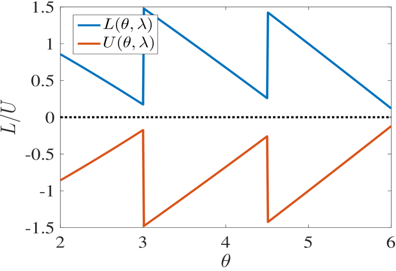
Fig. 2: Verification of the condition (5.10).

The following theorem demonstrates that the scheme (4.18) with the appropriate stability constant preserves the discrete maximum principle.

Theorem 5.2.

Assume that $0<\phi^{0}<1,$ and $\lambda$ is chosen to satisfy (5.2) and (5.10) for given $\theta>2$. For any time step size, the solutions of the scheme (4.18) satisfy $0<\phi^{n}<1$, $n\geq 1$.

Proof.

By induction, assuming $0<\phi^{n}<1$, we prove $0<\phi^{n+1}<1$. There exists a unique $\phi^{n+1}\in\mathcal{C}_{h}$ in terms of Theorem 5.1. Let us define $\phi_{-}^{n+1}=\min(\phi^{n+1},0)$. It is obtained from (4.18) that

$$\frac{1}{\tau}\left(\phi^{n+1}-\phi^{n},\phi_{-}^{n+1}\right)_{h}-\epsilon^{2}\left(\Delta_{h}\phi^{n+1},\phi_{-}^{n+1}\right)_{h}+\left(\nu_{\theta,\lambda}(\phi^{n})\phi^{n+1},\phi_{-}^{n+1}\right)_{h}$$

$$~{}~{}~{}=\left(r_{\theta,\lambda}(\phi^{n}),\phi_{-}^{n+1}\right)_{h}.$$ (5.12)

The definition of $\phi_{-}^{n+1}$ yields

$$\left(\phi^{n+1},\phi_{-}^{n+1}\right)_{h}=\|\phi_{-}^{n+1}\|_{h}^{2}.$$ (5.13)

Moreover, it is apparent that $\phi_{-}^{n+1}\leq 0$. Due to $\phi^{n}>0$, we have

$$\left(\phi^{n},\phi_{-}^{n+1}\right)_{h}\leq 0.$$ (5.14)

Thus the first term on the left-hand side of (5.2) is bounded as

$$\left(\phi^{n+1}-\phi^{n},\phi_{-}^{n+1}\right)_{h}=\|\phi_{-}^{n+1}\|_{h}^{2}-\left(\phi^{n},\phi_{-}^{n+1}\right)_{h}\geq\|\phi_{-}^{n+1}\|_{h}^{2}.$$ (5.15)

Applying (3.8), the second term on the left-hand side of (5.2) is bounded as

$$-\epsilon^{2}\left(\Delta_{h}\phi^{n+1},\phi_{-}^{n+1}\right)_{h}\geq\epsilon^{2}\|\nabla_{h}\phi_{-}^{n+1}\|_{h}^{2}.$$ (5.16)

The third term on the left-hand side of (5.2) is bounded below

$$\left(\nu_{\theta,\lambda}(\phi^{n})\phi^{n+1},\phi_{-}^{n+1}\right)_{h}\geq\left(4\left(\lambda+1\right)-\theta\right)\|\phi_{-}^{n+1}\|_{h}^{2}.$$ (5.17)

Using the condition (5.10) and taking into account $\phi_{-}^{n+1}\leq 0$, the right-hand side of (5.2) is estimated as

$$\left(r_{\theta,\lambda}(\phi^{n}),\phi_{-}^{n+1}\right)_{h}\leq\left(L(\theta,\lambda),\phi_{-}^{n+1}\right)_{h}\leq 0.$$ (5.18)

We combine (5.13)-(5.18) and obtain

$$\frac{1}{\tau}\|\phi_{-}^{n+1}\|_{h}^{2}+\epsilon^{2}\|\nabla_{h}\phi_{-}^{n+1}\|_{h}^{2}+\left(4\left(\lambda+1\right)-\theta\right)\|\phi_{-}^{n+1}\|_{h}^{2}\leq 0.$$ (5.19)

It follows from (5.19) that $\|\phi_{-}^{n+1}\|_{h}^{2}=0$ and consequently, we get $\phi^{n+1}\geq 0$. We further prove that $\phi^{n+1}>0$ by contradiction. Suppose that there exists at least a grid point $(i_{0}+\frac{1}{2},j_{0}+\frac{1}{2})$ such that $\phi^{n+1}_{i_{0}+\frac{1}{2},j_{0}+\frac{1}{2}}=0$, then the equation (4.18) at $(i_{0}+\frac{1}{2},j_{0}+\frac{1}{2})$ has the form

$$-\frac{1}{\tau}\phi^{n}_{i_{0}+\frac{1}{2},j_{0}+\frac{1}{2}}-\epsilon^{2}\Delta_{h}\phi_{i_{0}+\frac{1}{2},j_{0}+\frac{1}{2}}^{n+1}=r_{\theta,\lambda}\big{(}\phi^{n}_{i_{0}+\frac{1}{2},j_{0}+\frac{1}{2}}\big{)}.$$ (5.20)

The right-hand side of (5.20) can be estimated using (5.10) as

$$r_{\theta,\lambda}\big{(}\phi^{n}_{i_{0}+\frac{1}{2},j_{0}+\frac{1}{2}}\big{)}\geq L(\theta,\lambda)>0.$$ (5.21)

For the two terms on the left-hand side of (5.20), we obtain

$$-\frac{1}{\tau}\phi^{n}_{i_{0}+\frac{1}{2},j_{0}+\frac{1}{2}}-\epsilon^{2}\Delta_{h}\phi_{i_{0}+\frac{1}{2},j_{0}+\frac{1}{2}}^{n+1}<0,$$ (5.22)

which contradict (5.21). Therefore, $\phi^{n+1}>0$.

To prove $\phi^{n+1}<1$, we define $\phi_{+}^{n+1}=\max(\phi^{n+1}-1,0)$. We get from (4.18) that

$$\frac{1}{\tau}\left(\phi^{n+1}-\phi^{n},\phi_{+}^{n+1}\right)_{h}-\epsilon^{2}\left(\Delta_{h}\phi^{n+1},\phi_{+}^{n+1}\right)_{h}+\left(\nu_{\theta,\lambda}(\phi^{n})(\phi^{n+1}-1),\phi_{+}^{n+1}\right)_{h}$$

$$=\left(r_{\theta,\lambda}(\phi^{n})-\nu_{\theta,\lambda}(\phi^{n}),\phi_{+}^{n+1}\right)_{h}.$$ (5.23)

The definition of $\phi_{+}^{n+1}$ implies that

$$\phi_{+}^{n+1}\geq 0,~{}~{}\left(\phi^{n+1}-1,\phi_{+}^{n+1}\right)_{h}=\|\phi_{+}^{n+1}\|_{h}^{2}.$$ (5.24)

Taking into account $\phi^{n}<1$, we have

$$\left(\phi^{n}-1,\phi_{+}^{n+1}\right)_{h}\leq 0.$$ (5.25)

The first term of (5.2) is bounded below using (5.24) and (5.25)

$$\left(\phi^{n+1}-\phi^{n},\phi_{+}^{n+1}\right)_{h}=\|\phi_{+}^{n+1}\|_{h}^{2}-\left(\phi^{n}-1,\phi_{+}^{n+1}\right)_{h}\geq\|\phi_{+}^{n+1}\|_{h}^{2}.$$ (5.26)

Similar to (5.16) and (5.17), we have

$$-\epsilon^{2}\left(\Delta_{h}\phi^{n+1},\phi_{+}^{n+1}\right)_{h}\geq\epsilon^{2}\|\nabla_{h}\phi_{+}^{n+1}\|_{h}^{2},$$ (5.27)

$$\left(\nu_{\theta,\lambda}(\phi^{n})(\phi^{n+1}-1),\phi_{+}^{n+1}\right)_{h}\geq\left(4\left(\lambda+1\right)-\theta\right)\|\phi_{+}^{n+1}\|_{h}^{2},$$ (5.28)

where (5.27) results from (3.9). Applying the condition (5.10) and $\phi_{+}^{n+1}\geq 0$, we derive

$$\left(r_{\theta,\lambda}(\phi^{n})-\nu_{\theta,\lambda}(\phi^{n}),\phi_{+}^{n+1}\right)_{h}\leq\left(U(\theta,\lambda),\phi_{+}^{n+1}\right)_{h}\leq 0.$$ (5.29)

Finally, we reach

$$\frac{1}{\tau}\|\phi_{+}^{n+1}\|_{h}^{2}+\epsilon^{2}\|\nabla_{h}\phi_{+}^{n+1}\|_{h}^{2}+\left(4\left(\lambda+1\right)-\theta\right)\|\phi_{+}^{n+1}\|_{h}^{2}\leq 0,$$ (5.30)

which implies that $\|\phi_{+}^{n+1}\|_{h}^{2}=0$, and thus, $\phi^{n+1}\leq 1$. We further prove that $\phi^{n+1}\neq 1$ in any grid cell by contradiction. Suppose that $\phi^{n+1}_{i_{0}+\frac{1}{2},j_{0}+\frac{1}{2}}=1$, and then the equation (4.18) at $(i_{0}+\frac{1}{2},j_{0}+\frac{1}{2})$ becomes

$$\frac{1}{\tau}\left(1-\phi^{n}_{i_{0}+\frac{1}{2},j_{0}+\frac{1}{2}}\right)-\epsilon^{2}\Delta_{h}\phi_{i_{0}+\frac{1}{2},j_{0}+\frac{1}{2}}^{n+1}=r_{\theta,\lambda}\big{(}\phi^{n}_{i_{0}+\frac{1}{2},j_{0}+\frac{1}{2}}\big{)}-\nu_{\theta,\lambda}\big{(}\phi^{n}_{i_{0}+\frac{1}{2},j_{0}+\frac{1}{2}}\big{)}.$$ (5.31)

The right-hand side of (5.31) can be estimated using (5.10) as

$$r_{\theta,\lambda}\big{(}\phi^{n}_{i_{0}+\frac{1}{2},j_{0}+\frac{1}{2}}\big{)}-\nu_{\theta,\lambda}\big{(}\phi^{n}_{i_{0}+\frac{1}{2},j_{0}+\frac{1}{2}}\big{)}\leq U(\theta,\lambda)<0,$$ (5.32)

while the two terms on the left-hand side of (5.31) are estimated as

$$\frac{1}{\tau}\left(1-\phi^{n}_{i_{0}+\frac{1}{2},j_{0}+\frac{1}{2}}\right)>0,~{}~{}-\epsilon^{2}\Delta_{h}\phi_{i_{0}+\frac{1}{2},j_{0}+\frac{1}{2}}^{n+1}\geq 0.$$ (5.33)

Substituting (5.32) and (5.33) into (5.31) yields a contradiction, and consequently, we obtain $\phi^{n+1}<1$. ∎

5.3 Unconditional energy stability

For $\phi\in\mathcal{C}_{h}$, the discrete total free energy is defined as

$$E_{h}(\phi)=\left(F(\phi),1\right)_{h}+\frac{1}{2}\epsilon^{2}\|\nabla_{h}\phi\|_{h}^{2}.$$ (5.34)

Theorem 5.3.

Assume that $0<\phi^{0}<1$ and $\lambda$ is chosen to satisfy (5.2) and (5.10) for given $\theta>2$. For any time step size $\tau$, the total free energy of the scheme (4.18) is dissipated with time steps, i.e.,

$$E_{h}(\phi^{n+1})\leq E_{h}(\phi^{n}).$$ (5.35)

Proof.

Theorems 5.1 and 5.2 argue that there exists a unique $\phi^{n}\in\mathcal{C}_{h}$ and $0<\phi^{n}<1$ for $n\geq 1$. The inequality (4.14) yields

$$\left(F(\phi^{n+1})-F(\phi^{n}),1\right)_{h}\leq\left(f(\phi^{n},\phi^{n+1}),\phi^{n+1}-\phi^{n}\right)_{h}.$$ (5.36)

On the other hand, using (3.7), we can derive that

$$\frac{1}{2}\left(\|\nabla_{h}\phi^{n+1}\|_{h}^{2}-\|\nabla_{h}\phi^{n}\|_{h}^{2}\right) =\left(\nabla_{h}\phi^{n+1},\nabla_{h}\left(\phi^{n+1}-\phi^{n}\right)\right)_{h}-\frac{1}{2}\left\|\nabla_{h}\left(\phi^{n+1}-\phi^{n}\right)\right\|_{h}^{2}$$

$$\leq\left(\nabla_{h}\phi^{n+1},\nabla_{h}\left(\phi^{n+1}-\phi^{n}\right)\right)_{h}$$

$$=-\left(\Delta_{h}\phi^{n+1},\phi^{n+1}-\phi^{n}\right)_{h}.$$ (5.37)

Using (4.17), (5.36) and (5.3), we deduce

$$E_{h}(\phi^{n+1})-E_{h}(\phi^{n}) \leq\left(-\epsilon^{2}\Delta_{h}\phi^{n+1}+f(\phi^{n},\phi^{n+1}),\phi^{n+1}-\phi^{n}\right)_{h}$$

$$\leq-\frac{1}{\tau}\|\phi^{n+1}-\phi^{n}\|_{h}^{2},$$ (5.38)

which yields (5.35). ∎

Remark 5.3.

We note that (5.10) is just a sufficient condition to ensure the discrete maximum principle. The energy dissipation law always holds as long as $0<\phi^{n}<1$, $n\geq 1$. We apply the discrete chemical potential (4.13) for solving the Cahn–Hilliard equation and find that $\phi^{n}$ always falls in $(0,1)$, thus the energy dissipation is still validated.

6 Numerical results

In this section, we present numerical results to show the effectiveness of the proposed scheme. In all numerical experiments, the computational domain is $\Omega=[-1,1]^{2}$, which is divided using a uniform mesh with $100\times 100$ elements. Here, we take $\epsilon=0.05$. The proposed scheme admits a very time step size in theory, so we take the time step size $\tau=10^{10}$ for the purpose of verifying this feature.

In this example, we compare the discrete chemical potentials proposed in (4.13) and (4.16). We take $\theta=3$ and $\lambda=0$. The initial condition of the phase variable is given as

$$\phi(x,y)=\left\{\begin{array}[]{ccc}10^{-5},&|x|\leq 0.35~{}~{}\textnormal{and}~{}~{}|y|\leq 0.35,\\ 1-10^{-5},&\textnormal{otherwise}.\end{array}\right.$$ (6.1)

Figure 3 depicts that the maximum and minimum values of the phase variable computed by the proposed scheme with (4.13) or (4.16) at each time point. Although the initial maximum and minimum values of $\phi^{n}$ are set to approach the singular points, all of $\phi^{n}$ never go beyond $(0,1)$ in the subsequent time, and consequently the maximum principle is always preserved by both (4.13) and (4.16).

Figure 4 demonstrates that the total energies are always decreasing with time steps. The proposed scheme with (4.13) has more rapid dissipation rate than that with (4.16), thus the square-shape phase simulated by the former can be shrinking into a circle more rapidly. This phenomenon is observed in Figure 5, which illustrates the dynamical evolution process of the phase variable at different time steps. The superiority of (4.13) results from the semi-implicit treatment for $H_{c}(\phi)$, while it is treated explicitly in (4.16).

(a) the scheme with (4.13)

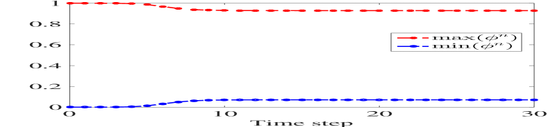
(b) the scheme with (4.16)

Fig. 3: Verification of the maximum principle.

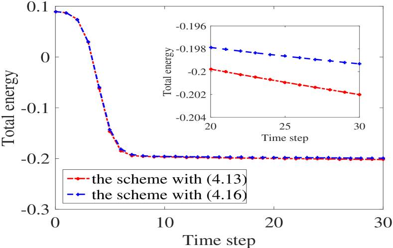
Fig. 4: Energy curves.

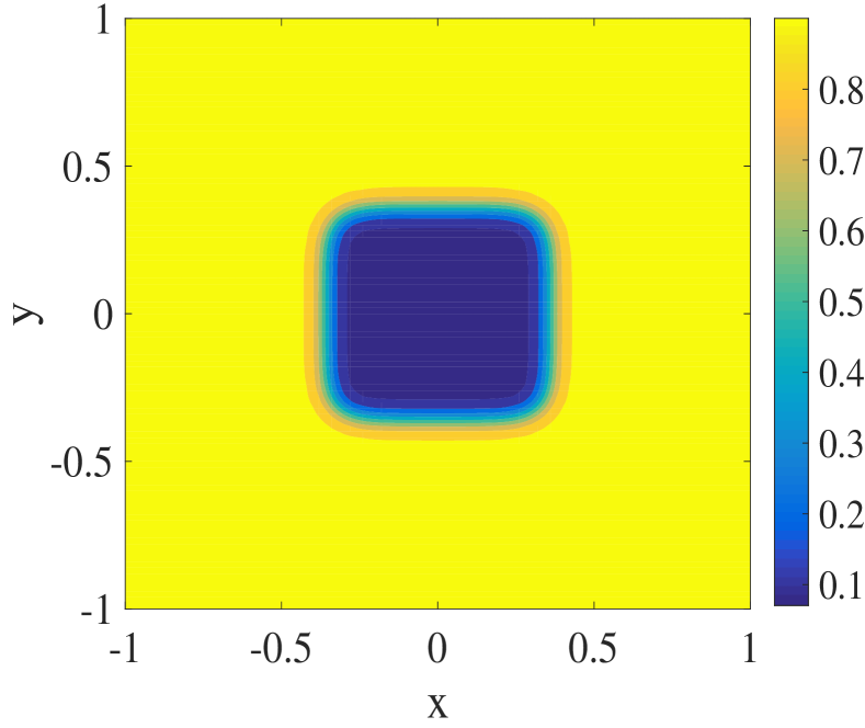
(a) scheme with (4.13), $n=10$

(b) scheme with (4.13), $n=20$

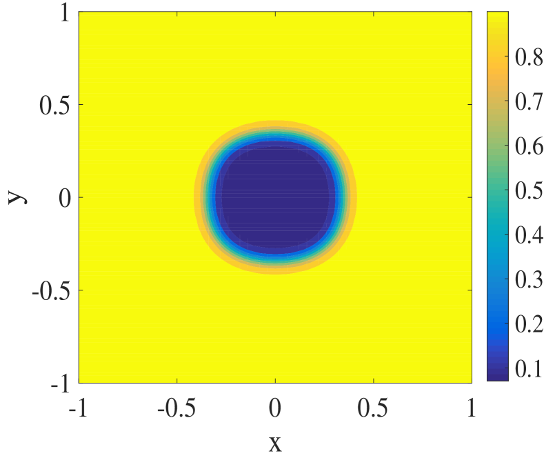
(c) scheme with (4.13), $n=30$

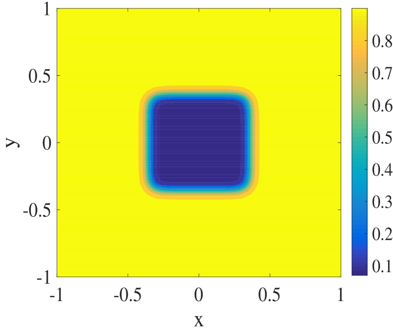
(d) scheme with (4.16), $n=10$

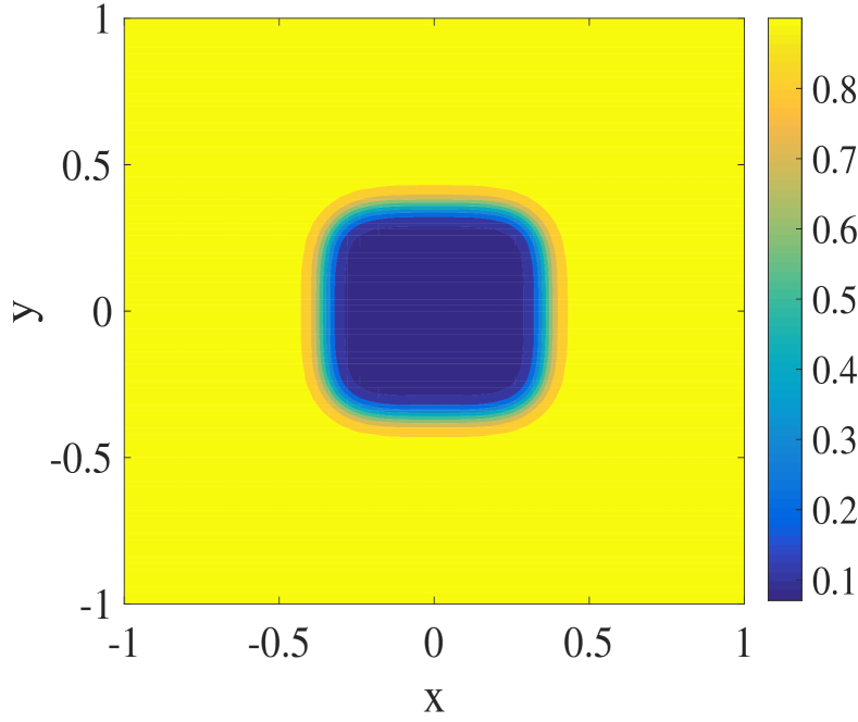
(e) scheme with (4.16), $n=20$

(f) scheme with (4.16), $n=30$

Fig. 5: The dynamical evolution of the phase variable computed by the scheme with (4.13) or (4.16) at different time steps.

7 Conclusions

The stabilized energy factorization approach has been developed to treat the logarithmic Flory–Huggins potential semi-implicitly. The stability term can eliminate the instability caused by the large energy parameter. Compared to the prevalent convex-splitting approach and auxiliary variable approaches, such approach leads to the simply linear numerical scheme inheriting the original energy dissipation law. To our best knowledge, the proposed scheme is the first such linear, unconditionally original energy stable scheme for the logarithmic Flory–Huggins potential. Moreover, the proposed scheme is rigorously proved to satisfy the discrete maximum principle under the appropriate choices of the stability constant. Numerical results are in good agreement with theoretical analysis.

In addition, the proposed scheme can be extended to the Cahn–Hilliard equation and the corresponding numerical results (not presented here) demonstrate that the maximum principle and unconditional energy stability are still validated as long as the proper stability constant is taken although theoretical proof may be not available for the maximum principle of the Cahn–Hilliard equation.

References

- [1] S.M. Allen and J.W. Cahn. A microscopic theory for antiphase boundary motion and its application to antiphase domain coarsening, Acta Metall, 27: 1085–1095, 1979.
- [2] T. Arbogast, M.F. Wheeler, I. Yotov. Mixed finite elements for elliptic problems with tensor coefficients as cell-centered finite differences. SIAM Journal on Numerical Analysis, 34(2): 828–852, 1997.
- [3] A. Baskaran, J. Lowengrub, C. Wang, S. Wise. Convergence analysis of a second order convex splitting scheme for the modified phase field crystal equation. SIAM Journal on Numerical Analysis, 51(5): 2851–2873, 2013.
- [4] F. Boyer and S. Minjeaud. Numerical schemes for a three component Cahn–Hilliard model. ESAIM: M2AN, 45:697738, 2011.
- [5] J. W. Cahn and S. M. Allen. A microscopic theory for domain wall motion and its experimental varification in fe-al alloy domain growth kinetics. J. Phys. Colloque, C7:C7–51, 1977.
- [6] J. W. Cahn and J. E. Hilliard. Free energy of a nonuniform system. I. interfacial free energy. J. Chem. Phys., 28: 258–267, 1958.
- [7] R. Chen, G. Ji, X. Yang, and H. Zhang. Decoupled energy stable schemes for phase-field vesicle membrane model. Journal of Computational Physics, 302:509–523, 2015.
- [8] W. Chen, C. Wang, X. Wang, S. M. Wise. A positivity-preserving, energy stable numerical scheme for the Cahn-Hilliard equation with logarithmic potential. arXiv, preprint, 2017.
- [9] Y. Chen, J. Shen. Efficient, adaptive energy stable schemes for the incompressible Cahn-Hilliard Navier-Stokes phase-field models. Journal of Computational Physics, 308: 40–56, 2016.
- [10] M. I. M. Copetti and C. M. Elliott. Numerical analysis of the Cahn-Hilliard equation with a logarithmic free energy. Numer. Math., 63(4): 39–65, 1992.
- [11] D. Han and X. Wang. A second order in time, uniquely solvable, unconditionally stable numerical scheme for Cahn-Hilliard-Navier-Stokes equation. Journal of Computational Physics, 290: 139–156, 2015.
- [12] C. M. Elliott, A. M. Stuart, The global dynamics of discrete semilinear parabolic equations, SIAM Journal on Numerical Analysis, 30: 1622–1663, 1993.
- [13] L.C. Evans, H.M. Soner and P.E. Souganidis. Phase transitions and generalized motion by mean curvature. Commun. Pure Appl. Math., 45: 1097–1123, 1992.
- [14] D. J. Eyre. Unconditionally gradient stable time marching the Cahn-Hilliard equation. Computational and mathematical models of microstructural evolution (San Francisco, CA, 1998), Mater. Res. Soc. Sympos. Proc., 529: 39–46. MRS, Warrendale, PA, 1998.
- [15] X. Fan, J. Kou, Z. Qiao, S. Sun. A Componentwise Convex Splitting Scheme for Diffuse Interface Models with Van der Waals and Peng-Robinson Equations of State. SIAM Journal on Scientific Computing, 39(1): B1–B28, 2017.
- [16] X. Feng and A. Prohl. Numerical analysis of the Allen-Cahn equation and approximation for mean curvature flows. Numerische Mathematik, 94(1): 33–65, 2003.
- [17] X. Feng, H. Song, T. Tang and J. Yang. Nonlinearly stable implicit-explicit methods for the Allen-Cahn equation. Inverse Problems and Image, 7: 679–695, 2013.
- [18] D. Furihata. A stable and conservative finite difference scheme for the Cahn-Hilliard equation. Numerische Mathematik, 87: 675–699, 2001.
- [19] H. Gomez and T. Hughes. Provably unconditionally stable, second-order time-accurate, mixed variational methods for phase-field models, Journal of Computational Physics, 230: 5310–5327, 2011.
- [20] H. Gomez, V.M. Calo, Y. Bazilevs, Thomas J.R. Hughes. Isogeometric analysis of the Cahn-Hilliard phase-field model. Computer Methods in Applied Mechanics and Engineering, 197: 4333–4352, 2008.
- [21] F. Guillén-González and G. Tierra. On linear schemes for a Cahn-Hilliard diffuse interface model. Journal of Computational Physics, 234: 140–171, 2013.
- [22] Z. Hu, S.M. Wise, C. Wang, J.S. Lowengrub. Stable and efficient finite-difference nonlinear-multigrid schemes for the phase field crystal equation, Journal of Computational Physics, 228: 5323–5339, 2009.
- [23] M. Kstner, P. Metsch, R. de Borst. Isogeometric analysis of the Cahn-Hilliard equation–a convergence study. Journal of Computational Physics, 305: 360–371, 2016.
- [24] D. Kay, V. Styles, E. Suli. Discontinuous Galerkin finite element approximation of the Cahn-Hilliard Equation with convection. SIAM Journal on Numerical Analysis, 47: 2660–2685, 2009.
- [25] N. Khiari, T. Achouri, M. Ben Mohamed, K. Omrani. Finite difference approximate solutions for the Cahn-Hilliard equation. Numer. Methods Partial Differ. Eqs., 23: 437–455, 2007.
- [26] J. Kim. Phase-field models for multi-component fluid flows. Commun. Comput. Phys., 12: 613–661, 2012.
- [27] J. Kou, S. Sun. Numerical methods for a multi-component two-phase interface model with geometric mean influence parameters. SIAM Journal on Scientific Computing, 37(4): B543–B569, 2015.
- [28] J. Kou, S. Sun. Efficient energy-stable dynamic modeling of compositional grading. International Journal of Numerical Analysis and Modeling, 14(2):218–242, 2017.
- [29] J. Kou, S. Sun. A stable algorithm for calculating phase equilibria with capillarity at specified moles, volume and temperature using a dynamic model. Fluid Phase Equilibria, 456: 7–24, 2018.
- [30] J. Kou, S. Sun, X. Wang. Linearly decoupled energy-stable numerical methods for multicomponent two-phase compressible flow. SIAM Journal on Numerical Analysis, 56(6): 3219–3248, 2018.
- [31] J. Kou, S. Sun, X. Wang. A novel energy factorization approach for the diffuse-interface model with Peng-Robinson equation of state. arXiv:1903.08852v1, preprint, 2019.
- [32] J. Kou, S. Sun. Thermodynamically consistent modeling and simulation of multi-component two-phase flow with partial miscibility. Computer Methods in Applied Mechanics and Engineering, 331: 623–649, 2018.
- [33] J. Kou, S. Sun. Thermodynamically consistent simulation of nonisothermal diffuse-interface two-phase flow with Peng-Robinson equation of state, Journal of Computational Physics, 371: 581–605, 2018.
- [34] J. Kou, S. Sun. Entropy stable modeling of non-isothermal multi-component diffuse-interface two-phase flows with realistic equations of state, Computer Methods in Applied Mechanics and Engineering, 341: 221–248, 2018.
- [35] H. Li, L. Ju, C. Zhang, Q. Peng. Unconditionally energy stable linear schemes for the diffuse interface model with Peng-Robinson equation of state. Journal of Scientific Computing, 75(2): 993–1015, 2018.
- [36] Y. Li, Y. Choi, J. Kim. Computationally efficient adaptive time step method for the Cahn-Hilliard equation. Computers and Mathematics with Applications, 73: 1855–1864, 2017.
- [37] C. Liu, J. Shen, and X. Yang. Decoupled energy stable schemes for a phase-field model of two-phase incompressible flows with variable density. Journal of Scientific Computing, 62: 601–622, 2015.
- [38] L. Ma, R. Chen, X. Yang, and H. Zhang. Numerical approximations for Allen-Cahn type phase field model of two-phase incompressible fluids with moving contact lines. Communications in Computational Physics, 21:867–889, 2017.
- [39] D. Peng, D.B. Robinson. A new two-constant equation of state. Industrial and Engineering Chemistry Fundamentals, 15(1): 59–64, 1976.
- [40] Q. Peng. A convex-splitting scheme for a diffuse interface model with Peng-Robinson equation of state. Advances in Applied Mathematics and Mechanics, 9(5): 1162–1188, 2017.
- [41] Z. Qiao, S. Sun. Two-phase fluid simulation using a diffuse interface model with Peng-Robinson equation of state. SIAM Journal on Scientific Computing, 36(4): B708–B728, 2014.
- [42] J. Shen, X. Yang, and H. Yu. Efficient energy stable numerical schemes for a phase field moving contact line model. Journal of Computational Physics, 284: 617–630, 2015.
- [43] J. Shen, X. Yang. Decoupled, energy stable schemes for phase-field models of two-phase incompressible flows. SIAM Journal on Numerical Analysis, 53(1): 279–296, 2015.
- [44] J. Shen, C. Wang, S. Wang, and X. Wang. Second-order convex splitting schemes for gradient flows with ehrlich-schwoebel type energy: application to thin film epitaxy. SIAM Journal on Numerical Analysis, 50: 105–125, 2012.
- [45] J. Shen, J. Xu, J. Yang. The scalar auxiliary variable (SAV) approach for gradient flows. Journal of Computational Physics, 353: 407–416, 2018.
- [46] J. Shen, J. Xu. Convergence and Error Analysis for the Scalar Auxiliary Variable (SAV) Schemes to Gradient Flows. SIAM Journal on Numerical Analysis, 56: 2895–2912, 2018.
- [47] T. Tang, J. Yang. Implicit-explicit scheme for the Allen–Cahn equation preserves the maximum principle, Journal of Computational Mathematics, 34(5): 451–461, 2016.
- [48] G. Tryggvason, R. Scardovelli, S. Zaleski. Direct Numerical Simulations of Gas-Liquid Multiphase Flows. Cambridge University Press, New York, 2011.
- [49] G.N. Wells, E. Kuhl, K. Garikipati. A discontinuous Galerkin method for the Cahn-Hilliard equation. Journal of Computational Physics, 218: 860–877, 2006.
- [50] S. M. Wise. Unconditionally Stable Finite Difference, Nonlinear Multigrid Simulation of the Cahn-Hilliard-Hele-Shaw System of Equations. Journal of Scientific Computing, 44: 38–68, 2010.
- [51] S. M. Wise, C. Wang, J. S. Lowengrub. An energy-stable and convergent finite-difference scheme for the phase field crystal equation. SIAM Journal on Numerical Analysis, 47(3): 2269–2288, 2009.
- [52] O. Wodo, B. Ganapathysubramanian. Computationally efficient solution to the Cahn–Hilliard equation: Adaptive implicit time schemes, mesh sensitivity analysis and the 3D isoperimetric problem. Journal of Computational Physics, 230: 6037–6060, 2011.
- [53] C. Xu and T. Tang. Stability analysis of large time-stepping methods for epitaxial growth models. SIAM Journal on Numerical Analysis, 44: 1759–1779, 2006.
- [54] X. Yang. Error analysis of stabilized semi-implicit method of Allen-Cahn equation. Disc. Conti. Dyn. Sys.-B, 11: 1057–1070, 2009.
- [55] X. Yang, J. Zhao. On Linear and Unconditionally Energy Stable Algorithms for Variable Mobility Cahn-Hilliard Type Equation with Logarithmic Flory-Huggins Potential. Communications in Computational Physics, 25(3): 703–728, 2019.
- [56] X. Yang, L. Ju. Efficient linear schemes with unconditionally energy stability for the phase field elastic bending energy model. Computer Methods in Applied Mechanics and Engineering, 315: 691–712, 2017.
- [57] X. Yang, J. Zhao, Q. Wang. Numerical approximations for the molecular beam epitaxial growth model based on the invariant energy quadratization method. Journal of Computational Physics, 333: 104–127, 2017.
- [58] Z. Yang, S. Dong. A Roadmap for Discretely Energy-Stable Schemes for Dissipative Systems Based on a Generalized Auxiliary Variable with Guaranteed Positivity. preprint, 2019.
- [59] S. Zhang, M. Wang. A nonconforming finite element method for the Cahn-Hilliard equation. Journal of Computational Physics, 229: 7361–7372, 2010.
- [60] J. Zhao, X. Yang, J. Shen, and Q. Wang. A decoupled energy stable scheme for a hydrodynamic phase-field model of mixtures of nematic liquid crystals and viscous fluids. Journal of Computational Physics, 305:539–556, 2016.
- [61] J. Zhao, Q. Wang, X. Yang. Numerical approximations for a phase field dendritic crystal growth model based on the invariant energy quadratization approach. Int. J. Numer. Meth. Engng, 110: 279–300, 2017.
- [62] G. Zhu, J. Kou, S. Sun, J. Yao, A. Li. Decoupled, energy stable schemes for a phase-field surfactant model. Computer Physics Communications, 233: 67–77, 2018.
- [63] G. Zhu, J. Kou, S. Sun, J. Yao, A. Li. Numerical Approximation of a Phase–Field Surfactant Model with Fluid Flow. Journal of Scientific Computing, DOI: 10.1007/s10915-019-00934-1, 2019.