Waveform systematics for binary neutron star gravitational wave signals: Effects of spin, precession, and the observation of electromagnetic counterparts

Abstract

Extracting the properties of a binary system emitting gravitational waves relies on models describing the last stages of the compact binary coalescence. In this article, we study potential biases inherent to current tidal waveform approximants for spinning and precessing systems. We perform a Bayesian study to estimate intrinsic parameters of highly spinning binary neutron star systems. Our analysis shows that one has to include the quadrupolar deformation of the neutron stars due to their rotation once dimensionless spins above $\chi\sim 0.20$ are reached, otherwise the extracted intrinsic parameters are systematically biased. We find that at design sensitivity of Advanced LIGO and Virgo, it seems unlikely that for GW170817-like sources a clear imprint of precession will be visible in the analysis of the signal employing current waveform models. However, precession effects might be detectable for unequal mass configurations with spins larger than $\chi>0.2$. We finalize our study by investigating possible benefits of a combined gravitational wave and electromagnetic detection. The presence of electromagnetic counterparts help in reducing the dimensionality of the parameter space with constraints on the sky location, source distance, and inclination. However, we note that although a small improvement in the estimation of the tidal deformability parameter is seen in these cases, changes in the intrinsic parameters are overall very small.

I Introduction

GW170817 marks a breakthrough in multi-messenger astronomy and is the first detected gravitational wave (GW) signal emerging from the coalescence of two neutron stars (NSs). This event allowed constraining the expansion rate of the universe (Abbott et al., 2017a), proved that NS mergers are the major cosmic source of r-process elements, e.g. (Eichler et al., 1989; Rosswog et al., 1999; Cowperthwaite et al., 2017; Smartt et al., 2017; Kasliwal et al., 2017; Kasen et al., 2017; Tanvir et al., 2017; Rosswog et al., 2018; Abbott et al., 2017b; Ascenzi et al., 2018), allowed a precise measurement of the speed difference between GWs and light (GBM, 2017), and placed constraints on alternative theories of gravity Ezquiaga and Zumalacárregui (2017); Baker et al. (2017); Creminelli and Vernizzi (2017). In addition, it supported the conjecture that NS mergers produce Gamma-Ray-Bursts (GRBs) (Paczynski, 1986; Eichler et al., 1989; Abbott et al., 2017c) and enabled the scientific community to investigate the supranuclear equation of state (EOS) governing the interior of NSs. These constraints arise either purely from the analysis of the GW signal, e.g., Refs. Abbott et al. (2017d); Dai et al. (2018); De et al. (2018); Abbott et al. (2018a, b, c), from a combination of GW and EM information, e.g, Refs. Radice et al. (2018); Bauswein et al. (2017); Coughlin et al. (2018a); Radice and Dai (2018); Coughlin et al. (2018b), or from a statistical analysis of a large set of possible EOSs, e.g., Annala et al. (2018); Most et al. (2018).

To extract information from the detected GW signal, one needs to cross-correlate the data with model waveforms constructed from theoretical predictions. Within the framework of Bayesian analysis, this means that a multi-dimensional likelihood function has to be computed Veitch et al. (2015). Because of the need to generate a large number of GW waveforms for evaluating the multidimensional likelihood integral numerous times, the computation of each individual waveform has to be sufficiently fast and, on the other hand, accurate enough for a precise measurement of the intrinsic source parameters.

Over the last years, there has been progress in modelling BNS coalescences by the development of improved analytical post-Newtonian (PN) based models, e.g. Damour et al. (2012); Agathos et al. (2015); Jiménez Forteza et al. (2018); Abdelsalhin et al. (2018); Pani et al. (2018), state-of-the-art tidal effective-one-body (EOB) waveform approximants, e.g., Bernuzzi et al. (2015); Hotokezaka et al. (2016); Hinderer et al. (2016); Steinhoff et al. (2016); Dietrich and Hinderer (2017); Nagar et al. (2018a, b); Akcay et al. (2018) (and their corresponding surrogates Lackey et al. (2017, 2018)), or closed-form tidal models Dietrich et al. (2017a, 2018a, 2018b); Kawaguchi et al. (2018).

Bayesian studies characterizing the estimation of the tidal deformability and consequently the supranuclear EOS have been presented first in Del Pozzo et al. (2013) with a PN based waveform model. This initial work has been extended and improved in a number of works (all based on PN approximants), e.g., Refs. Agathos et al. (2015); Lackey and Wade (2015); Favata (2014); Wade et al. (2014).

Relatively recently, Refs. Dudi et al. (2018); Messina et al. (2019) investigated the importance of the inclusion of tidal effects for the extraction of the NS masses and spins using non-spinning hybrid tidal EOB – numerical relativity based injections, and the performance of different waveform approximants. Ref. Abbott et al. (2018a) studied tidal EOB waveforms (including small effective spins parameters up to $\chi_{\rm eff}\approx 0.02$) and Ref. Samajdar and Dietrich (2018) investigated the imprint of the point-particle and tidal description for non-spinning BNS systems on parameter estimation (PE) results.

As per our knowledge, none of the existing works investigated the influence of large spins and precession for current state-of-the-art waveform approximants, or allowed a clear understanding of the effect of a confirmed EM counterpart, i.e., how different EM observations support the GW data analysis. To fill these gaps, we study equal and unequal mass BNS signals for a number of spin values and spin orientations, which enable a clear assessment of effects due to spin and precession. In addition, we analyse signals for which we restrict, according to different scenarios, the source location and/or inclination of the binary.

The article is structured as follows. In Sec. II we discuss briefly the numerical methods and employed waveform approximants. In Sec. III we investigate the effect of aligned spin and precession on the parameter estimation analyses. Sec. IV gives a short overview about the effects of possible observed EM counterparts and their imprint on the GW data analysis. We summarize and conclude in Sec. V.

II Methods

II.1 Bayesian inference

In this article, we use a Bayesian approach for parameter estimation based on the LALInference module Veitch et al. (2015) available in the LALSuite package. In particular, we employ the Markov Chain Monte Carlo (MCMC) algorithm lalinference_mcmc Rodriguez et al. (2014). Information about the parameters are encoded in the posterior probability distribution function

$$p(\vec{\theta}|\mathcal{H}_{s},d)=\frac{p(\vec{\theta}|\mathcal{H}_{s})p(d|\vec{\theta},\mathcal{H}_{s})}{p(d|\mathcal{H}_{s})},$$ (1)

where $\vec{\theta}$ represents the parameter set and $\mathcal{H}_{s}$ the hypothesis that a GW signal depending on the parameters $\vec{\theta}$ is present in the data $d$. In addition to the parameter set common to a BBH signal $\{m_{1},m_{2},\chi_{1},\chi_{2},\theta,\phi,\iota,\psi,D_{L},t_{c},\varphi_{c}\}$, the two tidal deformability parameters $\Lambda_{A}$ and $\Lambda_{B}$ are present for a BNS system, see e.g. Samajdar and Dietrich (2018) for further details. The best measured quantity describing tidal effects is in fact a mass-weighted combination of the individual tidal deformabilities, e.g. Flanagan and Hinderer (2008),

$$\tilde{\Lambda}=\frac{16}{13}\sum_{i=1,2}\Lambda_{i}\frac{m_{i}^{4}}{M^{4}}\left(12-11\frac{m_{i}}{M}\right).$$ (2)

The likelihood of obtaining a signal $h(t)$ in data stream $d(t)$, which also includes the noise $n(t)$, is proportional to

$$p(d|\vec{\theta},\mathcal{H}_{s})\propto\exp{\left[-\frac{1}{2}(d-h|d-h)\right]}.$$ (3)

II.2 Waveform models

A frequency-domain gravitational waveform is given by

$$\tilde{h}(f)=\tilde{A}(f)e^{-i\Psi(f)},$$ (4)

where the phase $\Psi(f)$ can be approximated as a sum of the non-spinning point-particle (PP) contribution, a spin-orbit (SO) contribution, a spin-spin (SS) contribution, and tidal contribution (Tides):

$$\Psi(f)=\Psi_{\rm PP}(f)+\Psi_{\rm SO}(f)+\Psi_{\rm SS}(f)+\Psi_{\rm Tides}(f).$$ (5)

The PE analyses of the BNS signal GW170817 in Abbott et al. (2018a, b, c) have also been done with BNS waveform models where the tidal phasing given by the NRTidal framework Dietrich et al. (2017a) is added to the BBH inspiral-merger-ringdown waveform models IMRPhenomD Khan et al. (2016), IMRPhenomPv2 Schmidt et al. (2015), and SEOBNRv4_ROM Bohe et al. (2017); Pürrer (2014). Details of construction of these BNS waveform models from their BBH counterparts are presented in Dietrich et al. (2018b).

In this article, we restrict the analysis to three waveform models:

1. The spin-aligned IMRPhenomD_NRTidal (henceforth IMRDNRT) model as discussed in Dietrich et al. (2018b). This model does not include EOS-dependent quadrupole-monopole terms, i.e., all spin-spin contributions are treated similar to that of a binary black hole system.

2. The precessing IMRPhenomPv2_NRTidal (henceforth IMRPNRT) model as discussed in Dietrich et al. (2018b). This model includes the EOS-dependent quadrupole-monopole term up to the 3PN order.

3. The spin-aligned IMRPhenomD_NRTidal for which we add the EOS dependence to the spin-spin interactions (henceforth IMRDNRT_Q) up to the 3PN order.

The main spin contribution is characterized by the aligned-spin effective parameter

$$\chi_{\rm eff}=\frac{m_{1}\chi_{1_{\parallel}}+m_{2}\chi_{2_{\parallel}}}{m_{1}+m_{2}},$$ (6)

where $\chi_{i_{\parallel}}=\frac{\vec{S}}{m_{i}^{2}}\cdot\hat{L}$ is the dimensionless spin parameter aligned with the direction of the orbital angular momentum $\hat{L}$. Precession effects in IMRPNRT are in addition characterized by the single-spin parameter Schmidt et al. (2012)

$$\chi_{\rm p}={\rm max}\left(\chi_{1_{\perp}},\frac{3+4q}{4+3q}q\ \chi_{2_{\perp}}\right),$$ (7)

where $\chi_{1_{\perp}}$ and $\chi_{2_{\perp}}$ denote the spin components perpendicular to the orbital angular momentum and $q$ is the mass-ratio defined below in Sec. II.3. We have investigated effects of varying $\Psi_{\rm PP}(f)$ and $\Psi_{\rm Tides}(f)$ in Ref. Samajdar and Dietrich (2018). Here, we focus on the effects of $\Psi_{\rm SO}(f)$, $\Psi_{\rm SS}(f)$, precession, as well as possible improvements in the PE analyses due to a more constrained parameter space from accompanying EM counterparts.

II.3 Injection study

Name	$m_{1}$	$m_{2}$	$\mathrm{M}_{\mathrm{total}}$	$\mathrm{q}$	$\Lambda_{1}$	$\Lambda_{2}$	$\tilde{\Lambda}$
Eq	1.375	1.375	2.75	1.00	292	292	292
Un	1.68	1.13	2.81	0.67	77	973	303

Table 1: Overview of the intrinsic parameters of the injected sources, the individual spins are varied in addition. The columns refer to the individual masses, the total mass, the mass ratio, the individual tidal deformabilities, and the effective tidal deformability $\tilde{\Lambda}$.

As an EOS which is in agreement with current constraints Abbott et al. (2018a), we choose the component masses and tidal deformabilities following the APR4 EOS Read et al. (2009). We place the sources at a luminosity distance of $D_{L}=50\ \mathrm{Mpc}$. The intrinsic parameters of the two employed BNS sources are summarized in Tab. 1. We choose values of the dimensionless spin parameter varying from $0.05$ to $0.50$. We simulate spinning BNS sources and investigate biases in estimation of the binary parameters in presence of three different spin configurations

1. spins aligned with the direction of the orbital angular momentum (aligned spins) – denoted as ($\uparrow\uparrow$);

2. spins lying in the orbital plane (in-plane spins) – denoted as $(\leftarrow\ \rightarrow)$;

3. spins oriented at an angle of $45^{\circ}$ with the direction of the orbital angular momentum (misaligned spins) – denoted as ($\nwarrow\ \nearrow$).

Our simulations are done using the waveform model IMRPNRT and are analyzed with IMRDNRT, IMRPNRT, and IMRDNRT_Q. All simulations are done in simulated, Gaussian noise using noise power spectral density of the design sensitivity of Advanced LIGO and Virgo’s detector network lvc . We note that our simulations are quite loud with matched filter signal to noise ratios of 80-90, so our results are dominated mainly by systematics rather than statistical uncertainties.

Our priors are motivated by the study of GW170817, Ref. Abbott et al. (2018a). Consequently, the recovery is done with a uniform prior on the component tidal deformabilities $\Lambda_{1}$ and $\Lambda_{2}$ between 0 and 5000. Priors on dimensionless spin magnitudes are distributed uniformly between 0 and 0.7. The chirp mass $\mathcal{M}=(m_{1}m_{2})^{3/5}/M^{1/5}$, is sampled uniformly between 1.184 and 2.168 with mass-ratio $q=m_{2}/m_{1}$ restricted between 0.125 and 1. Priors on the other parameters are given explicitly in the following sections according to the individual analysis performed.

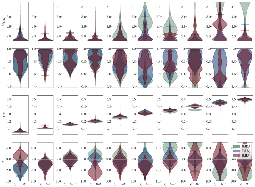
Figure 1: Equal mass configuration $\mathrm{Eq}_{\mathrm{\chi_{\rm eff}}}^{\uparrow\uparrow}$. The extracted posteriors are marked green for the IMRDNRT approximant, red for IMRPNRT, and blue for IMRDNRT_Q. Injected value are marked with a horizontal gray line and $90\%$ confidence intervals are shown with green, red, and blue horizontal lines for the individual approximants.

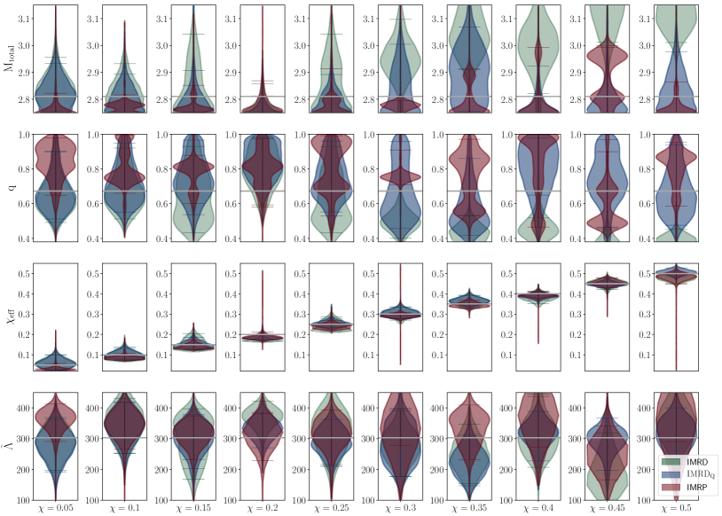
Figure 2: As Fig. 1 but for the unequal-mass configurations $\mathrm{Un}_{\mathrm{\chi_{\rm eff}}}^{\uparrow\uparrow}$.

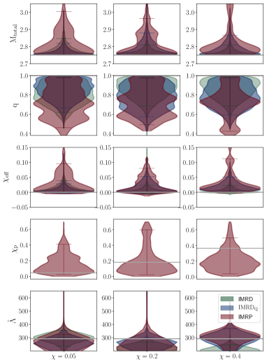
Figure 3: Equal mass system $\mathrm{Eq}_{\mathrm{x}}$ with in in-plane spin $({\leftarrow\rightarrow})$ (left) and with mis-aligned spin $({\nwarrow\nearrow})$ (right). Injected values are marked with a horizontal gray line and $90\%$ confidence intervals are shown with red/green horizontal lines.

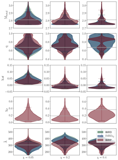
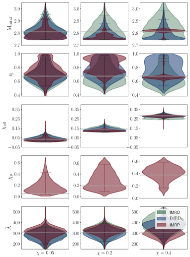
Figure 4: Unequal mass system $\mathrm{Un}_{\mathrm{x}}$ with in in-plane spin ${(\leftarrow\rightarrow})$ (left) and with mis-aligned spin $({\nwarrow\nearrow})$ (right). Injected values are marked with a horizontal gray line and $90\%$ confidence intervals are shown with red/green horizontal lines.

III Extracting intrinsic parameters in presence of spins

In this section, we simulate equal-mass and unequal-mass sources by varying their dimensionless spin magnitudes. Apart from their spins, the intrinsic parameters of each of the equal and unequal mass source are kept fixed and are listed in Tab. 1.

In addition to the priors mentioned above (Sec. II.3), we sample the distance uniformly in a co-moving volume up to $100\rm Mpc$. The priors on the sky position as well as the inclination of the binary are uniformly distributed on the sphere.

III.1 Effects of aligned spins

For each of the sources in Tab. 1, we vary the dimensionless spin magnitudes on each component mass from $0.05$ to $0.5$ in steps of $0.05$. Henceforth, we refer to an aligned-spin equal-mass system with effective spin parameter $\chi_{\rm eff}$ as $\mathrm{Eq}_{\mathrm{\chi_{\rm eff}}}^{\uparrow\uparrow}$. Similarly, the unequal-mass aligned-spinning systems are denoted by $\mathrm{Un}_{\mathrm{\chi_{\rm eff}}}^{\uparrow\uparrow}$.

Equal-mass binaries:

In Fig. 1, we show the posterior probability distribution functions (PDFs) of the intrinsic parameters for each of the injected spin values for the equal-mass setup. Considering the extraction of intrinsic binary properties from the equal-mass binary, we find generally that with IMRPNRT or IMRDNRT_Q the binary parameters are better recovered than for the corresponding IMRDNRT setup. This points to the importance of the spin-spin interactions, in particular for spins $\chi>0.2$.

Independent of the model, for an increasing spin magnitude, the extraction of the total mass, mass ratio, and tidal deformability becomes less restrictive. This is most visible for IMRPNRT when considering the tidal deformability parameter $\tilde{\Lambda}$. Although the injected value (horizontal gray lines for each panel in Fig. 1) lies almost always within the 90% credible interval (given by the colored horizontal lines; the colors corresponding to each waveform approximant), the posterior distribution becomes increasingly broad for larger spins. In comparison, the IMRDNRT_Q model restricts the tidal deformability better than IMRPNRT. A similar effect was discussed in Ref. Samajdar and Dietrich (2018) for non-spinning injections, where it was pointed that the reduction of the parameter space helps to improve the extraction of individual parameters. Trivially, this observation can be generalized to aligned-spin configurations.

With all other parameters being kept fixed, a larger value of $\chi_{\rm eff}$ causes a longer inspiral phase Campanelli et al. (2006); Bernuzzi et al. (2014); Dietrich et al. (2017b). It has been shown Ohme (2012) that effects of larger spin may be compensated by changing values of the mass ratio Baird et al. (2013) or even total mass. We do see a similar trend in the recovered mass ratios as they become smaller for larger spin magnitudes. For these cases, the estimated total masses are higher, which leads to a recovered chirp mass closer to the injected value.

Among the best recovered parameters for all models is the effective aligned-spin parameter $\chi_{\rm eff}$. This can be understood by the fact that the effective spin is mainly determined from the long early-inspiral containing several thousand GW cycles, since the leading order spin-orbit contribution enters already at the 1.5PN order . Only the IMRDNRT approximant shows noticeable differences with respect to the injected values, which again emphasizes the importance of incorporation of the spin-induced quadrupole-monopole term.

It is encouraging that standard waveform approximants are able to determine spin values of $\sim 0.05$ once the design sensitivity of advanced GW detectors is reached. This shows that there is the chance of detecting millisecond pulsars via GW astronomy.

In general, it seems possible to reliably estimate intrinsic parameters up to an aligned spin of $\chi_{\rm eff}\sim 0.4$ once the spin-spin interactions include EOS dependence as in IMRDNRT_Q and IMRPNRT. We note that this value is well above the largest dimensionless spin observed in a BNS system to date ($\chi\sim 0.05$ for PSR J1946+2052 Stovall et al. (2018)), and therefore is also above the low-spin prior of $\chi<0.05$ employed in some of the LVC analyses, e.g. Abbott et al. (2018a, b, c). It is also larger than the dimensionless spin of PSR J1807$-$2500B which is, with a rotation frequency of $239$Hz Lorimer (2008); Lattimer (2012), currently the fastest spinning NS in a binary system.

Unequal-mass binaries:

In Fig. 2, we show the posterior probability distribution functions (PDFs) of the intrinsic parameters for each of the injected spin values for the unequal-mass setup. The results for the unequal-mass configurations are in line with our equal-mass studies. We find that IMRPNRT and IMRDNRT_Q approximants perform best and that above a spin value of $\chi\sim 0.25$ the quadrupolar deformation of the NSs due to its own spin becomes important. Thus, systematic biases are introduced in the IMRDNRT model in which the EOS-dependent quadrupolar deformation is not included. These biases result in a larger estimated total mass and smaller mass ratio (as for the equal-mass case).

Considering the effective spin $\chi_{\rm eff}$, we find that as for the equal mass case the injected value (denoted by horizontal gray lines in each panel in Fig. 2) is recovered robustly and always remains within the 90% credible interval (colored horizontal lines, with the colors corresponding to each waveform approximant). The injected value of $\tilde{\Lambda}$ is always contained within the posterior distribution of the $\tilde{\Lambda}$ parameter for all waveform approximants. As for the equal-mass case, the posterior distribution functions with IMRPNRT recovery broaden with gradual increase in spins. However, the same does not hold true for IMRDNRT_Q recovery.

III.2 Effects of precessing spins

We now consider systems with precession, i.e., setups for which a non-vanishing spin component inside the orbital plane exists. To reduce computational costs, we study only setups for the spin values $\chi=0.05,0.2,0.4$ and discard other spin values studied for the aligned cases.

Equal-mass binaries: The results from the precessing spin equal-mass simulations are shown in Fig. 3. We show in the left panel results for the in-plane configuration and in the right panel results for the misaligned setup.

For the in-plane configuration, the simulated values of total mass $M$ and mass ratio $q$ lie within the $90\%$ upper bound values of their posterior distributions. The effective spin $\chi_{\rm eff}$ is also recovered within the $90\%$ confidence region for in-plane systems although the confidence interval is quite broad to be able to make conclusive statements. For all values of spin magnitudes, recovery with the IMRPNRT model includes the injected value of the precessing spin parameter $\chi_{\rm P}$ within the $90\%$ confidence interval of the posterior distribution. However, the confidence intervals are generally too large to claim confidently a measurement of precession effects. When the injected spin magnitude is large ($\chi\sim 0.4$), we note that IMRDNRT performs poorly to recover the extracted tidal deformability whereas IMRDNRT_Q and IMRPNRT perform similarly, in spite of IMRDNRT_Q being an aligned spinning model.

In an improved model of the NRTidal framework Dietrich et al. , higher order spin-squared and spin-cubed terms are added, along with their respective spin-induced moments. This might improve the estimation of the tidal deformability in the case of large spins.

For the misaligned configurations (right panel of Fig. 3), the total mass $M$ is recovered well with IMRDNRT, but for large spins we find similar biases as for the aligned configuration for IMRDNRT. The $\chi_{\rm eff}$ parameter however, seems to be quite robustly measured. We find the tidal deformability to be loosely constrained with IMRPNRT for this spin orientation.

Overall, our observations might hint towards the fact that a further improvement of the precession dynamics is needed. A possible extension of the IMRPNRT model with a two-spin precession description as in Khan et al. (2018) might help to further improve our capability to extract precession effects from future events. On the other hand, while computationally more expensive, one could also extend the precessing EOB model Pan et al. (2014) with the NRTidal framework to allow a better modelling of the inspiral of precessing BNSs.

Unequal-mass binaries: The results from the simulations of the unequal-mass setup for in-plane (left panel) and misaligned spin (right panel) are shown in Fig. 4. All waveform models include the injected parameters within the $90\%$ confidence intervals of the posterior distributions, although it appears again that $\chi_{\rm eff}$ is slightly overestimated for the $\chi=0.05$ configuration. While most observations made for the equal-mass sources hold also for the unequal-mass sources, we find that for very large misaligned spins ($\chi=0.4$ and the $({\nwarrow\nearrow})$ case) the IMRPNRT posterior of $\chi_{p}$ excludes non-precessing setups. This shows that, as expected, precession effects are easier to detect for unequal mass setups than for equal mass systems.

IV Incorporating information from electromagnetic counterparts

In addition to the study of spin effects, presented in the previous section, we want to understand the possible interplay between GW astronomy and EM observations. For this purpose, we will employ the configurations $\mathrm{Un}_{\mathrm{\chi}}^{(\uparrow\uparrow)}$, $\mathrm{Un}_{\mathrm{\chi}}^{(\leftarrow\rightarrow)}$, $\mathrm{Un}_{\mathrm{\chi}}^{(\nwarrow\nearrow)}$ with $\chi=0.2$ and $0.4$, i.e., a total of six different physical setups. To save further computational costs, we restrict our analysis to the IMRPNRT model since it is the only precessing model and analyse for the observational scenarios II and III (kilonova and GRB respectively, cf. Tab. 2) only the $\chi=0.2$ case and with an aligned-spinning configuration.

GW170817 GBM (2017) has shown the huge variety of EM signals which can be detected in coincidence or as a follow-up of a potential GW trigger. We consider here four different scenarios:

I. the absence of an EM counterpart: For such scenarios one keeps the GW standard priors on the distance and sky location.

II. a kilonova detection: In cases where a kilonova gets detected, the good angular resolution of optical or near-optical telescopes fixes the sky location and provides, due to the redshift measurement of the host galaxy, a constraint on the source distance.

III. a GRB detection: The observation of a GRB generally provides broad information about the sky location. Furthermore, since GRBs are beamed within a small angle, they also provide additional estimates of the inclination of the binary with respect to the line of sight, e.g., Eichler et al. (1989); Paczynski (1991); Narayan et al. (1992); Nathanail (2018); van Eerten et al. (2018); Wu and MacFadyen (2018).

IV. kilonova and GRB detection: As for GW170817 it can be expected that for a number of BNS mergers, one detects both a kilonova and a GRB which combines the constraints of (ii) and (iii).

We provide for all four cases the priors for the distance, sky localization ($\theta,\phi$), and inclination of the system $\iota$ in Tab. 2.

Counterpart	Priors
	$D_{L}\ [\mathrm{Mpc}]$	$\theta\ [\mathrm{deg.}]$	$\phi\ [\mathrm{deg.}]$	$\iota\ [\mathrm{deg.}]$
Injected values	50	60	60	25
No EM counterpart	[1,100]	[0,180]	[-90,90]	[$0$, 180]
Kilonova	[45,55]	fixed	fixed	[$0$, 180]
GRB	[1,100]	[35,85]	[35,85]	[0, 50]
Kilonova + GRB	[45,55]	fixed	fixed	[0, 50]

Table 2: Overview about the prior choices for different observational scenarios considering absence of an EM counterpart, a detection of a kilonova, a detection of a GRB, and the combined detection of a kilonova and a GRB.

For the interpretation of the imprint of the combined EM and GW analyses, we compute the systematic bias with the standard accuracy statistic (stacc) defined as

$$S=\sqrt{\frac{1}{N}\sum_{i=1}^{N}(x_{i}-x_{\mathrm{inj}})^{2}},$$ (8)

where $N$ is the number of samples, $x_{i}$ is the $i^{th}$ posterior sample and $x_{\mathrm{inj}}$ is the injected value of the parameter $x$.

We find that although the covered parameter space is reduced due to the additional EM information, there are only minor changes in the recovered estimates and the incorporation of the source distance, location, and inclination does not noticeably improve the GW data analysis. In fact, there is no obvious systematic improvement in measurement of $\mathrm{M_{total}}$, $\mathrm{q}$ or $\mathrm{\chi_{eff}}$. The only relevant improvement is a better estimate of the tidal deformability. Table 3 shows that for the high spinning configurations if some spin contribution is aligned to the orbital angular momentum, i.e., setups $(\uparrow\uparrow)$ or $({\nwarrow\nearrow})$, the stacc value can be reduced by an order of a few if additional EM information are incorporated.

EM scenario	Spin configuration		Stacc
	Orientation	Spin magnitude	$\tilde{\Lambda}$
no EM	$(\uparrow\uparrow)$	0.20	126.74
no EM	$(\uparrow\uparrow)$	0.40	351.70
kilonova	$(\uparrow\uparrow)$	0.20	99.40
GRB	$(\uparrow\uparrow)$	0.20	56.22
kilonova & GRB	$(\uparrow\uparrow)$	0.20	45.71
kilonova & GRB	$(\uparrow\uparrow)$	0.40	48.13
no EM	$({\leftarrow\rightarrow})$	0.20	59.27
no EM	$({\leftarrow\rightarrow})$	0.40	59.81
kilonova & GRB	$({\leftarrow\rightarrow})$	0.20	109.72
kilonova & GRB	$({\leftarrow\rightarrow})$	0.40	69.15
no EM	$({\nwarrow\nearrow})$	0.20	74.06
no EM	$({\nwarrow\nearrow})$	0.40	110.06
kilonova & GRB	$({\nwarrow\nearrow})$	0.20	50.81
kilonova & GRB	$({\nwarrow\nearrow})$	0.40	44.37

Table 3: Stacc estimtes for different scenarios of combined EM and GW analyses using the IMRPNRT model and the unequal-mass source.

V Summary

In this work, we have presented a first study to classify potential biases in the extraction of binary parameters for spinning and precessing GW signals and how detected EM counterparts can support the GW parameter estimation. Our main findings are summarized as follows:

1. Considering aligned spinning configurations, the effective spin $\chi_{\rm eff}$ is well constrained for all employed waveform approximants. Thus, we might be able to extract information about the spins of the stars from future BNS events.

2. Once the star’s spins exceed values above $\chi\sim 0.2$, GW models need to contain the EOS dependent quadrupole-monopole contribution in the GW phase description, otherwise results are systematically biased.

3. It is unlikely that with the current waveform approximants, precession effects will be detected unless the configuration consists of NSs with different masses and very high spin values.

4. Incorporating additional EM information does not lead to a noticeable improvement of the results, only the tidal deformability changes for some of our investigated configurations.

While this work has only been the first step towards a better understanding of waveform model systematics for spinning, tidal models, it already hints towards possible improvements for future developments. Most notably, we propose the extension of the fully precessing, phenomenological BBH model presented in Khan et al. (2018) to potentially improve our ability to find clear imprints of precession effects from future detections. Furthermore, the noticeable importance of the spin-spin interactions suggest that a more detailed modelling of these effects as presented in Nagar et al. (2018b) for the EOB model or in Dietrich et al. for the NRTidal approximation, should be the focus of future BNS model developments.