Joint Antenna Selection and Hybrid Beamformer Design using Unquantized and Quantized Deep Learning Networks

Abstract

In millimeter wave communications, multiple-input-multiple-output (MIMO) systems use large antenna arrays to achieve high gain and spectral efficiency. These massive MIMO systems employ hybrid beamformers to reduce power consumption associated with fully digital beamforming in large arrays. Further savings in cost and power is possible through use of subarrays. Unlike prior works which resort to large latency methods such as optimization and greedy search for subarray selection, we propose a deep-learning-based approach in order to overcome the complexity issue without causing significant performance loss. We formulate antenna selection and hybrid beamformer design as a classification/prediction problem for convolutional neural networks (CNNs). For antenna selection, the CNN accepts the channel matrix as input and outputs a subarray with an optimal spectral efficiency. The resultant subarray channel matrix is then again fed to a CNN to obtain analog and baseband beamformers. We train the CNNs with several noisy channel matrices that have different channel statistics in order to achieve a robust performance at the network output. Numerical experiments show that our CNN framework provides an order better spectral efficiency and is 10 times faster than the conventional techniques. Further investigations with quantized-CNNs show that the proposed network, saved in no more than 5 bits, is also suited for digital mobile devices.

I Introduction

The conventional cellular communications systems suffer from spectrum shortage while the demand for wider bandwidth and higher data rates is continuously increasing [1]. In this context, millimeter wave (mm-Wave) band, formally defined with the frequency range 30-300 GHz, is a preferred candidate for fifth-generation (5G) communications technology [2, 3, 4, 5]. Compared to sub-6 GHz transmissions envisaged in 5G, the mm-Wave signals encounter a more complex propagation environment that is characterized by higher scattering, severe penetration losses, lower diffraction, and higher path loss for fixed transmitter and receiver gains [1]. These losses are compensated by providing beamforming power gain through massive number of antennas at both transmitter and receiver. Such a massive multiple-input-multiple-output (MIMO) structure [6, 7] enhances the signal-to-noise ratio (SNR) at the reception.

The wide mm-Wave bandwidth enables higher data rates for communications. Since the Nyquist sampling rate is twice the baseband bandwidth, mm-Wave receivers require expensive, high-rate analog-to-digital converters (ADCs) [8, 9]. The power consumption of an ADC increases with the sampling rate, more so at high frequencies [10], for a given architecture. At baseband, each full-resolution ADC consumes $15$-$795$ mW at $36$ MHz-$1.8$ GHz bandwidths. In addition, power consumed by other RF elements such as power amplifiers and data interface circuits in conjunction with large arrays renders it infeasible to utilize a separate radio- and intermediate-frequency (RF-IF) chain for each element. To reduce these cost-power-hardware overheads and yet provide reasonable performance, hybrid beamforming architectures have been proposed for massive MIMO. Here, the signal is processed by both analog and digital beamformers [11, 12, 13, 14, 15].

In the analog processing section of hybrid systems, it is common to employ phase shifters with constant modulus. Using analog switches, which are much simpler and cheaper than the phase shifters, it is possible to further make the overall system more energy-efficient by using subarrays of the larger full antenna array [16, 17]. Optimal selection of subarray elements reduces the power consumption of the analog phase shifters and low-noise amplifiers (LNAs) [18, 19, 20]. Very recent works consider the problem of antenna selection jointly with hybrid beamformer design to optimally trade-off cost and power efficiency [19, 20, 21, 22]. In particular, [21] proposed antenna selection and analog precoder design with low-resolution phase shifters for multiple-input-single-output (MISO) systems. The hybrid beamformer designs suggested in [19] and [20] involve a sub-optimum antenna selection strategy through quadratic approximation with smooth optimization. Similarly, the massive MIMO architecture in [22] employs greedy search for choosing sub-optimal subarrays.

Nearly all of these works provide sub-optimum solutions despite attempting various antenna selection criteria and optimization strategies. Even while using branch-and-bound (BAB) algorithms - which provide good estimation of the lower and upper bounds of regions/branches of the search space in polynomial time - obtaining an optimum solution for massive MIMO subarray selection requires high computational burden [23]. In this paper, to reduce the complexity (in cases where the optimum solution can still be obtained), we introduce an approach based on deep learning (DL) to find an optimum subarray jointly with the design of hybrid beamformers; the optimality is in the sense of achieving maximum spectral efficiency.

As a class of machine learning techniques, DL methods have gained much interest recently for solving many challenging problems such as visual object recognition [24], rainfall estimation [25], and language processing [26]. These techniques offer advantages such as low computational complexity while solving optimization-based or combinatorial search problems as well as the ability to extrapolate new features from a limited set of features contained in a training set [24]. Very recently, DL has received significant attention in addressing problems in communications signal processing such as channel estimation [27], direction-of-arrival (DoA) estimation [28] analog beam selection [29, 30, 31] and beam management in dense mm-Wave networks [32]. At the physical layer of wireless communications, DL has been applied for signal detection [33] and channel estimation [34]. An end-to-end single-input-single-output (SISO) communications scenario is modeled in [34] and [35] by using auto-encoders. In [36], auto-encoders are employed for channel state information (CSI) feedback. A sub-optimum method based on support vector machines (SVMs) is proposed in [28] for selecting analog beamforming vector. In a recent work [37], multilayer perceptrons (MLP) are used for precoder design in a single-user mm-Wave scenario.

In this paper, we exploit DL to simultaneously select antenna elements and design hybrid beamformer. This joint problem as well as the stand-alone hybrid beamforming remain unexamined in the previous DL works. Specifically, we design a convolutional neural network (CNN) to achieve both tasks sequentially. The element selection problem is cast as a classification problem [38]. A similar DL approach was adopted for radar antenna arrays recently in [39]. We further incorporate the hybrid beamformer design in this DL framework by exploiting the structure of analog beamformers which are obtained by minimizing the cost between hybrid and unconstrained beamformers. The optimization problem is cast jointly with the antenna selection problem and it is solved by MATLAB-based Manopt algorithm [40] via manifold optimization (MO) [15].

In our formulation, a CNN accepts channel matrix as input and provides the subarray that maximizes the spectral efficiency. Once the antenna selection is finalized, the corresponding partial channel matrix is fed to a second CNN which then chooses the best RF beamformer and constructs the corresponding baseband beamformer. To train both CNN models, different realizations of the channel matrix are used and the input data are labeled by the selected subarray/RF chains with the highest spectral efficiency. Even though our proposed network structures require channel matrix as an input, precise knowledge of this matrix is only required in the training stage to obtain the labels of the network. In the prediction stage, where the RF beamformers are estimated, precise channel knowledge is not necessary. Both CNNs are trained with channel matrices generated for different user location, channel gains and number of user clusters. Furthermore, each realization of channel matrix in the training data is corrupted by synthetic noise so that the performance of the learning network does not deteriorate with noisy test inputs.

We evaluate the performance of the proposed framework over several experiments and show that proposed CNN approach provides significantly better performance as compared to the optimization and greedy based techniques [14, 9, 37, 41]. In order to account for time-varying channel and user parameters, we use several channel realizations with added noise. We train the networks with huge training data (~240000 input samples) with noisy channel matrices. As a result, the classification accuracy quickly reaches $100\%$ wherein optimum antenna selection and RF beamformer design are accomplished. The CNN is trained offline and, hence, all the computational overhead is taken into account for data generation and training. The classification and prediction time for our proposed approach is at least 10 times faster than the conventional antenna selection techniques as well as hybrid beamformer design algorithms.

Finally, our approach is helpful in reducing the computational burden involved in hybrid beamformers by simply feeding the channel matrix to the network. This requires using CNNs in mobile devices where the data are collected in digital form. Since existing deep neural network models are computationally and memory intensive, they cannot be deployed in devices with low memory resources and low overhead requirements. These constraints have driven investigation into compression of deep neural networks. One of the common approaches is to quantize the CNN weights [42], [43]. In this paper, we investigate the performance of the proposed framework when the weights of the CNNs are quantized. While quantized-CNN structures are recently studied for image classification purposes, ours is the first work that examines quantized-CNNs for communications. Preliminary results of our work appeared in [38] and [42]; while a basic formulation suggested in [38] solved the joint problem for a specific hybrid beamforming scheme, [42] proposed a quantized-CNN approach for the same scheme but did not include antenna selection.

Throughout the paper, we denote the identity matrix of size $N\times N$ as $\mathbf{I}_{N}$. $(\cdot)^{T}$ and $(\cdot)^{H}$ denote transpose and the conjugate transpose operations, respectively. For a matrix $\mathbf{A}$ and a vector $\mathbf{a}$, $[\mathbf{A}]_{:,i}$ and $[\mathbf{A}]_{i,j}$ denote the $i$th column and $(i,j)$th element of matrix $\mathbf{A}$, $[\mathbf{a}]_{i}$ means the $i$th element of vector $\mathbf{a}$, respectively. The notation $|\mathbf{A}|$ denotes the determinant of matrix $\mathbf{A}$ whereas $|a|$ is the absolute value of the scalar $a$. The function $\mathbb{E}\{\cdot\}$ provides the statistical expectation of its argument and $\angle\{\cdot\}$ measures the angle of complex quantity.

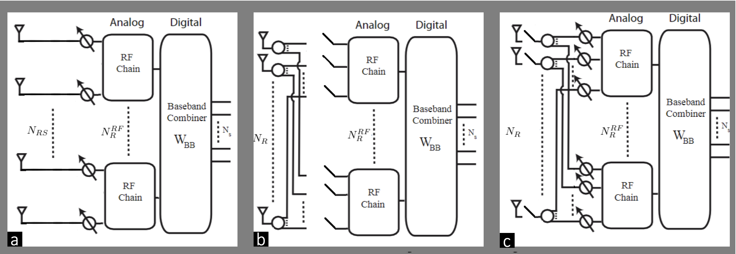
Figure 1: Receiver architectures with antenna selection for single user mmWave MIMO systems. (a) Scheme 1: Fixed subarray with fully-connected phase shifters. (b) Scheme 2: Switching network without optimized antenna selection and no phase shifters. (c) Scheme 3: Switching network with optimized antenna selection and phase shifters.

II System Model For mm-Wave MIMO Systems

Consider a single user mm-Wave MIMO system with $N_{T}$ and $N_{R}$ transmit and receive antennas, respectively (Fig. 1). Assume that $N_{S}$ data streams are desired to be transmitted to the receiver where the antenna selection is performed to select a subarray with $N_{RS}$ antennas out of $N_{R}$. There are $N_{T}^{RF}$ and $N_{R}^{RF}$ RF beamformers at transmit and receive sides such that $N_{S}\leq N_{T}^{RF}\leq N_{T}$ and $N_{S}\leq N_{R}^{RF}\leq N_{RS}\leq N_{R}$. The hybrid precoder structure applies the baseband precoder $\mathbf{F}_{BB}\in\mathbb{C}^{N_{T}^{RF}\times N_{S}}$ to the transmit signal vector $\mathbf{s}\in\mathbb{C}^{N_{S}}$, where $\mathbb{E}\{\mathbf{s}\mathbf{s}^{H}\}=\mathbf{I}_{N_{S}}/N_{S}$. Then, the signal is passed through RF precoders $\mathbf{F}_{RF}\in\mathbb{C}^{N_{T}\times N_{T}^{RF}}$ (constructed using phase shifters) to $N_{T}$ transmit antennas. The RF precoder has equal-norm elements so that $[[\mathbf{F}_{RF}]_{:,i}[\mathbf{F}_{RF}]_{:,i}^{H}]_{i,i}=1/N_{T}$. The power of the transmitter is constrained to $||\mathbf{F}_{RF}\mathbf{F}_{BB}||_{\mathcal{F}}=N_{S}$. The transmitted signal at RF stage is $\mathbf{x}=\mathbf{F}_{RF}\mathbf{F}_{BB}\mathbf{s}\in\mathbb{C}^{N_{T}}$. Assuming a narrowband block-fading channel, the received signal at $N_{R}$ antennas is [44, 14]

$$\mathbf{y}^{\text{Full}}=\sqrt{\rho}\mathbf{H}\mathbf{F}_{RF}\mathbf{F}_{BB}\mathbf{s}+\mathbf{n},$$ (1)

where $\mathbf{y}^{\text{Full}}\in\mathbb{C}^{N_{R}}$ is the output of $N_{R}$ antennas at the receiver, $\rho$ is average received power, $\mathbf{n}\in\mathbb{C}^{N_{R}}$ is the additive white Gaussian noise (AWGN) with $\mathbf{n}\sim\mathcal{CN}(\mathbf{0},\sigma_{n}^{2}\mathbf{I}_{N_{R}})$, and $\mathbf{H}\in\mathbb{C}^{N_{R}\times N_{T}}$ is the channel matrix with $||\mathbf{H}||_{\mathcal{F}}=N_{R}N_{T}$.

A standard analog-digital hybrid beamformer operates on a full array. When a subarray is employed, then beamformers must be derived for reduced dimensions. We model the antenna selection problem to select the best antenna subset from all possible antenna subarrays. Throughout this paper, we use the terms “subarray” and “subset” interchangeably; a subarray being a subset of indices (or antenna positions) of a full array configuration. A popular scheme is to employ a predetermined subarray with $N_{RS}$ antennas is selected from a full array of $N_{R}$ elements (Fig. 1a). Each subarray feeds into a fully-connected phase shifter network of size $N_{R}^{RF}$ with a single RF chain. This has the complexity of phase shifters but the antenna selection process is not optimized. Another common receiver architecture feeds the antennas directly to the RF chains thereby eliminating the phase shifters completely. Here, each RF chain is connected to the $N_{R}$ antennas of which $N_{RS}$ elements are selected using switches (Fig. 1b). In this case, the entries of the combiner matrix are either 1 or 0 to indicate the selected or unselected antennas, respectively. This is the simplest structure with no phase shifters. However, the antenna selection is not optimzed and the elements are determined by simply choosing the largest absolute values in each column of the channel matrix. Finally, Fig. 1c shows a receiver that employs a switching network with phase shifters. In this system, a subarray with $N_{RS}$ antennas is selected from a full array comprising $N_{R}$ antennas. The subarray is connected to a phase shifter network of size $N_{R}^{RF}$ which may apply an optimization procedure for antenna selection to achieve greater efficiency.

Our mm-Wave channel representation is based on the Saleh-Valenzuela (SV) model that utilizes the clustered channel model [45, 46]. Here, the channel matrix $\mathbf{H}$ includes the contributions of $N_{c}$ scattering clusters, each of which has $N_{\text{ray}}$ paths. We have

$$\mathbf{H}=\gamma\sum_{i,j}\alpha_{ij}g_{R}(\Theta_{R}^{(ij)})g_{T}(\Theta_{T}^{(ij)})\mathbf{a}_{R}(\Theta_{R}^{(ij)})\mathbf{a}_{T}^{H}(\Theta_{T}^{(ij)}),$$ (2)

where $\Theta_{R}^{(ij)}=(\phi_{R}^{(ij)},\theta_{R}^{(ij)})$ and $\Theta_{T}^{(ij)}=(\phi_{T}^{(ij)},\theta_{T}^{(ij)})$, respectively, denote the angle of arrivals and angle of departures wherein the azimuth (elevation) angle is denoted by $\phi$ ($\theta$), $\gamma=\sqrt{N_{T}N_{RS}/(N_{\mathrm{c}}N_{\mathrm{ray}})}$ is the normalization factor, and $\alpha_{ij}$ is the complex channel gain associated with the $i$th scattering cluster and $j$th path for $i=1,\dots,N_{\mathrm{c}}$ and $j=1,\dots,N_{\mathrm{ray}}$. The antenna element gains for receive and transmit antennas are $g_{R}(\Theta_{R}^{(ij)})$ and $g_{T}(\Theta_{T}^{(ij)})$, respectively. The steering vector representing the array response at the transmitter (receiver) is $\mathbf{a}_{T}(\Theta_{T}^{(ij)})\in N_{T}\times 1$ ($\mathbf{a}_{R}(\Theta_{R}^{(ij)})\in N_{R}\times 1$). The $n$th element of $\mathbf{a}_{R}(\Theta_{R}^{(ij)})$ is

$$[\mathbf{a}_{R}(\Theta_{R}^{(ij)})]_{n}=\exp\left\{-\frac{2\pi}{\lambda}\mathbf{p}_{n}^{T}\mathbf{r}(\Theta_{R}^{(ij)})\right\},$$ (3)

where $\mathbf{p}_{n}=[x_{n},y_{n},z_{n}]^{T}$ is the position of the $n$th antenna in Cartesian coordinate system and $\mathbf{r}(\Theta_{R}^{(ij)})=[\sin(\phi_{R}^{(ij)})\cos(\theta_{R}^{(ij)}),\sin(\phi_{R}^{(ij)})\sin(\theta_{R}^{(ij)}),\cos(\theta_{R}^{(ij)})]^{T}$. The transmit steering vector $\mathbf{a}_{T}(\Theta_{T}^{(ij)})$ is defined similarly.

In practice, the estimation process of the channel matrix is a challenging task, especially in case of a large number of antennas in massive MIMO systems [47, 48]. Additionally, the mm-Wave channel has short coherence times [49, 1]. In practice, the estimated channel matrix could be obtained via one of the several channel estimation techniques [46, 50, 48, 51, 12]. For robust performance against imperfect channel estimates, our proposed DL framework feeds the deep network with several channel realizations which are corrupted by synthetic noise in the training stage. This is an offline process. Note that the perfect knowledge of channel matrix ${\mathbf{H}}$ is only required at the training stage to obtain the labels (e.g., hybrid beamformer matrices). During the testing stage when the network predicts the beamformer weights, the network does not necessarily require the perfect CSI. Our numerical experiments demonstrate that the proposed approach can handle the corrupted channel matrix case and exhibits satisfactory performance regarding the achievable spectral efficiency.

In the hybrid beamformer, analog and digital beamformers are obtained to maximize the spectral efficiency. Often, this is achieved by exploiting the structure of the mm-Wave channel matrix [51]. Using the full antenna array at the receiver, the received signal in (1) is processed by analog and baseband combiners to yield

$$\bar{\mathbf{y}} =\mathbf{W}_{BB}^{\text{Full}^{H}}\mathbf{W}_{RF}^{\text{Full}^{H}}\mathbf{y}^{\text{Full}}$$

$$=\sqrt{\rho}\mathbf{W}_{BB}^{\text{Full}^{H}}\mathbf{W}_{RF}^{\text{Full}^{H}}\mathbf{H}\mathbf{F}_{RF}\mathbf{F}_{BB}\mathbf{s}+\mathbf{W}_{BB}^{\text{Full}^{H}}\mathbf{W}_{RF}^{\text{Full}^{H}}\mathbf{n},$$ (4)

where $\mathbf{W}_{RF}^{\text{Full}}\in\mathbb{C}^{N_{R}\times N_{R}^{RF}}$ is the analog combiner with the constrained $[[\mathbf{W}_{RF}^{\text{Full}}]_{:,i}[\mathbf{W}_{RF}^{\text{Full}}]_{:,i}^{H}]_{i,i}=1/N_{R}$ and $\mathbf{W}_{BB}^{\text{Full}}\in\mathbb{C}^{N_{R}^{RF}\times N_{S}}$ denotes the baseband combiner matrix. Assuming that the Gaussian symbols are transmitted through the mm-Wave channel, we define the spectral efficiency [14, 11, 12, 13] achieved from the full array as

$$R^{\text{Full}}=\log_{2}\bigg{|}\mathbf{I}_{N_{S}}+\frac{\rho}{N_{S}}\boldsymbol{\Lambda}_{n}^{\text{Full}^{-1}}\mathbf{W}_{BB}^{\text{Full}^{H}}\mathbf{W}_{RF}^{\text{Full}^{H}}\mathbf{H}$$

$$\;\;\;\;\;\;\;\;\;\;\;\;\times\mathbf{F}_{RF}\mathbf{F}_{BB}\mathbf{F}_{BB}^{H}\mathbf{F}_{RF}^{H}\mathbf{H}^{H}\mathbf{W}_{RF}^{\text{Full}}\mathbf{W}_{BB}^{\text{Full}}\bigg{|},$$ (5)

where $\boldsymbol{\Lambda}_{n}^{\text{Full}}=\sigma_{n}^{2}\mathbf{W}_{BB}^{\text{Full}^{H}}\mathbf{W}_{RF}^{\text{Full}^{H}}\mathbf{W}_{RF}^{\text{Full}}\mathbf{W}_{BB}^{\text{Full}}\in\mathbb{C}^{N_{S}\times N_{S}}$ is the covariance matrix of the noise term in (II) after analog combining. We now formulate the problem for subarray selection and obtaining the corresponding analog-digital beamformer in the following section.

III Joint Antenna and RF Chain Selection

Among the antenna selection schemes presented in the previous section, we focus on the Scheme 3 because this architecture requires optimization (the remaining configurations consider selecting a fixed subarray with/without phase shifters). In particular, our goal is to select the outputs of $N_{RS}$ antennas from the full array output $\mathbf{y}^{\text{Full}}$. Consequently, this also requires designing transmit and receive analog and baseband beamformers $\mathbf{F}_{RF}\in\mathbb{C}^{N_{T}\times N_{T}^{RF}}$, $\mathbf{W}_{RF}\in\mathbb{C}^{N_{RS}\times N_{R}^{RF}}$ and $\mathbf{F}_{BB}\in\mathbb{C}^{N_{T}^{RF}\times N_{S}}$, $\mathbf{W}_{BB}\in\mathbb{C}^{N_{R}^{RF}\times N_{S}}$. In other words, the solution of joint antenna selection and hybrid beamformer design satisfies

$$\underset{\mathbf{Q},{\mathbf{F}}_{RF},{\mathbf{F}}_{BB},{\mathbf{W}}_{RF},{\mathbf{W}}_{BB}}{\operatorname*{maximize}}\log_{2}\bigg{|}\mathbf{I}_{N_{S}}+\frac{\rho}{N_{S}\sigma_{n}^{2}}\big{(}\mathbf{W}_{BB}^{H}\mathbf{W}_{RF}^{H}\mathbf{W}_{RF}\mathbf{W}_{BB}\big{)}^{-1}$$

$$\mathbf{W}_{BB}^{H}\mathbf{W}_{RF}^{H}\mathbf{H}_{\mathrm{sub}}\mathbf{F}_{RF}\mathbf{F}_{BB}\mathbf{F}_{BB}^{H}\mathbf{F}_{RF}^{H}\mathbf{H}_{\mathrm{sub}}^{H}\mathbf{W}_{RF}\mathbf{W}_{BB}\bigg{|}$$

$$\;\;\;\;\;\;\;\;\operatorname*{subject\hskip 3.0ptto:}\;\;\;\;\;\;\;\mathbf{F}_{RF}\in\mathcal{F}_{RF},\;\;||\mathbf{F}_{RF}\mathbf{F}_{BB}||_{\mathcal{F}}^{2}=N_{S},$$

$$\;\;\;\;\;\;\;\;\;\;\;\;\;\;\;\;\;\;\;\;\;\;\;\;\;\;\;\;\;\;\;\;\mathbf{W}_{RF}\in\mathcal{W}_{RF},\;\;||\mathrm{diag}\{\mathbf{Q}\}||_{0}=N_{RS},$$ (6)

where $\mathcal{F}_{RF}$ and $\mathcal{W}_{RF}$ denote the feasible sets of analog beamformers, $\mathbf{H}_{\mathrm{sub}}=\mathbf{Q}\mathbf{H}$ is $N_{RS}\times N_{T}$ channel matrix of the selected antennas, and $\mathbf{Q}$ is the $N_{RS}\times N_{R}$ selection matrix whose $(i,j)$th entry is either 1 or 0. Even without antenna selection, the problem in (6) is difficult to solve because of several matrix variables $\mathbf{Q}$, $\mathbf{F}_{RF}$, $\mathbf{W}_{RF}$ and $\mathbf{F}_{BB}$, $\mathbf{W}_{BB}$ [54, 23]. Since obtaining a solution to (6) in real-time is deemed infeasible, we propose a deep learning approach here to achieve an optimum solution with less computational complexity. We first cast the antenna selection stage as a classification problem as follows.

III-A Antenna Selection

In subarray selection, we are interested in picking $N_{RS}$ out of $N_{R}$ elements. This yields ${Q_{A}}=\left(\begin{array}[]{c}N_{R}\\ N_{RS}\end{array}\right)$ possible solutions. Therefore, choosing subarrays can be viewed as a classification problem with ${Q_{A}}$ classes. We define $\mathbb{S}$ as the set of all possible antenna subarray configurations, i.e., $\mathbb{S}=\{\mathbb{S}_{1},\mathbb{S}_{2},\dots,\mathbb{S}_{Q_{A}}\},$ where $\mathbb{S}_{q_{A}}=\{\mathbf{p}_{1}^{q_{A}},\mathbf{p}_{2}^{q_{A}},\dots,\mathbf{p}_{N_{RS}}^{q_{A}}\}$ includes the antenna positions of the ${q_{A}}$th subarray configuration with $q_{A}\in\mathbb{Q}_{A}=\{1,\dots,Q_{A}\}$. Let $\mathbf{y}_{{q_{A}}}$ be an $N_{RS}\times 1$ vector containing the output signal of the selected antennas for the $q_{A}$th subarray configuration of the full array output $\mathbf{y}^{\text{Full}}$ with positions $\mathbb{S}_{q_{A}}$. Then,

$$\mathbf{y}_{q_{A}}=\sqrt{\rho}\mathbf{H}_{{q_{A}}}\mathbf{F}_{RF}\mathbf{F}_{BB}\mathbf{s}+\mathbf{n}_{{q_{A}}},$$ (7)

where $\mathbf{H}_{{q_{A}}}$ is the $N_{RS}\times N_{T}$ channel matrix with selected antennas and $\mathbf{n}_{q_{A}}$ is similarly defined. At the receiver, analog and the baseband combiners - $\mathbf{W}_{RF}\in\mathbb{C}^{N_{RS}\times N_{R}^{RF}}$ and $\mathbf{W}_{BB}\in\mathbb{C}^{N_{R}^{RF}\times N_{S}}$, respectively - are applied to the received signal to produce the $N_{S}\times 1$ discrete-time signal $\bar{\mathbf{y}}_{q_{A}}=\mathbf{W}_{BB}^{H}\mathbf{W}_{RF}^{H}\mathbf{y}_{{q_{A}}}$ as

$$\bar{\mathbf{y}}_{q_{A}}=\sqrt{\rho}\mathbf{W}_{BB}^{H}\mathbf{W}_{RF}^{H}\mathbf{H}_{q_{A}}\mathbf{F}_{RF}\mathbf{F}_{BB}\mathbf{s}+\mathbf{W}_{BB}^{H}\mathbf{W}_{RF}^{H}\mathbf{n}_{{q_{A}}}.$$ (8)

When the ${q_{A}}$th subarray is selected, the spectral efficiency [55] of the mm-Wave channel is

$$R({q_{A}})=\log_{2}\bigg{|}\mathbf{I}_{N_{S}}+\frac{\rho}{N_{S}}\boldsymbol{\Lambda}_{n}^{-1}\mathbf{W}_{BB}^{H}\mathbf{W}_{RF}^{H}\mathbf{H}_{q_{A}}$$

$$\times\mathbf{F}_{RF}\mathbf{F}_{BB}\mathbf{F}_{BB}^{H}\mathbf{F}_{RF}^{H}\mathbf{H}_{q_{A}}^{H}\mathbf{W}_{RF}\mathbf{W}_{BB}\bigg{|},$$ (9)

where $\boldsymbol{\Lambda}_{n}=\sigma_{n}^{2}\mathbf{W}_{BB}^{H}\mathbf{W}_{RF}^{H}\mathbf{W}_{RF}\mathbf{W}_{BB}\in\mathbb{C}^{N_{S}\times N_{S}}$ corresponds to the noise term of the subarray output in (7). Note that $R({q_{A}})$ depends on $q_{A}$ through $\mathbf{H}_{q_{A}}$. By maximizing the spectral efficiency in (III-A) over all subarray configurations, the best antenna subarray is obtained as

$$\bar{q}_{A}=\operatorname*{argmax}_{q_{A}\in\mathbb{Q}_{A}}R(q_{A}),$$ (10)

where $\bar{q}_{A}$ denotes the subarray index with antenna positions $\mathbb{S}_{\bar{q}_{A}}$ which provide the maximum spectral efficiency.

While the optimization problem in (10) yields the best subarray configuration, it does not impose any constraint on the hybrid beamformers. Here the problem in (10) is cast by using unconstrained beamformers $\mathbf{F}_{q_{A}}^{\mathrm{opt}}\in\mathbb{C}^{N_{T}\times N_{S}}$ and $\mathbf{W}_{q_{A}}^{\mathrm{opt}}\in\mathbb{C}^{N_{RS}\times N_{S}}$. These can be obtained from the singular value decomposition (SVD) of the ${N_{RS}\times N_{T}}$ complex-valued channel matrix: $\mathbf{H}_{q_{A}}=\mathbf{U}_{q_{A}}\boldsymbol{\Sigma}_{q_{A}}\mathbf{V}_{q_{A}}^{H}$, where $\mathbf{U}_{q_{A}}\in\mathbb{C}^{N_{RS}\times\mathrm{rank}(\mathbf{H}_{q_{A}})}$ and $\mathbf{V}_{q_{A}}\in\mathbb{C}^{N_{T}\times\mathrm{rank}(\mathbf{H}_{q_{A}})}$ are the left and the right singular value matrices of the ${q_{A}}$th channel matrix, respectively, and $\boldsymbol{\Sigma}_{q_{A}}$ is $\mathrm{rank}(\mathbf{H}_{q_{A}})\times\mathrm{rank}(\mathbf{H}_{q_{A}})$ matrix composed of the singular values of $\mathbf{H}_{q_{A}}$ in descending order. By decomposing $\boldsymbol{\Sigma}_{q_{A}}$ and $\mathbf{V}_{q_{A}}$ as $\boldsymbol{\Sigma}_{q_{A}}=\text{diag}\{\boldsymbol{\Sigma}_{q_{A}}^{(1)},\boldsymbol{\Sigma}_{{q_{A}}}^{(2)}\},\hskip 5.0pt\mathbf{V}_{q_{A}}=[\mathbf{V}_{{q_{A}}}^{(1)},\mathbf{V}_{{q_{A}}}^{(2)}],$ where $\mathbf{V}_{{q_{A}}}^{(1)}\in\mathbb{C}^{N_{T}\times N_{S}}$ and $\mathbf{V}_{{q_{A}}}^{(2)}\in\mathbb{C}^{N_{T}\times N_{RS}-N_{S}}$, one can readily select the unconstrained precoder as $\mathbf{F}_{q_{A}}^{\text{opt}}=\mathbf{V}_{{q_{A}}}^{(1)}$ [14]. Using the unconstrained beamformer $\mathbf{F}_{q_{A}}^{\mathrm{opt}}$, $\mathbf{W}_{q_{A}}^{\mathrm{opt}}$ is computed as [56]

$$\mathbf{W}_{q_{A}}^{\mathrm{opt}}=\bigg{(}\frac{1}{\rho}\big{(}\mathbf{F}_{q_{A}}^{\mathrm{opt}^{H}}\mathbf{H}_{q_{A}}^{H}\mathbf{H}_{q_{A}}\mathbf{F}_{q_{A}}^{\mathrm{opt}}+\frac{N_{S}\sigma_{n}^{2}}{\rho}\mathbf{I}_{N_{S}}\big{)}^{-1}\mathbf{F}_{q_{A}}^{\mathrm{opt}^{H}}\mathbf{H}_{q_{A}}^{H}\bigg{)}^{H}.$$

Using $\mathbf{F}_{q_{A}}^{\mathrm{opt}}$ and $\mathbf{W}_{q_{A}}^{\mathrm{opt}}$, the following problem can be written, i.e.,

$$\underset{q_{A}\in\mathbb{Q}_{A}}{\operatorname*{maximize}}\;\log_{2}\bigg{|}\mathbf{I}_{N_{S}}+\frac{\rho}{N_{S}\sigma_{n}^{2}}\big{(}\mathbf{W}_{q_{A}}^{\mathrm{opt}^{H}}\mathbf{W}_{q_{A}}^{\mathrm{opt}}\big{)}^{-1}\mathbf{W}_{q_{A}}^{\mathrm{opt}^{H}}\mathbf{H}_{q_{A}}$$

$$\;\;\;\;\;\;\;\;\;\;\;\;\;\;\;\;\;\;\;\;\times\mathbf{F}_{q_{A}}^{\mathrm{opt}}\mathbf{F}_{q_{A}}^{\mathrm{opt}^{H}}\mathbf{H}_{q_{A}}^{H}\mathbf{W}_{q_{A}}^{\mathrm{opt}}\bigg{|}.$$ (11)

The optimization problem in (11) uses unconstrained beamformers $\mathbf{F}^{\mathrm{opt}}$, $\mathbf{W}^{\mathrm{opt}}$ for antenna selection and hybrid beamformer design. However, the ”best” subarray obtained from (11) would be different if hybrid beamformers are used in the problem. Hence, we consider the joint problem with hybrid beamformers and write the joint antenna selection and hybrid beamformer design problem as

$$\underset{q_{A}\in\mathbb{Q}_{A}}{\operatorname*{maximize}}\log_{2}\bigg{|}\mathbf{I}_{N_{S}}+\frac{\rho}{N_{S}\sigma_{n}^{2}}\big{(}\mathbf{W}_{BB_{q_{A}}}^{H}\mathbf{W}_{RF_{q_{A}}}^{H}\mathbf{W}_{RF_{q_{A}}}\mathbf{W}_{BB_{q_{A}}}\big{)}^{-1}\mathbf{W}_{BB_{q_{A}}}^{H}$$

$$\times\mathbf{W}_{RF_{q_{A}}}^{H}\mathbf{H}_{q_{A}}\mathbf{F}_{RF_{q_{A}}}\mathbf{F}_{BB_{q_{A}}}\mathbf{F}_{BB_{q_{A}}}^{H}\mathbf{F}_{RF_{q_{A}}}^{H}\mathbf{H}_{q_{A}}^{H}\mathbf{W}_{RF_{q_{A}}}\mathbf{W}_{BB_{q_{A}}}\bigg{|}$$

$$\operatorname*{subject\hskip 3.0ptto:}\;\;\;\mathbf{F}_{RF_{q_{A}}}\in\mathcal{F}_{RF},\;\;||\mathbf{F}_{RF_{q_{A}}}\mathbf{F}_{BB_{q_{A}}}||_{\mathcal{F}}^{2}=N_{S},$$

$$\;\;\;\;\;\;\;\;\;\;\;\;\;\;\;\;\;\;\;\;\mathbf{W}_{RF_{q_{A}}}\in\mathcal{W}_{RF},$$ (12)

which requires to solve hybrid beamformer design problem for each $q_{A}\in\mathbb{Q}_{A}$. Let us, for now, assume that the hybrid beamformers are estimated as described in the next subsection. Then, the antenna subarray that provides the maximum spectral efficiency is obtained and this subarray is represented by the subarray index $\bar{q}_{A}$. When the problem in (12) is solved for different channel matrices, some of the $\bar{q}_{A}$ values turn out to be the same for different channel matrices which are similar to each other and the same antenna subarray provides the maximum spectral efficiency for these channel matrices [39]. As a result, the number of subarrays providing the maximum spectral efficiency, say $\bar{Q}_{A}$, is much less than the number of all subarray configurations, i.e., $\bar{Q}_{A}\ll Q_{A}$. In [39], a similar observation is made for cognitive radar scenario. Therefore, we define another subset of subarray configurations as $\mathbb{A}=\{\mathbb{A}_{1},\dots,\mathbb{A}_{\bar{Q}_{A}}\},$ which is composed of the subarrays providing maximum spectral efficiency for different channel matrices. In other words, $\mathbb{A}_{\bar{q}_{A}}$ includes the antenna positions of the subarray obtained by solving (11), hence we have $\mathbb{A}\subset\mathbb{S}$.

For very large number of antennas, say, $N_{R}>64$, the computation of all possible antenna subsets is computationally prohibitive and requires very large amount of memory. To tackle this problem, we use close-to-optimum branch-and-bound (BAB) techniques [23]. To further reduce the complexity, we also partition $\mathbb{S}$ into $B$ non-overlapping blocks as $\mathbb{S}^{(b)}=\mathbb{S}_{N_{A}(b-1)+1},\dots,\mathbb{S}_{N_{A}b}$ where $N_{A}$ is the block size and $b=1,\dots,B$. Then the antenna selection problem is solved for $N_{A}$ nodes at a times hence less memory is used. In particular, the following strategy is used:

1. For $b=1$, construct $\mathbb{S}^{(b)}$ and solve (12) as $\bar{q}_{A}^{(b)}=\operatorname*{argmax}_{q_{A}\in\mathbb{S}^{(b)}}R(q_{A})$.

2. For $b>1$, clear $\mathbb{S}^{(b-1)}$ from the memory and construct $\mathbb{S}^{(b)}$, then solve (12) as $\bar{q}_{A}^{(b)}=\operatorname*{argmax}_{q_{A}\in\mathbb{S}^{(b)}}R(q_{A})$ and obtain the new best subarray index as

   $$\bar{q}_{A}^{(b)}:=\left\{\begin{array}[]{ll}\bar{q}_{A}^{(b)},&\mathrm{if}\;R(\bar{q}_{A}^{(b-1)})<R(\bar{q}_{A}^{(b)})\\ \bar{q}_{A}^{(b-1)},&\mathrm{otherwise}\end{array}\right..$$ (15)

III-B Hybrid Beamformer Design

In (12), antenna selection is performed by estimating the beamformer weights for each $q_{A}$. Let $\mathbf{H}_{q_{A}}\in\mathbb{C}^{N_{RS}\times N_{T}}$ be the selected channel matrix, then the hybrid design problem can be written as

$$\underset{\mathbf{F}_{RF},\mathbf{F}_{BB},\mathbf{W}_{RF},\mathbf{W}_{BB}}{\operatorname*{maximize}}\log_{2}\bigg{|}\mathbf{I}_{N_{S}}+\frac{\rho}{N_{S}\sigma_{n}^{2}}\big{(}\mathbf{W}_{BB}^{H}\mathbf{W}_{RF}^{H}\mathbf{W}_{RF}\mathbf{W}_{BB}\big{)}^{-1}$$

$$\;\;\;\;\;\;\;\;\;\;\;\;\;\times\mathbf{W}_{BB}^{H}\mathbf{W}_{RF}^{H}\mathbf{H}_{{q}_{A}}\mathbf{F}_{RF}\mathbf{F}_{BB}\mathbf{F}_{BB}^{H}\mathbf{F}_{RF}^{H}\mathbf{H}_{{q}_{A}}^{H}\mathbf{W}_{RF}\mathbf{W}_{BB}\bigg{|}$$

$$\;\operatorname*{subject\hskip 3.0ptto:}\mathbf{F}_{RF}\in\mathcal{F}_{RF},||\mathbf{F}_{RF}\mathbf{F}_{BB}||_{\mathcal{F}}^{2}=N_{S},\mathbf{W}_{RF}\in\mathcal{W}_{RF}.$$ (16)

Above problem can be written as two decoupled optimization problems to find precoders and combiners separately [14, 15]. In this case, the Euclidean distance between the unconstrained beamformers and the hybrid beamformers is minimized. In other words, the hybrid precoder design problem can be written as follows

$$\underset{\mathbf{F}_{RF},\mathbf{F}_{BB}}{\operatorname*{minimize}}\;\;\;||\mathbf{F}_{q_{A}}^{\mathrm{opt}}-\mathbf{F}_{RF}\mathbf{F}_{BB}||_{\mathcal{F}}^{2}$$

$$\operatorname*{subject\hskip 3.0ptto:}\;\;\mathbf{F}_{RF}\in\mathcal{F}_{RF}.$$ (17)

In a similar way, the combiner design problem can be written as

$$\underset{{\mathbf{W}}_{RF},\mathbf{W}_{BB}}{\operatorname*{minimize}}\;\;\;||{\mathbf{W}}_{q_{A}}^{\mathrm{opt}}-{\mathbf{W}}_{RF}\mathbf{W}_{BB}||_{\mathcal{F}}^{2}$$

$$\operatorname*{subject\hskip 3.0ptto:}\;{\mathbf{W}}_{RF}\in{\mathcal{W}}_{RF},$$

$$\;\;\;\;\;\;\mathbf{W}_{BB}=(\mathbf{W}_{RF}^{H}\boldsymbol{\Lambda}_{{{q}}_{A}}\mathbf{W}_{RF})^{-1}(\mathbf{W}_{RF}^{H}\boldsymbol{\Lambda}_{{{q}}_{A}}\mathbf{W}_{{{q}}_{A}}^{\mathrm{opt}}),$$ (18)

where $\boldsymbol{\Lambda}_{{{q}}_{A}}=\frac{\rho}{N_{S}}\mathbf{H}_{{{q}}_{A}}\mathbf{F}_{RF}\mathbf{F}_{BB}\mathbf{F}_{BB}^{H}\mathbf{F}_{RF}^{H}\mathbf{H}_{{{q}}_{A}}^{H}+\sigma_{n}^{2}\mathbf{I}_{N_{RS}},$ denotes the covariance of the array output in (7) corresponding to the selected subarray index ${{{q}}_{A}}$.

Above optimization problems in (17) and (III-B) can be effectively solved by MATLAB-based Manopt algorithm [40] via manifold optimization [15]. Once we obtain $\mathbf{F}_{RF},\mathbf{F}_{BB}$ and $\mathbf{W}_{RF},\mathbf{W}_{BB}$, the labels of the output layer of the network can be formed as

$$\mathbf{z}=[\mathrm{vec}^{T}\{\angle\mathbf{F}_{RF}\},\operatorname{Re}\{\mathrm{vec}^{T}\{\mathbf{F}_{BB}\}\},\operatorname{Im}\{\mathrm{vec}^{T}\{\mathbf{F}_{BB}\}\},$$

$$\;\mathrm{vec}^{T}\{\angle\mathbf{W}_{RF}\},\operatorname{Re}\{\mathrm{vec}^{T}\{\mathbf{W}_{BB}\}\},\operatorname{Im}\{\mathrm{vec}^{T}\{\mathbf{W}_{BB}\}\}]^{T},$$ (19)

which is a $G\times 1$ real-valued vector and $G=N_{T}N_{T}^{RF}+N_{RS}N_{R}^{RF}+2N_{S}(N_{T}^{RF}+N_{R}^{RF})$.

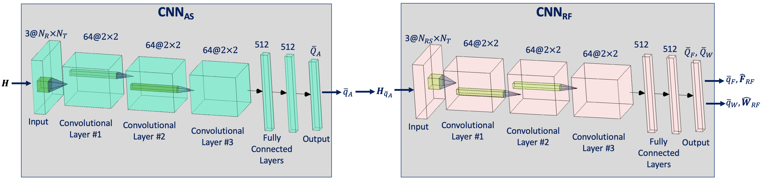
Figure 2: The proposed CNN architecture for antenna selection and RF beamformer design.

Even with the above memory-friendly approach, it is still computationally complex to search all possible antenna subsets in real-time. In order to circumvent this problem, we design a deep learning approach where the network is trained offline with the overhead containing the computation of all possible subarray and RF chain combinations. Then, the trained network can simply be employed as a classification network to select the best antenna subarray and the corresponding RF beamformers for the given channel matrix. We introduce the proposed deep learning technique in the following section.

IV Training the DL Network

The proposed deep network comprises two CNNs (Fig. 2). The first (CNN_AS) accepts the input of channel matrix with the goal to select best antenna subarray $\bar{q}_{A}$. The second CNN (CNN_RF) takes the input of the subsequent channel matrix with selected rows to choose RF beamformers. For both CNNs, training data are selected from different channel matrix realizations each of which is assigned with the corresponding output classes.

Let $\mathbf{X}$ be $N_{R}\times N_{T}\times 3$ input data of the network with $c=3$ channels. We define the first channel of the input as the absolute value of the imperfect channel matrix $\tilde{\mathbf{H}}$ as $[[\mathbf{X}]_{:,:,1}]_{i,j}=|[\tilde{\mathbf{H}}]_{i,j}|$ where $\tilde{\mathbf{H}}\sim\mathcal{CN}(\mathbf{H},\boldsymbol{\Gamma})$. $\boldsymbol{\Gamma}\in\mathbb{R}^{N_{R}\times N_{T}}$ denotes the variance of AWGN with its $(i,j)$th entry as $\boldsymbol{\Gamma}_{i,j}=\frac{10^{\text{SNR}_{\mathrm{TRAIN}}/20}}{[\mathbf{H}]_{i,j}}$ where $\text{SNR}_{\mathrm{TRAIN}}$ denotes the SNR for the AWGN in the training process. Similarly, the second and the third channels are defined as the real and imaginary parts of $\tilde{\mathbf{H}}$, i.e., $[[\mathbf{X}]_{:,:,2}]_{i,j}=\operatorname{Re}\{[\tilde{\mathbf{H}}]_{i,j}\}$ and $[[\mathbf{X}]_{:,:,3}]_{i,j}=\operatorname{Im}\{[\tilde{\mathbf{H}}]_{i,j}\}$. We generate $NL$ realizations of the channel matrix where $N$ different channel matrices are generated with different user locations and channel gains. Each channel matrix is generated for $L_{\mathrm{c}}$ different number of cluster to enrich the training data. In addition, the channel matrix is corrupted by synthetic noise for $L_{\mathrm{n}}$ realizations where the element-wise noise is defined by $\text{SNR}_{\text{TRAIN}}$. Hence, the total size of the training input data is $N_{R}\times N_{T}\times 3\times NL$ where $L=L_{\mathrm{c}}L_{\mathrm{n}}$. For each generated channel matrix, say ${\mathbf{H}}^{(n)}$, the best antenna subarrays with positions $\mathbb{A}_{\bar{q}_{A}}$ and the best RF beamformers $\mathbf{F}_{RF},\mathbf{W}_{RF}$ are obtained by solving (11), (17) and (III-B) offline. This gives input-output pairs of the training data. The training process of both CNNs is identical except that they have different input dimensions. Algorithm 1 summarizes the steps of training data generation.

1:Input: $L_{\mathrm{c}}$, $L_{\mathrm{n}}$, $N$, $N_{T}$, $N_{R}$, $N_{RS}$, SNR${}_{\text{TRAIN}}$.

2:Output: Training data $\mathcal{D}_{\mathrm{AS}}$ and $\mathcal{D}_{\mathrm{RF}}$.

3:Initialize with $t=1$ for $t=1,\dots,T=NL$ where $L=L_{\mathrm{c}}L_{\mathrm{n}}$.

4:for $1\leq n\leq N$ do

5:for $1\leq l_{\mathrm{c}}\leq L_{\mathrm{c}}$ do

6:Generate $\mathbf{H}^{(l_{\mathrm{c}},n)}$ with $N_{\mathrm{c}}=\mathbb{N}_{\mathrm{cluster}}^{({l_{\mathrm{c}})}}$.

7:for $1\leq l\leq L_{\mathrm{n}}$ do

8:$[\mathbf{H}^{(t)}]_{i,j}\sim\mathcal{CN}([\mathbf{H}^{(l_{\mathrm{c}},n)}]_{i,j},\sigma_{\text{TRAIN}}^{2})$.

9:for $1\leq q_{A}\leq Q_{A}$ do

10:$\mathbf{H}_{q_{A}}^{(t)}=\mathbf{U}_{q_{A}}^{(t)}\boldsymbol{\Sigma}_{q_{A}}^{(t)}\mathbf{V}_{q_{A}}^{(t)^{H}}$.

11:$\mathbf{F}_{{{q}}_{A}}^{\mathrm{opt}^{(t)}}=\mathbf{V}_{{q}_{A}}^{(1)^{(t)}}$ .

12:$\mathbf{W}_{{{q}}_{A}}^{\mathrm{opt}^{(t)}}=\bigg{(}\frac{1}{\rho}\big{(}\mathbf{F}_{q_{A}}^{\mathrm{opt}^{(t)^{H}}}\mathbf{H}_{q_{A}}^{(t)^{H}}\mathbf{H}_{q_{A}}^{(t)}\mathbf{F}_{q_{A}}^{\mathrm{opt}^{(t)}}$$+\frac{N_{S}\sigma_{n}^{2}}{\rho}\mathbf{I}_{N_{S}}\big{)}^{-1}\mathbf{F}_{q_{A}}^{\mathrm{opt}^{(t)^{H}}}\mathbf{H}_{q_{A}}^{(t)^{H}}\bigg{)}^{H}$.

13:Use $\mathbf{F}_{{{q}}_{A}}^{\mathrm{opt}^{(t)}}$, and find ${\mathbf{F}}_{RF_{q_{A}}}^{(t)}$, ${\mathbf{F}}_{BB_{q_{A}}}^{(t)}$ by solving (17).

14:Use $\mathbf{W}_{{{q}}_{A}}^{\mathrm{opt}^{(t)}}$, and find ${\mathbf{W}}_{RF_{q_{A}}}^{(t)}$, ${\mathbf{W}}_{BB_{q_{A}}}^{(t)}$ in (III-B).

15:Compute $R_{A}^{(t)}(q_{A})$ in (III-A).

16:end for

17:$\mathbf{H}_{\bar{q}_{A}}^{(t)}\leftarrow\bar{q}_{A}^{(t)}=\arg\max_{q_{A}}R_{A}^{(t)}(q_{A})$.

18:$\mathbf{F}_{RF}^{(t)}\leftarrow{\mathbf{F}}_{RF_{\bar{q}_{A}}}^{(t)}$, $\mathbf{F}_{BB}^{(t)}\leftarrow{\mathbf{F}}_{BB_{\bar{q}_{A}}}^{(t)}$.

19:$\mathbf{W}_{RF}^{(t)}\leftarrow{\mathbf{W}}_{RF_{\bar{q}_{A}}}^{(t)}$., $\mathbf{W}_{BB}^{(t)}\leftarrow{\mathbf{W}}_{BB_{\bar{q}_{A}}}^{(t)}$.

20:$[[\mathbf{X}^{(t)}]_{:,:,1}]_{i,j}=|[\mathbf{H}^{(t)}]_{i,j}|$.

21:$[[\mathbf{X}^{(t)}]_{:,:,2}]_{i,j}=\operatorname{Re}\{[\mathbf{H}^{(t)}]_{i,j}\}$ .

22:$[[\mathbf{X}^{(t)}]_{:,:,3}]_{i,j}=\operatorname{Im}\{[\mathbf{H}^{(t)}]_{i,j}\}$ $\forall ij$.

23:$\mathbf{z}^{(t)}=[\mathrm{vec}^{T}\{\angle\mathbf{F}_{RF}^{(t)}\},\operatorname{Re}\{\mathrm{vec}^{T}\{\mathbf{F}_{BB}^{(t)}\}\},\operatorname{Im}\{\mathrm{vec}^{T}\{\mathbf{F}_{BB}^{(t)}\}\},$ $\mathrm{vec}^{T}\{\angle\mathbf{W}_{RF}^{(t)}\},\operatorname{Re}\{\mathrm{vec}^{T}\{\mathbf{W}_{BB}^{(t)}\}\},\operatorname{Im}\{\mathrm{vec}^{T}\{\mathbf{W}_{BB}^{(t)}\}\}]^{T}.$

24:Construct the input-output pair $(\mathbf{X}^{(t)},\bar{q}_{A}^{(t)})$ for CNN${}_{\text{AS}}$ and $(\mathbf{X}_{\bar{q}_{A}}^{(t)},\mathbf{z}^{(t)})$ for CNN${}_{\text{RF}}$.

25:$t\leftarrow t+1.$

26:end for

27:end for

28:end for

29:Training data for CNN${}_{\text{AS}}$ and CNN${}_{\text{RF}}$ is obtained from the collection of the input-output pairs as $\mathcal{D}_{\mathrm{AS}}=((\mathbf{X}^{(1,1)},\bar{q}_{A}^{(1,1)}),\dots,(\mathbf{X}^{(T)},\bar{q}_{A}^{(T)}))$, $\mathcal{D}_{\mathrm{RF}}=((\mathbf{X}_{\bar{q}_{A}}^{(1,1)},\mathbf{z}^{(1,1)}),\dots,(\mathbf{X}_{\bar{q}_{A}}^{(T)},\mathbf{z}^{(T)})).$

Algorithm 1 Training data generation for CNN_AS and CNN_RF.

(a)

(b)

(c)

(d)

Figure 3: Performance of CNN. (a) Validation loss versus number of channel realizations $L_{\mathrm{n}}$. (b) Validation loss for CNN_RF and validation accuracy for CNN_AS. (c) Spectral efficiency versus number of clusters in when $\sigma_{\Theta}^{2}=5^{\circ}$. (d) Spectral efficiency versus angle spread when $N_{\mathrm{c}}=4$. We set $N_{T}=N_{R}=64$ and $N_{S}=4$ for all figures and $N_{RS}=16$ in (a), (c) and (d).

The CNN${}_{\text{AS}}$ accepts the input of size $N_{R}\times N_{T}\times 3$ with labels $q_{A}$ whereas the input of CNN${}_{\text{RF}}$ is of size $N_{RS}\times N_{T}\times 3$ with label $\mathbf{z}$. For each CNN, the network is composed of $14$ layers. The first layer is the input layer with appropriate size. The second, fourth and the sixth layers are convolutional layers with $64$ filters of size $2\times 2$. The eight and eleventh layers are fully connected layers with $512$ units. The tenth and thirteenth layers are dropout layers with $50\%$ probability placed after each fully connected layers. There are ReLU (Rectified Linear Unit) layers after each convolutional and fully connected layers where ReLU$(x)=\max(x,0)$. The final layer of CNN_AS is the classification layer with size $\bar{Q}_{A}$ which is the number of subarrays that yield maximum spectral efficiency. In the classification layer, a softmax function is used to obtain the probability distribution of the classes. The output layer of CNN_RF is a regression layer of size $G\times 1$. The proposed network is realized in MATLAB on a PC with 768-core GPU. The proposed network architecture is obtained through an optimization analysis to achieve the best performance and less computational cost.

The use of neural networks in mobile devices is also another issue for practical considerations since a deep neural network is composed of huge number of weights for each layers such as convolutional and fully connected layers [43]. The proposed CNN framework should be applied to the channel matrix in a mobile device to obtain hybrid beamformers where the resolution of the network parameters is of great importance. In common CNN architectures, convolutional layers have relatively less parameter to be optimized as compared to the fully connected layers which have large number of neurons to be updated in each iteration [57]. In order to obtain low resolution CNN structure, each of the weights and bias of all layers are quantized so that the saving in the memory is achieved and the implementation of the CNN is eased.

To train the proposed CNN structure, $N=100$ different realizations of the channel matrix which is generated for $L=800$ ($L_{\mathrm{c}}={4}$ for $N_{\mathrm{c}}\in\mathbb{N}_{\mathrm{cluster}}=\{3,4,5,6\}$ and $L_{\mathrm{n}}=200$) noisy realizations with three noise levels, i.e., $\text{SNR}_{\text{TRAIN}}\in\{15,20,25\}$dB. Hence the total size of the training data is $N_{R}\times N_{T}\times 3\times 240000$. In the training process, $70\%$ and $30\%$ of all data generated are selected as the training and validation datasets, respectively. Validation aids in hyperparameter tuning during the training phase to avoid the network simply memorizing the training data rather than learning general features for accurate prediction with new data. The validation data is used to test the performance of the network in the simulations for $J_{T}=100$ Monte Carlo trials.

V Numerical Experiments

We evaluated the performance of the proposed CNN approach via several experiments. In order to prevent the similarity between the test data and the training data we also add synthetic noise to the test data where the SNR in testing is defined similar to $\text{SNR}_{\text{TRAIN}}$ as $\text{SNR}_{\text{TEST}}=20\log_{10}(\frac{|[\mathbf{H}]_{i,j}|^{2}}{\boldsymbol{\Gamma}_{i,j}})$. We used the stochastic gradient descent algorithm with momentum [58] for updating the network parameters with learning rate $0.01$ and mini-batch size of $500$ samples for 50 epochs. As a loss function, we use the negative log-likelihood or cross-entropy loss [24]. We select $N_{T}^{RF}=N_{R}^{RF}=4$ for all simulations. For each channel matrix realization, the propagation environment is modeled with $N_{\mathrm{c}}=4$ clusters and $N_{\mathrm{ray}}=5$ rays for each clusters with the angle spread of $\sigma_{\Theta}^{2}=5^{\circ}$ for all transmit and receive azimuth and elevation angles which are uniform randomly selected from the interval $[-60^{\circ},60^{\circ}]$ and $[-20^{\circ},20^{\circ}]$ respectively.

V-A Performance of Unquantized CNN

Figure 3 summarizes our assessment of the performance of unquantized CNN. Here, we set $N=100$, $N_{T}=N_{R}=64$ and $N_{S}=4$. Figure 3a shows the validation loss of CNN_RF against the number of noisy channel realizations $L$. We observe that the loss is satisfactory for $L\geq 150$; in our simulations, we keep $L=200$. Note that this is a common result for different number of channel realizations $N$. In fact, we use $N=100$ in our settings to achieve reasonable network accuracy. To investigate the performance of deep networks against different noise levels in the training data, we demonstrate the validation loss of CNN_RF and the classification accuracy of CNN_AS in Fig. 3b for different $N_{RS}$ values. It is clear here that both networks attain satisfactory network accuracy for SNR${}_{\mathrm{TEST}}\geq 0$dB. At low SNR regimes, CNN has poor classification performance due to the deviations between the input and the channel matrices used in the training data. In order to make CNN more robust to noisy inputs, we draw the training data for multiple SNR${}_{\text{TRAIN}}$ levels. Nevertheless, noise in the training data expectedly limits the performance since the network cannot distinguish the input data if it is corrupted too much. This issue is also reported in [39, 59] for multiple SNR${}_{\text{TRAIN}}$ case.

The channel statistics are important parameters that change in very short time in mm-Wave channels. Hence, in the training stage, we feed the network with channel realizations of different $N_{\mathrm{c}}$ values. To further investigate the performance with respect to different channel statistics, we compare the algorithms in Fig. 3c and Fig. 3d for different $N_{\mathrm{c}}$ and $\sigma_{\Theta}^{2}$, respectively. The proposed CNN framework provides robust performance against different channel statistics. The effectiveness of the proposed techniques can be attributed to training the network with several channel statistics and adding synthetic noise for multiple SNR_TRAIN values.

As a result, the proposed network provides robust performance against the changes in channel statistics without a need to be re-trained. However, when there is a change in the full array system parameters such as $N_{T}$, $N_{R}$, $N_{RS}$ and $N_{S}$, the network does need to be re-trained because these parameters directly dictates the dimensions of the network input and output layers.

V-B Antenna Selection Performance

In this experiment, we present the antenna selection performance for $N_{T}=N_{R}=256$ and $N_{RS}=16$, and the results are given in Fig. 4a. For fair comparison, the hybrid beamforming is performed by the MO algorithm for all the antenna selection techniques, which are best antenna selection (BAS) with BAB algorithm [23], CNN_AS, Greedy-based antenna selection (GAS) [53], Scheme 1, which is random antenna selection (RAS) and Scheme 2 from Fig. 1. Note that BAS, CNN_AS and GAS aim to optimize the selected antennas and they refer to the selection Scheme 3 demonstrated in Fig. 1. The performance of the algorithms is also compared with the full array performance ($N_{R}=N_{RS}=256$) which is shown for both fully-digital (FD) and hybrid beamforming (HB). Scheme 1 (RAS) and Scheme 2 have much simpler architectures which do not include optimization and we can see that Scheme 2 performs the worst since it has the simplest architecture, i.e., selecting the antennas through the absolute values of the entries of the channel matrix. We observe that the performance CNN_AS is close to BAS, which employs BAB algorithm to yield an optimum solution. Other algorithms/schemes are suboptimal and CNN_AS outperforms them. The performance of CNN_AS is superior in comparison with the other algorithms/schemes which provide sub-optimum performance. We also present the performance for different number of selected antennas as shown in Fig. 4b for the same settings and SNR$=10$ dB. From this figure, we obtain similar observations as in Fig. 1, demonstrating the outperformance of CNN_AS.

(a)

(b)

Figure 4: Antenna selection performance for $N_{T}=N_{R}=256$, $N_{S}=1$: (a) spectral efficiency vs SNR for fixed $N_{RS}=16$ (b) spectral efficiency versus $N_{RS}$.

(a)

(b)

Figure 5: Spectral efficiency of various hybrid beamforming algorithms versus SNR for (a) $N_{S}=1$ and (b) $N_{S}=4$.

Figure 6: Performance comparison for corrupted channel data.

V-C Hybrid Beamforming Performance

In this experiment, the spectral efficiency of our CNN-based hybrid beamforming approach is evaluated by comparison with MO-Alt-Min [15], SOMP [14] as well as the methods in [9] (called Wang et.al) and [41] (called Sohrabi et.al). In addition, we compare our work with the multilayer perceptron (MLP) approach proposed in [37] where the MLP architecture is fed and trained with the same training data of CNN_RF. The number of antennas are $N_{R}=N_{T}=256$ and $N_{RS}=16$ antennas are selected. For antenna selection, BAS is used for all the hybrid beamforming algorithms except CNN_RF, which is fed by the selected channel matrix obtained from CNN_AS. In Fig. 5, the spectral efficiency is presented for $N_{S}=1$ (a) and $N_{S}=4$ (b) respectively. We can see that CNN_RF outperforms the other algorithms and it provides very close performance to MO-Alt-Min which is also used in the labeling process. The performance of CNN_RF is attributed to the extracting features in the input data and matching the data to labels which are obtained through an exhaustive search algorithm.

Most of the hybrid beamforming algorithms rely on the perfectness of the channel matrix which is also used in the design process of beamformers. In order to relax this condition, we use a DL approach and train the deep network with several noisy channel data so that it can obtain robust performance due to the changes in the channel data. In Fig. 6, the robustness analysis is conducted for imperfect channel matrix with respect to $\text{SNR}_{\mathrm{TEST}}$. The same simulations settings are used with SNR $=10$dB and all algorithms are fed with the imperfect channel matrix. As it is seen, proposed CNN approach performs more robust performance as compared to the other algorithms. The advantage of CNN is that it is trained with several noisy channel data so that it can distinguish the labels for noisy inputs.

We further examine the algorithms on the performance of RF beamformer design. In this respect, we define a cost function to measure how close the algorithms are, to the unconstrained beamformers. We define the error between the unconstrained beamformers $\textbf{F}^{\mathrm{opt}}$, $\textbf{W}^{\mathrm{opt}}$ and the estimated hybrid beamformers $\hat{\textbf{F}}_{RF}\hat{\textbf{F}}_{BB}$, $\hat{\textbf{W}}_{RF}\hat{\textbf{W}}_{BB}$ as follows

$$\gamma_{F} =||\textbf{F}^{\mathrm{opt}}-\hat{\textbf{F}}_{RF}\hat{\textbf{F}}_{BB}||_{F}/(N_{T}N_{S}),$$ (20)

$$\gamma_{W} =||\textbf{W}^{\mathrm{opt}}-\hat{\textbf{W}}_{RF}\hat{\textbf{W}}_{BB}||_{\mathcal{F}}/(N_{RS}N_{S}).$$ (21)

Then we present the results in Table I for $N_{S}=\{1,2,3\}$ and $N_{T}=N_{R}=256$, $N_{RS}=16$. It can be seen that CNN-based RF chain selection provides less error for both precoder and combiner design as compared to other algorithm. The performance of the CNN is attributed to aiming the highest spectral efficiency with the selection of the best configuration of beamformers. Note also that the algorithms including our CNN approach achieve less $\gamma_{F}$ and $\gamma_{W}$ when $N_{S}=3$ as compared to $N_{S}=1$ except SOMP. In contrast, SOMP performs worse (less $\gamma_{F}$ and relatively larger $\gamma_{W}$) when $N_{S}$ is larger. This explains the performance loss of SOMP observed in Fig. 5b as $N_{S}$ increases.

[b] $\gamma_{F}$ $\gamma_{W}$ $N_{S}=1$ 0.010 0.0016 BAS + MO-Alt-min $N_{S}=2$ 0.008 0.0014 $N_{S}=3$ 0.005 0.0015 $N_{S}=1$ 0.010 0.0060 CNN_AS + CNN_RF $N_{S}=2$ 0.008 0.0043 $N_{S}=3$ 0.005 0.0022 $N_{S}=1$ 0.032 0.0062 BAS + Sohrabi et.al $N_{S}=2$ 0.019 0.0034 $N_{S}=3$ 0.008 0.0024 $N_{S}=1$ 0.043 0.0069 BAS + Wang et.al $N_{S}=2$ 0.027 0.0048 $N_{S}=3$ 0.013 0.0028 $N_{S}=1$ 0.070 0.0037 BAS + SOMP $N_{S}=2$ 0.032 0.0074 $N_{S}=3$ 0.025 0.0165

TABLE I: Performance Loss For Hybrid beamformer design.

V-D Binarized and Quantized CNN

While considering larger CNN that has more layers and nodes, the associated memory and computational cost could be prohibitive for massive MIMO. This hinders deploying large CNNs in mobile devices, which have limited memory and restricted latency to perform tasks such as online learning and incremental learning. In this context, compressing a deep neural network, that has attracted a lot of attention recently [60], is highly desirable. In this paper, we adopt a network quantization to compress and thereby accelerate the CNN. This method compresses the original network by reducing the number of bits required to represent each weight of convolutional and fully connected layers. It has been observed that this compression can support both pretrained and trained-from-scratch models, helps in significantly reducing memory usage and speeds up the computations.

Network quantization in large CNNs can significantly degrade the classification accuracy. We, therefore, investigate the minimum number of bits required to store our proposed twin-CNN network for an acceptable spectral efficiency. Improving the performance of quantized or binarized CNN is an active research area. For example, in the extreme case of binarized or 1-bit CNN, it has been shown that networks trained with back propagation could be resilient to weight distortions introduced by binarization [60].

We examined the performance of the CNN with quantized weights and biases. In Fig. 7a, we present the performance of binarized-CNN where the parameters of the network are either 0 or 1. CNN performance is poorer than SOMP in case of hybrid beamforming. To further investigate the effect of quantization of network parameters, we demonstrate, in Fig. 7b, the performance of CNN versus number of bits used to quantize the weights and biases of all layers of the CNN. As it is seen, at least 5 bits are required for CNN to attain the best subarray and best RF chain performance.

(a)

(b)

Figure 7: Performance of quantized-CNN. Spectral efficiency versus SNR given in (a) and versus number of bits in (b).

V-E Computational Complexity

In this experiment, we measure the computation time of our CNN approach and compare it with other state-of-the-art algorithms. We select $N_{R}=64$ and $N_{S}=4$. The results are given in Table II with respect to the number of BS antennas $N_{T}$ when $N_{RS}=\{8,16\}$. As it is seen, our CNN approach enjoys less computation time where the complexity is due to the classification of the input data. The remaining algorithms have relatively high run times and MO-Alt-Min has the highest computation cost however it has better than the remaining algorithms.

TABLE II: Computational Complexity (In Seconds)

$N_{RS}=8$
$N_{T}$	CNN	MO-AltMin	Sohrabi et.al	Wang et.al	SOMP
$32$	0.003	0.241	0.005	0.014	0.028
$128$	0.004	0.632	0.014	0.073	0.147
$256$	0.005	1.324	0.041	0.151	0.195

$N_{RS}=16$
$N_{T}$	CNN	MO-AltMin	Sohrabi et.al	Wang et.al	SOMP
$32$	0.004	0.284	0.008	0.021	0.031
$128$	0.010	1.171	0.027	0.084	0.112
$256$	0.013	4.458	0.050	0.172	0.219

For the sake of completeness, we also calculate the total computation time for the generation of the training data where we select $N_{T}=N_{R}=256$, $N_{RS}=16$, $L=N=100$ and use three SNR${}_{\text{TRAIN}}$ levels. In this settings, it takes about two days to generate $256\times 256\times 3\times 30000$ training data. When $N_{T}=N_{R}=25$, $N_{RS}=16$, it takes only 40 minutes for $25\times 25\times 3\times 30000$. In training, the main challenge is not the time but the memory considerations where large antenna arrays yield higher variables of size $Q_{A}$ which require large memory allocations to save (even temporarily) the results.

VI Summary

We proposed a twin-CNN deep learning approach for joint antenna selection and hybrid beamformer design in mm-Wave communications. Our CNN framework provides significant improvement in the capacity as compared to the conventional beamformer design techniques. This method does not require the precise knowledge of the channel matrix and has significantly better performance than the conventional techniques used in mm-Wave MIMO systems. Instead of computing analog and baseband beamformers, the proposed approach only requires the estimated channel matrix to feed the network and yields the best antenna subarray and analog and baseband beamformers. Hence, it has very low computational complexity. We also investigated the quantized-CNN model when it needs to be applied in a low-memory, low-overhead platform such as a mobile phone. We show that no more than 5 bits are required to save (or access in a cloud-based environment) the CNN in digital form.

References

- [1] K. V. Mishra, M. R. Bhavani Shankar, V. Koivunen, B. Ottersten, and S. A. Vorobyov, “Toward millimeter wave joint radar-communications: A signal processing perspective,” IEEE Signal Processing Magazine, vol. 36, no. 5, pp. 100–114, 2019.
- [2] S. H. Dokhanchi, B. S. Mysore, K. V. Mishra, and B. Ottersten, “A mmWave automotive joint radar-communications system,” IEEE Transactions on Aerospace and Electronic Systems, 2019. in press.
- [3] K. V. Mishra, S. S. Ram, S. Vishwakarma, and G. Duggal, “Doppler-resilient 802.11ad-based ultra-short range automotive radar,” arXiv preprint arXiv:1902.01306, 2019.
- [4] J. A. Hodge, K. V. Mishra, and A. I. Zaghloul, “Reconfigurable metasurfaces for index modulation in 5G wireless communications,” in IEEE International Applied Computational Electromagnetics Society Symposium, pp. 1–2, 2019.
- [5] A. Ayyar and K. V. Mishra, “Robust communications-centric coexistence for turbo-coded OFDM with non-traditional radar interference models,” in IEEE Radar Conference, 2019. in press.
- [6] F. Rusek, D. Persson, B. K. Lau, E. G. Larsson, T. L. Marzetta, O. Edfors, and F. Tufvesson, “Scaling up MIMO: Opportunities and challenges with very large arrays,” IEEE Signal Processing Magazine, vol. 30, no. 1, pp. 40–60, 2013.
- [7] M. Alaee-Kerahroodi, K. V. Mishra, M. R. B. Shankar, and B. Ottersten, “Discrete phase sequence design for coexistence of MIMO radar and MIMO communications,” in IEEE International Workshop on Signal Processing Advances in Wireless Communications, pp. 1–5, 2019.
- [8] K. V. Mishra and Y. C. Eldar, “Sub-Nyquist radar: Principles and prototypes,” arXiv preprint arXiv:1803.01819, 2018.
- [9] Z. Wang, M. Li, Q. Liu, and A. L. Swindlehurst, “Hybrid Precoder and Combiner Design With Low-Resolution Phase Shifters in mmWave MIMO Systems,” IEEE J. Sel. Topics Signal Process., vol. 12, pp. 256–269, May 2018.
- [10] J. B. Tsui, Digital techniques for wideband receivers, vol. 2. SciTech Publishing, 2004.
- [11] A. Alkhateeb, O. E. Ayach, G. Leus, and R. W. Heath, “Hybrid precoding for millimeter wave cellular systems with partial channel knowledge,” in Information Theory and Applications Workshop, pp. 1–5, 2013.
- [12] A. Alkhateeb, O. E. Ayach, G. Leus, and R. W. Heath, “Channel estimation and hybrid precoding for millimeter wave cellular systems,” IEEE Journal of Selected Topics in Signal Processing, vol. 8, no. 5, pp. 831–846, 2014.
- [13] A. Alkhateeb, G. Leus, and R. W. Heath, “Limited Feedback Hybrid Precoding for Multi-User Millimeter Wave Systems,” IEEE Transactions on Wireless Communications, vol. 14, no. 11, pp. 6481–6494, 2015.
- [14] O. E. Ayach, S. Rajagopal, S. Abu-Surra, Z. Pi, and R. W. Heath, “Spatially sparse precoding in millimeter wave MIMO systems,” IEEE Transactions on Wireless Communications, vol. 13, no. 3, pp. 1499–1513, 2014.
- [15] X. Yu, J. Shen, J. Zhang, and K. B. Letaief, “Alternating minimization algorithms for hybrid precoding in millimeter wave MIMO systems,” IEEE Journal of Selected Topics in Signal Processing, vol. 10, no. 3, pp. 485–500, 2016.
- [16] K. V. Mishra, Y. C. Eldar, E. Shoshan, M. Namer, and M. Meltsin, “A cognitive sub-Nyquist MIMO radar prototype,” arXiv preprint arXiv:1807.09126, 2018.
- [17] S. Na, K. V. Mishra, Y. Liu, Y. C. Eldar, and X. Wang, “TenDSuR: Tensor-based 3D sub-Nyquist radar,” IEEE Signal Processing Letters, vol. 26, no. 2, pp. 237–241, 2019.
- [18] O. T. Demir and T. E. Tuncer, “Antenna selection and hybrid beamforming for simultaneous wireless information and power transfer in multi-group multicasting systems,” IEEE Transactions on Wireless Communications, vol. 15, no. 10, pp. 6948–6962, 2016.
- [19] X. Zhai, Q. Shi, Y. Cai, and M. Zhao, “Joint transmit precoding and receive antenna selection for uplink multiuser massive MIMO systems,” IEEE Transactions on Communications, vol. 66, no. 11, pp. 5249–5260, 2018.
- [20] X. Zhai, Y. Cai, Q. Shi, M. Zhao, G. Y. Li, and B. Champagne, “Joint transceiver design with antenna selection for large-scale MU-MIMO mmWave systems,” IEEE Journal on Selected Areas in Communications, vol. 35, no. 9, pp. 2085–2096, 2017.
- [21] H. Li, Q. Liu, Z. Wang, and M. Li, “Joint antenna selection and analog precoder design with low-resolution phase shifters,” IEEE Transactions on Vehicular Technology, vol. 68, no. 1, pp. 967–971, 2018.
- [22] V. V. Ratnam, A. F. Molisch, O. Y. Bursalioglu, and H. C. Papadopoulos, “Hybrid Beamforming With Selection for Multiuser Massive MIMO Systems,” IEEE Transactions on Signal Processing, vol. 66, no. 15, pp. 4105–4120, 2018.
- [23] Y. Gao, H. Vinck, and T. Kaiser, “Massive MIMO antenna selection: Switching architectures, capacity bounds, and optimal antenna selection algorithms,” IEEE Transactions on Signal Processing, vol. 66, no. 5, pp. 1346–1360, 2018.
- [24] Y. Lecun, Y. Bengio, and G. Hinton, “Deep learning,” Nature, vol. 521, no. 7553, pp. 436–444, 2015.
- [25] K. V. Mishra, A. Gharanjik, M. R. B. Shankar, and B. Ottersten, “Deep learning framework for precipitation retrievals from communication satellites,” in Euro. Conf. Radar Met. Hydro., p. 023, 2018.
- [26] Y. Bengio, A. Courville, and P. Vincent, “Representation learning: A review and new perspectives,” IEEE Transactions on Pattern Analysis and Machine Intelligence, vol. 35, no. 8, pp. 1798–1828, 2013.
- [27] H. Ye, G. Y. Li, and B. Juang, “Power of deep learning for channel estimation and signal detection in OFDM systems,” IEEE Wireless Communications Letters, vol. 7, no. 1, pp. 114–117, 2018.
- [28] Y. Long, Z. Chen, J. Fang, and C. Tellambura, “Data-driven-based analog beam selection for hybrid beamforming under mm-Wave channels,” IEEE Journal of Selected Topics in Signal Processing, vol. 12, no. 2, pp. 340–352, 2018.
- [29] J. A. Hodge, K. V. Mishra, and A. I. Zaghloul, “Joint multi-layer GAN-based design of tensorial RF metasurfaces,” in IEEE International Workshop on Machine Learning for Signal Processing, 2019. in press.
- [30] J. A. Hodge, K. V. Mishra, and A. I. Zaghloul, “RF metasurface array design using deep convolutional generative adversarial networks,” in IEEE International Symposium on Phased Array Systems and Technology, 2019. in press.
- [31] J. A. Hodge, K. V. Mishra, and A. I. Zaghloul, “Multi-discriminator distributed generative model for multi-layer RF metasurface discovery,” in IEEE Global Conference on Signal and Information Processing, 2019. in press.
- [32] P. Zhou, X. Fang, X. Wang, Y. Long, R. He, and X. Han, “Deep Learning-Based Beam Management and Interference Coordination in Dense mmWave Networks,” IEEE Transactions on Vehicular Technology, vol. 68, pp. 592–603, Jan 2019.
- [33] N. Samuel, T. Diskin, and A. Wiesel, “Deep MIMO detection,” in IEEE International Workshop on Signal Processing Advances in Wireless Communications, pp. 1–5, 2017.
- [34] S. Dörner, S. Cammerer, J. Hoydis, and S. t. Brink, “Deep learning based communication over the air,” IEEE Journal of Selected Topics in Signal Processing, vol. 12, no. 1, pp. 132–143, 2018.
- [35] V. Raj and S. Kalyani, “Backpropagating through the air: Deep learning at physical layer without channel models,” IEEE Communications Letters, vol. 22, no. 11, pp. 2278–2281, 2018.
- [36] C. Wen, W. Shih, and S. Jin, “Deep learning for massive MIMO CSI feedback,” IEEE Wireless Communications Letters, vol. 7, no. 5, pp. 748–751, 2018.
- [37] H. Huang, Y. Song, J. Yang, G. Gui, and F. Adachi, “Deep-Learning-based Millimeter-Wave Massive MIMO for Hybrid Precoding,” IEEE Trans. Veh. Technol., pp. 1–1, 2019.
- [38] A. M. Elbir and K. V. Mishra, “Deep Learning Design for Joint Antenna Selection and Hybrid Beamforming in Massive MIMO,” in 2019 IEEE International Symposium on Antennas and Propagation USNC/URSI National Radio Science Meeting, July 2019.
- [39] A. M. Elbir, K. V. Mishra, and Y. C. Eldar, “Cognitive radar antenna selection via deep learning,” IET Radar, Sonar & Navigation, vol. 13, pp. 871–880(9), June 2019.
- [40] N. Boumal, B. Mishra, P.-A. Absil, and R. Sepulchre, “Manopt, a Matlab Toolbox for Optimization on Manifolds,” Journal of Machine Learning Research, vol. 15, pp. 1455–1459, 2014.
- [41] F. Sohrabi and W. Yu, “Hybrid Analog and Digital Beamforming for mmWave OFDM Large-Scale Antenna Arrays,” IEEE J. Sel. Areas Commun., vol. 35, pp. 1432–1443, July 2017.
- [42] A. M. Elbir and K. V. Mishra, “Robust hybrid beamforming with quantized deep neural networks,” in IEEE International Workshop on Machine Learning for Signal Processing, 2019. in press.
- [43] J. Wu, C. Leng, Y. Wang, Q. Hu, and J. Cheng, “Quantized convolutional neural networks for mobile devices,” in IEEE Conference on Computer Vision and Pattern Recognition, pp. 4820–4828, 2016.
- [44] E. Torkildson, C. Sheldon, U. Madhow, and M. Rodwell, “Millimeter-wave spatial multiplexing in an indoor environment,” in IEEE Globecom Workshops, pp. 1–6, 2009.
- [45] R. Méndez-Rial, C. Rusu, A. Alkhateeb, N. González-Prelcic, and R. W. Heath, “Channel estimation and hybrid combining for mmWave: Phase shifters or switches?,” in IEEE Information Theory and Applications Workshop, pp. 90–97, 2015.
- [46] R. Méndez-Rial, C. Rusu, N. González-Prelcic, A. Alkhateeb, and R. W. Heath, “Hybrid MIMO architectures for millimeter wave communications: Phase shifters or switches?,” IEEE Access, vol. 4, pp. 247–267, 2016.
- [47] Z. Marzi, D. Ramasamy, and U. Madhow, “Compressive Channel Estimation and Tracking for Large Arrays in mm-Wave Picocells,” IEEE J. Sel. Topics Signal Process., vol. 10, pp. 514–527, April 2016.
- [48] J. Wang, Z. Lan, C.-W. Pyo, T. Baykas, C.-W. Sum, M. A. Rahman, J. Gao, R. Funada, F. Kojima, H. Harada, and S. Kato, “Beam codebook based beamforming protocol for multi-Gbps millimeter-wave WPAN systems,” IEEE Journal on Selected Areas in Communications, vol. 27, no. 8, pp. 1390–1399, 2009.
- [49] E. Björnson, L. Van der Perre, S. Buzzi, and E. G. Larsson, “Massive MIMO in Sub-6 GHz and mmWave: Physical, Practical, and Use-Case Differences,” arXiv e-prints, p. arXiv:1803.11023, Mar 2018.
- [50] W. U. Bajwa, J. Haupt, G. Raz, and R. Nowak, “Compressed channel sensing,” in IEEE Conference on Information Sciences and Systems, pp. 5–10, 2008.
- [51] D. Fan, F. Gao, Y. Liu, Y. Deng, G. Wang, Z. Zhong, and A. Nallanathan, “Angle Domain Channel Estimation in Hybrid Millimeter Wave Massive MIMO Systems,” IEEE Transactions on Wireless Communications, vol. 17, pp. 8165–8179, Dec 2018.
- [52] S. Joshi and S. Boyd, “Sensor selection via convex optimization,” IEEE Transactions on Signal Processing, vol. 57, no. 2, pp. 451–462, 2009.
- [53] M. Gharavi-Alkhansari and A. B. Gershman, “Fast antenna subset selection in MIMO systems,” IEEE Transactions on Signal Processing, vol. 52, pp. 339–347, Feb 2004.
- [54] D. P. Palomar, J. M. Cioffi, and M. A. Lagunas, “Joint Tx-Rx beamforming design for multicarrier MIMO channels: A unified framework for convex optimization,” IEEE Transactions on Signal Processing, vol. 51, no. 9, pp. 2381–2401, 2003.
- [55] A. Goldsmith, S. A. Jafar, N. Jindal, and S. Vishwanath, “Capacity limits of MIMO channels,” IEEE Journal on Selected Areas in Communications, vol. 21, no. 5, pp. 684–702, 2003.
- [56] T. Kailath, B. Hassibi, and A. H. Sayed, Linear estimation. Prentice-Hall, 2000.
- [57] K. Simonyan and A. Zisserman, “Very deep convolutional networks for large-scale image recognition,” CoRR, vol. abs/1409.1556, 2015.
- [58] C. M. Bishop, Pattern recognition and machine learning. Springer, 2006.
- [59] A. M. Elbir, “CNN-Based Precoder and Combiner Design in mmWave MIMO Systems,” IEEE Commun. Lett., vol. 23, pp. 1240–1243, July 2019.
- [60] Y. Cheng, D. Wang, P. Zhou, and T. Zhang, “A survey of model compression and acceleration for deep neural networks,” arXiv preprint arXiv:1710.09282, 2017.