Quantum versus classical effects in the chirped-drive discrete nonlinear Schrodinger equation

Abstract

A chirped parametrically driven discrete nonlinear Schrodinger equation is discussed. It is shown that the system allows two resonant excitation mechanisms, i.e., successive two-level transitions (ladder climbing) or a continuous classical-like nonlinear phase-locking (autoresonance). Two-level arguments are used to study the ladder-climbing process, and semiclassical theory describes the autoresonance effect. The regimes of efficient excitation in the problem are identified and characterized in terms of three dimensionless parameters describing the driving strength, the dispersion nonlinearity, and the Kerr-type nonlinearity, respectively. The nonlinearity alters the borderlines between the regimes, and their characteristics.

I Introduction

The discrete nonlinear Schrodinger equation (DNLSE) is an important nonlinear lattice model describing the dynamics of many systems. Although it was originally proposed for a biological system Davydov , nowadays the most important of those systems are in the fields of atomic physics and optics (for a comprehensive review see Ref. DNLSbook ). Well known examples analyzed using the DNLSE include bright and dark solitons WA1 ; WA2 , Bloch oscillations WA3 and Anderson localization WA4 in optical waveguide arrays. Furthermore, Bloch oscillations BEC1 , dynamical transitions BEC2 ; BEC3 , quantum phase transitions BEC4 ; BEC4a , controlled tunneling BEC4b ; BEC4c ; BEC4d , and discrete breathers BEC5 ; BEC6 were studied in Bose-Einstein condensates (BEC) in optical lattices.

Due to its prevalence across many fields of research, the ability to control, excite, and manipulate systems described by the DNLSE is of great interest. This paper will explore the effects of a chirped frequency parametric driving added to the DNLSE. Various physical systems including atoms and molecules Ex1 ; Ex2 ; Ex3 ; Ex4 ; Ex5 , anharmonic oscillators AR , Josephson junctions Ex6 , plasma waves Ex7 ; Ex8 , cold neutrons Ex9 , and BEC’s Batalov all exhibit distinct classical and quantum mechanical responses to such chirped driving. The classical response, known as autoresonance (AR) AR is characterized by sustained phase-locking between the system and the drive, yielding continuing excitation in many dynamical and wave systems. The quantum mechanical response in the same chirped-drive systems, on the other hand, is characterized by successive Landau-Zener (LZ) transitions LZ1 ; LZ2 yielding climbing up the energy ladder and hence dubbed quantum ladder climbing (LC).

But are the AR and LC processes, previously identified in dynamical problems and continuous wave equations, relevant to the chirped drive discrete equation in hand? Although different types of chirped drives were studied in the past in the context of the DNLSE ChirpLazarSegev ; Chirp1 ; Chirp2 , those works did not study both the quantum mechanical and classical responses of the same system (in some cases because the system contained too few sites to study classical-like behavior). This paper will show that both the quantum mechanical LC and the classical AR could appear in the chirped drive DNLSE under different choices of parameters. It will explore the characteristics of both AR and LC processes in the case of DNLSE with focusing nonlinearity, find the regions in the parameters space where these processes exist, and demonstrate the degree of control they can exert.

The scope of the paper is as follows: Sec. II, introduces the model and its parametrization. Section III is dedicated to the studying of the periodic DNLSE with periodicity length $N$ of $2$ sites, demonstrating the quantum-mechanical LZ transitions and the effect of the explicit Kerr-type nonlinearity. Using this two-level description as a building block, Sec. IV characterizes the AR and LC responses when $N$ is large, including separation between the regimes in the associated parameters space. Our conclusions are summarized in Sec. V.

II The Model And Parametrization

This paper focuses on a periodic, chirped-drive DNLSE of the form:

$$i\frac{d\psi_{n}}{dt}+\frac{\left(\psi_{n+1}+\psi_{n-1}-2\psi_{n}\right)}{\Delta^{2}}+\left[\beta\left|\psi_{n}\right|^{2}+\varepsilon\cos\phi_{n}\right]\psi_{n}=0,$$ (1)

where $\psi_{n+N}=\psi_{n}$, $\phi_{n}=\frac{2\pi n}{N}-\theta_{d}(t)$, $\theta_{d}$ is the driving phase having slowly varying (chirped) frequency $\omega_{d}(t)=d\theta_{d}/dt$, we assume $\beta>0$ (focusing Kerr-type nonlinearity) and initial driving time $t=0$. In the context of the BEC in optical lattices such parametric driving could be realized by spatial and temporal modulation of the lattice, similar to Ref. BEC4a . Our proposed driving was studied in the past without the chirp SimilarDrive and is designed to drive the system between the modes set by the traveling-wave solutions of the linearized, unperturbed ($\beta,\varepsilon=0$) equation:

$$\Psi_{n}^{m} = \frac{1}{\sqrt{N}}\exp\left(ik_{m}n-iw_{m}t\right),$$

$$k_{m} = \frac{2\pi m}{N},$$ (2)

$$w_{m} = \frac{4}{\Delta^{2}}\sin^{2}\left(k_{m}/2\right),$$

$$m = 0,1,...,N-1.$$

It will also be demonstrated below that our results are not limited to this specific choice of chirped frequency driving and that other driving schemes could be analyzed in a similar fashion. A particular example is presented in Appendix A for zero boundary conditions ($\psi_{0}=\psi_{N-1}=0$).

To proceed, one assumes a constant driving frequency chirp rate $\alpha$, (i.e., $\theta_{d}=\alpha t^{2}/2$) and uses normalization $\sum_{n}\left|\psi_{n}\right|^{2}=1$. One can identify four time scales in the problem: the frequency sweeping time scale $t_{s}=1/\sqrt{\alpha}$, the driving time scale $t_{d}=2/\varepsilon$, the characteristic frequency dispersion time scale $t_{c}=\Delta^{2}N^{2}/4\pi^{2}\approx 1/\omega_{1}$ and the Kerr-type nonlinearity time scale $t_{nl}=N/\beta$. The choice of $t_{nl}$ reflects the effective average value of the Kerr-type interaction, which is smaller by a factor of $1/N$ than $\beta$ due to our normalization. Using these four time scales one can define three dimensionless parameters

$$P_{1} = \frac{t_{s}}{t_{d}}=\frac{\varepsilon}{2\sqrt{\alpha}},$$

$$P_{2} = \frac{t_{s}}{t_{c}}=\frac{4\pi^{2}}{\Delta^{2}N^{2}\sqrt{\alpha}},$$

$$P_{3} = \frac{t_{s}}{t_{nl}}=\frac{\beta}{N\sqrt{\alpha}}.$$

These parameters characterize the driving strength, the dispersion nonlinearity, and the Kerr-type nonlinearity, respectively, and fully determine the evolution of the driven system, as can be seen if one rewrites Eq. (1) in the dimensionless form:

$$\begin{array}[]{ll}i\frac{d\psi_{n}}{d\tau}&+\frac{N^{2}}{4\pi^{2}}P_{2}\left(\psi_{n+1}+\psi_{n-1}-2\psi_{n}\right)\\ &+\left(NP_{3}\left|\psi_{n}\right|^{2}+2P_{1}\cos\phi_{n}\right)\psi_{n}=0,\end{array}$$ (3)

where $\tau=\sqrt{\alpha}t$ is the dimensionless slow time.

It is convenient at this stage to expand $\psi_{n}=\sum_{m}a_{m}\Psi_{n}^{m}$ in terms of the linear modes and rewrite (3) as

$$i\sum_{m}\frac{da_{m}}{d\tau}\Psi_{n}^{m}+NP_{3}K+P_{1}\sum_{m}\left(e^{i\phi_{n}}+e^{-i\phi_{n}}\right)a_{m}\Psi_{n}^{m}=0,$$ (4)

where

$$K=\sum_{m,m^{\prime},m^{\prime\prime}}a_{m^{\prime}}a_{m^{\prime\prime}}^{\ast}a_{m}\Psi_{n}^{m^{\prime}}\Psi_{n}^{m^{\prime\prime}\ast}\Psi_{n}^{m}.$$

Next, one combines all $n$ dependent components in the driving term and in $K$ into a single base function, multiplies Eq. (4) by $\Psi_{n}^{l\ast}$, and sums the result over $n$ using the orthonormality $\sum_{n}\Psi_{n}^{m}\Psi_{n}^{m^{\prime}\ast}=\delta_{m,m^{\prime}}$ to get:

$$i\frac{da_{l}}{d\tau}+P_{3}K_{l}+P_{1}[a_{l-1}e^{i\left(\Delta\omega_{l}\tau-\theta_{d}\right)}+a_{l+1}e^{-i\left(\Delta\omega_{l+1}\tau-\theta_{d}\right)}]=0.$$ (5)

Here $\Delta\omega_{l}=\omega_{l}-\omega_{l-1}$, $\omega_{l}=w_{l}/\sqrt{\alpha}$ is the dimensionless form of $w_{l}$ and

$$K_{l}=\sum_{m^{\prime},m^{\prime\prime}}a_{m^{\prime}}a_{m^{\prime\prime}}^{\ast}a_{l-m^{\prime}+m^{\prime\prime}}e^{i\left(\omega_{m^{\prime}}-\omega_{m^{\prime\prime}}+\omega_{l-m^{\prime}+m^{\prime\prime}}-\omega_{l}\right)\tau}.$$

Equation (5) is still exact, and some approximations are needed to advance the analysis. This is performed by moving to the frame of reference rotating with the drive and neglecting rapidly oscillating components in $K_{l}$. For the stationarity of the terms in $K_{l}$ in the rotating frame of reference, the phases in the exponents must vanish. Aside from esoteric examples SideNote1 this could only be achieved when either $m^{\prime}=m^{\prime\prime}$ or $m^{\prime}=l$, which after the summation results for both cases in $\sum_{m}\left|a_{m}\right|^{2}a_{l}=a_{l}$, but the term $\left|a_{l}\right|^{2}a_{l}$ is counted twice. Therefore, in the rotating wave approximation (RWA), one has:

$$K_{l}\approx 2a_{l}-\left|a_{l}\right|^{2}a_{l}.$$

Finally, one defines $b_{l}=a_{l}\exp\left(il\theta_{d}-i\omega_{l}\tau-i2\tau\right)$ to get:

$$i\frac{db_{l}}{d\tau}=-b_{l}\left(l\omega_{d}-\omega_{l}\right)+P_{3}\left|b_{l}\right|^{2}b_{l}-P_{1}\left(b_{l-1}+b_{l+1}\right),$$ (6)

where the dimensionless form of $\omega_{d}$ equals $\tau$. It should be noted that the symmetry $a_{-1}=a_{N-1}$ is broken in system (6), as $b_{-1}\neq b_{N-1}$, and therefore a phase factor must be added to the couplings between modes $0$ and $N-1$. For the sake of this paper it is sufficient to neglect these couplings, as they are nonresonant at times $\tau>0$ studied below.

Equation (6) can yield complex dynamics depending on the parameters of the problem. Even the very basic example of $N=2$ illustrated in Fig. 1 exhibits remarkably different evolutions when only parameter $P_{3}$ is changed. Therefore, Sec. III will discuss the $N=2$ case first. Naturally, such a system can not exhibit classical-like behavior involving many modes, but it provides key insights into the two-level interactions which will be used in Sec. IV in studying the $N\gg 1$ case.

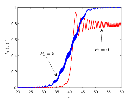
Figure 1: The numerical solution of Eq. (3) for the population of mode $1$ versus time. The parameters are $N=2$, $P_{1}=0.5$, $P_{2}=100$ and $P_{3}=0$ (red) or $5$ (blue).

III $N=2$ Case

We write Eq. (6) explicitly for $N=2$:

$$i\frac{d}{d\tau}\left(\begin{array}[]{c}b_{0}\\ b_{1}\end{array}\right)=\left(\begin{array}[]{cc}P_{3}\left|b_{0}\right|^{2}&-P_{1}\\ -P_{1}&P_{3}\left|b_{1}\right|^{2}-\tau+\omega_{1}\end{array}\right)\left(\begin{array}[]{c}b_{0}\\ b_{1}\end{array}\right).$$ (7)

As mentioned in Sec. II the couplings $b_{0}\leftrightarrow b_{-1}$ and $b_{1}\leftrightarrow b_{2}$ in Eq. (6) are nonresonant, and thus neglected in Eq. (7).

In the linear case, $P_{3}=0$, Eq. (7) takes the well-known LZ form LZ1 ; LZ2 with an avoided energy crossing at $\tau_{c}=\omega_{1}$ SideNote2 . If one starts in the ground state, $\left|b_{0}\left(\tau=0\right)\right|=1,$ the fraction of the population transferred to mode $1$ is given by the LZ formula $\left|b_{1}\left(\tau\gg\tau_{c}\right)\right|^{2}=1-\exp\left(-2\pi P_{1}^{2}\right)$ LZ1 ; LZ2 . The red curve in Fig. 1 shows an example for such LZ dynamics for $P_{1}=0.5$ and $P_{2}=100$. One can see a rapid population transfer around $\tau_{c}\approx 40.5$ converging to the value given by the LZ formula. However, when the explicit Kerr-type nonlinearity is introduced, the dynamics changes significantly. This is shown by the blue curve of Fig. 1, where $P_{3}=5$, whereas all other parameters are the same. In this case, the population transfer is much slower and almost linear in time reaching a higher final state for the same driving parameter $P_{1}$.

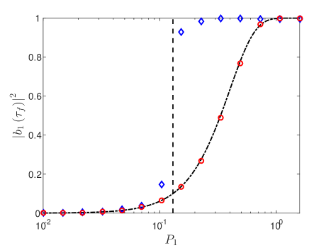
Figure 2: The numerical solution of Eq. (3) for the final population of mode $1$ as function of $P_{1}$. The parameters are $N=2$, $P_{2}=\tau_{f}=100$ and $P_{3}=0$ (red circles) or $5$ (blue diamonds). The dashed vertical line shows the theoretical NLZ threshold [Eq. 8], whereas the dashed-dotted curve is the theoretical LZ formula.

Figure 2 shows the final population of mode $1$ at $\tau_{f}=100$ as a function of $P_{1}$ and further demonstrates the differences between the two scenarios. In the linear $P_{3}=0$ case (red circles), the population transfer follows the LZ formula (dashed-dotted curve), whereas for $P_{3}=5$ (blue diamonds) the population of mode $2$ ”jumps” abruptly, reaching nearly full population transfer at lower driving strengths than in the linear case. This so-called nonlinear Landau-Zener transition (NLZ) was studied in the past in various contexts Batalov ; ChirpLazarSegev ; NLZ1 ; NLZ2 ; NLZ3 . It was shown that the growth of the population of mode $2$ is in fact linear in time (with superimposed oscillations), as illustrated in Fig. 1, and a nearly full population transfer takes place if $P_{1}$ exceeds a sharp threshold NLZ1 ; ChirpLazarSegev ; Batalov :

$$P_{1,cr}^{NLZ}\approx 0.29/\sqrt{P_{3}}.$$ (8)

The value of $P_{1,cr}^{NLZ}$ is shown in Fig. 2 by vertical dashed line, in good agreement with the numerically observed ”jump” in the transfer of population.

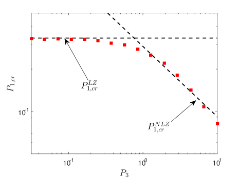
Figure 3: The solution of Eq. (3) for the threshold value $P_{1,cr}$ yielding transfer of one half of the population to mode $1$, as a function of $P_{3}$. The parameters are $N=2$, $P_{2}=\tau_{f}=200$, and the dashed lines show the theoretical predictions according to the LZ formula and Eq. (8). Numerical uncertainty is smaller than the marker sizes.

One can further demonstrate the differences between LZ and NLZ regimes by defining $P_{1,cr}$ as the value of $P_{1}$ for which half of the population transitions from mode $0$ to mode $1$. The numerically obtained value of $P_{1,cr}$ is plotted in Fig. 3 versus $P_{3}$. For large enough $P_{3}$, $P_{1,cr}$ matches $P_{1,cr}^{NLZ}$ (dashed diagonal line). However, in the LZ regime the LZ formula yields $P_{1,cr}^{LZ}=\sqrt{-\ln 0.5/2\pi}\approx 0.33$. And, indeed, for low $P_{3}$, $P_{1,cr}$ matches $P_{1,cr}^{LZ}$ (dashed horizontal line). The intersection of the two threshold values $P_{1,cr}^{NLZ}=P_{1,cr}^{LZ}$ yields a good estimate for the value of $P_{3}$ for which the transition between the two regimes takes place.

Our driving perturbation differs from that assumed in the asymptotic theories of LZ and NLZ processes because it involves a finite driving time prior to the energy crossing at $\tau_{c}$. Nevertheless, it will be assumed that $\tau_{c}$ is large enough for the two theories to be valid, which can always be accomplished by increasing $P_{2}$ (as $\tau_{c}\propto P_{2}$). Nevertheless, the breaking of this assumption is important in studying the $N\gg 1$ case in Sec. IV and, thus, requires a further discussion. For $\tau_{c}$ to be large enough for the applicability of the asymptotic LZ and NLZ theories, it must be larger than the characteristic time of population transfer from one mode to the next. In the case of LZ, the transition time $\Delta\tau_{LZ}$ is of order $O(1)$ when $P_{1}$ is small and $O(P_{1})$ when it is large, therefore we estimate $\Delta\tau_{LZ}=1+P_{1}$ LZtimescales . In the case of NLZ the estimate is $\Delta\tau_{NLZ}=2P_{3}$ Batalov . These two times can be combined into a single estimate for the transition duration

$$\Delta\tau=1+P_{1}+2P_{3}$$ (9)

and, therefore, $\tau_{c}\gg\Delta\tau$ guarantees that the dynamics is of the asymptotic LZ or NLZ type. Furthermore, since the neglected terms in the derivation of Eq. (6) and Eq. (7) oscillate with frequency proportional to $P_{2}$, the aforementioned condition also justifies the RWA approximation.

IV Quantum and Classical Effects for Large $N$

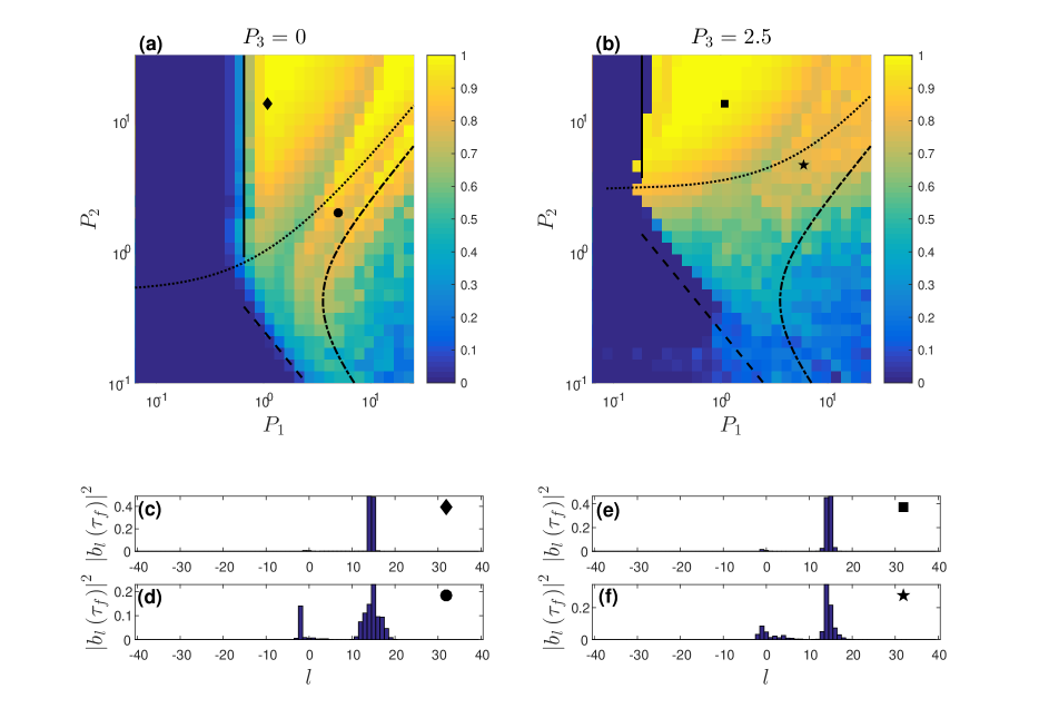
Figure 4: Color coded excitation efficiencies (see the text) in the $P_{1,2}$ parameter space for (a) $P_{3}=0$ and (b) $2.5$, as obtained from the numerical solution of Eq. (3), with $N=80$ and $\tau_{f}=\tau_{15}\approx 23.1P_{2}$. The lines represent different borderlines in the parameter space - The efficient LC threshold (solid line), efficient AR threshold (dashed line), quantum-classical separation (dotted line), and the large separatrix boundary (dashed-dotted line). Panels (c)-(f) show the population of each mode at $\tau_{f}$ for $P_{1,2}$ values shown by the corresponding markers in panels (a) and (b). For clarity, modes with $l>N/2$ are shifted and presented as $l<0$.

The controlled excitation in our system is not limited to the $N=2$ case, therefore the $N\gg 1$ limit is considered next (for some remarks on the case of moderate $N$ see App. B). Panels (c)-(e) in Fig. 4 show histograms of the final populations $\left|b_{l}\left(\tau_{f}\right)\right|^{2}$ for $N=80$ and $\tau_{f}\approx 23.1P_{2}$. The parameters $P_{1,2}$ in these panels correspond to those shown by corresponding markers in the parameter space of panels (a) and (b) , where $P_{3}=0$ and $2.5$, respectively. These figures illustrate a controlled transfer of the populations to the vicinity of a target mode (in this case, $l\approx 15$), with some width around this mode. In this section we show how the different parameters in the problem control the target mode, the fraction of the excited population, and the width of the excited distribution of modes.

IV.1 Quantum-mechanical ladder climbing

Panels (c) and (e) in Fig. 4 exhibit very narrow distributions (1 to 2 modes) and hint at the connection between the cases of $N=2$ and $N\gg 1$. This connection becomes apparent when one examines only two mode interaction $l-1\leftrightarrow l$ and neglects other modes in Eq. (6), i.e. solves

$$i\frac{d}{d\tau}\left(\begin{array}[]{c}b_{l-1}\\ b_{l}\end{array}\right)=\left(\begin{array}[]{cc}\Gamma_{l-1}&-P_{1}\\ -P_{1}&\Gamma_{l}\end{array}\right)\left(\begin{array}[]{c}b_{l-1}\\ b_{l}\end{array}\right),$$ (10)

where $\Gamma_{l}=P_{3}\left|b_{l}\right|^{2}-l\tau+\omega_{l}$. Similar to the case of $N=2$, Eq. (10) takes the form of LZ or NLZ transition, depending on the value $P_{3}$. However, in this case, there are many such transitions (resonances) and their timing is $l$ dependent. This temporal separation between the transitions allows the system to successively perform quantum energy LC via pairwise LZ or NLZ transitions. The time $\tau_{l}$ of the transition $l-1\leftrightarrow l$ can be found by equating $\Gamma_{l-1}=\Gamma_{l}$ (energy crossing) which yields

$$\tau_{l}=\frac{P_{2}N^{2}}{\pi^{2}}\sin\left({\frac{\pi}{N}}\right)\sin\left(\frac{\pi\left[2l-1\right]}{N}\right).$$ (11)

Examining Eq. (11), one can identify a resonant pathway of consecutive transitions from the ground state to $l\approx N/4$. The final driving time $\tau_{f}$ dictates how high in $l$ the system will climb and sets the target mode for the process. In the simulations of Fig. 4, $\tau_{f}\approx 23.1P_{2}$ so that $\tau_{f}=\tau_{15}$, as could be observed in panels (c)-(f). If the consecutive transitions are well separated in time, one can treat them as individual LZ or NLZ transitions, and use all of the results discussed in Sec. III for $N=2$. Specifically, the probability of population transfer will follow the LZ formula and will exhibit a sharp threshold on $P_{1}$ for the NLZ transition. Thus, the excitation efficiency (the fraction of the excited population) in the two cases should exhibit different characteristics. Once again, one can define $\overline{P}_{1,cr}$ as the value of $P_{1}$, which will drive $50\%$ of the population after $r$ transitions. Using the LZ formula one can calculate

$$\overline{P}_{1,cr}^{LZ}=\sqrt{-\frac{\ln\left(1-2^{-1/r}\right)}{2\pi}}.$$ (12)

For NLZ transitions, the sharp threshold guarantees that if the first transition was efficient, it will continue to be efficient later and, thus,

$$\overline{P}_{1,cr}^{NLZ}=P_{1,cr}^{NLZ}.$$ (13)

To check this prediction, Eq. (3) was solved numerically with $N=80$. The excitation efficiency was defined as the total population between modes $10$ and $20$ (upper half of the resonantly accessible modes). These results are color coded in panels (a) and (b) of Fig. 4. The population undergoes $r=10$ transitions between the ground state and the measurement window, and the corresponding $P_{1,cr}$ according to Eqs. (12), and (13) is plotted as vertical solid lines in panels (a) and (b). One can see that for large enough $P_{2}$, the excitation efficiency grows as expected with $P_{1}$: it significantly increases in the vicinity of $P_{1,cr}$, and grows sharply in the NLZ case [panel (b)].

The agreement with the numerics for high enough $P_{2}$ only is expected, as the assumption that different transitions are well separated in time, is not valid for small $P_{2}$. Using the logic of Sec. III, for the transitions to be well separated, one must require the typical time between the transitions to be larger than the typical duration of a single transition, as given by Eq. (9). In the limit $N\gg 1$, $l\ll N$, Eq. (11) shows that the time between two successive transitions is $2P_{2}$ (regardless of the value of $P_{3}$, since the temporal separation is set by the linear unperturbed problem $P_{1}=P_{3}=0$) and, therefore,

$$P_{2}\gg\frac{1}{2}+\frac{P_{1}}{2}+P_{3},$$ (14)

is the criterion for the LC. The line in the $P_{1,2}$ space on which the two sides of inequality (14) are equal is shown by the dotted lines in panels (a) and (b) of Fig. 4. One can see that the LC prediction holds only above this line. Furthermore, panels (c) and (e) of Fig. 4 (corresponding to final simulation time and parameters in the LC regime) involve only two levels as expected from separated successive LZ transitions. A movie illustrating this dynamics at earlier times for the parameters of panel (c) is presented in the Supplemental Material SUP . The observed temporal separability of the transitions differs from the lack of separability in the context of counterdiabatic protocols CA1 .

It should be noted that, although initially the transitions are nearly evenly separated (similar to other LC systems Ex3 ; Ex5 ; LZtimescales ) as one approaches larger $l$, the transitions become more frequent. Condition (14) does not hold in this case, and the dynamics will cease to be of LC nature. However, as could be observed in Fig. 4 and will be discussed below, condition (14) is still sufficient in the context of excitation efficiency.

But what happens when criterion (14) is not met and the transitions are not well separated? Figure 4 shows that there could still be efficient excitation, but now many modes are coupled at a time. This mixing of many different modes leads to classical-like behavior. This is also hinted by the wide distributions observed in panels (d) and (f), where the parameters are outside the LC regime. The semiclassical analysis of this regime will be our next goal.

IV.2 Semiclassical autoresonant regime

For studying the semiclassical evolution of the system when condition (14) is not met, return to Eq. (3) and assume that this set can be replaced by a continuous equation in the limit $N\gg 1$. Then one expands

$$\psi^{n\pm 1}=\sum_{j=0}^{\infty}\frac{1}{j!}\frac{d^{j}\psi^{n}}{dn^{j}}\left(\pm 1\right)^{j},$$

inserts this expansion into Eq. (3) and defines the continuous space-like variable $x\equiv n$ to get

$$i\frac{\partial\psi}{\partial\tau}+P_{2}\frac{N^{2}}{2\pi^{2}}\sum_{j=1}^{\infty}\frac{1}{\left(2j\right)!}\frac{\partial^{2j}\psi}{\partial x^{2j}}+(NP_{3}\left|\psi\right|^{2}+2P_{1}\cos\Phi)\psi=0.$$ (15)

Here, $\psi=\psi\left(x,\tau\right)$ and $\Phi=k_{0}x-\theta_{d}$ with $k_{0}=2\pi/N$. At this point, one writes the wave-like eikonal ansatz $\psi=b\left(x,\tau\right)\exp\left[iS\left(x,\tau\right)\right]$ Tracy , where $S$ is viewed as a rapidly oscillating phase variable, whereas $b$ is a slow amplitude. In addition, it is assumed that the derivatives of the fast phase

$$k \equiv \frac{\partial S}{\partial x},$$

$$\Omega \equiv -\frac{\partial S}{\partial\tau}$$

are both slow. The slowness in our problem means $|\partial(\ln G)/\partial x|\ll k$, where $G$ is any of the slow variables above Tracy . The eikonal ansatz models our basis modes $\Psi_{n}^{m}$ in discrete formalism. For example, the increase in $k$ in time would describe a transition to higher modes. Next, one approximates $\frac{d^{2j}\psi}{dx^{2j}}\approx be^{iS}\left(ik\right)^{2j}$ (neglecting small derivatives of $b$ and $k$), inserts this approximation into Eq. (15) and identifies the sum over $j$ as the Taylor expansion of $-2\sin^{2}\left(k/2\right)$ to obtain

$$i\frac{db}{d\tau}+b\Omega-P_{2}\frac{N^{2}}{\pi^{2}}b\sin^{2}\frac{k}{2}+(NP_{3}b^{2}+2P_{1}\cos{\Phi)}b=0.$$ (16)

The imaginary part of Eq. (16) yields $\frac{db}{d\tau}=0$. For a more accurate description of the evolution of the amplitude $b$ in the eikonal ansatz, one must go to a higher order of the approximation. However, it can be shown that the essentials of the resonant dynamics can be revealed without resolving $b$. We start with the case $P_{3}=0$ for which the real part of Eq. (16) reads

$$\Omega\left(x,\tau\right)=P_{2}\frac{N^{2}}{\pi^{2}}\sin^{2}\frac{k\left(x,\tau\right)}{2}-2P_{1}\cos{\Phi}.$$ (17)

Equation (17) is a first order partial differential equation for the phase variable $S$ in the eikonal ansatz, and can be solved along characteristics (rays). To this end, Eq. (17) can be interpreted as defining the function of three variables $\Omega=\Omega\left(x,k,\tau\right),$ where $k$ is also a function of $x,t$ and introduce the characteristics via

$$\frac{dx}{d\tau}=\frac{\partial\Omega\left(x,k,\tau\right)}{\partial k}.$$ (18)

Note that by construction,

$$\frac{d\Omega}{dx}+\frac{\partial k}{\partial\tau}=0,$$

which can be rewritten as

$$\frac{\partial\Omega}{\partial x}+\frac{\partial\Omega}{\partial k}\frac{\partial k}{\partial x}+\frac{\partial k}{\partial\tau}=0.$$

This yields the second ray equation

$$\frac{dk}{d\tau}=\frac{\partial k}{\partial\tau}+\frac{dx}{d\tau}\frac{\partial k}{\partial x}=-\frac{\partial\Omega}{\partial x},$$ (19)

which, in combination with (18), provides a complete system for following $x$ and $k~{}$along the rays. Note that these two equations comprise a Hamiltonian set with $\Omega\left(x,k,\tau\right)$ being the Hamiltonian. In addition,

$$\frac{d\Omega}{d\tau}=\frac{\partial\Omega}{\partial\tau}$$ (20)

and

$$\frac{dS}{d\tau}=\frac{\partial S}{\partial\tau}+\frac{\partial S}{\partial x}\frac{dx}{d\tau}=-\Omega+k\frac{\partial\Omega}{\partial k}.$$ (21)

Equations (18)-(21) can be conveniently solved to provide the phase factor $S$ as well as $x,k$, and $\Omega$ along the rays, provided the initial condition $S(x,\tau=0)$ is known on some interval of $x$. This knowledge also yields the initial conditions $k(x,\tau=0)$ and $\Omega(x,\tau=0)$ [from (17)] on this interval and solving the system (18)-(21) by starting on the interval allows to evolve the system in time. However, analyzing the phase-space of our Hamiltonian set is just as informative as shown below.

We insert Eq. (17) into Eqs. (18) and (19) and recall that $\Phi=k_{0}x-\tau^{2}/2$ to get

$$\frac{d\Phi}{d\tau} = P_{2}\frac{N}{\pi}\sin k-\tau,$$ (22)

$$\frac{dk}{d\tau} = -P_{1}\frac{4\pi}{N}\sin\Phi.$$ (23)

This system has the form known from many other classical autoresonantly driven systems studied in the past (e.g. Refs. Ex5 ; PhaseSpace ), so previously known results can be used directly in our case and we briefly describe these results. The angle $\Phi$ acts as a phase-mismatch between the driving force and the system. When the resonance condition $\frac{d\Phi}{d\tau}\approx 0$ is met continuously, $P_{2}\frac{N}{\pi}\sin k$ follows the driving frequency ($\omega_{d}=\tau$), thus the system is driven to higher modes. It should be noted that this resonance condition is identical to that given by Eq. (11) in the limit $N,l\gg 1$. Next, we take the second derivative of (22) and insert (23) to get

$$\frac{d^{2}\Phi}{d\tau^{2}}=-4P_{1}P_{2}\cos k\sin\Phi-1.$$ (24)

Here, we approximate $k\approx k_{r}$, where $k_{r}\left(\tau\right)$ is the value of $k$ satisfying the exact resonance condition Ex5 ; PhaseSpace . Then, Eq. (24) describes a pendulum with a time varying frequency and under the action of a constant torque. If $4P_{1}P_{2}\cos k_{r}>1$, the phase-space of the system has both open and closed trajectories. On the open trajectories, $\Phi$ grows indefinitely and $\sin k$ does not follow the driving frequency. In contrast on the closed trajectories, $\Phi$ and $d\Phi/d\tau$ are bounded and yield sustained phase-locking (autoresonance) of the system to the drive, i.e., a continuing excitation of $k$. The separatrix is the trajectory separating the closed and open trajectories in phase-space, and it only exists if $4P_{1}P_{2}\cos k_{r}>1$. Therefore, if one takes $\cos k_{r}$ at its maximal value of $1$, one obtains the threshold

$$P_{1}P_{2}=\frac{1}{4},$$ (25)

below which no autoresonant excitation is possible. This threshold is shown by the diagonal dashed lines in panels (a) and (b) in Fig. 4, showing good agreement with the numerical simulations for both values of $P_{3}$ SideNote3 , even though we have assumed $P_{3}=0$ above. This can be explained by observing that when $P_{3}\neq 0$, only Eq. (23) is affected and becomes

$$\frac{dk}{d\tau}=-P_{1}\frac{4\pi}{N}\sin\Phi+NP_{3}\frac{\partial\left(b^{2}\right)}{\partial x}.$$ (26)

Initially, in our simulations the additional term in Eq. (26) vanishes since $b$ is independent of $x$. Therefore, initially, the existence of the separatrix is not affected by $P_{3}$. At later times, if the separatrix exists, the focusing nonlinearity narrows the distribution and, thus, doesn’t scatter the trapped trajectories out of the separatrix. Numerically, the narrowing of the distribution is seen when comparing panels (d) and (f) in Fig. 4. Hence, the initial separatrix governs the existence of trapped trajectories, and since it is independent of $P_{3}$, threshold (25) describes the case $P_{3}\neq 0$ as well.

Until now, we have treated the trajectories inside the separatrix as those which will be excited to large $k$, but this is not the case when the separatrix becomes too large. In this case, even when a significant portion of the population is inside the separatrix, not all of it will be excited to large $k$, and subsequently will be precluded from our numerical measurement. The dashed-dotted line in panels (a) and (b) of Fig. 4 marks the values of $P_{1,2}$ for which the separatrix extends in $k$ at $\tau_{f}$ below our measurement window ($\pi/4$). Below this line the excitation efficiency drops, as more population ends up outside the measurement window. The aforementioned narrowing of the autoresonant bunch hinders this argument for $P_{3}\neq 0$, but nevertheless, for the values of $P_{3}$ in our simulations, this criterion still qualitatively agrees with the numerical simulations. The details of the separatrix related calculations are described in Appendix C.

Finally, we return to the quantum-classical separation line given by Eq. (14), which was derived under the assumption of equidistant energy crossings. Although this assumption breaks when the population is transferred to higher modes and several modes are coupled simultaneously, one can again use the semiclassical arguments as above. The same logic dictates that the excited population will undergo a dynamical transition from LC type evolution to AR evolution. This is guaranteed by the population being in resonance (again, one should note the similarities between the quantum and the classical resonance conditions), whereas the parameters in the efficient LC regime are always sufficient for efficient AR.

It should be noted that some features in panels (a) and (b) of Fig. 4 could not be accounted for using the theoretical framework described in this section. For example, the efficiency ”dip” close to the quantum-classical separation line (dotted line in the figure) could not be explored using the LC or AR arguments, as both approximations fail in this area of the parameter space. Furthermore, using the semi-classical theory to calculate the expected efficiency in the AR regime of the parameter space is beyond the scope of this paper. The main obstacle is the determination of the proper distribution of initial conditions for Eqs. (22) and (23). In a different context this calculation was possible when the system’s initial condition was a thermal state rather than the ground state Ex5 .

V Summary

In conclusion, we have studied the problem of the resonantly driven discrete (periodic over $N$ sites) nonlinear Schrodinger equation for a ground state initial condition. Based on four characteristic time scales in the problem, we introduced three dimensionless parameters $P_{1-3}$ characterizing the driving strength, the dispersion nonlinearity, and the Kerr-type nonlinearity, respectively and analyzed their effects on the resonant evolution. First, we analyzed the case of $N=2$ and used it to illustrate and analyze the processes of linear ($P_{3}=0$) and nonlinear ($P_{3}>0$) Landau-Zener transitions. We have used this two-level description in generalizing to the case of $N\gg 1$ and showed how successive linear or nonlinear Landau-Zener transitions, or LC, can occur in some regions of the three parameters space. Finally, we used semiclassical arguments to show how in a different region of the parameters space, when the transitions are not well separated and many modes are mixed, the classical-like AR evolution could appear. Our analysis identified the key borderlines in the parameter space, including the LC-AR separation line and the thresholds for effective LC or AR evolution.

The explicit Kerr-type nonlinearity introduces several new effects. First, a single nonlinear Landau-Zener transition is longer than the linear counterpart, and presents a sharp threshold with respect to the driving strength for achieving a full population transfer. As a result, in the case of $N\gg 1$, the LC regime is moved to higher-$P_{2}$ values in the $P_{1,2}$ parameter space. Furthermore, the effective LC threshold becomes sharp and is moved to lower-$P_{1}$ values in the parameter space. However, the efficient AR threshold remains the same and only the width of the autoresonant wavepacket narrows.

The two resonant mechanisms available in the DNLSE allow for intricate control, manipulation, and excitation of the system, and one can efficiently excite either a narrow (via LC) or a broad (via AR) distribution around given target modes. Our analysis was not limited to the case of periodic boundary conditions. The discussion of similar effects in the DNLSE with zero boundary conditions was presented in Appendix A. Furthermore, we expect that by adjusting the parameters of the problem both temporally and spatially, one can use the resonant mechanisms studied here to manipulate the system in the configuration space. In the context of optical waveguide arrays some of these effects were illustrated previously by spatially chirping the refractive index of each waveguide ChirpLazarSegev .

Owing to the versatility of the resonant mechanisms, their appearance for various initial and boundary conditions, and the relevance of the DNLSE to many experimental systems (particularly in the field of atomic physics and optics), this paper may open many new possibilities for future research. It would be also interesting to explore counterdiabatic schemes CA1 ; CA2 in this system.

Appendix A Zero Boundary Conditions

The resonant mechanisms discussed in this paper are not limited to the setting described in Sec. II. As an important additional demonstration, we will now show how the driven DNLSE with zero boundary conditions exhibits the same resonant characteristics. To perform this, we return to Eq. (1), but now imposing $\psi_{0}=\psi_{N-1}=0$ at all times (reducing the system to $N-2$ degrees of freedom) and using a modified standing wave-type chirped driving:

$$\begin{array}[]{ll}i\frac{d\psi_{n}}{dt}&+\frac{1}{\Delta^{2}}\left(\psi_{n+1}+\psi_{n-1}-2\psi_{n}\right)\\ &+\left[\beta\left|\psi_{n}\right|^{2}+\varepsilon\cos\theta_{d}\cos\left(\frac{\pi n}{N-1}\right)\right]\psi_{n}=0.\end{array}$$ (27)

To replicate the analysis of Sec. III, the new basis functions are the standing wave solutions of the linearized, unperturbed ($\beta,\varepsilon=0$) equation:

$$\Psi_{n}^{m} = \sqrt{\frac{2}{N-1}}e^{-iw_{m}t}\sin\left(k_{m}n\right),$$

$$k_{m} = \frac{\pi m}{N-1},$$

$$w_{m} = \frac{4}{\Delta^{2}}\sin^{2}\left(k_{m}/2\right),$$

$$m = 1,2,...,N-2.$$

The fact that the dispersion remains the same for both types of boundary conditions is important in exhibiting the same resonant characteristics. It is possible to define the parameters $P_{1-3}$ in much the same way as in Sec. II, but we refrain from this to avoid excessive notations at this point. We continue, following Sec. II, to finding the corresponding DNLSE for coefficients $a_{m}$ in the expansion $\psi_{n}=\sum_{m}a_{m}\Psi_{n}^{m}$. Inserting this expansion into Eq. (27), multiplying by ${\Psi_{n}^{l}}^{\ast}$ and summing over $n$ we get

$$\begin{array}[]{ll}i\frac{da_{l}}{dt}&+\frac{\varepsilon}{2}\cos\theta_{d}\left[a_{l-1}e^{i\Delta w_{l}t}+a_{l+1}e^{-i\Delta w_{l+1}t}\right]\\ &+\frac{\beta}{2\left(N-1\right)}\left[-A_{1}^{1}+A_{-1}^{1}+A_{1}^{-1}-A_{-1}^{-1}\right]=0,\end{array}$$ (28)

where

$$A_{j}^{k}=\sum_{m^{\prime},m^{\prime\prime}}a_{l+jm^{\prime}+km^{\prime\prime}}a_{m^{\prime}}^{\ast}a_{m^{\prime\prime}}e^{-i\left(w_{l+jm^{\prime}+km^{\prime\prime}}-w_{m^{\prime}}+w_{m^{\prime\prime}}-w_{l}\right)t}.$$

Now, we employ the RWA to get

$$-A_{1}^{1}+A_{-1}^{1}+A_{1}^{-1}-A_{-1}^{-1}\approx 3a_{l}-a_{l}\left|a_{l}\right|^{2},$$

and

$$\cos\theta_{d}\approx\frac{1}{2}e^{-i\theta_{d}},$$

for the resonant pathway ascending from mode $0$. Finally, the transformation to the rotating frame of reference $b_{l}=a_{l}\exp\left(il\theta_{d}-iw_{l}t-i3t\right)$ yields

$$i\frac{db_{l}}{dt}=-b_{l}\left(l\frac{d\theta_{d}}{dt}-w_{l}\right)+\frac{\beta}{2\left(N-1\right)}\left|b_{l}\right|^{2}b_{l}-\frac{\varepsilon}{4}\left(b_{l-1}+b_{l+1}\right),$$ (29)

which has the same form as Eq. (6). Therefore, the system with zero boundary conditions could be controlled and excited in the same way as the system with periodic boundary conditions. Note that in this case there is no coupling between modes $1$ and $N-2$, removing some of the subtleties encountered in the original problem.

Appendix B Moderate $N$ Case

For moderate $N,$ the semiclassical description is not valid, but one can still induce a ladder-climbing type behavior. However, unlike the case of $N\gg 1$, now the exact structure of the resonant ladder plays a more significant role. For example, if $N$ is divisible by $4$ the last two transitions in the resonant pathway will occur simultaneously resulting in a three level LZ transition (sometimes referred to as a ”bow tie” transition) 3LZA ; 3LZB ; 3LZC . In this case, the efficiency of this double transition is given by $\left(1-\exp\left[-\pi P_{1}^{2}\right]\right)^{2}$ 3LZB . This effect could only (realistically) be observed for moderate $N$, as for the $N\gg 1$ case, the system will already behave classically when this final transition is reached.

Although there is no semi-classical dynamics in this case, the separation line of the form (14) is still useful in demonstrating when the system could undergo the full ladder-climbing process from mode $0$ to the maximal accessible mode $l_{max}=D+1$ ($D\$being $N/4$ rounded down to the nearest integer). As in Sec. IV, we must demand that the minimal time between transitions is longer than the duration of a single transition as given by Eq. (9). One can show that this minimal time is either the time of the first transition $\tau_{1}$ when $N\leq 4$, or the time between the two last transitions when $N>4$. The time between the two last transitions is $\tau_{l_{max}}-\tau_{l_{max}-1}$ (when $N$ is not divisible by $4$) or $\tau_{l_{max}-1}-\tau_{l_{max}-2}$ (when $N$ is divisible by $4$).

Appendix C Separatrix Related Calculations

As discussed in Sec. IV, if the separatrix becomes too large, one can not distinguish between the captured and the not captured into resonance trajectories, as the captured trajectories might end up outside the numerical measurement window. To analyze this effect, one must examine the size of the separatrix. We begin by writing the Hamiltonian associated with Eq. (24),

$$H\left(\Phi,\frac{d\Phi}{d\tau}\right)=\frac{1}{2}\left(\frac{d\Phi}{d\tau}\right)^{2}-4\cos k_{r}P_{1}P_{2}\cos\Phi+\Phi,$$ (30)

where the resonance condition (22) yields $\cos k_{r}=\sqrt{1-\left(\frac{\pi\tau}{P_{2}N}\right)^{2}}$. The separatrix is the trajectory for which $H$ equals the value of the potential at its maximum point. Inserting this value of $H$ into (30) and shifting $\Phi$ such that $\Phi=0$ at the maximum point of the potential, we find the equation for the separatrix:

$$\left.\frac{d\Phi}{d\tau}\right|_{sep}^{\pm}=\pm 2^{1/2}\sqrt{B\left(1-\cos\Phi\right)+\sin\Phi-\Phi},$$ (31)

where $B=\sqrt{\left(4\cos k_{r}P_{1}P_{2}\right)^{2}-1}$. Following the arguments in Sec. IV, we demand that the lower end of the separatrix in $k,\Phi$ phase-space at the final driving time is higher than the lower end of our measurement window located at $k=\pi/4$. Thus, we invert Eq. (22) and insert (31) to get the condition

$$\arcsin\left[\left(\left.\frac{d\Phi}{d\tau}\right|_{sep}^{-}+\tau_{f}\right)\frac{\pi}{P_{2}N}\right]>\frac{\pi}{4}.$$ (32)

The dashed-dotted line in Fig. 4 is calculated numerically based on the limiting case of (32).

References

- (1) A.S. Davydov, J. Theor. Bio. 38, 559 (1973).
- (2) P.G. Kevrekidis and R. Carretero-Gonzalez, The discrete nonlinear Schrodinger equation : mathematical analysis numerical computations and physical perspectives (Springer, Berlin, 2009).
- (3) H.S. Eisenberg, Y. Silberberg, R. Morandotti, A.R. Boyd, and J.S. Aitchison, Phys. Rev. Lett. 81, 3383 (1998).
- (4) E. Smirnov, C.E. Ruter, M. Stepic , D. Kip, and V. Shandarov, Phys. Rev. E 74, 065601(R) (2006).
- (5) R. Morandotti, U. Peschel, J.S. Aitchison, H.S. Eisenberg, and Y. Silberberg, Phys. Rev. Lett. 83, 4756 (1999).
- (6) Y. Lahini, A. Avidan, F. Pozzi, M. Sorel, R. Morandotti, D.N. Christodoulides, and Y. Silberberg Phys. Rev. Lett. 100, 013906 (2008).
- (7) B.P. Anderson and M.A. Kasevich, Science 282, 1686 (1998).
- (8) A. Smerzi, A. Trombettoni, P.G. Kevrekidis, and A.R. Bishop, Phys. Rev. Lett. 89, 170402 (2002).
- (9) F.S. Cataliotti, L. Fallani, F. Ferlaino, C. Fort, P. Maddaloni, and M. Inguscio, New J. Phys. 5, 71 (2003).
- (10) M. Greiner, O. Mandel, T. Esslinger, T.W. Hnsch and I. Bloch, Nature 415, 39 (2002).
- (11) A. Zenesini, H. Lignier, D. Ciampini, O. Morsch, and E. Arimondo, Phys. Rev. Lett. 102, 100403 (2009).
- (12) H. Lignier, C. Sias, D. Ciampini, Y. Singh, A. Zenesini, O. Morsch, and E. Arimondo, Phys. Rev. Lett. 99, 220403 (2007).
- (13) D. Witthaut, E. M. Graefe, S. Wimberger, and H. J. Korsch, Phys. Rev. A 75, 013617 (2007).
- (14) A. Zenesini, C. Sias, H. Lignier, Y. Singh, D. Ciampini, O. Morsch, R. Mannella, E. Arimondo, A. Tomadin and S. Wimberger, New Journal of Physics 10, 053038 (2008).
- (15) B. Eiermann, Th. Anker, M. Albiez, M. Taglieber, P. Treutlein, K.P. Marzlin, and M.K. Oberthaler, Phys. Rev. Lett. 92, 230401 (2004).
- (16) A. Trombettoni and A. Smerzi, Phys. Rev. Lett. 86, 2353 (2001).
- (17) S. Chelkowski and G. N. Gibson, Phys. Rev. A 52, R3417 (1995).
- (18) D. J. Maas, D. I. Duncan, R. B. Vrijen, W. J. van der Zande, and L. D. Noordam, Chem. Phys. Lett. 290, 75 (1998).
- (19) G. Marcus, A. Zigler, and L. Friedland, Europhys. Lett. 74, 43 (2006).
- (20) G. Marcus, L. Friedland, and A. Zigler, Phys. Rev. A 69, 013407 (2004).
- (21) T. Armon and L. Friedland, Phys. Rev. A 96, 033411 (2017).
- (22) J. Fajans and L. Friedland, Am. J. Phys. 69, 1096 (2001).
- (23) Y. Shalibo, Y. Rofe, I. Barth, L. Friedland, R. Bialczack, J. M. Martinis, and N. Katz, Phys. Rev. Lett. 108, 037701 (2012).
- (24) I. Barth, I. Y. Dodin, and N. J. Fisch, Phys. Rev. Lett. 115, 075001 (2015).
- (25) K. Hara, I. Barth, E. Kaminski, I. Y. Dodin, and N. J. Fisch, Phys. Rev. E 95, 053212 (2017).
- (26) G. Manfredi, O. Morandi, L. Friedland, T. Jenke, and H. Abele, Phys. Rev. D 95, 025016 (2017).
- (27) S.V. Batalov, A.G. Shagalov, and L. Friedland, Phys. Rev. E 97, 032210 (2018).
- (28) L. D. Landau, Phys. Z. Sowjetunion 2, 46 (1932).
- (29) C. Zener, Proc. R. Soc. London, Ser. A 137, 696 (1932).
- (30) A. Barak, Y. Lamhot, L. Friedland, and M. Segev, Phys. Rev. Lett. 103, 123901 (2009).
- (31) R. Khomeriki, Phys. Rev. A 82, 013839 (2010).
- (32) G. Assanto, L.A. Cisneros, A.A. Minzoni, B.D. Skuse, N.F. Smyth, and A.L. Worthy, Phys. Rev. Lett. 104, 053903 (2010).
- (33) N. Tsukada, Phys. Rev. A 69, 043608 (2004).
- (34) When is even, the sum could vanish if or . However, in all of these cases, the resulting couplings link modes below and above . Since we use initial condition and the resonant pathway leads the population to higher modes, one of the modes in the coupling terms always vanishes, making the couplings irrelevant.
- (35) In this context, the nonresonant coupling neglected in Eq. (7) is associated with the second energy crossing occurring at , which the driver ”misses” by starting at . This peculiar effect could be seen numerically by starting the driver at well before , yielding a double transition - from mode to and back, as the drive sweeps through both energy crossings.
- (36) L. Friedland, Phys. Fluids B, 4, 3199 (1992).
- (37) O. Zobay and B.M. Garraway, Phys. Rev. A 61, 033603 (2000).
- (38) B. Wu and Q. Niu, Phys. Rev. A 61, 023402 (2000).
- (39) I. Barth, L. Friedland, O. Gat, and A.G. Shagalov, Phys. Rev.A 84, 013837 (2011).
- (40) See Supplemental Material at [LINK COMES HERE] for a short movie showing the evolution of the population with parameters identical to those of Fig. 4(c).
- (41) M. Theisen, F. Petiziol, S. Carretta, P. Santini, and S. Wimberger, Phys. Rev. A 96, 013431 (2017).
- (42) T. Armon and L. Friedland, Phys. Rev. A 93, 043406 (2016).
- (43) E.R. Tracy, A.J. Brizard, A.S. Richardson, and A.N. Kaufman, Ray tracing and beyond (Cambridge Univ Press, Cambridge UK, 2014).
- (44) The small excitation below the threshold is the result of non-resonant and non-adiabatic effects. Unlike other systems Ex5 ; PhaseSpace , the finite nature of the energy ladder makes it impossible to create separation between resonantly and non-resonantly excited populations.
- (45) F. Petiziol, B. Dive, F. Mintert, and S. Wimberger, Phys. Rev. A 98, 043436 (2018).
- (46) C.E. Carroll and F.T. Hioe, J. Phys. A: Math. Gen. 19, 1151 (1986).
- (47) C.E. Carroll and F.T. Hioe, J. Phys. A: Math. Gen. 19, 2061 (1986).
- (48) S. Brundobler and V. Elser, J. Phys. A: Math. Gen. 26, 1211 (1993).