Identification of Young Stellar Object candidates in the Gaia DR2 x AllWISE catalogue with machine learning methods

Abstract

The second Gaia Data Release (DR2) contains astrometric and photometric data for more than 1.6 billion objects with mean Gaia $G$ magnitude $<$20.7, including many Young Stellar Objects (YSOs) in different evolutionary stages. In order to explore the YSO population of the Milky Way, we combined the Gaia DR2 database with WISE and Planck measurements and made an all-sky probabilistic catalogue of YSOs using machine learning techniques, such as Support Vector Machines, Random Forests, or Neural Networks. Our input catalogue contains 103 million objects from the DR2xAllWISE cross-match table. We classified each object into four main classes: YSOs, extragalactic objects, main-sequence stars and evolved stars. At a 90% probability threshold we identified 1 129 295 YSO candidates. To demonstrate the quality and potential of our YSO catalogue, here we present two applications of it. (1) We explore the 3D structure of the Orion A star forming complex and show that the spatial distribution of the YSOs classified by our procedure is in agreement with recent results from the literature. (2) We use our catalogue to classify published Gaia Science Alerts. As Gaia measures the sources at multiple epochs, it can efficiently discover transient events, including sudden brightness changes of YSOs caused by dynamic processes of their circumstellar disk. However, in many cases the physical nature of the published alert sources are not known. A cross-check with our new catalogue shows that about 30% more of the published Gaia alerts can most likely be attributed to YSO activity. The catalogue can be also useful to identify YSOs among future Gaia alerts.

1 Introduction

Astronomy now is facing a major data avalanche. The analysis of huge amounts of data is a new challenge that researchers have to cope with. The term “data mining” is more and more widespread in the astronomical community. What is discovered with data mining and knowledge discovery in databases, can be further studied on a statistical basis. Already by April, 2019, more than 1 300 refereed papers are available via the NASA ADS database with titles including the phrase “machine learning” in various topics like galaxy cluster mass estimation (e.g. Armitage et al., 2019), exoplanet transit detection (e.g. Schanche et al., 2019), power spectra prediction from reionization simulations (e.g. Jennings et al., 2019) or morphological classification of 14 245 radio AGNs (e.g. Ma et al., 2019). Supervised and unsupervised machine learning techniques are available to deal with problems like clustering, classification, regression and outlier detection, and they can easily outperform traditional methods, e.g. star-galaxy separation on colour–brightness and colour–colour diagrams (e.g. Małek et al., 2013).

One important research area, where this new attitude will bring fundamental new results, is star formation. How the Sun – and in general, stars – were born, is identified as one of the top four areas of modern astronomy in the European Astronet Science Vision document. Star formation starts as the gravitational collapse of dense, rotating, magnetic molecular cloud cores. Due to angular momentum conservation, this process is always accompanied by the formation of circumstellar disks (e.g. Shu et al., 1987), sometimes still embedded in their envelope. Disk-bearing YSOs can be recognized by the infrared excess emission originating from the dusty component of these structures. Another signature of newly born stars with protoplanetary disks is their brightness variations that provide information on the transitions between protostellar evolutionary stages, on the structure of their circumstellar disks, and on the different ways that protostars may affect the initial conditions of planet formation (e.g. Ábrahám et al., 2009; Kóspál et al., 2012).

A long–standing problem of current star formation theories is the luminosity problem, meaning that the expected cloud core infall rates for Class I YSOs is the order of 10^-6 M_⊙ yr^-1, that should cause 10–100 times higher luminosity than observed (Kenyon et al., 1990; Enoch et al., 2009; Dunham et al., 2014). The other problem is that the Hertzsprung-Russel diagrams (HRD) of pre–main sequence (PMS) star clusters have a wide-scatter about the best–fitting isochrone. A possible single explanation for both these problems is episodic accretion (e.g. Aduard et al., 2014). The star normally collects material from the surrounding envelope and disk at a low rate ($10^{-7}\mathrm{M}_{\odot}\mathrm{yr}^{-1}$), and at rare occasions the accretion rate rapidly increases ($10^{-4}\mathrm{M}_{\odot}\mathrm{yr}^{-1}$). If most of the PMS stars show some eruptive behavior then the lower–than–expected luminosity is explained by the very low accretion rate which is happening for most of the time in this evolutionary phase. On the other hand the scatter would be the result of the more dramatic accretion events, which affects the locations of the stars in the HRD (e.g. Baraffe, Chabrier, & Gallardo, 2009).

Lucas et al. (2017) propose that low level variations of the accretion are interpreted as an effect of the stellar magnetosphere, generating multiple, often unstable accretion flows (e.g. Romanova, Kulkarni & Lovelace, 2008). More dramatic, significant eruptive events have been classically divided into two sub-classes (see e.g. Herbig, 1989): (1) FU Orionis-type variables (FUors) are thought to be the most dramatic examples of episodic accretion. FUors exhibit 5–6 mag optical outbursts attributed to highly enhanced accretion (Hartmann & Kenyon, 1996). During these outbursts, accretion rates from the circumstellar disk onto the star are on the order of 10^-4 M_☉yr^-1, three orders of magnitude higher than in quiescence. The exact physical mechanism of FUor outbursts is debated. Explanations include viscous-thermal instabilities in the disk (Bell & Lin, 1994), a combination of gravitational and magnetorotational instabilities (Armitage et al., 2001, MRI), or accretion of clumps in a gravitationally fragmenting disk (Vorobyov & Basu, 2005, 2006, 2015). Yet another type of theory involves a close stellar or substellar companion that perturbs the disk and triggers the onset of the enhanced accretion (Bonnell & Bastien, 1992; Lodato & Clarke, 2004; Nayakshin & Lodato, 2012). (2) As it is described by e.g. Kóspál et al. (2014), EX Lup-type objects (EXors) are a group of low-mass pre-main sequence stars, repetitively showing optical outbursts of $\sim$1–5 mag. The duration of these eruptive events covers timescales ranging from a few months to a few years. The outburst is usually attributed to enhanced accretion from the inner circumstellar disk (within $\sim$0.1 AU) to the stellar photosphere, caused by an instability in the disk (Herbig, 1977, 2008). In quiescence, EXors typically accrete at a rate of 10^-10 to 10^-7M_☉yr^-1, while in outburst, accretion rates are about an order of magnitude higher (Lorenzetti et al., 2012). These brief phenomena may significantly contribute to the build-up of the final stellar mass. Moreover, the outbursts have an effect on the circumstellar material, as well, as demonstrated by Ábrahám et al. (2009). They discovered episodic crystallization of silicate grains in the disk surface due to the increased luminosity and temperature during the 2008 outburst of EX Lup, resulting in material that forms the building blocks of primitive comets.

One way to resolve the above problems is if we become more efficient in identifying the eruptive phenomena of YSOs and we are able to monitor more of them with high temporal resolution, so more observational data for theories would be collected.

Variability in YSOs occurs on timescales spanning a wide range and time-domain observation of the sky is a rapidly developing field of research. Recent surveys, e.g. ASAS (Pojmanski, 1997) PTF (Law et al., 2009), YSOVAR (Morales-Calderón et al., 2011), CSI 2264 (Cody et al., 2014), ASAS-SN (Shappee et al., 2014; Kochanek et al., 2017) provided light curves of millions of sources.

Present and future observations involve at least an order of magnitude more, billions of sources, with hundreds of measured attributes per source. Gaia (Gaia Collaboration, 2016) is a currently operational cornerstone mission of the European Space Agency. The mission is not only the most ambitious stellar astrometric project ever, but also the best transient discovery machine today. It collects photometric observations of $\sim$1.6 billion stars down to an extreme faint limit of 20.7 mag in the $G$ band and obtains low-resolution spectroscopy down to $\sim$ 19 mag for an average of $\sim$80 epochs during the nominal five year mission, although the cadence is highly depending on the scanning law (Wyrzykowski et al., 2012). In the future, LSST (Iveziĉ et al., 2008) will produce 30 terabytes of data in one night and will detect stars brighter than 24.5 magnitude. The cadence of the LSST is planned to be 2–3 days (split between different filters).

Based on the Gaia data, stellar light curves with $\sim$30 days cadence can be constructed, and analysed for variability. The task of the Gaia Photometric Science Alerts System (operated by the Institute of Astronomy at Cambridge University) is to check all light curves, and search for unpredictable transients which may herald important astrophysical events, like stellar explosions. Currently $\sim$6 alerts per day are selected from about 10⁵–10⁶ candidates, and posted on a dedicated webpage a few days after the detection.

Up to now, more than 7 500 alerts were published, triggering follow-up observations and scientific papers (e.g. Hillenbrand et al., 2018). From this sample several thousands alerts were published as unknown type of object and only $\sim$120 were proposed to be variable YSOs by the alerts team. The latter number is astonishingly low, because decades of groundbased monitoring observations demonstrated that young stars also frequently exhibit spectacular variations, both brightenings and fadings. Since Gaia is the only all-sky transient survey today, a number of events would go unnoticed without the alerts. With a more efficient identification of YSOs among the alerted objects, Gaia could make a strong scientific contribution in the field of star and planet formation, by discovering and publishing otherwise unnoticed YSO brightenings and fadings.

In this paper we aim at identifying YSO candidates based on the second data release of the Gaia mission. Probability based classification of $\sim$103 million sources into four main object classes (Y – YSO candidates, EG – extragalactic sources, MS – main sequence stars, E – evolved stars) was done using multi-band photometric data. Section 2 describes the catalogues and maps we used in our study, also gives a brief summary of the different classification methods. In Section 3 we describe how effectively the different methods performed in our tests. In Section 4 we apply our YSO candidate selection to a star forming cloud and compare our results to that of a recently published study. We also cross-match our candidates with the published and unpublished Gaia alerts, analyse their flux asymmetry distribution and find that we can increase the number of YSO related alerts among the studied sample by 50%.

2 Data and methods

2.1 Catalogues and maps

2.1.1 Gaia DR2

The second release of the Gaia Data (DR2) was made available on 2018 April 25^th, consisting of astrometry and photometry for over 1.6 billion sources brighter than magnitude 20.7 in the $G$ band (Gaia Collaboration, 2018). Gaia DR2 is based on observations collected between 2014 July 25^th and 2016 May 23^rd. The main content of the catalogue and the limitations of the DR2 are well explained on the Gaia Cosmos Webpage and in Gaia Collaboration (2018).

For our science case it is important to note that while the DR2 catalogue is essentially complete between $G=12$ and $G=17$, it has an ill-defined faint magnitude limit, which depends on celestial position. YSOs, especially at the early stages of their evolution, not only emit the majority of their radiation at near- and mid-infrared wavelengths and are fainter in the part of the electromagnetic spectrum visible to $Gaia$, but being typically associated with dense clouds and accreting envelopes and disks they suffer larger extinctions than main sequence and evolved stars. Based on our training samples (see Section 2.3) we found that 55% of the YSOs detected by the $Spitzer$ Space Telescope (Werner et al., 2004) is present in the DR2 and 68% of those are brighter than 17 magnitudes in the $G$ band. Because of the scan law pattern, source density fluctuations also exist, which affect the completeness of crowded regions, like star forming regions. Crowding and blending are important features of star forming regions, and especially at fainter magnitudes ($G>19$) the photometric measurements from the blue and red photometers suffer from an insufficiently accurate background estimation and from the lack of specific treatment of blending and contamination from nearby sources.

2.1.2 AllWISE and 2MASS catalogue

WISE is a NASA space telescope that was launched in December 2009. It scanned the whole sky in four near– and mid–infrared passbands: $W1$, $W2$, $W3$ and $W4$, centered at at 3.4, 4.6, 12, and 23 $\mu$m, respectively. The AllWISE Source Catalogue (Cutri et al., 2013) was produced by combining the WISE single-exposure images from several survey phases and contains 747 634 026 sources. According to the explanatory supplement the angular resolution is 6$\arcsec$.1, 6$\arcsec$.4, 6$\arcsec$.5, and 12$\arcsec$.0, in bandpasses W1–W4 respectively, with 5$\sigma$ detection limit estimated to be 0.054, 0.071, 0.73, and 5 mJy.

The WISE telescope (Wright et al., 2010) was not designed for observation of faint and deeply embedded objects, but still provided the most recent all-sky survey in the part of the electromagnetic spectrum, where YSOs usually emit the bulk of their radiation.

The AllWISE catalogue already includes the $J$, $H$ and $K_{s}$ band photometric data from the 2MASS point- and extended source catalogues (Skrutskie et al., 2006).

2.1.3 Planck foreground map

YSOs are located predominantly in regions containing a large amount of dust. The Planck space telescope collected infrared light emitted by the dust particles for the all-sky. In order to decide if a source is associated with a dusty region we extracted dust opacity ($\tau$) value for each source. This value also gives us a clue about the volume of interstellar extinction which has a major impact on the colour of the sources. We used the 353 GHz R2.01 Planck dust opacity map (Planck Collaboration, 2016) value at the position of each object. The map is a HealPix image, with NSide=2048 and a pixel resolution of 1.718$\arcmin$.

2.2 Initial dataset

As explained in Section 1, the spectral energy distribution (SED) of YSOs with circumstellar disks show an infrared excess. Automated classifiers designed to identify disk bearing YSOs provide optimal performance if we include infrared data. Therefore, in this study we are only interested in those $Gaia$ DR2 objects which have matching detections in the AllWISE catalogue. The cross-match of the AllWISE and DR1 catalogues was done by Marrese et al. (2017). Their method accounts for the proper motion, different epochs and also e.g. the local surface density of the external catalogue. This exercise was repeated for the DR2 and the cross-matching table was part of the official data release (Marrese et al., 2018). For our case we used the AllWISE BestNeighbour table that contained 300 207 917 matches. The table listed the Gaia Source IDs and the AllWISE source IDs for all pairs.

As we are mostly interested in finding YSOs and YSO candidates, we explored only a subset of the Gaia DR2 X AllWISE table. To identify the regions where YSOs are mostly located, we checked the Planck dust opacity map (Section 2.1.3) values at the celestial positions of the known YSOs, collected from the SIMBAD database, the Spitzer archives and the literature (see Section 2.3 for more details). We found that 99% of the known YSOs are located in regions where the dust opacity value is higher than 1.3$\times 10^{-5}$.

The sources outside these regions, and those lacking data in one or more photometric bands were removed from our list. We also removed those objects where multiple $Gaia$ IDs were associated with one AllWISE object. As a result our initial dataset contained 101 838 724 sources including Gaia optical G magnitudes, $J$, $H$, $K_{s}$ magnitudes from 2MASS, AllWISE magnitudes, and the optical depth ($\tau$) from the Planck dust opacity map.

2.3 Training sample

Finding YSO candidates among unknown sources is a typical classification problem. We used supervised machine learning techniques to identify YSO candidates. For such algorithms training samples needs to be created. A training sample contains data of objects from known classes. The problem to be solved is to find the best algorithm and those properties (i.e. colours, source extension, environmental parameters) which describe the different classes in the most meaningful way and can separate the classes the most efficiently. The goal is to maximize the number of true positive (e.g. a known YSO is classified as YSO) and minimize the number of false negative classifications (when a YSO is classified as something different).

In our previous works we attempted to identify YSO candidates based on AKARI data combined with WISE photometry (Tóth et al., 2014) and on purely AllWISE data (Marton et al., 2016). In these attempts our training samples were based on the SIMBAD database. SIMBAD includes astronomical objects from scientific publications. It provides information on the nature of the objects via the main_type and other_type columns. The main_type column includes information on the most specific type of the object (if known), which is the primary object type, while the other_type lists the primary and the more generic types, e.g. the AllWISE source J173821.67-293459.5 has a “YSO” main_type, but the other_type is “Y*O|IR”. Still, in many cases the main_type is a general object type, like “Galaxy” or “Star”.

In this study we searched not only the SIMBAD, but also used $\sim$80 catalogues from the literature to identify the known YSOs and other object types in order to have the best possible training samples. All the objects were grouped into four object classes: Main-sequence stars (MS); Extragalactic objects (EG); Evolved stars (E); YSOs (Y). These classes were built from the following datasets and catalogues:

• Main-sequence stars (MS):

  • Main-sequence stars below 6500 K observed by the Kepler Space Telescope (McQuillan et al., 2014)

  • Main-sequence stars from the 3rd edition all-sky catalog of Kharchenko (2001)

  • Main-sequence stars from the Catalogue of stellar UV fluxes (Thompson et al., 1980)

• Extragalactic objects (EG):

  • SIMBAD main types equal to AGN, AGN_Candidate, BClG, BLLac, BLLac_Candidate, Blazar, Blazar_Candidate, BlueCompG, Compact_Gr_G, EmG, Galaxy, GinCl, GinGroup, GinPair, GravLensSystem, GroupG, HII_G, IG, LensedG, PairG, PartofG, QSO, QSO_Candidate, RadioG

  • Objects from the Allwise AGN Gaia DR2 cross-identification table

• Evolved stars (E)

  • SIMBAD main types of Mira, RGB*, post-AGB*, RRLyr, AGB* and HB*

  • Objects of the Gaia DR2 Cepheid stars table and RR Lyrae stars table

• YSOs (Y)

  • Photometric YSO catalogues found in the VizieR database (Appendix A)

  • Spectroscopic YSO catalogues listed by VizieR (Appendix B)

  • YSO related Spitzer publications (Appendix C)

  • Spitzer YSOs and YSO candidates from the project "From Molecular Cores to Planet-Forming Disks" (C2D) (Evans et al., 2003)

The objects of the above catalogues were cross-matched with our initial dataset (Section 2.2). In Figure 1 we show the distribution of the angular distance values between the Gaia DR2 positions and that of the Spitzer YSOs and YSO candidates. In 95% of those cases where a counterpart was found within 5^′′, the matching source was closer than 1^′′. We also checked the distances between the $Gaia$ DR2 and the AllWISE counterpart of these sources, listed in the $Gaia$ DR2 x AllWISE table and found that 99.7% of the best neighbours are within 1^′′. Thus, we decided to use a 1^′′ search radius in the procedure, although it is an arbitrary number, but it fits our requirements.

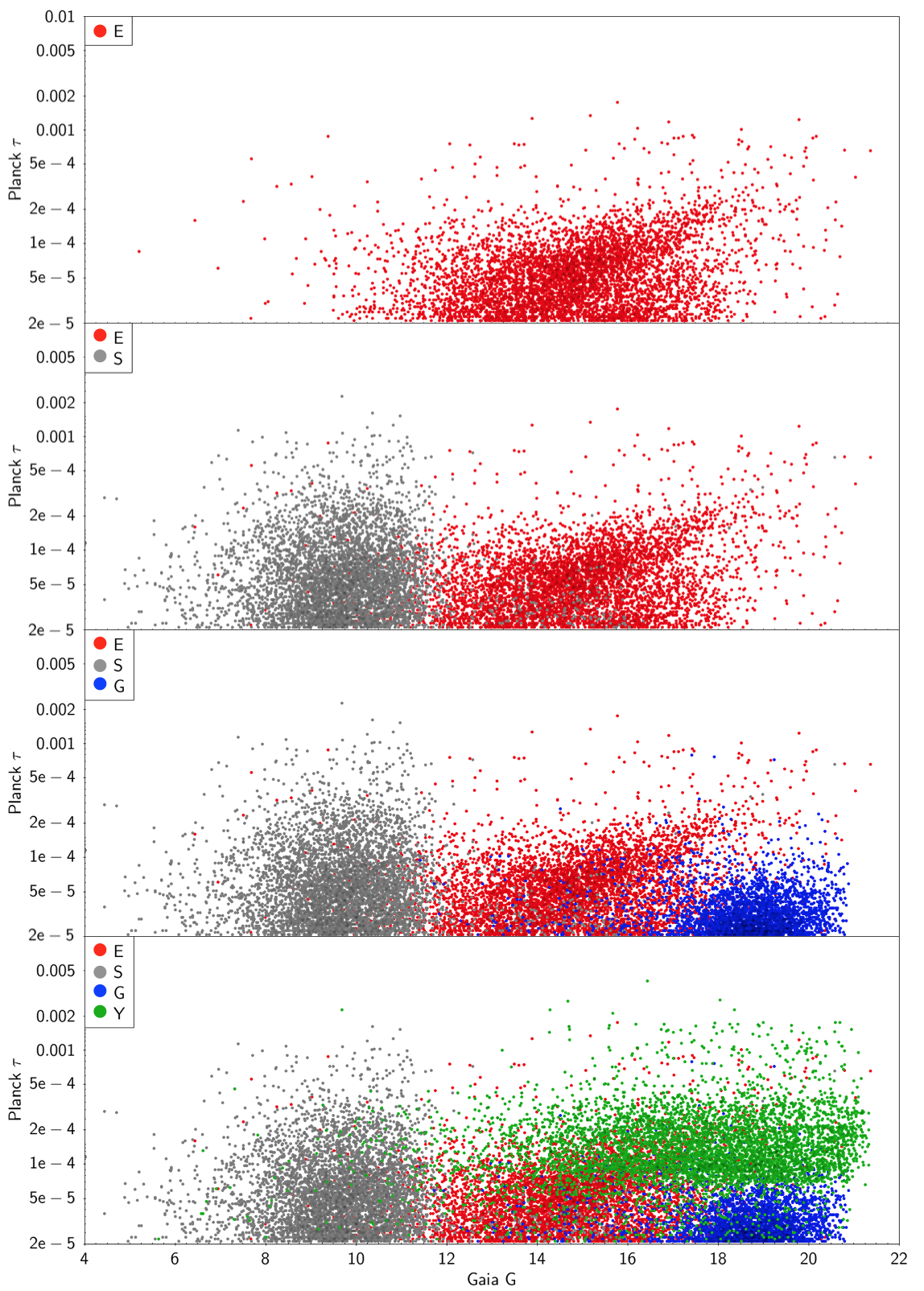
Figure 9: The 4 classes of the objects in the $G$ magnitude–$\tau$ diagram. The top panel shows the distribution of the evolved objects (E) with red dots. They are mostly located at intermediate Gaia $G$ band values, between 12 and 18 magnitudes, and are at lower $\tau$ dust opacity values. On the second panel the main sequence stars (S) are plotted with gray dots. They apper to be brighter than the evolved objects, and a higher fraction is located at high $\tau$ values. On the third panel the extragalactic objects (G) are shown with blue dots and they are at the faint end of the diagram, with low $\tau$ values. On the bottom panel the YSOs (Y) are plotted with green dots. They are mostly faint and at higher $\tau$ values than the extragalactic objects, but lots of them are overlapping with the evolved stars.

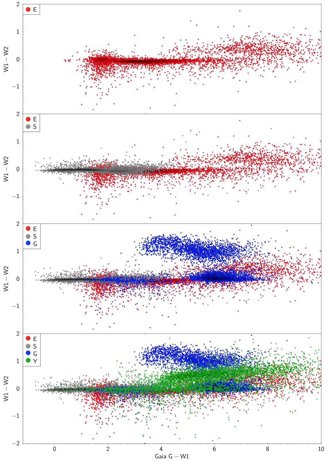
Figure 10: The colors represent the same type of objects as in Figure 9 on the $G-W1$ vs. $W1-W2$ colour-colour plane. Along the $G-W1$ axis the evolved stars are located from 1 to 10. Along the $W1-W2$ axis most of the sources are located around 0, but a smaller cloud of point is visible around 0.5 ranging from 6 to 10 in the $G-W1$ colour. These sources are mostly dominated by Mira type variables, while the others are mostly AGB, RGB and RR Lyr type objects. The main sequence stars have $G-W1$ colours spreading from -0.5 to 4, but their $W1-W2$ colours are very close to 0. In case of the extragalactic sources one can see a bimodial behavior, as well. The objects having $W1-W2$ colours close to 0 are mostly AGN and QSO type sources, while those with $W1-W2$ colours around one are simply indicated in SIMBAD as "Galaxy". The YSOs are mostly redder in both directions, although a bimodial distribution is present for them, too. One cluster of the sources has lower $G-W1$ color index and their $W1-W2$ colour is close to 0, highly overlapping with the main sequence stars. Another cloud of YSO dots is visible at higher $G-W1$ colours and they have a higher $W1-W2$ colour, as well, overlapping with the evolved stars and the extragalactic sources.

The cross-match resulted in 50 001 EG, 182 656 MS, 63 372 E and 14 302 Y class objects that were used to create the training samples. The $G$ band brightness–$\tau$ and the $G-W1$ vs. $W1-W2$ colour-colour diagram of all these sources are plotted in Figure 9 and Figure 10 in Appendix D, representing how the different object types are overlapping in the 2D cuts of the multi-dimensional feature space. For each training sample 14 000 objects of each class were selected randomly. We used equal number of elements from each class to avoid a bias caused by the order of magnitude difference between the different classes. The elements were then permuted and 7 000 objects of each class was selected as the actual training sample, while the remaining 7 000 were used to check the goodness of the classification. The permutation and selection was repeated 10 times, allowing us to have a statistically more meaningful classification procedure.

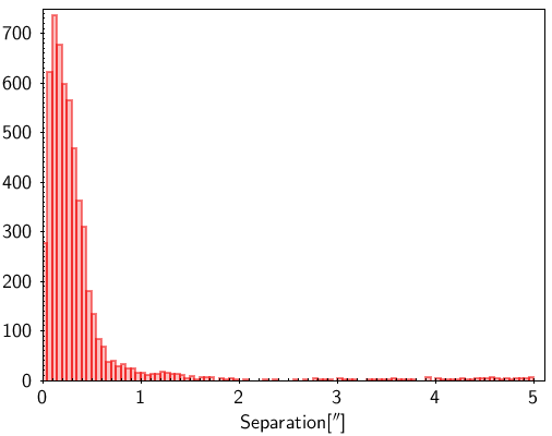
Figure 1: Distribution of angular distance values between the GaiaDR2xAllWISE and the Spitzer YSO catalogue positions. 95% of the matching Spitzer sources are within 1^′′ radius of the DR2 position.

2.4 Classifiers

Classification with supervised methods requires three major steps:

1. Training the classifier

2. Classifying new data with the classifier

3. Tuning the classifier

To do so, several statistical softwares and packages are available for use. In our work we used R (R Core Team 2013), a free software environment for statistical computing and graphics, commonly used in the astronomical community.

We experimented with several classifier methods in order to evaluate their performance and to select the one which is best for our needs. These methods are the Support Vector Machines (SVM, e.g. Solarz et al., 2017; Krakowski et al., 2016; Kurcz et al., 2016; Marton et al., 2016; Heinis et al., 2016; Kovács & Szapudi, 2015; Solarz et al., 2015; Małek et al., 2013; Fadely et al., 2012; Beaumont et al., 2011), the $k$–Nearest Neighbors ($k$–NN, e.g. Pashchenko et al., 2018; Lochner et al., 2016; du Buisson et al., 2015), the Naive Bayes (e.g. Mitchell, 1997; Lochner et al., 2016), Neural Networks (NN Venables & Ripley, 2002) and Random Forests (RF, e.g. Breiman, 2001; du Buisson et al., 2015; Pashchenko et al., 2018).

2.5 Dimension reduction

While all machine learning techniques are capable of handling multi-dimensional datasets, and some of them are capable to assign weights to the features (i.e. the characteristics that define our problem) in order to optimize the classification process and maximize the classification goodness, one should still consider reducing the number of variables. By selecting the relevant features we can shorten the training times, simplify our models, avoid the curse of dimensionality and reduce overfitting of the data. Our initial parameter space contained 39 columns, including the $\tau$ value from the Planck dust opacity map, the Gaia $G$ band brightness value, the 2MASS brightness values, the WISE brightness values, and all the possible colours that can be calculated from the Gaia, 2MASS and WISE photometry.

To reduce the dimensionality of our feature space we calculated the Pearson’s correlation coefficient between each feature and created a correlation plot (see Figure 2 for the YSOs). From the left to right (and top to bottom) the coefficient value was checked and in cases the correlation was above $0.7$ or below $-0.7$, the longer wavelength feature was removed (as typically the angular resolution and background contamination increases with the wavelength). For example, in the Y class training sample (Figure 2) the correlation coefficient value between the Gaia G mag and the 2MASS $J,H$ and $K_{\mathrm{s}}$ magnitudes was 0.88, 0.79 and 0.72, respectively, so all the 2MASS brightness values were removed from the list of features. This procedure was repeated for all the classes. We ended up with the following list of meaningful features for the classes:

• E: $\tau,G,H,W4,G-W4,J-H,K_{\mathrm{s}}-W1,W1-W2,W1-W3$

• EG: $\tau,G,J,W2,W3,G-J,G-W2,J-H,J-K_{\mathrm{s}},H-W2,W2-W3,W3-W4$

• MS: $\tau,G,W4,G-J,G-W4,H-K_{\mathrm{s}},H-W1,H-W3,H-W4,K_{\mathrm{s}}-W2,W1-W2,W1-W3$

• Y: $\tau,G,W1,G-J,G-W4,J-H,H-W1,W1-W2,W1-W3,W2-W4,W3-W4$

Finally, the union of the above features was used in the training sets, resulting in 25 columns instead of the 39 used initially: $\tau,G,J,H,W1,W2,W3,W4,G-J,G-W2,G-W4,J-H,J-K_{\mathrm{s}},H-K_{\mathrm{s}},H-W1,H-W2,H-W3,H-W4,K_{\mathrm{s}}-W1,K_{\mathrm{s}}-W2,W1-W2,W1-W3,W2-W3,W2-W4,W3-W4$.

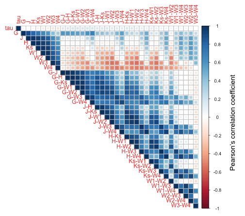
Figure 2: An example of the correlation matrices of the feature space, shown for the Y class (YSOs). Strong correlation is shown with dark blue, strong anti-correlation is shown with dark red colours.

2.6 Metrics

To interpret the results of the different classifiers one has to define metrics that characterizes them in a uniform way. If the predicted class of an object is the same as the true class, i.e. a known YSO is classified as a YSO, we call it a true positive (TP) classification. If the same known YSO is classified as another type of object, then it is a false negative (FN) classification. If an object of an extragalactic nature is classified as a YSO, it is a false positive (FP) classification.

Completeness is the percentage of known YSOs classified as YSO ($N_{\mathrm{TP}}/N$, where N is the number of all objects in the training set), which in ideal case is 100%. In the best case the purity ($N_{\mathrm{TP}}/(N_{\mathrm{TP}}+N_{\mathrm{FP}})$) is also 100%, meaning that all objects from a given object class is classified into their true class, e.g. all known YSOs are classified as YSO, and nothing else is classified as YSO. The contamination is the fraction of false positives among the objects classified as YSO ($N_{\mathrm{FP}}/(N_{\mathrm{TP}}+N_{\mathrm{FP}})$), which is 0% if the classification is perfect.

2.7 Identification of spurious $W3$ and $W4$ AllWISE photometry

The main science goals of the $WISE$ mission were to study infrared-bright galaxies, to find brown dwarfs, and to study near-Earth asteroids. The method of source identification on $WISE$ images is described in the online explanatory supplement and in Marsh & Jarrett (2012). Unfortunately, this method leads to many spurious photometric results in the Galactic plane, which was already investigated in numerous papers (e.g. Koenig & Leisawitz, 2014; Marton et al., 2016; Silverberg et al., 2018). To avoid false classification by the $W3$ and $W4$ band photometry we carried out an analysis similar to what we presented in Marton et al. (2016) based on the findings of Koenig & Leisawitz (2014).

Koenig & Leisawitz (2014) found that the spurious and real detections in the $W3$ and $W4$ bands can be separated by using the following parameters, provided by the AllWISE catalogue:

• Signal–to–noise ratio (SNR) calculated in the $W3$ and $W4$ bands

• The reduced chi-square parameter in the same bands

• The w3m, w4m parameters (the number of individual 8.8s exposures on which a profile-fit measurement of the source was possible)

• The w3nm and w4nm parameters (the number of individual 8.8s exposures on which this source was detected with SNR$>$3)

Koenig & Leisawitz (2014) plotted these parameters and defined a set of criteria to decide if the detection can be accepted as real or if it is rejected and labeled as spurious detection. Instead of defining a set of criteria, we used the Random Forest method to classify the sources into the two classes, but we used the same parameters to separate spurious and real detections in the $W3$ and $W4$ bands.

The training sample for this exercise was created by visually inspecting the $WISE\ W3$ and $W4$ images at the positions of known YSOs. We selected 500 cases where the sources were obviously real and 500 where we could not clearly identify a source. 10 examples for both real and fake sources are presented in Figure 3.

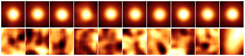
Figure 3: Top row: $WISE\ W4$ images of 10 sources accepted as real ones. Bottom row: $WISE\ W4$ images of 10 sources we labeled as fake sources. All images are centered on the position of known YSOs

3 Results

Below we detail the results of our classification methods. In Section 3.1 we describe how the different methods performed on our training samples including long wavelength WISE data. As explained in Section 2.7 the $W3$ and $W4$ band WISE photometry cannot be trusted in every case, especially in crowded regions with infrared luminous backgrounds where YSOs are typically located. In Section 3.2 we show how well our identification of the spurious WISE photometry worked. In Section 3.3 we describe our classification results obtained without the $W3$ and $W4$ band photometry. Finally, Section 3.4 describe our sample we consider as a reliable YSO candidate catalogue.

3.1 $Gaia$ DR2 x AllWISE source classification including $W3$ and $W4$ WISE photometry

The metrics described in Section 2.6 (completeness, purity, and contamination) were calculated for the YSOs with 13 different methods. SVM was used with 5 different kernels: linear, 2^nd and 3^rd order polynomial, radial and sigmoid. Naive Bayes was used with and without kernel estimation, the $k$-NN method was tried with 3 and 8 nearest neighbours, the Random Forests were used with 500 trees with 5 random variables at each split, 1000 trees with 7 random variables, and 2000 random trees with 10 random variables. Finally, the Neural Networks were also used with its default parameters. We plotted the results of each method in Figure 4 and sorted them according to the purity. The blue bars show the completeness, the green bars show the purity and the red bars stand for the contamination rate.

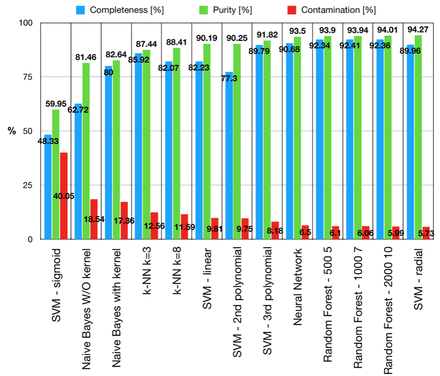
Figure 4: Completeness, purity and contamination rates achieved with different methods to classify the YSO training samples. Methods are in increasing order according to the purity (green bars) achieved with them. Blue bars indicate the completeness, red bars show the contamination rate.

Figure 4 shows that the best classification was achieved by using the Random Forests. In all the three cases (with 500, 1000 and 2000 trees, and 5, 7 and 10 variables tried at each split, respectively) the method performed above 92% completeness for the Y class. The Neural Network also performed above 90%, followed by the 3^rd degree polynomial and the radial basis SVMs, close to 90%.

Not shown in the paper, but we also compared the results achieved with the different methods using the full dataset and after dimension reduction. We found that using a reduced number of features did not improve any classification method significantly, however all of them seem to perform marginally better, except the SVM with sigmoid kernel and the Random Forest with 2000 trees, but the differences between the results is well within the estimated uncertainties.

Our final conclusion was that the best method for our purpose is the Random Forests with 500 trees and 5 random variables tried at each split after dimension reduction.

On Figure 9 and Figure 10 in Appendix D we showed how the four different object types populate the bightness-$\tau$ and colour-colour diagrams. Figure 11 and Figure 12 show the same features for the classified sources. It is apparent that the distribution of the dots is very similar in the two cases.

3.2 Spurious photometry identification in the $W3$ and $W4$ WISE bands

As we described in Section 2.7 the $W3$ and $W4$ detections suffer from fake source identifications and spurious point source photometry. In Section 3.1 we found that the Random Forests with 500 trees and 5 random variables gave us the best results, therefore for the spurious source identification was done with this method, as well.

We found that in all cases the real sources (visually identified on $W3$ and $W4$ images, see Figure 3) were classified as real sources, so the completeness achieved in this exercise was 100%. It also means that none of the real sources was classified as fake source. Among all our tests we found only 2 cases when a fake source was classified as real. This means that the contamination rate was as low as 0.02% and the purity of our real source identification was 99.98%. We note that these results were achieved by accepting that a source is classified as real, if the probability of being real ($P_{R}$) is higher than 0.5.

After applying our classification scheme to the initial dataset (described in Section 2.2) we found that 9 816 124 sources have $P_{R}>0.5$ among the 101 838 724 sources. These are the sources for which we trust the $W3$ and $W4$ photometry listed in the AllWISE catalogue.

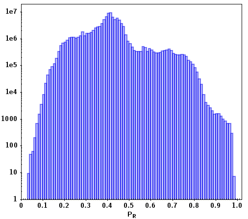
Figure 5: Distribution of probabilities of being a real source ($P_{R}$) among the sources of our initial dataset. 9 816 124 sources were classified as real sources ($P_{R}>0.5$), meaning that their $W3$ and $W4$ photometry can be trusted.

3.3 $Gaia$ DR2 x AllWISE source classification excluding $W3$ and $W4$ WISE photometry

In the previous section (Sect. 3.2) we showed that only 9 816 124 AllWISE sources were classified as real, and the 90.4% of the sources have spurious photometry in the longer wavelength WISE bands. Therefore the classification into the four object classes (EG, MS, Y, E) was repeated, but without any columns containing $W3$ or $W4$ data in the training sets. Again, we used the Random Forest algorithm with 500 trees and 5 random variables at each split. The completeness was 91.78%$\pm$0.28%, the purity was 93.14%$\pm$0.22% and the contamination was 6.86%$\pm$0.22%.

3.4 YSO candidates

Table 1 details the number of sources classified into each object classes depending on the adopted probability threshold of belonging to the given class. Each number is a sum of two numbers:

1. The number of sources belonging to the given object class with $PL$ (classification including longer wavelength $W3$ and $W4$ WISE data) above the threshold and $P_{R}$ (probability of having a real $W3$ and $W4$ photometry greater than 0.5)

2. The number of sources belonging to the given object class with $PS$ (classification excluding longer wavelength $W3$ and $W4$ WISE data) above the threshold and $P_{R}$ (probability of having a real $W3$ and $W4$ photometry lower than or equal to 0.5)

Table 1: Number of sources classified as main sequence star (MS), evolved star (E), extragalactic object (EG) or YSO candidate (Y) with probabilities above the listed thresholds (0.5, 0.9, 0.95, 0.99 and 0.995). Upper table shows the numbers in the case when $W3$ and $W4$ photometry was included and $P_{R}>0.5$. Lower table includes numbers when classification was done without the longer wavelength WISE photometry and $P_{R}\leq 0.5$.

$P_{R}>0.5$	MS	E	EG	Y
$P_{L}\geq$0.50	1 017 841	7 675 537	45 028	528 114
$P_{L}\geq$0.90	458 260	4 252 425	19 235	57 710
$P_{L}\geq$0.95	365 275	2 972 483	16 019	23 502
$P_{L}\geq$0.99	233 647	888 463	8 585	4 946
$P_{L}\geq$0.995	185 416	417 842	5 756	2 885
$P_{R}\leq 0.5$	MS	E	EG	Y
$P_{S}\geq$0.50	1 596 898	47 511 206	14 500 223	12 528 308
$P_{S}\geq$0.90	62 710	8 224 488	59 375	1 710 918
$P_{S}\geq$0.95	35 245	3 544 466	40 068	235 995
$P_{S}\geq$0.99	14 277	430 306	19 706	15 942
$P_{S}\geq$0.995	8 219	169 504	12 683	7 408

We found 1 768 628 sources that were classified as potential YSO candidates, meaning that $P_{R}>0.5$ and $PL_{Y}\geq 0.9$ or $P_{R}\leq 0.5$ and $PS_{Y}\geq 0.9$. Our results are published in a form of a VizieR table. The table contains the Gaia source IDs, the AllWISE source designations, the Gaia, 2MASS and WISE photometric data. For each source the membership probabilities are also listed in the table. These probability values are the $P_{R}$ values (probability of having a real $W3$ and $W4$ photometry), the classification probabilities using all $WISE$ bands ($PL_{MS}$, $PL_{E}$, $PL_{EG}$, $PL_{Y}$) and the classification probabilities including only the shorter wavelength $WISE$ bands ($PS_{MS}$, $PS_{E}$, $PS_{EG}$, $PS_{Y}$). Because all these data are provided, users can decide about the thresholds for themselves according to the needs of their scientific study.

4 Discussion

4.1 Application of the YSO selection to Orion A

Recently Großschedl et al. (2018) analysed the 3D structure of the archetypal molecular cloud, Orion A based on Gaia DR2 data. Their results show that Orion A is not a straight filamentary cloud as it appears in the sky, but has a cometary-like shape. It has two components, a denser head at $\sim$400 pc, and a longer tail with fewer young stars reaching out to $\sim$470 pc. We repeated their analysis but instead of using the YSOs defined in their study, we used our own YSO candidates. We started with sources we classified as YSOs candidates and created a pre-selection of the sample by applying the parallax criteria of Großschedl et al. (2018) to these sources. Moreover, we restricted our analysis to sources located between 300 and 600 pc according to the distance estimate of Bailer-Jones et al. (2018). As a result we ended up with 1 368 objects, plotted on the Herschel/PACS images of Orion A in Figure 6.

Figure 7 shows the median distance value of the YSO candidates calculated in $0^{\circ}.5$ bins along the galactic longitude. Our results (green line) show a very good agreement with those of Großschedl et al. (2018) presented with the black line and confirm that the head part of the cloud is located at a distance of $\sim$380–400 pc while the tail part is reaching out to $\sim$430–480 pc. We obtained similar results when using all our YSO candidates between 300 and 600 pc distance without the parallax criteria (red line). As a comparison we overplotted those sources classified as main-sequence stars (blue line) and found that their distribution is different than that of the YSOs.

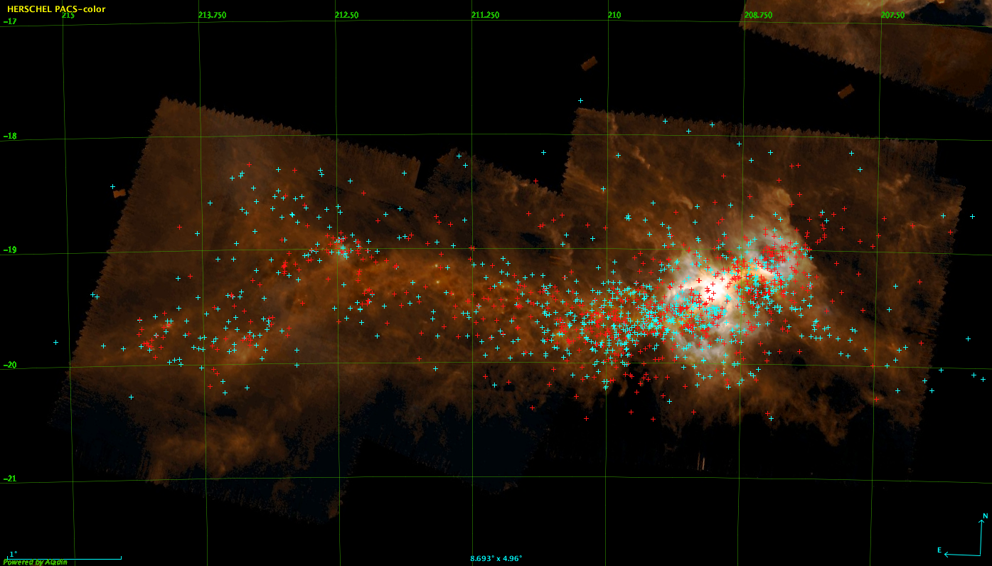
Figure 6: Our YSO candidates (cyan crosses) in Orion A overlaid on a false-color Herschel/PACS image, using galactic frame. 1 368 YSO candidates are selected after applying the parallax criteria of Großschedl et al. (2018) and restricting their distance between 300 and 600 pc. 682 YSOs of Großschedl et al. (2018) are overplotted with red crosses.

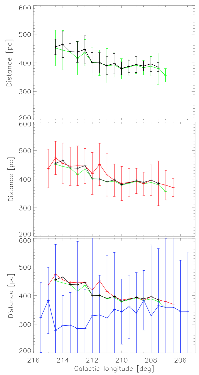
Figure 7: Median distance of the YSO candidates in Orion A as a function of the galactic longitude. The median of the distances were calculated in $0^{\circ}.5$ bins. The error bars represent the standard deviation of the distance values in the bins. The sample of Großschedl et al. (2018) is plotted with black. Our YSO sample with the parallax criteria of Großschedl et al. (2018) applied is shown with green. The red line present the median distance value of all of our 2 668 YSO candidates in the region (without parallax criteria, but located between 300 and 600 pc). The blue line presents the distance distribution of the 669 sources classified as main-sequence stars (MS). They are distributed in a more homogeneous way as a function of distance, therefore the error bars are larger than for the YSOs.

This field was also used to validate the purity of our selection in two ways. First, we looked for counterparts of the Großschedl et al. (2018) catalogue of 682 YSOs in our initial sample, using a 1^′′ search radius. 568 matches were found. 517 of them (90%) were classified as YSO candidate by our method. 263 of them were classified as real ($P_{R}>0.5$) with $PL_{Y}\geq 0.9$, and 254 not real ($P_{R}\leq 0.5$) with $PS_{Y}\geq 0.9$. Figure 8 shows the 682 Großschedl et al. (2018) sources and our YSO candidates. The distribution of the two datasets are very similar.

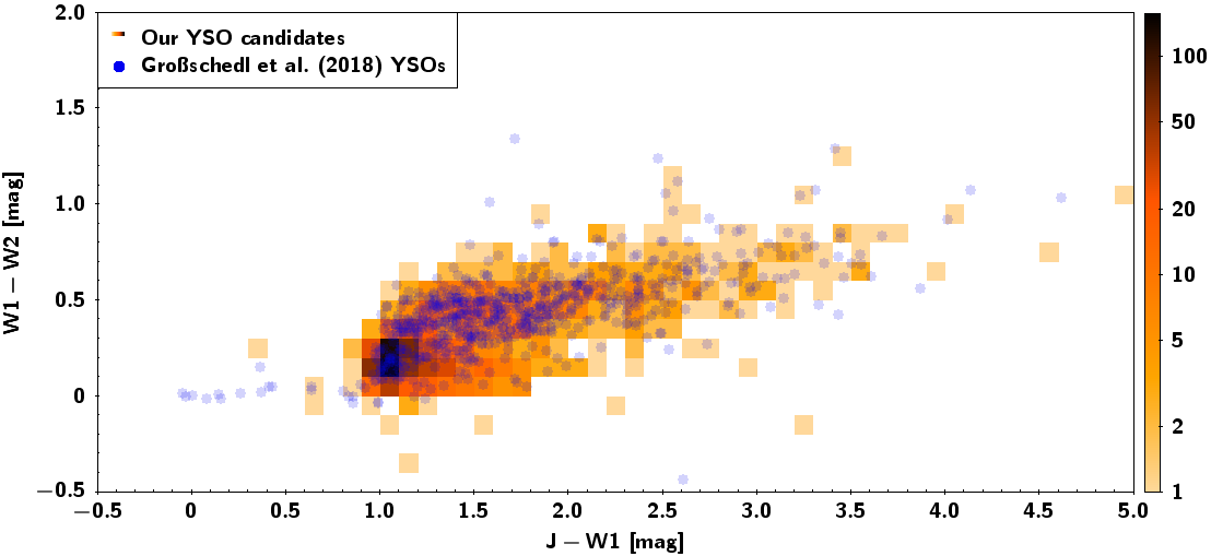
Figure 8: YSOs from the Großschedl et al. (2018) catalogue (blue opaque dots) and the surface density of our sources classified as YSO candidates (red colour coding) on the 2MASS $J$-$WISE$ $W1$ vs. $WISE$ $W1-W2$ colour-colour diagram. The surface density was calculated in bin size of 0.1 in both directions.

As an additional sanity test of our YSO classification, we cross-matched the 2 668 YSO candidates in this region (these are YSO candidates located between 300 and 600 pc distance selected without applying any criterion based on parallax) with the SIMBAD database, and found 1 701 pairs using 5^′′ search radius. We found that 1 212 (71.3%) sources are either YSOs, YSO candidates, T Tau stars, pre-main sequence stars, or Orion-type variables. Additional 412 sources (24.2%) are stars in clusters, stars in nebulae, emission line stars, flaring stars, infrared sources and objects indicated as variable or irregular variable stars. These can also be interpreted as objects having properties similar to those of potential YSOs. 53 objects (3.1%) are listed simply as “star” and 24 (1.4%) were found to be classified by SIMBAD as some other type of object. Only one of the sources is known to be a BY Dra type object which is a late-type star, and no extragalactic object was found.

4.2 YSO candidates among the Gaia Photometric Science Alerts

As Gaia is monitoring the whole sky and collecting data, it detects transients and sudden brightness changes and is able to provide alerts to the astronomical community in almost real-time (Wyrzykowski et al., 2012). The alerting system runs on a daily basis at the Institute of Astronomy in Cambridge (part of the Gaia Data Processing and Analysis Consortium, DPAC). The Nominal Scanning Law defines the observing strategy across the sky. It is a pattern optimised for the final astrometric solution (Lindegren et al., 2012), and ensures that most of the stars will obtain, on average, about 70 measurements at different scanning angles. However, some areas of high stellar density such as the Galactic Bulge will only have about 50 measurements during the entire mission (Wyrzykowski et al., 2012).

The $\sim$70 brightness values are enough to be sure that Gaia detects numerous very rare events like outbursts of FUor or EXor-type young stars, of which only a handful is known (Aduard et al., 2014). Identification of potential YSO candidates can help the decision tree of the pipeline to promote a target with possible outbursts and fadings due to the circumstellar disk. Whenever an alert is made for such an object, the data can be made available, allowing for continuous follow-up of the candidate YSO. As of 2019 April 8^th the Gaia Photometric Science Alerts database includes 7 670 objects. 131 of them are known to be of YSO nature.

We used a 1^′′ radius to match the alerts database to our Initial Dataset (Section 2.2). As a result we found 187 matching sources. The reason for finding only 187 objects is described below:

1. The alerts are dominated by new sources, that were previously unseen and DR2 contains data collected from the first 22 months of the mission. As a result, only 1 959 out of all the alerts have a DR2 counterpart.

2. Only 1 012 of them had AllWISE counterparts.

3. As explained in Section 2.2 we classified only those sources that are located in dusty environments and the Planck dust opacity value is above 1.3$\times 10^{-5}$ and they fulfill our quality criteria (i.e. have photometric data in all bands and only one Gaia source belongs to a given AllWISE ID), as well. Only 251 sources have met our requirements.

84 of the 251 matching sources were classified as YSO candidates with $P_{R}>0.5$ and $PL_{Y}\geq 0.9$, or $P_{R}\leq 0.5$ and $PS_{Y}\geq 0.9$. In Table LABEL:tab:classifiedysoalerts we listed their main properties. In case the nature of the alerted object is known, it is listed on the Alerts Index webpage. From the 84 object we classified as YSO candidates 44 were already known to be confirmed YSOs or YSO candidates. The other 40 sources had unknown object classes. This means that none of the alerts we classified as YSO candidates were known to be any different kind of object, e.g. Mira, cataclysmic variable, supernova, etc.

Table 2: Gaia Science Alerts classified as YSO candidates with $PL_{Y}\geq 0.9$ and $P_{R}>0.5$ or with $PS_{Y}\geq 0.9$ and $P_{R}\leq 0.5$ according to our method. The columns are as follows: 1. Alert name as issued by the Alerts Index webpage, 2. Date and time of the alerting observation, 3.-4. RA and Dec, 5. object class based on literature, 6. probability of being a YSO according to our classification when WISE W3 and W4 photometry is included, 7. probability of being a YSO according to our classification when WISE W3 and W4 photometry is not used in the classification, 8. the probability of the WISE WISE W3 and W4 photometry being real, 9. Gaia DR2 source ID

Name	Date	RA	Dec	Class	$PL_{Y}$	$PS_{Y}$	$P_{R}$	$Gaia$ DR2 ID
Gaia19bez	2019-04-01 23:49:11	83.70199	-5.70783	YSO	0.9998	0.9994	0.47	3017244319631273856
Gaia19bdw	2019-03-29 22:34:24	161.67619	-60.16919	YSO	0.9552	0.94	0.492	5350284122620723072
Gaia19azy	2019-03-15 21:39:49	244.35307	-36.95937	YSO	0.991	0.8764	0.65	6021662385163163648
Gaia19axm	2019-03-07 03:27:42	275.5886	-15.80299	unknown	0.9918	0.9874	0.35	4097852452014666368
Gaia19axl	2019-02-08 12:15:35	83.85629	-5.76245	YSO	0.9984	0.996	0.632	3017245144265120384
Gaia19axj	2019-02-15 12:39:42	87.26549	22.45243	unknown	0.9052	0.82	0.592	3427267972452130432
Gaia19awc	2019-03-05 03:14:14	273.90055	-2.25697	unknown	0.8174	0.9072	0.19	4270884761539465344
Gaia19avm	2019-03-04 06:05:39	89.31937	-9.71695	unknown	0.791	0.9264	0.224	3011393165424898176
Gaia19avc	2019-03-04 20:16:36	100.20506	9.74441	YSO	0.9828	0.9872	0.612	3326712411412675968
Gaia19avb	2019-02-08 18:08:24	90.94027	-9.6506	YSO	0.9638	0.9256	0.55	3005362103626941312
Gaia19ars	2019-02-17 13:34:44	24.26503	65.00039	unknown	0.997	0.9978	0.51	513080267819937920
Gaia19arj	2019-02-19 13:34:26	38.12432	72.60243	YSO	0.9892	0.9824	0.538	545882891555329536
Gaia19aqr	2019-02-18 08:26:58	302.77041	33.91837	unknown	0.9068	0.9242	0.594	2055635703663536640
Gaia19aqi	2019-01-17 19:00:23	162.34187	-59.18257	YSO	0.8814	0.928	0.428	5350433523059602304
Gaia19apz	2019-02-16 21:26:00	274.24053	-19.89191	unknown	0.9776	0.996	0.356	4094447401937531648
Gaia19apd	2019-02-14 09:59:19	242.09364	-39.0797	YSO	0.9994	0.9994	0.704	5997082867132347136
Gaia19apa	2019-02-12 18:32:03	83.21928	12.91914	unknown	0.9546	0.9382	0.47	3341084265336119552
Gaia19ant	2019-02-10 06:10:16	93.21496	-6.18144	YSO	0.986	0.995	0.56	3019875657114864384
Gaia19anj	2019-02-09 00:16:26	84.51622	-4.27858	YSO	0.9964	0.9728	0.516	3215624048669350016
Gaia19anf	2019-02-08 06:14:49	84.12543	-6.38611	YSO	0.9998	0.9996	0.546	3016949616153731584
Gaia19amy	2019-02-08 06:14:38	84.03455	-6.81008	YSO	0.9974	0.9978	0.562	3016920066778758528
Gaia19ajk	2019-01-29 22:04:15	300.39781	35.72513	YSO	0.9174	0.9012	0.398	2059471349978080256
Gaia19aik	2019-01-27 04:01:31	303.68998	40.25742	unknown	0.906	0.9194	0.688	2062414368951680000
Gaia19ace	2019-01-05 20:20:26	59.0241	53.6004	YSO	0.8828	0.9812	0.386	252155434006298112
Gaia18eay	2018-12-29 02:16:38	43.59314	58.61324	unknown	0.9504	0.9496	0.518	461362844316408704
Gaia18ead	2018-12-27 08:25:57	22.44645	68.47463	unknown	0.9342	0.9242	0.592	532063610946188416
Gaia18dvz	2018-12-18 01:28:32	129.72988	-40.68815	YSO	0.9768	0.9734	0.568	5528238468964304512
Gaia18dvs	2018-12-14 08:38:32	302.93063	27.82686	unknown	0.9844	0.9762	0.514	1836621822164584832
Gaia18drz	2018-12-04 08:37:50	285.61527	9.02441	YSO	0.9966	0.997	0.538	4310567510575660928
Gaia18dlu	2018-11-17 09:06:29	304.4854	41.71411	unknown	0.9864	0.9868	0.458	2068593448191217920
Gaia18dli	2018-11-16 06:12:45	135.80023	-47.82651	unknown	0.9828	0.968	0.464	5327027733703518720
Gaia18dhk	2018-11-04 18:36:05	199.71135	-63.98177	unknown	0.938	0.9668	0.542	5859151160662602752
Gaia18dhf	2018-11-05 00:35:50	200.24079	-63.24464	unknown	0.9674	0.97	0.492	5868194094041412096
Gaia18dgx	2018-11-03 12:31:44	189.92875	-62.96378	YSO	0.9702	0.9708	0.552	6055161579577825280
Gaia18dag	2018-10-13 02:57:42	284.53971	3.01279	unknown	0.9856	0.996	0.428	4280720889482000128
Gaia18czn	2018-10-10 18:17:19	84.30843	-7.06144	YSO	1.0	0.9994	0.534	3016853443246145792
Gaia18czm	2018-10-10 13:43:35	98.08678	5.07122	YSO	0.9938	0.989	0.332	3131338717100881024
Gaia18cvo	2018-09-30 08:25:28	256.4861	-46.40277	unknown	0.9786	0.9772	0.62	5962994536340143360
Gaia18cvc	2018-09-28 17:29:57	67.07812	48.57304	unknown	0.9908	0.9938	0.362	258093106034362368
Gaia18cqd	2018-09-13 00:00:51	49.9249	11.50455	unknown	0.7004	0.903	0.456	17030889653951616
Gaia18cpz	2018-09-12 07:20:32	129.11882	-39.2163	unknown	0.9992	0.9986	0.466	5528691566536872320
Gaia18cpd	2018-09-09 22:17:33	301.45445	28.84617	unknown	0.9518	0.9388	0.66	2029135824162001536
Gaia18cpb	2018-09-09 22:13:57	298.16966	27.10213	unknown	0.9456	0.9604	0.464	2027177392100413440
Gaia18cnc	2018-09-02 23:36:02	62.38696	48.02058	unknown	0.9844	0.9698	0.234	246335718959842688
Gaia18cls	2018-08-30 07:23:50	135.70595	-46.74502	unknown	0.8928	0.9226	0.426	5330182610521277440
Gaia18cgq	2018-08-16 03:09:08	271.04164	-24.32494	YSO	0.9854	0.9838	0.136	4065976338621931136
Gaia18ccp	2018-08-10 08:59:12	257.91176	-36.03637	unknown	0.9526	0.9438	0.636	5977001696005980672
Gaia18cbh	2018-08-06 09:05:10	236.374	-34.39422	YSO	0.9524	0.8986	0.554	6014692477866901760
Gaia18cac	2018-08-03 08:46:10	239.26591	-54.15523	YSO	0.986	0.9708	0.462	5884723980058860544
Gaia18byl	2018-07-30 17:40:01	37.72747	59.5787	unknown	0.9414	0.922	0.546	465085344014342400
Gaia18bxx	2018-07-28 11:26:18	37.33175	73.03989	YSO	0.9758	0.9858	0.576	546658352195182464
Gaia18bwj	2018-07-23 23:39:00	343.37586	62.63983	YSO	0.964	0.9222	0.562	2207276292913481856
Gaia18bvw	2018-07-22 02:38:35	149.54376	-58.17488	unknown	0.9706	0.986	0.544	5259160275404381440
Gaia18bre	2018-06-26 23:47:00	313.22393	44.24919	YSO	0.9354	0.9422	0.568	2162939208074527616
Gaia18bjd	2018-05-27 19:36:51	15.81917	61.61695	YSO	0.998	0.9954	0.57	522714223060690432
Gaia18bgs	2018-05-17 09:53:56	106.14958	-11.08006	YSO	0.9916	0.9626	0.546	3046430340396482176
Gaia18bfz	2018-05-14 22:05:55	98.53708	4.49401	unknown	0.9978	0.999	0.458	3130544384371982336
Gaia18beu	2018-05-09 09:55:25	88.6581	1.49764	YSO	0.9996	0.9984	0.652	3315789764117572224
Gaia18bdn	2018-05-04 15:42:22	83.49683	-5.7731	YSO	0.9208	0.9362	0.598	3017253871638555520
Gaia18avw	2018-04-03 23:56:14	39.71863	66.43154	unknown	0.9524	0.9418	0.512	516596707858306944
Gaia18asj	2018-03-23 22:55:50	79.91252	7.75051	YSO	0.9336	0.885	0.626	3241408897713545472
Gaia18arc	2018-03-19 15:44:50	134.72185	-49.22867	YSO	0.9418	0.9764	0.376	5325391385523762048
Gaia18afm	2018-01-19 14:55:30	298.60582	28.07414	unknown	0.9334	0.9972	0.432	2028360878957519744
Gaia17ccn	2017-08-20 11:32:05	101.18753	0.22775	unknown	0.9296	0.9148	0.442	3125506215936019072
Gaia17byj	2017-08-02 04:40:04	82.3732	37.09014	unknown	0.9922	0.9858	0.534	184279626286154496
Gaia17bxn	2017-07-29 13:47:25	254.53228	-40.96615	unknown	0.9522	0.9686	0.63	5966671582407739008
Gaia17bse	2017-07-04 16:44:46	305.20584	39.65007	YSO	0.9346	0.9704	0.28	2061491255911833088
Gaia17bns	2017-06-13 15:30:16	131.04029	-41.33341	YSO	0.9946	0.997	0.394	5525226180763038336
Gaia17bnf	2017-06-11 16:49:37	320.56135	49.09411	unknown	0.9994	0.9988	0.55	2165017456849422080
Gaia17aqb	2017-03-07 19:16:04	314.37986	44.04373	YSO	0.9636	0.9654	0.548	2162145223244439168
Gaia17afn	2017-01-21 08:39:05	83.78629	-4.7812	YSO	0.9706	0.9622	0.542	3209576459840251776
Gaia17afi	2017-01-20 08:37:02	83.94619	-6.19588	YSO	0.9986	0.998	0.198	3017166907140903040
Gaia17afh	2017-01-20 08:35:56	84.72033	-7.00669	YSO	0.9876	0.9948	0.57	3016107798267446528
Gaia16bqh	2016-10-26 19:07:28	68.21489	54.22959	unknown	0.9602	0.9554	0.512	273955008670915328
Gaia16bpa	2016-10-18 04:31:25	272.45945	-21.76201	unknown	0.9912	0.9992	0.468	4069775842794238976
Gaia16bmg	2016-10-07 18:17:57	346.65814	61.00646	unknown	0.969	0.9876	0.56	2014871722373659776
Gaia16blg	2016-10-03 06:02:50	315.26076	52.45242	YSO	0.999	0.9994	0.598	2170293158455917440
Gaia16bft	2016-09-06 20:10:30	53.13751	31.03934	YSO	1.0	0.9992	0.536	121163093300288256
Gaia16apz	2016-05-22 14:20:39	343.5964	61.84157	YSO	0.8808	0.994	0.49	2206993787141103488
Gaia16ama	2016-04-26 04:01:06	344.98905	62.4256	unknown	0.9144	0.9988	0.498	2207037973764265472
Gaia16aly	2016-04-27 06:43:37	100.14171	9.80808	YSO	0.9746	0.986	0.148	3326716534581491840
Gaia16alt	2016-04-23 10:05:23	325.74996	66.19105	YSO	0.9966	0.9948	0.596	2218013543651547904
Gaia16ajp	2016-03-29 06:40:07	105.65842	-11.49547	unknown	0.9942	0.988	0.182	3046035130386309888
Gaia16agv	2016-02-29 13:04:14	83.69805	-5.96583	YSO	0.9946	0.9894	0.608	3017188931733323776
Gaia16agu	2016-02-29 13:02:36	85.10685	-7.09369	YSO	0.9746	0.9604	0.64	3016110860580352128

We also studied those 129 alerts that were already known to be YSOs, and checked how our classification performed in those cases. Previously we accepted a source as a YSO candidate if $P_{R}>0.5$ and $PL_{Y}\geq 0.9$, or $P_{R}\leq 0.5$ and $PS_{Y}\geq 0.9$. Among these objects we found 15 that were not accepted as YSO candidates. We listed them in Table 3. Among these 15 cases we found only four cases where $PL_{Y}<0.5$ and also $PS_{Y}<0.5$:

• Gaia18ale ($PL_{Y}$=0.25, $PS_{Y}$=0.15) is also a red Galactic plane source that was classified as YSO in Marton et al. (2016)

• Gaia16aez ($PL_{Y}$=0.24, $PS_{Y}$=0.24) is a source known to the SIMBAD database as a YSO and was first listed as a young star by Herbig & Dahm (2002)

• Gaia19agd ($PL_{Y}$=0.14, $PS_{Y}$=0.09) is identified in the ASAS-SN system as an AGN or YSO, but is listed in multiple extragalactic catalogues in the VizieR database (e.g. Liai et al., 2019).

• Gaia18adm ($PL_{Y}$=0.06, $PS_{Y}$=0.09) is listed on the Alerts Index webpage as a possible YSO, but is classified as a possible AGN by Edelson & Malkan (2012).

Table 3: All Gaia Science Alerts already known to be YSOs and found among our DR2 sources. Only 12 of them was classified as YSO candidate with $P_{Y}<0.9$ by our method, and only 4 of those have $P_{Y}<0.5$. The columns are as follows: 1) Alert name as issued by the Alerts Index webpage, 2) Date and time of the alerting observation, 3)-4) RA and Dec, 5)-6) probability of being a YSO according to our classification and its error, 7) Gaia DR2 source ID

Name	Date	RA	Dec	$PL_{Y}$	$PS_{Y}$	$P_{R}$	$Gaia$ DR2 ID	Comment
Gaia19ave	2019-02-17 00:25:12	100.03513	9.99052	0.6802	0.6804	0.43	3326910568319185408	known YSO 2MASS J06400842+0959259 fades by 1.6 mag
Gaia19ape	2019-02-14 10:54:41	277.46865	-3.94831	0.665	0.6706	0.528	4257893967232850304	candidate YSO dims by 0.6 mag
Gaia19ajj	2019-01-29 05:25:01	122.69077	-36.07526	0.8866	0.8312	0.49	5544564391276237312	Gaia star (possible YSO) brightens by 5 mags over 3 years
Gaia19agd	2019-01-19 02:22:19	327.40184	65.62713	0.1374	0.093	0.548	2219241148384022528	YSO brightens by 1.5 mag
Gaia18dnb	2018-11-20 11:40:51	106.15048	-11.26449	0.7266	0.7582	0.536	3046408758180843264	candidate YSO brightens by 0.7 mag in ~1 month
Gaia18bpt	2018-06-20 16:52:58	182.60228	-61.75732	0.8776	0.9068	0.61	6057768865245322240	Gaia source coincident with candidate YSO shows gradual decline of almost 2 mags
Gaia18bfo	2018-05-14 10:14:45	98.66708	14.03232	0.559	0.4688	0.43	3355671456041735808	YSO brightens by 2 mags
Gaia18asa	2018-03-21 06:29:28	328.05148	47.2505	0.7936	0.7824	0.28	1974730133391256832	1 mag fading of red Gaia source, previous dips in light curve. Possible YSO
Gaia18apr	2018-03-12 06:00:09	11.05205	55.15218	0.5646	0.582	0.594	418322186771625344	erratic variable Gaia source brightens by 2.5 mags over 500 days, candidate YSO/AGN
Gaia18ale	2018-02-11 14:24:14	278.02124	-20.84946	0.2486	0.1482	0.686	4091843208674333824	1.8 mag increase in variable red candidate YSO
Gaia18ajf	2018-02-05 08:27:11	261.90538	-24.12577	0.3876	0.51	0.494	4111263818162632960	variable red Galactic plane source brightens by >1 mag, candidate YSO (Marton et al.)
Gaia18aiq	2018-02-05 00:28:58	109.55913	-23.72759	0.5744	0.3822	0.39	5617801486411760000	2 mag rise on previously variable Galactic Plane source, strong WISE signal, probably YSO
Gaia18adm	2018-01-13 10:10:38	126.44875	-34.15915	0.0568	0.087	0.608	5543700827969368320	possible YSO (showing dips), declines by 1 magnitude
Gaia17bvo	2017-07-23 07:38:32	238.2645	-52.40214	0.8212	0.5944	0.248	5981188808079578624	0.5 mag brightening of Galactic plane variable source, candidate YSO
Gaia16aez	2016-02-19 16:32:26	328.37432	47.30115	0.242	0.2394	0.396	1974546686752048768	sudden drop in flux in YSO 2MASS J21532984+4718041

We also checked the database of the unpublished Gaia alerts for sources we classified as YSO candidates. The database includes 6 802 636 sources as of 2019 April 9^th. Using a 1^′′ matching radius 6 450 matching sources were found. This large number suggests that likely many more YSOs show brightness variations and shows the potential of the analysis of Gaia light curves once they become public.

5 Summary

In this paper we presented a classification of those sources in the Gaia DR2 catalogue that have a counterpart in the AllWISE catalogue. Robust samples of known main–sequence stars, evolved stars, extragalactic objects and YSOs were built to create clean dataset including Gaia, 2MASS and WISE photometry. We used these datasets as training samples for several machine learning algorithms and tested them to find the method best working for our purposes.

We found that Random Forests with 500 trees and 5 random variables tried at each split gives the best results. For all 101 838 724 sources of our initial sample the classification was done, first by including longer-wavelength $W3$ and $W4$ WISE photometric data, then by excluding them. Latter classification was necessary, because the $W3$ and $W4$ photometric data are unreliable in many cases in crowded regions, where YSOs are typically found. In order to decide if the $W3$ and $W4$ photometric data is reliable, we visually inspected $W3$ and $W4$ images of YSOs, created a Random Forest classifier and for all sources we calculated the probability of having reliable detections in those bands.

All our results, including the classification probabilities, source IDs and photometric data are publicly available through the VizieR service.

Our careful validation process showed that we are able to recover $\sim$92% of the known YSOs and the fraction of sources false positively classified as YSO candidates is around 6%. Our method was successfully tested in a realistic scenario, the Orion A star forming region. The results are in excellent agreement with that of Großschedl et al. (2018), confirming the 3D structure of Orion A.

We also used our classification to identify previously unknown YSO candidates in the Gaia Photometric Science Alerts System and were able to add 40 more to the list of 130 YSO alerts, significantly increasing their number. A more detailed analysis of YSO light curves based on this classification and YSO identification will be helpful to improve our understanding of YSO variability, disk evolution and planet formation theories and models. Also, the alerting algorithms can benefit: the AlertPipe of Gaia and future telescopes can be more sensitive to YSO events triggering more alerts for the detailed follow-up observations.

Appendix A Photometric YSO catalogues found in the VizieR database

Allen et al. (2012), Billot et al. (2010), Connelley et al. (2008), Evans et al. (2009), Furlan et al. (2016), Gutermuth et al. (2008), Gutermuth et al. (2009), Jose et al. (2017), Kirk et al. (2009), Kun et al. (2016b), Lada et al. (2017), Rebull et al. (2011), Saral et al. (2017)

Appendix B Spectroscopic YSO catalogues listed by VizieR

Alcala et al. (2014), Ansdell et al. (2016, 2017), Connelley & Greene (2010), Cooper et al. (2013), Dzib et al. (2015), Erickson et al. (2015), Fang et al. (2009), Frasca et al. (2017), Kim et al. (2016), Kumar et al. (2014), Kun et al. (2009), Kun et al. (2016a), Oliveira et al. (2009), Pascucci et al. (2016), Rebollido et al. (2015), Szegedi–Elek et al. (2013)

Appendix C YSO related Spitzer publications

Alcalá et al. (2008), Allen et al. (2008), An et al. (2011), Balog et al. (2007), Broekhoven-Fiene et al. (2014), Bryden et al. (2009), Chavarria et al. (2008), Chen et al. (2011), Chen et al. (2012), Cieza et al. (2007), Cloutier et al. (2014), Cody et al. (2014), Dahm & Hillenbrand (2007), Dewangan & Anandarao (2011), Dunham et al. (2015), Flaherty et al. (2013), Harvey et al. (2007), Hernández et al. (2007a), Hernández et al. (2007b), Hernández et al. (2008), Jose et al. (2016), Koenig et al. (2008), Kounkel et al. (2016), Lada et al. (2006), López-García et al. (2013), Luhman et al. (2008), Luhman et al. (2010), Megeath et al. (2012), Merín et al. (2008), Muench et al. (2007), Oliveira et al. (2010), Oliveira et al. (2013), Peterson et al. (2011), Puga et al. (2009), Ragan et al. (2009), Rapson et al. (2014), Rebull et al. (2010), Rivera–Ingraham et al. (2011), Roccatagliata et al. (2011), Samal et al. (2012), Saral et al. (2015), Stelzer & Scholz (2009), Strafella et al. (2010), van der Marel et al. (2016), Willis et al. (2013), Winston et al. (2007), Young et al. (2015)

Appendix D Brightness – $\tau$ and colour – colour diagrams

Figure 11: Position of the unknown sources in the same $G$ brightness–$\tau$ diagram as in Figure 9 after we classified them into the 4 object classes. Only those objects are plotted which were classified into the corresponding classis with $P\geq 0.9$. The position of the sources is very similar to those in Figure 9.

Figure 12: Position of the unknown sources in the same $G-W1$ vs. $W1-W2$ colour–colour diagrams as in Figure 10 after we classified them into the 4 object classes. As in Figure 11, only those objects are plotted which were classified into the corresponding classis with $P\geq 0.9$. The position of the sources is very similar to those in Figure 10, and the same substructures can be identified on the diagrams.

References

- Ábrahám et al. (2009) Ábrahám, P., Juhász, A., Dullemond, C. P. et al. 2009, Nature, 459, 224
- Aduard et al. (2014) Audard, M., Ábrahám, P., Dunham, M. M. et al. 2014, Protostars and Planets VI, University of Arizona Press, Tucson, 914 pp., p.387-410
- Alcalá et al. (2008) Alcalá, J. M., Spezzi, L., Chapman, N. et al. 2008, ApJ, 676, 427
- Alcala et al. (2014) Alcalá, J.M., Natta A.; Manara C.F. et al. 2014, A&A, 561, 2
- Allen et al. (2008) Allen, T. S., Pipher, J. L., Gutermuth, R. A. et al. 2008, ApJ, 675, 491
- Allen et al. (2012) Allen, T. S., Gutermuth, R. A., Kryukova, E. et al. 2012, ApJ, 750, 125
- An et al. (2011) An, D., Ramírez, S. V., Sellgren, K. et al, 2011, ApJ, 736, 133
- Ansdell et al. (2016) Ansdell, M., Williams, J. P., van der Marel, N. et al. 2016, ApJ, 828, 46
- Ansdell et al. (2017) Ansdell, M., Williams, J. P., Manara, C. F. et al. 2017, AJ, 153, 240
- Armitage et al. (2001) Armitage, P. J., Livio, M., & Pringle, J. E. 2001, MNRAS, 324, 705
- Armitage et al. (2019) Armitage, T. J., Kay, S. T. & Barnes, D. J. 2019, MNRAS, 484, 1526
- Bailer-Jones et al. (2018) Bailer-Jones, C. A. L., Rybizki, J., Fouesneau, M., Mantelet, G. & Andrae, R. 2018, AJ, 156, 58
- Balog et al. (2007) Balog Z., Muzerolle J., Rieke G. H. et al. 2007, ApJ, 660, 1532
- Baraffe, Chabrier, & Gallardo (2009) Baraffe, I., Chabrier, G. & Gallardo, J. 2009, ApJ, 702, L27
- Beaumont et al. (2011) Beaumont, C. N., Williams, J. P., & Goodman, A. A. 2011, ApJ, 741, 14
- Bell & Lin (1994) Bell, K. R., & Lin, D. N. C. 1994, ApJ, 427, 987
- Billot et al. (2010) Billot, N., Noriega-Crespo, A., Carey, S. et al. 2010, ApJ, 712, 797
- Bonnell & Bastien (1992) Bonnell, I., & Bastien, P. 1992, ApJ, 401, L31
- Breiman (2001) Breiman, L. Machine Learning (2001) 45: 5. https://doi.org/10.1023/A:1010933404324
- Broekhoven-Fiene et al. (2014) Broekhoven-Fiene H., Matthews, B. C., Harvey, P. M. et al. 2014, ApJ, 786, 37
- Bryden et al. (2009) Bryden G., Beichman, C. A., Carpenter, J. M. et al. 2009, ApJ, 705, 1226
- du Buisson et al. (2015) du Buisson, L., Sivanandam, N., Bassett, Bruce A., Smith, M. 2015, MNRAS, 454, 2026
- Chavarria et al. (2008) Chavarria, L. A., Allen, L. E., Hora, J. L., Brunt, C. M., Fazio, G. G., 2008, ApJ, 682, 445
- Chen et al. (2011) Chen C. H., Mamajek E. E., Bitner M. A. et al. 2011, ApJ, 738, 122
- Chen et al. (2012) Chen C. H., Pecaut M., Mamajek E. E., Su K. Y. L. & Bitner M. 2012, ApJ, 756, 133
- Cieza et al. (2007) Cieza L., Padgett, D. L., Stapelfeldt, K. R. et al. 2007, ApJ, 667, 308
- Cloutier et al. (2014) Cloutier R., Currie T., Rieke G. H. et al. 2014, ApJ, 796, 127
- Cody et al. (2014) Cody A. M., Stauffer, J., Baglin, A. et al. 2014, AJ, 147, 82
- Connelley et al. (2008) Connelley, M. S., Reipurth, B., Tokunaga, A. T., 2008, AJ, 135, 2496
- Connelley & Greene (2010) Connelley, Michael S., Greene, Thomas P., 2010, AJ, 140, 1214
- Cooper et al. (2013) Cooper, H. D. B., Lumsden, S. L., Oudmaijer, R. D. et al. 2013, MNRAS, 430, 1125
- Cutri et al. (2013) Cutri R. M. et al. 2013, VizieR On-line Data Catalog: II/311
- Dahm & Hillenbrand (2007) Dahm S. E. & Hillenbrand L. A. 2007, AJ, 133, 2072
- Dewangan & Anandarao (2011) Dewangan L. K. & Anandarao B. G. 2011, MNRAS, 414, 1526
- Dunham et al. (2014) Dunham, M. M., Stutz, A. M., Allen, L. E. et al. 2014, in Protostars and Planets VI, ed. H. Beuther et al. (Tucson, AZ: Univ. Arizona Press), 195
- Dunham et al. (2015) Dunham M. M., Allen, Lori E., Evans, Neal J. II et al. 2015, ApJS, 220, 11
- Dzib et al. (2015) Dzib, S. A., Loinard, L., Rodríguez, L. F. et al. 2015, ApJ, 801, 91
- Edelson & Malkan (2012) Edelson, R., Malkan, M., 2012, ApJ, 751, 52
- Enoch et al. (2009) Enoch M.L., Evans II N.J., Sargent A. I., Glenn J., 2009, ApJ, 692, 973
- Erickson et al. (2015) Erickson, K. L., Wilking, B. A., Meyer, M. R. et al. 2015, AJ, 149, 103
- Evans et al. (2003) Evans, N. J. II, Allen, L. E., Blake, G. A. et al. 2003, PASP, 115, 965
- Evans et al. (2009) Evans, N. J., Dunham, M. M., Jorgensen, J. K. et al. 2009, ApJS, 181, 321
- Fadely et al. (2012) Fadely, R., Hogg, D. W., & Willman, B. 2012, ApJ, 760, 15
- Fang et al. (2009) Fang, M., Van Boekel, R., Wang, W. et al. 2009, A&A, 504, 461
- Flaherty et al. (2013) Flaherty K. M., Muzerolle J., Rieke G. et al. 2013, AJ, 145, 66
- Frasca et al. (2017) Frasca, A., Biazzo, K., Alcalá, J. M. et al. 2017, A&A, 602, 33
- Furlan et al. (2016) Furlan, E., Fischer, W. J., Ali, B. et al. 2016, ApJS, 224, 5
- Gaia Collaboration (2016) Gaia Collaboration, 2016, A&A, 595A, 1
- Gaia Collaboration (2018) Gaia Collaboration, 2018, A&A, 616A, 1
- Großschedl et al. (2018) Großschedl, J., Alves, J., Meingast, S. et al. 2018, A&A, 619A, 106
- Gutermuth et al. (2008) Gutermuth, R. A., Myers, P. C., Megeath, S. T. et al. 2008, ApJ, 674, 336
- Gutermuth et al. (2009) Gutermuth, R. A., Megeath, S. T., Myers, P. C., et al. 2009, ApJS, 184, 18
- Hartmann & Kenyon (1996) Hartmann, L., & Kenyon, S. J. 1996, ARA&A, 34, 207
- Harvey et al. (2007) Harvey P., Mern B., Huard T. L. et al. 2007, ApJ, 663, 1149
- Heinis et al. (2016) Heinis, S., Kumar, S., Gezari, S., et al. 2016, ApJ, 821, 86
- Herbig (1977) Herbig, G. H. 1977, ApJ, 217, 693
- Herbig (1989) Herbig, G. H. 1989, ESOC, 33, 233
- Herbig (2008) Herbig, G. H. 2008, AJ, 135, 637
- Herbig & Dahm (2002) Herbig, G. H., Dahm, S. E., 2002, AJ, 123, 304
- Hernández et al. (2007a) Hernandez, J., Hartmann, L., Megeath, T. et al. 2007a, ApJ, 662, 1067
- Hernández et al. (2007b) Hernandez, J., Calvet, N., Briceño, C. et al. 2007b, ApJ, 671, 1784
- Hernández et al. (2008) Hernandez J., Hartmann L., Calvet N. et al. 2008, ApJ, 686, 1195
- Hillenbrand et al. (2018) Hillenbrand, L. A., Contreras-Peña, C., Morrell, S. et al. 2018, ApJ, 869, 146
- Iveziĉ et al. (2008) Ivezič, Ž., Tyson, J.A., Abel, B. et al. 2008, arXiv:0805.2366
- Jennings et al. (2019) Jennings, W. D., Watkinson, C. A., Abdalla, F. B. & McEwen, J. D. 2019, MNRAS, 483, 2907
- Jose et al. (2016) Jose, J., Kim, J. S., Herczeg, G. J. et al. 2016, ApJ, 822, 49
- Jose et al. (2017) Jose, J., Herczeg, G. J., Samal, M. R., Fang, Q. & Panwar, N. 2017, ApJ, 836, 98
- Kenyon et al. (1990) Kenyon, S. J., Hartmann, L. W., Strom, K. M., & Strom, S. E. 1990, AJ, 99, 869
- Kharchenko (2001) Kharchenko, N. V. 2001, KFNT, 17, 409
- Kochanek et al. (2017) Kochanek, C. S., Shappee, B. J., Stanek, K. Z. et al. 2017, PASP, 129j, 4502
- Kim et al. (2016) Kim, K. H., Watson, Dan M., Manoj, P. et al. 2016, ApJS, 226, 8
- Kirk et al. (2009) Kirk, J. M., Ward-Thompson, D., Di Francesco, J. et al. 2009, ApJS, 185, 198
- Koenig et al. (2008) Koenig, X. P., Allen, L.E., Gutermuth, R. A., 2008, ApJ, 688, 1142
- Koenig & Leisawitz (2014) Koenig X. P., Leisawitz D. T., 2014, ApJ, 791, 131
- Kóspál et al. (2012) Kóspál, Á., Ábrahám, P., Acosta-Pulido, J. A. et al. 2012, ApJS, 201, 11
- Kóspál et al. (2014) Kóspál, Á., Mohler–Fischer, M., Sicilia–Aguilar, A. et al. 2014, A&A, 561, A61
- Kounkel et al. (2016) Kounkel, M., Megeath, S. T., Poteet, C. A., Fischer, W. J. & Hartmann L. 2016, ApJ, 821, 52
- Kovács & Szapudi (2015) Kovács, A. & Szapudi, I. 2015, MNRAS, 448, 1305
- Kumar et al. (2014) Kumar, B., Sharma, S., Manfroid, J. et al. 2014, A&A, 567, 109
- Krakowski et al. (2016) Krakowski, T., Małek, K., Bilicki, M., et al. 2016, A&A, 596, A39
- Kun et al. (2009) Kun, M., Balog, Z., Kenyon, S. J., Mamajek, E. E., Gutermuth, R. A., 2009, ApJS, 185, 451
- Kun et al. (2016a) Kun, M., Moór, A., Szegedi-Elek, E. & Reipurth, B. et al. 2016a, ApJ, 822, 79
- Kun et al. (2016b) Kun, M., Wolf-Chase, G., Moŕ, A. et al. 2016b, ApJS, 224, 22
- Kurcz et al. (2016) Kurcz, A., Bilicki, M., Solarz, A., et al. 2016, A&A, 592, A25
- Lada et al. (2006) Lada, C. J., Muench, A. A., Luhman, K. L. et al. 2006, AJ, 131, 1574
- Lada et al. (2017) Lada, C. J., Lewis, J. A., Lombardi, M. & Alves, J. 2017, A&A, 606, 100
- Law et al. (2009) Law, N. M., Kulkarni, S. R., Dekany, R. G., 2009, PASP, 121, 1395
- Liai et al. (2019) Liao, S.-L., Qi, Z.-X., Guo, S.-F. & Cao, Z.-H. 2019, RAA, 19, 29
- Lindegren et al. (2012) Lindegren, L., Lammers, U., Hobbs, D. et al. 2012, A&A, 538, 78
- Lochner et al. (2016) Lochner, M., McEwen, J. D., Peiris, H. V., Lahav, O., Winter, M. K. 2016, ApJS, 225, 31
- Lodato & Clarke (2004) Lodato, G., & Clarke, C. J. 2004, MNRAS, 353, 841
- López-García et al. (2013) López–García, M. A., López–Santiago, J., Albacete-Colombo, J. F., Pérez-González, P. G. & de Castro E. 2013, MNRAS, 429, 775
- Lorenzetti et al. (2012) Lorenzetti, D., Antoniucci, S., Giannini, T., et al. 2012, ApJ, 749, 188
- Lucas et al. (2017) Lucas, P. W., Smith, L. C., Contreras Peña, C. et al. 2017, MNRAS, 472, 2990
- Luhman et al. (2008) Luhman, K. L., Allen, L. E., Allen, P. R. et al. 2008, ApJ, 675, 1375
- Luhman et al. (2010) Luhman, K. L., Allen, P. R., Espaillat, C., Hartmann, L. & Calvet N. 2010, ApJS, 186, 111
- Ma et al. (2019) Ma, Z., Xu, H., Zhu, J., et al. 2019, ApJS, 240, 34
- Małek et al. (2013) Małek, K., Solarz, A., Pollo, A., et al. 2013, A&A, 557, A16
- Marrese et al. (2017) Marrese, P. M., Marinoni, S., Fabrizio, M. & Giuffrida, G. 2017, A&A, 607, 105
- Marrese et al. (2018) Marrese, P. M., Marinoni, S., Fabrizio, M. & Altavilla, G. 2018, arXiv:1808.09151
- Marsh & Jarrett (2012) Marsh, K. A., & Jarrett, T. H. 2012, PASA, 29, 269
- Marton et al. (2016) Marton, G., Tóth, L. V., Paladini, R. et al. 2016, MNRAS, 458, 3479
- McQuillan et al. (2014) McQuillan, A., Mazeh, T., Aigrain, S. 2014, ApJS, 211, 24
- Megeath et al. (2012) Megeath, S. T., Gutermuth, R., Muzerolle, J. et al. 2012, AJ, 144, 192
- Merín et al. (2008) Merín, B., Jørgensen, J., Spezzi, L. et al. 2008, ApJS, 177, 551
- Meyer et al. (2015) Meyer, D., Dimitriadou, E., Hornik, K., Weingessel, A., & Leisch, F. 2015, e1071:Misc Functions of the Department of Statistics, Probability Theory Group (Formerly: E1071), TU Wien, r package version 1.6-7
- Mitchell (1997) Mitchell T. M., 1997, Machine Learning, international edn. McGraw-Hill Book Co, Singapore
- Morales-Calderón et al. (2011) Morales-Calderón, M., Stauffer, J. R., Hillenbrand, L. A, 2011, ApJ, 733, 50
- Muench et al. (2007) Muench, A. A., Lada, C. J., Luhman, K. L., Muzerolle, J., Young, E., 2007, AJ, 134, 411
- Nayakshin & Lodato (2012) Nayakshin, S., Lodato, G. 2012, MNRAS, 426, 70
- Oliveira et al. (2009) Oliveira, I., Merín, B., Pontoppidan, K. M. et al. 2009, ApJ, 691, 672
- Oliveira et al. (2010) Oliveira, I., Pontoppidan, K. M., Merín, B. et al. 2010, ApJ, 714, 778
- Oliveira et al. (2013) Oliveira I., Merín, B., Pontoppidan, K. M. & van Dishoeck, E. F. 2013, ApJ, 762, 128
- Pascucci et al. (2016) Pascucci, I., Testi, L., Herczeg, G. J. et al. 2016, ApJ, 831, 125
- Pashchenko et al. (2018) Pashchenko, I. N., Sokolovsky, K. V. & Gavras, P. 2018, MNRAS, 475, 2326
- Peterson et al. (2011) Peterson, D. E., Caratti o Garatti, A., Bourke, T. L. et al. 2011, ApJS, 194, 43
- Planck Collaboration (2016) Planck Collaboration, 2016, A&A, 594, 10
- Pojmanski (1997) Pojmanski, G., 1997, Acta Astronomica, 47, 467
- Puga et al. (2009) Puga, E., Hony, S., Neiner, C. et al. 2009, A&A, 503, 107
- Ragan et al. (2009) Ragan, S. E., Bergin, E. A. & Gutermuth R. A. 2009, ApJ, 698, 324
- Rapson et al. (2014) Rapson, V. A., Pipher J. L., Gutermuth R. A. et al. 2014, ApJ, 794, 124
- Rebollido et al. (2015) Rebollido, I., Merín, B., Ribas, Á. et al. 2015, A&A, 581, 30
- Rebull et al. (2010) Rebull, L. M., Padgett, D. L., McCabe, C.-E. et al. 2010, ApJS, 186, 259
- Rebull et al. (2011) Rebull, L. M., Guieu, S., Stauffer, J. R. et al. 2011, ApJS, 193, 25
- Rivera–Ingraham et al. (2011) Rivera-Ingraham, A., Martin, P. G., Polychroni, D., Moore, T. J. T., 2011, ApJ, 743, 39
- Roccatagliata et al. (2011) Roccatagliata, V., Bouwman, J., Henning, T. et al. 2011, ApJ, 733, 113
- Romanova, Kulkarni & Lovelace (2008) Romanova, M. M., Kulkarni, K. L. & Lovelace, R. V. E. 2008, ApJ, 673, L171
- Samal et al. (2012) Samal, M. R., Pandey, A. K., Ojha D. K. et al. 2012, ApJ, 755, 20
- Saral et al. (2015) Saral, G., Hora, J. L., Willis, S. E. et al. 2015, ApJ, 813, 25
- Saral et al. (2017) Saral, G., Hora, J. L., Audard, M. et al. 2017, ApJ, 839, 108
- Schanche et al. (2019) Schanche, N., Collier C. A., Hébrard, G. et al. 2019, MNRAS, 483, 5534
- Shu et al. (1987) Shu, F. H., Adams, F. C. & Lizano, S. 1987, ARA&A, 25, 23
- Shappee et al. (2014) Shappee, B. J., Prieto, J. L., Grupe, D. et al. 2014, ApJ, 788, 48
- Silverberg et al. (2018) Silverberg, S. M., Kuchner, M. J., Wisniewski, J. P. et al. 2018, ApJ, 868, 43
- Skrutskie et al. (2006) Skrutskie, M. F., Cutri, R. M., Stiening, R. et al. 2006, AJ, 131, 1163
- Solarz et al. (2015) Solarz, A., Pollo, A., Takeuchi, T. T., et al. 2015, A&A, 582, A58
- Solarz et al. (2017) Solarz, A., Bilicki, M., Gromadzki, M. et al. 2017, A&A, 606, 39
- Stelzer & Scholz (2009) Stelzer, B. & Scholz, A. 2009, A&A, 507, 227
- Strafella et al. (2010) Strafella, F., Elia, D., Campeggio, L. et al. 2010, ApJ, 719, 9
- Szegedi–Elek et al. (2013) Szegedi-Elek, E., Kun, M., Reipurth, B. et al. ApJS, 2013, 208, 28
- Taylor (2005) Taylor, M. B. "TOPCAT & STIL: Starlink Table/VOTable Processing Software", in Astronomical Data Analysis Software and Systems XIV, eds. P Shopbell et al., ASP Conf. Ser. 347, p. 29 (2005), 2005, ASPC, 347, 29
- Thompson et al. (1980) Thompson, G. I., Nandy, K., Jamar, C. et al. 1980, Obs, 100, 14
- Tóth et al. (2014) Tóth, L. V., Marton, G., Zahorecz, S. et al. 2014, PASJ, 66, 17
- van der Marel et al. (2016) van der Marel, N., Verhaar, B. W., van Terwisga, S. et al. 2016, A&A, 592, A126
- Vapnik & Chervonenkis (1974) Vapnik, V. & Chervonenkis, A. 1974, Theory of Pattern Recognition [in Russian](Moscow: Nauka), (German Translation: W. Wapnik & A. Tscherwonenkis,TheoriederZeichenerkennung, Akademie–Verlag, Berlin, 1979)
- Venables & Ripley (2002) Venables, W. N. & Ripley, B. D., Modern Applied Statistics with S. 2002, Fourth Edition. Springer. ISBN 0-387-95457-0
- Vorobyov & Basu (2005) Vorobyov, E. I., & Basu, S. 2005, ApJ, 633, L137
- Vorobyov & Basu (2006) Vorobyov, E. I., & Basu, S. 2006, ApJ, 650, 956
- Vorobyov & Basu (2015) Vorobyov, E. I., & Basu, S. 2015, ApJ, 805, 115
- Wenger et al. (2000) Wenger, M., Ochsenbein, F., Egret, D. et al. 2000, A&AS, 143, 9
- Werner et al. (2004) Werner, M., Roellig, T., Low, F. et al. 2004, ApJS, 154, 1
- Willis et al. (2013) Willis, S., Marengo, M., Allen, L. et al. 2013, ApJ, 778, 96
- Winston et al. (2007) Winston, E., Megeath, S. T., Wolk, S. J. et al. 2007, ApJ, 669, 493
- Wright et al. (2010) Wright, E. L., Eisenhardt, P. R. M., Mainzer, A. K., et al. 2010, AJ, 140, 1868
- Wyrzykowski et al. (2012) Wyrzykowski, L., Hodgkin, S., Blogorodnova, N., Koposov, S., Burgon, R. 2012, arXiv:1210.5007
- Young et al. (2015) Young, K. E., Young, C. H., Lai, S.-P., Dunham, M. M., & Evans, II N. J. 2015, AJ, 150, 40