Value range of solutions to the chordal Loewner equation with restriction on the driving function

Abstract.

We consider a value range $\{g(i,T)\}$ of solutions to the chordal Loewner equation with the restriction $|\lambda(t)|\leq c$ on the driving function. We use reachable set methods and the Pontryagin maximum principle.

1. Introduction. Problems of finding value ranges $\{f(z_{0})\}$ are typical for the geometric function theory. Here functions $f$ are taken from some class of analytic functions and $z_{0}$ is a fixed point in the domain of functions from that class.

A number of problems of this kind have been solved for classes of analytic functions defined in the unit disk $\mathds{D}=\{z:|z|<1\}$. Rogosinski [9] gave a description of the value range $\{f(z_{0})\}$ for the class of all analytic functions mapping the unit disk $\mathds{D}$ into itself, $f(0)=0,\,f^{\prime}(0)\geq 0$. Grunsky [2] described the value range $\{\log(f(z_{0})/z_{0}):f\in\mathcal{S}\},\,z_{0}\in\mathds{D}$ within the class $\mathcal{S}$ of univalent analytic functions $f$ in $\mathds{D}$, $f(0)=0,\,f^{\prime}(0)=1$. Goryainov and Gutlyanski [1] extended this result by describing the set $\{\log(f(z_{0})/z_{0}):f\in\mathcal{S}_{M}\}$ for the subclass $\mathcal{S}_{M}=\{f\in\mathcal{S}:|f|\leq M\}$ of bounded functions.

Roth and Schleissinger [10] described the value range $\{f(z_{0})\}$ for all analytic univalent functions $f:\mathds{D}\to\mathds{D}$, $f(0)=0,\,f^{\prime}(0)>0$, that is, they obtained an analogue of Rogosinski’s result for univalent functions. In the same article they found a description of the set $\{g(z_{0})\}$ within the class of all univalent analytic functions $g:\mathds{H}\to\mathds{H}$, mapping the upper half-plane $\mathds{H}=\{z:\mathop{\rm Im}\nolimits z>0\}$ into itself and normalized $g(z)=z+cz^{-1}+O(|z|^{-2}),\,z\to\infty$. Value ranges for some classes of analytic univalent functions defined in $\mathds{D}$ were described in [4, 5].

Denote $\mathcal{H}(T),\,T>0$ the class of all analytic univalent functions $g:\mathds{H}\backslash K\to\mathds{H}$, normalized near infinity as

$$g(z)=z+\frac{2T}{z}+O(|z|^{-2}).$$

Here $K\subset\mathds{H}$ is a so-called hull, which means that $K=\mathds{H}\cap\overline{K}$ and $\mathds{H}\backslash K$ is simply connected. Solutions of the chordal Loewner differential equation

$$\frac{dg(z,t)}{dt}=\frac{2}{g(z,t)-\lambda(t)},\,g(z,0)=z,\,t\geq 0,$$ (1)

where $\lambda(t)$ is a real-valued continuous function, form a dense subclass of $\mathcal{H}(T)$. We call $\lambda(t)$ the driving function of the chordal Loewner equation (1). Thus, the problem of finding the value range $\{g(z_{0}):g\in\mathcal{H}(T)\},\ z_{0}\in\mathds{H}$, is equivalent to describing the set $\{g(z_{0},T)\}$ of attainability of the equation (1). Without loss of generality we can put $z_{0}=i$. The set

$$D(T)=\{g(i,T):g\text{ solution \eqref{Zher_eq1}}\}$$

has been described by Prokhorov and Samsonova in [8] using the Pontryagin maximum principle. They proved the following theorems.

Theorem 1.

[8] The domain $D(T),\,0<T\leq\tfrac{1}{4}$, is bounded by two curves $l_{1}$ and $l_{2}$ connecting the points $i$ and $i\sqrt{1-4T}$. The curve $l_{1}$ in the complex $(x,y)$-plane is parameterized by the equations

$$x(T)=\frac{C_{0}^{2}(\varphi,T)(4T-1)+(1-\sin\varphi)^{2}}{2C_{0}(\varphi,T)\cos\varphi},\,y(T)=\frac{1-\sin\varphi}{C_{0}(\varphi,T)},\,-\frac{\pi}{2}<\varphi<\frac{\pi}{2},$$

where $C_{0}(\varphi,T)$ is the unique root of the equation

$$2\cos^{2}\varphi\log(1-\sin\varphi)+(1-\sin\varphi)^{2}=2\cos^{2}\varphi\log C+C^{2}(1-4T).$$

The curve $l_{2}$ is symmetric to $l_{1}$ with respect to the imaginary axis.

Theorem 2.

[8] The domain $D(T),\,T>\tfrac{1}{4}$, is bounded by two curves $l_{1}=l_{11}\cup l_{12}$ and $l_{2}$ which is symmetric to $l_{1}$ with respect to the imaginary axis, $l_{1}$, $l_{2}$ have the mutual endpoint $i$. The curve $l_{11}$ in the complex $(x,y)$-plane is parameterized by the equations

$$x(T)=\frac{C_{0}^{2}(\varphi,T)(4T-1)+(1-\sin\varphi)^{2}}{2C_{0}(\varphi,T)\cos\varphi},\,y(T)=\frac{1-\sin\varphi}{C_{0}(\varphi,T)},$$

where $\varphi_{0}(T)<\varphi<\frac{\pi}{2}$. The curve $l_{12}$ is parameterized by the equations

$$x(T)=\frac{C_{00}^{2}(\varphi,T)(4T-1)+(1-\sin\varphi)^{2}}{2C_{00}(\varphi,T)\cos\varphi},\,y(T)=\frac{1-\sin\varphi}{C_{00}(\varphi,T)},$$

$\varphi_{0}(T)<\varphi<\frac{\pi}{2}$. Here $C_{0}(\varphi,T)>0$ and $C_{00}(\varphi,T)>0$ are the minimal and maximal roots of the equation

$$2\cos^{2}\varphi\log(1-\sin\varphi)+(1-\sin\varphi)^{2}=2\cos^{2}\varphi\log C+C^{2}(1-4T),$$

respectively, $\varphi_{0}(T)\in(-\frac{\pi}{2},\frac{\pi}{2})$ is the unique solution of the equation

$$\log\frac{1-\sin\varphi}{1+\sin\varphi}+\frac{1-\sin\varphi}{1+\sin\varphi}+1=-\log(4T-1).$$

Continuing this research we consider a problem of describing the value range

$$D_{c}(T)=\{g(i,T):g\text{ solution \eqref{Zher_eq1}},\ |\lambda(t)|\leq c\},$$

that is, we added the restriction $|\lambda(t)|\leq c$ on the driving function, which is piecewise continuous on $\mathds{R}$. We use the Pontryagin maximum principle as the main tool of the research. See [6, 7] for reachable set methods developed for the radial Loewner differential equation.

2. Preliminary Statements. Due to a well known property of the Loewner equation (1) (see, for example, [3]) and symmetry of the restriction $|\lambda(t)|\leq c$, the domain $D_{c}(T)$ is symmetric with respect to the imaginary axis. Therefore, we can consider only the right half $(x\geq 0)$ of the domain.

Putting $z=i$ in the Loewner differential equation (1) and splitting the result equation into real and imaginary parts we obtain the system of ordinary differential equations

$$\frac{dx}{dt} =\frac{2(x-\lambda)}{(x-\lambda)^{2}+y^{2}},\, x(0)=0,$$ (2)

$$\frac{dy}{dt} =-\frac{2y}{(x-\lambda)^{2}+y^{2}},\, y(0)=1.$$

Following the Pontryagin maximum principle formalism we introduce an adjoint vector $\Psi(t)=(\Psi_{1}(t),\Psi_{2}(t))\neq 0$ and the Hamilton function

$$H(x,y,\Psi_{1},\Psi_{2},\lambda)=\frac{2(x-\lambda)\Psi_{1}-2y\Psi_{2}}{(x-\lambda)^{2}+y^{2}}.$$ (3)

The adjoint vector satisfies the system

$$\frac{d\Psi_{1}}{dt} =-\frac{\partial H}{\partial x}=\frac{2}{((x-\lambda)^{2}+y^{2})^{2}}[((x-\lambda)^{2}-y^{2})\Psi_{1}-2(x-\lambda)y\Psi_{2}],$$ (4)

$$\frac{d\Psi_{2}}{dt} =-\frac{\partial H}{\partial y}=\frac{2}{((x-\lambda)^{2}+y^{2})^{2}}[(2(x-\lambda)y\Psi_{1}+((x-\lambda)^{2}-y^{2})\Psi_{2}].$$

The domain $D_{c}(T)$ is a set of attainability for the phase system (2) at $t=T$. A boundary point $A=x_{A}(T)+iy_{A}(T)$ of $D_{c}(T)$ is delivered by the solution $(x_{A}(t),y_{A}(t))$ of the Hamiltonian system (2)-(4) with the driving function $\lambda_{A}(t)$ satisfying the Pontryagin maximum principle

$$\max\limits_{\lambda\in[-c,c]}H(x_{A}(t),y_{A}(t), \Psi_{1}^{A}(t),\Psi_{2}^{A}(t),\lambda)$$

$$=H(x_{A}(t),y_{A}(t),\Psi_{1}^{A}(t),\Psi_{2}^{A}(t),\lambda_{A}(t))$$

at continuity points of $\lambda_{A}(t)$. Note that

$$\lim_{\lambda\to\infty}H(x,y,\Psi_{1},\Psi_{2},\lambda)=\lim_{\lambda\to-\infty}H(x,y,\Psi_{1},\Psi_{2},\lambda)=0$$

for any fixed values of $x,y,\Psi_{1},\Psi_{2}$. Therefore, the maximum of $H$ is attained at zeros of the derivative of $H$ with respect to $\lambda$

$$\frac{\partial H(x,y,\Psi_{1},\Psi_{2},\lambda)}{\partial\lambda}=2\frac{((x-\lambda)^{2}-y^{2})\Psi_{1}-2(x-\lambda)y\Psi_{2}}{(x-\lambda)^{2}+y^{2}}.$$

It is not difficult to show that $H$ has only one local maximum on $\mathds{R}$ for any fixed values of $x,y,\Psi_{1},\Psi_{2}$ at

$$\lambda_{0}=x-\frac{y\Psi_{1}}{\sqrt{\Psi_{1}^{2}+\Psi_{2}^{2}}-\Psi_{2}}.$$ (5)

Therefore, $H$ attains its maximum on the interval $[-c,c]$ either at $\lambda_{0}$ if $\lambda_{0}\in[-c,c]$, or at one of the endpoints of the interval, otherwise.

We formulate the following lemma providing differential equations for the phase trajectory $(x(t),y(t))$ in the case when $\lambda_{0}\in[-c,c]$.

Lemma 1.

Let $\lambda(t)$ maximize the Hamilton function (3) on $\mathds{R}$ for $t\in[t_{1},t_{2}]\subset[0,T]$, that is,

$$\max\limits_{\lambda\in\mathds{R}}H(x(t),y(t),\Psi_{1}(t),\Psi_{2}(t),\lambda)=H(x(t),y(t),\Psi_{1}(t),\Psi_{2}(t),\lambda(t)),$$

where $(x(t),y(t))$ is a solution of the phase system (2) and $(\Psi_{1}(t),\Psi_{2}(t))$ is a solution of the adjoint system (4). Then

(a) $\frac{\Psi_{1}y}{\sqrt{\Psi_{1}^{2}+\Psi_{2}^{2}}-\Psi_{2}}\equiv const=p,\,t\in[t_{1},\,t_{2}],$

(b) $\lambda(t)=x(t)-p,\,t\in[t_{1},\,t_{2}],$

(c) the phase trajectory $(x(t),y(t))$ satisfies the following differential equations

$$\frac{dy}{dt}=-\frac{2y}{p^{2}+y^{2}},$$ (6)

$$\frac{dx}{dy}=-\frac{p}{y}.$$ (7)

Proof.

Since $\lambda(t)$ maximizes $H$ on $\mathds{R}$, it satisfies (5) for $t\in[t_{1},\,t_{2}]$. By substituting (5) into (2)-(4) we obtain

$$\frac{dx}{dt}=\frac{\Psi_{1}}{y\sqrt{\Psi_{1}^{2}+\Psi_{2}^{2}}},$$ (8)

$$\frac{dy}{dt}=-\frac{\sqrt{\Psi_{1}^{2}+\Psi_{2}^{2}}-\Psi_{2}}{y\sqrt{\Psi_{1}^{2}+\Psi_{2}^{2}}}.$$ (9)

$$\frac{d\Psi_{1}}{dt}=0,\,\frac{d\Psi_{2}}{dt}=\frac{\sqrt{\Psi_{1}^{2}+\Psi_{2}^{2}}-\Psi_{2}}{y^{2}}.$$ (10)

$$H(x,y,\Psi_{1},\Psi_{2},\lambda_{0})=\frac{\sqrt{\Psi_{1}^{2}+\Psi_{2}^{2}}-\Psi_{2}}{y}.$$

In view of (10) we have

$$\Psi_{1}(t)\equiv const=c_{1},\,t\in[t_{1},t_{2}].$$

Due to a well-known property of the Hamilton function we have

$$H(x,y,\Psi_{1},\Psi_{2},\lambda)=\frac{\sqrt{\Psi_{1}^{2}+\Psi_{2}^{2}}-\Psi_{2}}{y}\equiv const=c_{2},\,t\in[t_{1},t_{2}].$$ (11)

We put $p=\frac{c_{1}}{c_{2}}$. Thus, we proved statements (a) and (b). Using (11) we can rewrite (9) as (6). By dividing (8) by (9) we obtain the differential equation (7). ∎

We note that equations of the Hamiltonian system (2)-(4) are invariant under changing the sign of $\Psi_{1}(t)$, $x(t)$ and $\lambda(t)$ to the opposite. Thus, flipping the sign of $\Psi_{1}(t)$ (and, due to the statement (a) of Lemma 1, equally of $p$) has the effect of reflecting the phase trajectory $(x(t),y(t))$ in the imaginary axis. Therefore, we can restrict ourselves to the case of $p\geq 0$. We will see that this choice will lead us to the right half of the boundary of $D_{c}(T)$.

In the case of no restrictions on the driving function $\lambda(t)$ we have $c=\infty$ and the condition $\lambda_{0}\in[-c,c]$ always holds. This allows us to deduce from Lemma 1 a description of the boundary of $D(T)$ in the Cartesian coordinates $(X,Y)$.

Theorem 3.

The boundary of the domain $D(T),\,T>0$ is given by the equation

$$2X^{2}=\log Y(1-4T-Y^{2}).$$ (12)

Proof.

Since conditions of Lemma 1 are satisfied on the whole interval $[0,T]$, we can integrate the equations (6) and (7) over this interval with the conditions $x(0)=0,\,y(0)=1,\,x(T)=X,\,y(T)=Y$. We obtain

$$2p^{2}\log Y+Y^{2}=1-4T,\,X=-p\log Y.$$ (13)

Finally, multiplying the first of these equations to $\log Y$ and using the second we obtain (12). ∎

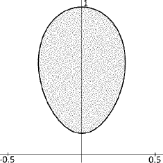
(a) T=0.245

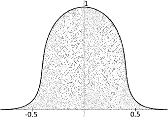
(b) T=0.3

Figure 1. Value ranges $D(T)$

It is easy to see that there are two essentially different cases. In the case of $T\leq\frac{1}{4}$ the set $D(T)$ is a bounded domain with its boundary crossing the imaginary axis at $y=\sqrt{1-4T},\,y=1$. This case corresponds to Theorem 1. If $T>\frac{1}{4}$ the set $D(T)$ is unbounded and its boundary includes the real axis, this case corresponds to Theorem 2. Starting at this point, we only consider the case of $T\leq\tfrac{1}{4}$.

Note that the boundary point $(0,\sqrt{1-4T})$ of $D(T)$ is delivered by the driving function $\lambda(t)\equiv 0$. Therefore, it also belongs to the boundary of $D_{c}(T)$. It is a reasonable assumption that all points of some arc on $\partial D(T)$ near $(0,\sqrt{1-4T})$ are delivered by driving functions with ranges within the interval $[-c,c]$, and since this arc belongs to $\partial D_{c}(T)$. A precise statement is given by the following lemma.

Lemma 2.

A segment of the boundary $\partial D_{c}(T)$ is given by (12), $Y\in[1-4T,Y_{0}]$, $Y_{0}$ is the unique solution of one of the equations

$$2c^{2}\log Y+Y^{2}=1-4T,\,c^{2}\geq T-\frac{1-e^{-4}}{4},$$ (14)

$$\frac{2c^{2}\log Y}{(1+\log Y)^{2}}+Y^{2}=1-4T,\,c^{2}\leq T-\frac{1-e^{-4}}{4}.$$ (15)

Note that if $c^{2}=T-\tfrac{1-e^{-4}}{4}$ both equations (14), (15) have the same root $Y_{0}=e^{-2}$.

Proof.

Consider a point on the boundary $\partial D(T)$. Let $\lambda_{0}(t)$ denote the driving function delivering this point. By Lemma 1 we have $\lambda_{0}(t)=x(t)-p$. Since $p>0$, we can see from (8) that $x(t)$ and, hence, $\lambda_{0}(t)$ are increasing functions.

A boundary point of $D(T)$ belongs to the boundary of $D_{c}(T)$ if it is delivered by a driving function with the range within $[-c,c]$. Since $\lambda_{0}(t)$ is increasing this condition is equivalent to inequalities

$$\lambda_{0}(0)\geq-c,\,\lambda_{0}(T)\leq c.$$ (16)

We note that $\lambda_{0}(0)=-p,\,\lambda_{0}(T)=X-p$. Equations (13) allow us to express $X$ and $p$ through $Y$. Substituting it into (16) and squaring the result we obtain

$$\frac{1-4T-y^{2}}{2\log y}\leq c^{2},\,\frac{1-4T-y^{2}}{2\log y}(1+\log y)^{2}\leq c^{2}.$$

We need to find the greatest value $Y_{0}$ of $Y$ satisfying both conditions. Define the following functions of $Y$ for $Y\in[\sqrt{1-4T},1]$

$$f_{1}(Y)=\frac{1-4T-Y^{2}}{2\log Y},\,f_{2}(Y)=\frac{1-4T-Y^{2}}{2\log Y}(1+\log Y)^{2}.$$

It is easy to see that $f_{1}(Y)\geq f_{2}(Y)$ for $Y\in[e^{-2},1]$, in particular, it is always true if $\sqrt{1-4T}\geq e^{-2}$ or, which is the same, $T-\tfrac{1-e^{-4}}{4}\leq 0$. Therefore, in this case $Y_{0}$ is the solution of $f_{1}(Y)=c^{2}$ which is equivalent to (14) and it remains to prove the case of $\sqrt{1-4T}<e^{-2}$.

We have $f_{1}(Y)\leq f_{2}(Y)$ and the equality sign holds only at $Y=e^{-2}$. Hence, we need to check if $f_{2}$ attains the value $c^{2}$ within the interval $[\sqrt{1-4T},e^{-2}]$. The derivative

$$f_{2}^{\prime}(Y)=\frac{1+\log Y}{2(\log Y)^{2}}(-2Y(1+\log Y)\log Y+\frac{\log Y-1}{Y}(1-4T-Y^{2}))$$

vanishes at $Y=e^{-1}$ and at roots of the equation

$$2\frac{\log Y+1}{\log Y-1}=\frac{1-4T}{Y^{2}}-1.$$

The left-hand side of the equation is an increasing function of $Y$ on $[\sqrt{1-4T},e^{-2}]$ and takes the value $-\tfrac{4}{3}$ at $Y=e^{-2}$, while the right-hand side is decreasing on $[\sqrt{1-4T},e^{-2}]$ and takes the value $\tfrac{1-4T}{e^{-4}}-1>-1$ at $Y=e^{-2}$. Therefore, the derivative $f_{2}^{\prime}$ does not vanish on the interval $[\sqrt{1-4T},e^{-2}]$. Since $f_{2}^{\prime}(\sqrt{1-4T})>0$, $f_{2}$ increases on $[\sqrt{1-4T},e^{-2}]$. Therefore, $f_{2}$ attains its maximum at $Y=e^{-2}$. Hence, $Y_{0}$ is the solution of $f_{2}(Y)=c^{2}$ if the inequality $f_{2}(e^{-2})>c^{2}$ holds. We note that the last inequality gives $c^{2}>T-\frac{1-e^{-4}}{4}$ to complete the proof. ∎

If $\lambda(t)\equiv\pm c$, the phase system (2) can be integrated directly. We need the following properties of its solutions stated by the lemma below.

Lemma 3.

If trajectory $(x(t),y(t))$ satisfies

$$\frac{dx}{dt}=\frac{2(x-a)}{(x-a)^{2}+y^{2}},\,\frac{dy}{dt}=-\frac{2y}{(x-a)^{2}+y^{2}},$$

where $a$ is a real number, then the following quantities are constant

$$(x-a)y,\,(x-a)^{2}-y^{2}-4t.$$

Proof.

The statement can be proved by direct integration of the system. ∎

3. Main Theorem. Now we are ready to prove the following theorem describing the value range $D_{c}(T)$ in the case of $c^{2}\geq T-\frac{1-e^{-4}}{4}$.

Theorem 4.

Let $c^{2}\geq T-\frac{1-e^{-4}}{4}$, $T\leq\frac{1}{4}$ and let curves $l_{1}-l_{4}$ be defined as follows.

1. The curve $l_{1}$ is a segment of the boundary $\partial D(T)$ given by (12), $Y\in[1-4T,Y_{0}]$, $Y_{0}$ is the unique solution of (14).

2. The curve $l_{2}$ is given by solutions $(X,Y)$, $X+iY=z$, $\mu\in[0,1]$ of the equation

$$z^{2}+1-2c(2\mu-1)(z-i)+8\mu c^{2}(\mu-1)\ln\frac{z+c(2\mu-1)}{i+c(2\mu-1)}=4T.$$ (17)

3. The curve $l_{3}$ is given by solutions (X,Y) of the system

$$\left\{\begin{aligned} &2p^{2}\log\frac{Yp}{c}+Y^{2}-p^{2}=1-4T-c^{2},\\ &X=-c+p(1-\log\frac{Yp}{c}),\end{aligned}\right.$$ (18)

where $p\in[c,p_{0}]$ and

$$p_{0}=\sqrt{\frac{1}{2}(\sqrt{(4T+c^{2}-1)^{2}+4c^{2}}+(4T+c^{2}-1))}.$$ (19)

The curve $l_{4}$ is symmetric to $l_{3}$ with respect to the imaginary axis.

If the following equation

$$-4pc+\frac{c^{2}}{p^{2}}\exp{(-\frac{4c}{p})}-p^{2}=1-4T-c^{2}$$ (20)

has two solutions $p_{1}<p_{2}$ in the interval $(c,p_{0})$ we also define curves $l_{5}-l_{10}$.

4. The curve $l_{5}$ is given by solutions (X,Y) of the system (18), $p\in[c,p_{1}]$. The curve $l_{6}$ is symmetric to $l_{5}$ with respect to the imaginary axis.

5. The curve $l_{7}$ is given by solutions (X,Y) of the system

$$\left\{\begin{aligned} &4cp+(X-c)^{2}-Y^{2}-4T=c^{2}-1,\\ &-p\log\frac{(X-c)Y}{c}=2c,\end{aligned}\right.$$ (21)

where $p\in[p_{1},p_{2}]$. The curve $l_{8}$ is symmetric to $l_{7}$ with respect to the imaginary axis.

6. The curve $l_{9}$ is given by solutions (X,Y) of (18), $p\in[p_{2},p_{0}]$. The curve $l_{10}$ is symmetric to $l_{9}$ with respect to the imaginary axis.

The following two cases are possible:

(1) $D_{c}(T)$ is bounded by curves $l_{1},l_{2},l_{5}-l_{10}$, if (20) has two solutions $p_{1}<p_{2}$ in the interval $(c,p_{0})$.

(2) $D_{c}(T)$ is bounded by curves $l_{1}-l_{4}$, if (20) has less than two solutions in the interval $(c,p_{0})$.

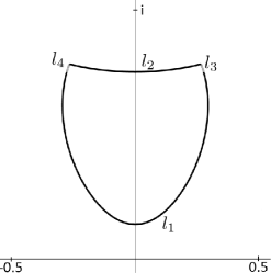
(a) T=0.245, c=1

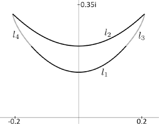
(b) T=0.245, c=0.1

Figure 2. The boundaries of the value ranges $D_{c}(T)$

Proof.

The curve $l_{1}$ is already given by Lemma 2. It can be seen from Lemma 1 that, at $t=0$, the Hamilton function $H$ is maximized at $\lambda_{0}=-p$. Thus, if $p>c$, $H$ attains its maximum on $[-c,c]$ at $\lambda=-c$. Therefore, we have the following driving function:

$$\lambda(t)=\left\{\begin{aligned} &-c,\,&0\leq t\leq t_{1},\\ &x(t)-p,\,&t_{1}<t\leq T.\end{aligned}\right.$$ (22)

Denote $x_{1}=x(t_{1}),\,y_{1}=y(t_{1})$. Applying Lemma 3 to the interval $[0,t_{1}]$ we obtain

$$(x_{1}+c)y_{1}=c,\,(x_{1}+c)^{2}-y_{1}^{2}-4t_{1}=c^{2}-1.$$

Since $\lambda(t)$ is continuous, (22) gives $x_{1}=p-c$. Thus, $y_{1}=\frac{c}{p}$ and we can also find $t_{1}$:

$$4t_{1}=p^{2}-\frac{c^{2}}{p^{2}}-c^{2}+1.$$ (23)

Integration of (6) and (7) over the interval $[t_{1},T]$ yields the system (18). The equation (23) shows that $t_{1}$ increases as a function of $p$. Therefore, we can rewrite the condition $t_{1}\in[0,T]$ as $p\in[c,p_{0}]$, where $c$ and $p_{0}$ are the roots of (23) for $t_{1}=0$ and $t_{1}=T$, respectively. Note that if $p=c$ equations (18) turn into (13).

We have to satisfy the condition $\lambda(t)\in[-c,c]$. Since $\lambda(t)$ is equal to $-c$ on $[0,t_{1}]$ and increases on $[t_{1},T]$, we only have to ensure that $\lambda(T)\leq c$. According to Lemma 2 for $p=c$ we have $\lambda(T)<c$. Assume that at some point $p\in(c,p_{0}]$, $\lambda(T)>c$. Then, due to continuity of $\lambda(T)$ as a function of $p$, there is a point $p_{1}\in(c,p_{0})$, such that $\lambda(T)=c$. Using (22) and (18) we can rewrite it as

$$-p\log\frac{Yp}{c}=2c.$$

With (18) it gives the equation (20) for $p_{1}$. Thus, if (20) has no roots in $(c,p_{0})$ the case (2) takes place. We note, however, the existing of a single root of (20) in $(c,p_{0})$ does not guarantee a violation of the condition $\lambda(T)\leq c$, and, thus, the case (2) is still possible.

Now consider the driving function

$$\lambda(t)=\left\{\begin{aligned} &-c,\,&0\leq t\leq t_{1},\\ &x(t)-p,\,&t_{1}<t\leq t_{2},\\ &c,\,&t_{2}<t\leq T.\end{aligned}\right.$$ (24)

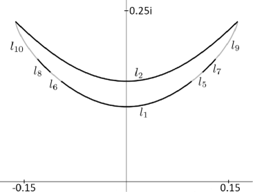
Figure 3. The boundary of the value range $D_{c}(T),T=0.247,c=0.05$

Denote $x_{2}=x(t_{2}),\,y_{2}=y(t_{2})$. Applying Lemma 3 to the phase system for the interval $[t_{2},T]$ we can write

$$(X-c)Y=(x_{2}-c)y_{2},\,(X-C)^{2}-Y^{2}-4T=(x_{2}-c)^{2}-y_{2}^{2}-4t_{2}.$$ (25)

The condition $\lambda(t_{2})=c$ gives $x_{2}=c+p$. Integrating (6) and (7) over the interval $[t_{1},t_{2}]$ we obtain

$$2p^{2}\log\frac{y_{2}p}{c}+y_{2}^{2}-p^{2}=1-4t_{2}-c^{2},\,x_{2}=-c+p(1-\log\frac{y_{2}p}{c}),$$

that with (25) lead us to (21). These equations describe the boundary segment governed by the driving functions of the type (24).

From (25) and (21) we can deduce the equation for $t_{2}$

$$4t_{2}=1-c^{2}+4pc+p^{2}-\frac{(X-c)^{2}Y^{2}}{p^{2}},$$ (26)

and, therefore, we have

$$4(t_{2}-t_{1})=4pc+\frac{c^{2}-(X-c)^{2}Y^{2}}{p^{2}}.$$

The second equation in (21) implies that $c^{2}>(X-c)^{2}Y^{2}$, therefore, the inequality $t_{1}<t_{2}$ always holds. Since $t_{1}$ increases and takes the value $t_{1}=T$ at $p=p_{0}$, there is a point $p_{2}\in[p_{1},p_{0}]$, such that at this point $t_{2}=T$. Substituting $t_{2}=T$ into (26) and using the second equation in (21) we again obtain the equation (20) for $p_{2}$. Thus, we see that existing of two roots of (20) $p_{1}<p_{2}$ in the interval $[c,p_{0}]$ is a necessary condition for the case (1).

It is not difficult to see that the segment of the boundary corresponding to $p\in[p_{2},p_{0}]$ is delivered by the driving functions of the type (22) and, consequently, is described by the system (18).

For the remaining part of the boundary $\partial D_{c}(T)$ the Hamilton function is maximized outside of the interval $[-c,c]$ and, thus, we have $|\lambda(t)|=c$. Therefore, we can use the generalized Loewner equation (see [6, 7])

$$\frac{dg(z,t)}{dt}=\mu\frac{2}{g(z,t)-c}+(1-\mu)\frac{2}{g(z,t)+c},\,g(z,0)=z,\,\mu\in[0,1].$$

Putting $z(t)=g(i,t)$ and integrating the equation over $[0,T]$ we obtain the equation (17) for the curve $l_{2}$, parameterized by $\mu\in[0,1]$. ∎

Acknowledgment. This work was supported by the Russian Science Foundation (project no. 17-11-01229).

References

[1] Goryainov V. V., Gutlyanski V. Ja. On extremal problems in the class . Mat. Sb., Kiev, 1976, pp. 242–-246.
[2] Grunsky H. Neue Abschätzungen zur konformen Abbildung ein- und mehrfach zusammenhängender Bereiche. Schr. Math. Sem. Inst. Angew. Math. Univ. Berl., 1932, vol. 1. pp. 93–-140.
[3] Kager W., Nienhuis B., Kadanoff L. P. Exact Solutions for Loewner Evolutions. J. Stat. Phys., 2004, vol. 115, pp. 805–822. DOI: 10.1023/B:JOSS.0000022380.93241.24.
[4] Koch J., Schleissinger S. Value ranges of univalent self-mappings of the unit disc. J. Math. Anal. Appl., 2016, vol. 433, no. 2, pp. 1772–-1789. DOI: 10.1016/j.jmaa.2015.08.068.
[5] Koch J., Schleissinger S. Three value ranges for symmetric self-mappings of the unit disc. Proc. Amer. Math. Soc., 2017, vol. 145, pp. 1747–1761. DOI: 10.1090/proc/13350.
[6] Prokhorov D. V. Sets of values of systems of functionals in classes of univalent functions. Mat. Sb., 1990, vol. 181, no. 12, pp. 1659–-1677. English translation: Math. USSR Sb., 1992, vol. 71, no. 2, pp. 499-–516.
[7] Prokhorov D. V. Reachable Set Methods in Extremal Problems for Univalent Functions. Saratov Univ., Saratov, 1993.
[8] Prokhorov D. V., Samsonova K. Value range of solutions to the chordal Loewner equation. J. Math. Anal. Appl., 2015, vol. 428, no. 2, pp. 910–-919. DOI: 10.1016/j.jmaa.2015.03.065.
[9] Rogosinski W. Zum Schwarzen Lemma. Jahresber. Dtsch. Math.-Ver., 1934, vol. 44. pp. 258-–261.
[10] Roth O., Schleissinger S. Rogosinski’s lemma for univalent functions, hyperbolic Archimedean spirals and the Loewner equation. Bull. Lond. Math. Soc., 2014, vol. 46, no. 5, pp. 1099-–1109. DOI: 10.1112/blms/bdu054.