The Guided Team-Partitioning Problem: Definition, Complexity, and Algorithm

The Guided TeamPartitioning Problem: Definition, Complexity, and Algorithm

Abstract

A long line of literature has focused on the problem of selecting a team of individuals from a large pool of candidates, such that certain constraints are respected, and a given objective function is maximized. Even though extant research has successfully considered diverse families of objective functions and constraints, one of the most common limitations is the focus on the single-team paradigm. Despite its well-documented applications in multiple domains, this paradigm is not appropriate when the team-builder needs to partition the entire population into multiple teams. Team-partitioning tasks are very common in an educational setting, in which the teacher has to partition the students in her class into teams for collaborative projects. The task also emerges in the context of organizations, when managers need to partition the workforce into teams with specific properties to tackle relevant projects. In this work, we extend the team formation literature by introducing the Guided Team-Partitioning (GTP) problem, which asks for the partitioning of a population into teams such that the centroid of each team is as close as possible to a given target vector. As we describe in detail in our work, this formulation allows the team-builder to control the composition of the produced teams and has natural applications in practical settings. Algorithms for the GTP need to simultaneously consider the composition of multiple non-overlapping teams that compete for the same population of candidates. This makes the problem considerably more challenging than formulations that focus on the optimization of a single team. In fact, we prove that GTP is NP-hard to solve and even to approximate. The complexity of the problem motivates us to consider efficient algorithmic heuristics, which we evaluate via experiments on both real and synthetic datasets.

The input of the general team formation problem consists of a pool of candidates, a set of constraints, and an objective function. The goal is then to strategically select a group of individuals from the pool, such that the group respects all the constraints and also optimizes the objective function. A long line of literature has addressed different versions of the problem that ask for the optimization of functions such as the quality of intra-team communication [24]. Previous work has also considered a diverse array of constraints, such as those on the team’s size [34], the team-builder’s recruitment budget [19], the coverage of a particular set of skills [31], and the workload allocated to each team member [20].

In this paper, we extend the team formation literature by introducing an alternative formulation of the problem that asks for the partitioning of the given pool of candidates into multiple teams, while allowing the team builder to control the properties of each team. We refer to this paradigm as Guided Team-Partitioning (GTP). For instance, consider a teacher who is trying to partition the students in her class into groups, such that the distribution of talent and experience across the groups is balanced [28]. We illustrate an example of this scenario in Figure 1.

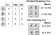
Figure 1: Standard Vs. Fair Clustering

In this example, the input consists of a population of $4$ students $\{A,B,C,D\}$. Each student has a proficiency level for three skills: C++, Algorithms, and Databases. Proficiency is measured on a 1-5 scale, with higher values indicating higher proficiency. The goal is to partition the student population into balanced teams, such as each team has an average proficiency level of $3$ for all three skills. Conceptually, our goal is to avoid teams with an unfair advantage or disadvantage. We refer to $(3,3,3)$ as the target vector, which is used to guide the partitioning task. One approach would be to use a similarity-based clustering algorithm, such as K-means. The best solution would then be to create two clusters $\{A,B\}$ and $\{C,D\}$. The students in the first team would then be highly similar to each other, being experts in C++ and Databases but novices with respect to Algorithms. On the other hand, both $C$ and $D$ have very little knowledge of C++ and are similarly mediocre with respect to the other two skills. Therefore, it is clear that this partitioning fails to approximate the target vector and does not deliver a balanced distribution of talent. If we consider all possible team assignments, it is clear that the best possible option is to create two teams $\{A,C\}$ and $\{B,D\}$ with both having (3, 2, 3.5) as their centroids. The two identical centroids clearly demonstrate the fairness of this partitioning: both teams have an average proficiency of $3,2$, and $3.5$ for C++, Algorithms, and Databases, respectively. In addition, the $(3,2,3.5)$ vector is the closest possible to the ideal $(3,3,3)$ target vector.

This first example captures the scenario in which the centroids of all the teams have to be as close as possible to the same target vector. What if the team builder wants to go beyond this simple balanced partitioning and actually ask for different centroid values for the produced teams? Consider the example shown in Figure 2.

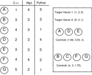
Figure 2: Guided partitioning of a population into teams.

The figure shows a population of 7 students. For each student, we know their proficiency level with respect to C++, Algorithms, and Python, measured on a 1-5 scale. The teacher wants to compare C++ and Python in the context of collaborative projects. In order to achieve this, she needs to partition her 7 students into two teams, such that one team has a high concentration in C++ and a low concentration in Python, while the other team has the exact opposite properties. In addition, both teams need to have a medium concentration in Algorithms, in order to control for the effect of this skill . In the context of the (C++, Algorithms, Python) feature space, the teacher thus specifies the target vectors $(1,3,5)$ and $(5,3,1)$. An exhaustive evaluation of all possible solutions would reveal that the best partitioning would be $(A,D,E)$ and $(B,C,F,G)$. As we show in the picture, the centroids of these two teams are as close to the specified target vectors as possible. This second example demonstrates the main problem that we focus on in our work:

Main Problem: Given a population of individuals, we want to partition the population into teams such that the centroid of each team is as close as possible to a specific target vector.  

In an educational setting, an instructor could use this type of partitioning to create customized training environments by placing students in teams with specific strengths and weaknesses [7, 27]. In general, this type of team partitioning is essential for a team builder who is trying to form and study groups with specific compositions for marketing or experimental purposes [10]. We observe that, even for the toy examples that we presented above, finding the best possible partitioning is a non-trivial task. In addition, the task obviously becomes even more challenging in realistic scenarios with large numbers of candidates and features. In fact, as we show in our work, the problem is NP-hard to solve and even to approximate.

While there exist team formation problems that try to form good teams to cover some skills while minimizing the cost, to the best of our knowledge, our work is the first to tackle this customized team formation problem. Nonetheless, our work has ties to extant research on team formation and other problems, which we review in Section 1. In Section 2, we explore alternative formal definitions and study their hardness. We then present an efficient algorithmic framework in Section 3. In Section 4, we evaluate the efficacy of our framework via an experimental evaluation that includes both real and synthetic data, as well as competitive baselines. Finally, we conclude our work in Section 5.

1 Related Work

Although to best of our knowledge, we are the first to introduce the Guided Team-Partitioning Problem, the nature of our problem is related to semi-supervised clustering and team formation problem. We review only some of these works here:

Semi-supervised Clustering Existing methods for semi-supervised clustering fall into two general approaches constraint-based and metric-based. In constraint-based approaches, the clustering algorithm itself is modified to lead the algorithm towards a more appropriate data partitioning. In order to achieve this, pairwise constraints or user-provided labels are used in the algorithm. This is done by initializing and constraining clustering based on labeled examples  [9], modifying objective function to include constraints [17], or enforcing constraints during the clustering process [33]. In semi-supervised clustering by seeding [9], besides input dataset $\mathcal{R}$ and the number of clusters $k$, given is a subset of the dataset, $S$, in which the cluster they should belong is specified. For all $k$ clusters, there is at least one point in $S$. One of the earliest problems which is close to constraint-based clustering is facility location problem [29] and it is studied mainly in operational research science. It tries to locate $k$ facilities to serve $n$ customers such that the travelling distance from the customers to their facility is minimized. However, the only type of constraints they studied is constraints on the capacity of the facility, i.e., each facility can only serve a limited number of customers. In the work by Bradley et al. [14], $k$ constraints are added to the underlying clustering optimization problem requiring that each cluster has at least a minimum number of points in it. Tung et al. [32] introduces a framework for constraint-based clustering. Their taxonomy of constraints includes constraints on individual objects (e.g. cluster only luxury mansions of value over one million dollars), parameter constraints (e.g. the number of clusters) and constraints on individual clusters that can be described in terms of bounds on aggregate functions (min, avg, etc.). On the contrary, in metric-based approaches, an existent clustering algorithm that uses a distance metric is used; however, the metric is first trained to satisfy the labels or constraints in the given supervised data. Various distance measures have been used for metric-based approaches including but not limited Euclidean distance trained by a shortest-path algorithm [22], Jensen-Shannon divergence trained using gradient descent [16], string-edit distance learned using Expectation Maximization [13], or Mahalanobis distances trained using convex optimization [8].

Team Formation Team formation has been studied in operations research community e.g.  [11], which defines the problem as finding the optimal match between people and demanded functional requirements. It is often solved using techniques such as simulated annealing, branch-and-cut or genetic algorithms e.g.  [11]. Lately it has also been studied in computer science. A majority of these work focus on team formation to complete a task and minimize the communication cost among team members [6]. The focus of these studies is to find only one team to perform a given task. Lappas et al.  [24] introduces the problem of team formation in the context of social networks. Given a pool of experts and a set of skills that needed to be covered, the goal there is to select a team of experts that can collectively cover all the required skills while ensuring efficient intra- team communication. Their work imposes the strong assumption that a single person can fulfill a skill requirement of a task. Whereas a general framework can impose the constraint such that the at least $n$ experts should fulfill the requirements [25]. Bhowmik et al. [12] developed algorithms using submodularity to find teams of experts by relaxing the skill cover requirement such that some skills must be necessarily covered by experts while other skills only improve the team quality. The work by Rangapuram et al. [26] also studies the problem of finding a team of experts based on densest subgraph that is both competent in performing the given task and compatible in working together. The recent work by Anagnostopoulos et al. [2] considers a time-series of arriving tasks whereby users are chosen to finish the arriving tasks without overwhelming any team or any expert, and the team has small communication overhead. A similar study by Kargar et al. [21] considers the problem of finding an affordable and collaborative team from an expert network that minimizes two objectives at the same time: the communication cost among team members and also the personnel cost. Recently, complex task crowdsourcing by team formation has been studied, where the requester wishes to hire a group of workers to work together as a team [35]. In educational settings clustering students into different teams is studied such that students can maximally benefit from peer interaction [4, 5]. In addition, the work by Agrawal et al. [1] considers partitioning students in which each student has only one ability level for all the activities, and each team has a set of leaders and followers in which leaders are helping followers to complete a task. The goal is to maximize the gain of students where the gain is defined as the number of students who can do better by interacting with the higher ability students.

Although all these works focus on identifying good teams, they are different from the work we present here, as most of them focus on finding only one team, or only allow for binary skills, or taking into account only one ability level, or they study very different objective function. In this paper, we introduce a new different optimization function; forming customized teams by placing individuals in teams with specific strengths and weaknesses.

2 Problem Definition

In this section, we begin by describing notational conventions that we will use throughout the paper; then we present the formal statement of the problems that we study. We start from a simple version of our problem with only one team (partition). We show that even the simple version is NP-hard to solve and approximate. Then we move to partitioning problem with desired centroids. In Subsection 2.4, we describe our problem, Guided Team-Partitioning. In the same subsection, we show that our problem is NP-hard to solve and approximate.

2.1 Preliminaries

We consider a pool $\mathcal{R}$ of $n$ individual experts. Each expert ${\mathbf{r}}\in{\mathcal{R}}$ is associated with a ${d}$-dimensional feature (skill) vector ${\mathbf{r}}_{i}$, such that ${\mathbf{r}}_{i}(f)$ returns the value of skill $f$ for expert $i$. We also consider given a set of target vectors $\mathbf{T}$ of $k$ target points $\mathbf{t}$. The goal is to partition the pool of experts into $k$ teams such that the cost of this partitioning is minimized. The cost for each team ${\mathcal{C}}_{i}$, is the distance between the centroid of that team ($\mathbf{mean}$(${\mathcal{C}}_{i}$)) to its target vector ${\mathbf{t}}_{i}$.

$$Cost=\sum\limits_{i=1}^{k}{\mathbf{D}}({\mathbf{mean}}({\mathcal{C}}_{i}),{\mathbf{t}}_{i})$$ (1)

We quantify the closeness between two vectors $\tau$ and $t$ of dimension $d$, using the $L^{2}_{2}$ norm of their difference. We denote this by

$${\mathbf{D}}(\tau,t):=L^{2}_{2}(\tau-t)=\sum\limits_{i=1}^{d}(\tau(i)-τt(i))^{2}$$

We define the $\mathbf{mean}$ of a set $\mathcal{R}$, consisting of $n$ vectors ${\mathbf{r}}_{1},{\mathbf{r}}_{2},\ldots,{\mathbf{r}}_{n}$ as

$${\mathbf{mean}}({\mathcal{R}})=\frac{\sum_{i=1}^{n}{\mathbf{r}}_{i}}{n}$$

2.2 The CIS  Problem

In Characteristic-Item Selection (CIS) problem, the goal is to find a subset of a universe set, such that the mean of the subset is as close as possible to a designated point. This designated point represents the whole set. This intuition is captured in a formal definition as follows.

Problem 1 (CIS).

Given a set ${\mathcal{R}}=\{{\mathbf{r}}_{1},{\mathbf{r}}_{2},\ldots,{\mathbf{r}}_{{n}}\}$, a number ${\mathbf{\ell}}$, and a designated vector ${\mathbf{t}}$, find $\mathbf{\ell}$ points (${\mathcal{R}}_{\mathbf{\ell}}$) to remove from $\mathcal{R}$, such that $\mathbf{mean}$ of the remaining points ${\mathcal{R}}\setminus{\mathcal{R}}_{{\mathbf{\ell}}}$ is close to target $\mathbf{t}$. More formally,

$${\mathbf{D}}({\mathbf{mean}}({\mathcal{R}}\setminus{\mathcal{R}}_{{\mathbf{\ell}}}),{\mathbf{t}})$$

is minimized.

Lemma 1.

The CIS problem is NP-hard to solve and approximate.

Our analysis below demonstrates that the CIS problem is not only NP-hard, but it is also NP-hard to approximate. In order to see this, let’s consider the decision version of the problem which is defined as follows: Given a set ${\mathcal{R}}=\{{\mathbf{r}}_{1},{\mathbf{r}}_{2},\ldots,{\mathbf{r}}_{{n}}\}$, a number $\mathbf{\ell}$, and a designated vector ${\mathbf{t}}$, does there exist a subset ${\mathcal{R}}_{\mathbf{\ell}}\subseteq{\mathcal{R}}$ with $|{\mathcal{R}}_{\mathbf{\ell}}|={\mathbf{\ell}}$ and ${\mathbf{D}}({\mathbf{mean}}({\mathcal{R}}\setminus{\mathcal{R}}_{\mathbf{\ell}}),{\mathbf{t}})\leq q$? We call this decision version of the problem Decision-CIS. The following lemma shows that this problem is NP-complete.

Lemma 2.

The Decision-CIS problem is NP-complete.

Proof.

Without the loss of the generality, we show the NP-completeness of the CIS problem for the case when the elements in ${\mathcal{R}}$ are one-dimensional. We will reduce an instance of the Subset Sum problem to CIS. An instance of Subset Sum problem states that given a universe of $n$ numbers $U=\{x_{1},x_{2},\ldots,x_{n}\}$, does there exist a subset of size $j$ whose sum is $J$? We translate an instance of Subset Sum to CIS by setting ${\mathcal{R}}$ to $U$, ${\mathbf{\ell}}={n}-j$ and ${\mathbf{t}}$ to $\frac{J}{{n}-{\mathbf{\ell}}}$ and $q=0$. We can decide the Subset Sum problem if and only of we can decide for CIS problem.∎

Corollary 1.

The CIS problem is NP-hard and NP-hard to approximate. That is, it is NP-hard to find a polynomial-time approximation algorithm for the CIS problem.

Proof.

We will prove the hardness of approximation of the CIS problem by contradiction. Assume that there exists an $\alpha$-approximation algorithm for the CIS problem. Then if $S^{*}$ is the optimal solution to the problem and $S^{A}$ is the solution output by this approximation algorithm, it will hold that ${\mathbf{D}}({\mathbf{mean}}(S^{A}),{\mathbf{t}})\leq\alpha{\mathbf{D}}({\mathbf{mean}}(S^{*}),{\mathbf{t}}))$. If such an approximation algorithm exists, then this algorithm can be used to decide the decision instances of the CIS  problem for which $q=0$. However, this contradicts the proof of Lemma 2, which indicates that these problems are also NP-hard. Thus, such an approximation algorithm does not exist. ∎

As a use case of this problem, we can name the Characteristic-Review Selection problem (CRS) in [23] which aims to find a small set of reviews from a corpus of reviews for an item, such that the subset presents the whole corpus the best. This is highly useful in on-line shopping and review websites. Consider Tripadvisor; users can rate the characteristics of a hotel such as value, sleep quality, etc. When a user searches for a hotel, she would like to see only an informative subset of reviews which represent all reviews the best and the mean of each feature in the selected subset is as close as possible to the mean of features in the whole set of reviews.

2.3 The CP Problem

Given a set of $n$ workers with different skills and a set of $k$ tasks that need to be done collaboratively with given average required skill levels for each task, the goal is to form teams of workers that their mean skill level matches each task the best. This team formation problem can be considered as one of the applications of the ${\sc CP}$ (Characteristic Partitioning) problem which is formally defined in the following problem

Problem 2 (CP).

Given a set ${\mathcal{R}}=\{{\mathbf{r}}_{1},{\mathbf{r}}_{2},\ldots,{\mathbf{r}}_{{n}}\}$ and target vectors ${\mathbf{T}}=\{{\mathbf{t}}_{1},{\mathbf{t}}_{2},\ldots,{\mathbf{t}}_{{k}}\}$, partition ${\mathcal{R}}$ into ${k}$ partitions ${\mathcal{C}}_{1},{\mathcal{C}}_{2},\ldots,{\mathcal{C}}_{k}$ such that

$$\sum\limits_{i=1}^{k}{\mathbf{D}}({\mathbf{mean}}({\mathcal{C}}_{i}),{\mathbf{t}}_{i})$$

is minimized.

Corollary 2.

The CP problem is NP-hard to solve and NP-hard to approximate.

Proof.

We will reduce an instance of Subset Sum problem to CP problem, by setting $k$=2 and ${\mathbf{t}}_{1}=\frac{J}{j}$. Thus if Cluster 1 has exactly $j$ points which the mean of points is $\frac{J}{j}$, the sum of elements in cluster 1 would be equal to $J$. Without loss of generality let’s assume for all ${\mathbf{r}}_{i}\in{\mathcal{R}}$, $0\leq{\mathbf{r}}_{i}\leq v$. Now we can add an extra point ${\mathbf{r}}_{n+1}$ such that $v\ll{\mathbf{r}}_{n+1}$. Now we can set ${\mathbf{t}}_{2}=\frac{{\mathbf{r}}_{n+1}+Sum({\mathcal{R}})-J}{{n}-j+1}$. In order to minimize the cost of CP problem, there should be ${n}-j$ elements of $\mathcal{R}$ and ${\mathbf{r}}_{n+1}$ in cluster 2 and hence $j$ elements in Cluster 1. ∎

2.4 The Guided Team-Partitioning Problem

For many applications, it is not necessary to assign all the points in the dataset to teams. For instance, when separating a workforce into teams so that each team has a specific level of expertise in each skill, it is acceptable to exclude some of the workers. In general, having the option to exclude up to a fixed number of points adds flexibility and can only make the problem easier to solve. We capture this intuition in a formal problem definition as follows.

Problem 3 (Guided Team-Partitioning).

Given a set ${\mathcal{R}}=\{{\mathbf{r}}_{1},{\mathbf{r}}_{2},\ldots,{\mathbf{r}}_{{n}}\}$, and target vectors ${\mathbf{T}}=\{{\mathbf{t}}_{1},{\mathbf{t}}_{2},\ldots,{\mathbf{t}}_{{k}}\}$, and a budget ${\mathbf{\ell}}$, find ${\mathbf{\ell}}$ points (${\mathcal{R}}_{\mathbf{\ell}}$) to remove from the dataset and partition the rest of the points ${\mathcal{R}}\setminus{\mathcal{R}}_{{\mathbf{\ell}}}$ into ${k}$ partitions ${\mathcal{C}}_{1},{\mathcal{C}}_{2},\ldots,{\mathcal{C}}_{k}$ such that Cost =

$$\sum\limits_{i=1}^{k}{\mathbf{D}}({\mathbf{mean}}({\mathcal{C}}_{i}),{\mathbf{t}}_{i})$$

is minimized.

Corollary 3.

The Guided Team-Partitioning problem is NP-hard to solve and NP-hard to approximate.

This problem is clearly NP-hard, as it contains the CP problem as a special case (for ${\mathbf{\ell}}=0$).

So far we have discussed the Guided Team-Partitioning problem. For a collection of workers $\mathcal{R}$ in which each worker has a proficiency level for each skill, the most natural translation of the target vectors is the mean of the proficiencies or the required skills of a given project. For instance, consider online labor markets such as Freelancer (www.freelancer.com), Guru (www.guru.com), and oDesk (www.odesk.com) where employers hire freelancers with specific skills to work on different types of projects. The required skills listed for each project in these platforms can be used as the target vectors. In such a setting, each team should poses a specific share of expertise across all skills that makes the team capable of finishing a particular task or project.

Discussion: As a natural result of our objective function, as the number of partitions grows, the cost increase as well. In some applications, target vectors are not given, and in such a setting the goal is to form fair teams with the same level of proficiencies. An example is partitioning the students into teams with the same abilities. If ${k}$ is not predetermined either, finding the right ${k}$ might not be easy due to the fact that as ${k}$ increases, the cost may increase as well. In this situation, we are not able to increase the number of partitions ${k}$, and stop when the cost is not improved. To overcome this, one can redefine the cost as the following:

$$\sum\limits_{i=1}^{k}{\mathbf{D}}({\mathbf{mean}}({\mathcal{C}}_{i}),{\mathbf{t}}_{i})*|C_{i}|$$

3 Algorithm

In this section, we describe GuidedSplit; it finds an efficient solution for Guided Team-Partitioning. We start by presenting algorithms to solve CIS and CP problem and then we use these algorithms to solve Guided Team-Partitioning problem.

3.1 Solving The CIS Problem

Although CIS  problem is NP-hard to solve and approximate, we propose two heuristic algorithms that work well in practice.

The Greedy Algorithm: The Greedy algorithm is an iterative algorithm to solve CIS problem. At each iteration, the algorithm selects a point to remove from data, such that it decrease the distance of $\mathbf{t}$ from the mean of remaining points. The pseudocode of the Greedy algorithm is shown in Algorithm 1.

1:Input: Input set $\mathcal{R}$, target vector $\mathbf{t}$ and number of points to be removed $\mathbf{\ell}$

2:Output: A subset ${\mathcal{R}}_{{\mathbf{\ell}}}$ such that $|{\mathcal{R}}_{{\mathbf{\ell}}}|={\mathbf{\ell}}$

3:${\mathcal{R}}_{{\mathbf{\ell}}}=\{\}$

4:for  $i=1\ldots{\mathbf{\ell}}$ do

5:    ${\mathbf{r}}=argmin_{{\mathbf{r}}^{\prime}\in{\mathcal{R}}}({\mathbf{D}}({\mathbf{mean}}({\mathcal{R}}\setminus\{{\mathbf{r}}^{\prime}\}),{\mathbf{t}})))$

6:    ${\mathcal{R}}_{{\mathbf{\ell}}}={\mathcal{R}}_{{\mathbf{\ell}}}\bigcup\{{\mathbf{r}}\}$

7:    ${\mathcal{R}}={\mathcal{R}}\setminus\{{\mathbf{r}}\}$

8:return ${\mathcal{R}}_{{\mathbf{\ell}}}$

Algorithm 1 The Greedy Algorithm

The algorithm works as the follows, at each iteration in Line 4, a point is selected to be removed from the set of remaining points such that the mean of the remaining points will be close to target $\mathbf{t}$. For a collection $\mathcal{R}$ of $n$ items, the running time of the Greedy algorithm is $O({\mathbf{\ell}}{n}T_{d})$ where $\mathbf{\ell}$ is the number of points to be removed from input data and $T_{d}$ is the time required to compute the distance $\mathbf{D}$ in line 5 of the algorithm. In our case, we used euclidean distance and therefore this time is $O({d})$ (number of dimensions). Thus the running of the Greedy algorithm is $O({\mathbf{\ell}}{n}{d})$. Although the Greedy algorithms is a simple and fast solution to CIS problem; but in practice, it doesn’t perform well. Therefore we propose another solution, ConvexOpt algorithm, which is presented next.

The ConvexOpt Algorithm: We can formulate CIS  problem as a Mixed Integer optimization problem to find a binary vector $x$ such that ${\mathbf{mean}}({\mathcal{R}}x)={\mathbf{t}}$ subject to $\sum\limits_{i=1}^{n}x={n}-{\mathbf{\ell}}$. Since solving mixed integer problem is NP-hard and would require complex algorithms to solve, we instead relax this problem to a convex quadratic programming by removing the binary constraints as shown in Algorithm 2. This ConvexOpt algorithm forms a nonnegative real-valued vector $x$ such that ${\mathbf{D}}({\mathbf{t}},{\mathbf{mean}}({\mathcal{R}}x))$ (Line 3) is small. Note that the aim is to find a subset $\mathbf{S}$ of length ${n}-{\mathbf{\ell}}$ such that ${\mathbf{mean}}({\mathbf{S}})$ is close to $\mathbf{t}$, in another word ideally, we want ${n}-{\mathbf{\ell}}$ elements of $x$ to be equal $\frac{1}{({n}-{\mathbf{\ell}})}$, and the rest be 0 (and ${\mathcal{R}}x={\mathbf{t}}$). This constraint is implied in Line 6 and 5. The algorithm tries to find a vector $x$ of real values such that its elements are between 0 and 1 and the sum of elements of x is at least ${n}-{\mathbf{\ell}}$. Then we transform this real-valued vector to a binary vector by replacing the $n-{\mathbf{\ell}}$ largest elements to 1 and the rest to 0. We used CVX package in Matlab to solve this convex quadratic programming.

1:Input: Input set $\mathcal{R}$, target vector $\mathbf{t}$ and number of points to be removed $\mathbf{\ell}$

2:Output: A subset ${\mathbf{S}}$ such that $|{\mathbf{S}}|=n-{\mathbf{\ell}}$

3:    minimize $\mathbf{D}$(${\mathcal{R}}*x*\frac{1}{n-{\mathbf{\ell}}},t^{\prime}$)

4:    subject to     

5:       sum($x$) $\geq n-{\mathbf{\ell}}$

6:       $x\geq 0$ and $x\leq 1$ and $x\in\mathbb{R}$     

7:Set $n-{\mathbf{\ell}}$ largest values of $x$ to 1 and the rest to 0

8:return ${\mathbf{S}}={\mathcal{R}}(x)$

Algorithm 2 The ConvexOpt  Algorithm

3.2 Solving CP Problem

Our algorithm for the CP problem, which we call the Max Benefit algorithm, is a polynomial time algorithm that finds a partitioning of data points $\mathcal{R}$, into $k$ partitions. The pseudocode of the Max Benefit algorithm is shown in Algorithm 3.

1:Input: Input set $\mathcal{R}$, target vectors $\mathbf{T}$ and number of partitions $k$

2:Output: Partitions $\mathcal{C}$

3:${\mathcal{C}}=\{\}$

4:for $\mathbf{r}$ in $\mathcal{R}$ do

5:    $j=argmax_{i=1\ldots{k}}({\mathbf{D}}({\mathbf{t}}_{i},{\mathbf{mean}}({\mathcal{C}}_{i}))-{\mathbf{D}}({\mathbf{t}}_{i},{\mathbf{mean}}({\mathcal{C}}_{i}\bigcup{{\mathbf{r}}})))$

6:    Add $\mathbf{r}$ to partition $j$, ${\mathcal{C}}_{j}$

7:while no convergence achieved do

8:    for $\mathbf{r}$ in $\mathcal{R}$ do

9:       $h=\text{ The partition }{\mathbf{r}}\text{ belongs to}$

10:       $loss={\mathbf{D}}({\mathbf{t}}_{h},mean({\mathcal{C}}_{h}\setminus\{{\mathbf{r}}\}))-{\mathbf{D}}({\mathbf{t}}_{h},mean({\mathcal{C}}_{h}))$

11:       $j=argmax_{i=1\ldots{k}}(loss+{\mathbf{D}}({\mathbf{t}}_{i},{\mathbf{mean}}({\mathcal{C}}_{i}))-{\mathbf{D}}({\mathbf{t}}_{i},{\mathbf{mean}}({\mathcal{C}}_{i}\bigcup\{{\mathbf{r}}\})))$

12:       Remove $\mathbf{r}$ from partition $h$ and update ${\mathbf{mean}}({\mathcal{C}}_{h})$

13:       Add $\mathbf{r}$ to partition $j$ and update ${\mathbf{mean}}({\mathcal{C}}_{j})$     

14:Return $\mathcal{C}$

Algorithm 3 The Max Benefit  Algorithm

The algorithm works as follows. First, the input data is partitioned into $k$ partitions in Line 3 to Line 6. The decision to assign a point to partition $j$ is made on Line 5 based on how much that point makes the mean of the partition closer to the target point of that partition. Then after initial partitions are formed, points are reassigned in Line 7 to Line 13 . For each point, the benefit of assigning it to other partitions is computed. This benefit is defined as the gain of assigning that point to other partitions + the loss of removing it from its own partition (Line 11). The process is repeated till the solution stabilizes and there is no more improvement in the cost. In practice, the solution stabilized in a few iterations. The running of time of each iteration of Algorithm 3 is $O({n}{k}d)$ in which $d$ is the number of dimensions (for input data $\mathcal{R}$, and targets $\mathbf{t}$).

Discussion: It may seem that instead of using Algorithm 3, we can assign each point to its closest target. To see why this algorithm doesn’t work, consider three data points $a=(1,0)$, $b=(-1,0)$, $c=(-1,20)$, and two target vectors $t_{1}=(0,0)$ and $t_{2}=(-1,10)$. If each point is assigned to the closest target, the first partition includes $a$ and $b$ and the second partition only includes $c$. In this case, the centroids of the partitions are $(0,0)$ and $(-1,20)$ respectively. On the other hand, our proposed algorithm assigns $a$ to the first partition and $b$ and $c$ to the second partition with centroids as $(1,0)$ and $(-1,10)$ which clearly has a lower cost.

3.3 Solving the Guided Team-Partitioning Problem

Let’s assume we are given $k$ partitions (such that mean of each partition ${\mathcal{C}}_{i}$ is close to ${\mathbf{t}}_{i}$) and along with each partition, we are given $q$ points (for all $q=1\ldots{\mathbf{\ell}}$) to be removed from that partition. Now we can develop a dynamic programming algorithm to optimally identify $\mathbf{\ell}$ points to be removed from all partitions. Let $B(i,q)$ denote the benefit of removing the given $q$ points from the $i^{th}$ partition. The benefit is defined as how much the mean of a partition will get closer to its designated target. More formally the benefit of removing points ${\mathcal{R}}_{q}$ from partition ${\mathcal{C}}_{i}$ with target ${\mathbf{t}}_{i}$ is ${\mathbf{D}}(mean({\mathcal{C}}_{i}),t_{i})-{\mathbf{D}}(mean({\mathcal{C}}_{i}\setminus{\mathcal{R}}_{q}),t_{i})$. Let also $MBR(i-1,j-q)$ denote the benefit of removing $j-q$ points from partitions $1^{st}$ to $(i-1)^{th}$ partitions. The final goal is to find the $MBR({k},{\mathbf{\ell}})$, the benefit of optimally removing ${\mathbf{\ell}}$ points from first to last (${k}^{th})$ partition. The following dynamic programming shows how we decide upon removing points from partitions optimally.

$$MBR(i,j)=\max\limits_{0\leq q\leq j}\{MBR(i-1,j-q)+B(i,q)\}$$

At this stage, we have the tool to remove $\mathbf{\ell}$ points from all partitions. Now we can use Algorithm 3 to find the partitions $\mathcal{C}$ and using Algorithm 2, we can find the $q$ points to be removed from each partition. Putting everything together, we end up with Algorithm 4 which is an efficient solution to the Guided Team-Partitioning problem. We call this algorithm GuidedSplit.

1:Input: Input set $\mathcal{R}$, target vectors $\mathbf{T}$, number of partitions $k$ and number of points to be removed $\mathbf{\ell}$

2:Output: Partitions $\mathcal{C}$

3:$\mathcal{C}$= Partition $\mathcal{R}$ into $k$ parts using Algorithm 3

4:for ${\mathcal{C}}_{i}$ in $\mathcal{C}$ do

5:    for $j=1\ldots{\mathbf{\ell}}$ do

6:       $B(i,j)$ = Benefit of removing $j$ points from partition $p_{i}$ using Algorithm 2     

7:for $i=1\ldots{k}$ do

8:    for $j=1\ldots{\mathbf{\ell}}$ do

9:       $MBR(i,j)=\max\limits_{0\leq q\leq j}\{MBR(i-1,j-q)+B(i,q)\}$     

10:return $MBR({k},{\mathbf{\ell}})$ and remove corresponding ${\mathbf{\ell}}$ from partitions

Algorithm 4 The GuidedSplit  Algorithm

The algorithm works as follows: First, the data is partitioned into $k$ partitions such that the mean of each partition is close to its target point in Line 3. Then for each partition, the $j$ ($j=1\ldots{\mathbf{\ell}}$) points that can be removed from that partition is obtained in Line 4 to Line 6, and the benefit of removing each $j$ point from each partition is kept in the matrix $B$. Finally, with a dynamic programming in Line 10 it is decided which ${\mathbf{\ell}}$ points should be removed from all partitions. Note that in the algorithm instead of using Algorithm 2 at Line 6, we can also use the Greedy algorithm, although the Greedy algorithm runs faster, but Algorithm 2 outperforms the Greedy algorithm.

Running time of step 1 (Line 3) is $O({n}{k}d)$. Step 2 (Line 4 to Line 6) involves solving ${k}{\mathbf{\ell}}$ quadratic programming. In theory, the convex quadratic programming can be solved in the cubic number of variables [36]. Thus the overall running time of step 2 is $O({k}{\mathbf{\ell}}{n}^{3})$. We have used the Infeasible path-following algorithm to solve convex quadratic programming which in practice runs much faster than $O({n}^{3})$. Finally, the dynamic programming will take $O({k}{\mathbf{\ell}}^{2})$. Therefore the overall running time of Algorithm 4 is $O({k}{\mathbf{\ell}}{n}^{3})$. In practice, our algorithm tends to have partitions of almost the same size and hence number of data points in each partition is almost $\frac{{n}}{{k}}$. This means our algorithm runs in $O(\frac{{\mathbf{\ell}}{n}^{3}}{{k}^{2}})$ in practice. Note that Step 2 in Algorithm 4 can be executed in parallel for all partitions and all values of $j$.

4 Experiments

In this section, we evaluate our algorithmic solution to the Guided Team-Partitioning problem. Our datasets and implementation are immediately and freely available for download. We begin with a description of the datasets and baseline algorithms, followed by a detailed description of each experiment.

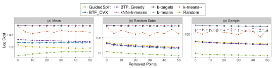
Figure 3: Different algorithms on Skills dataset with respect to increasing $\mathbf{\ell}$. The fixed parameters are $k$ = 5, $n$ = 500 and $d$ = 10.

4.1 Datasets

We next describe the datasets that we used in our experiments.

• The Skills dataset consists of the skill sets of 14960 LinkedIn users who have listed at least one data science role in their profiles. We only keep the 40 most frequent skills in the dataset. Each user is thus represented by a vector of length 40, which contains the number of endorsements she has received for each skill from fellow LinkedIn users.

• The BIA dataset is collected from entry surveys taken by all students who take the Analytics course offered by one of the authors of this paper. The data was collected during 6 different semesters and includes 502 students. For each student, the dataset includes a self-assessment of her level of expertise with respect to machine learning, analytics, programming, and experience with team projects. The assessments are given on a scale from 0 (no experience) to 3 (very experienced).

• The Guru  dataset consists of 6473 experts and 1764 projects from www.guru.com. While the majority of projects in Guru require up to 10 skills, larger projects of 30 skills or more are also posted. The dataset also includes the skills required by the projects, which we use to populate the target vectors. Both the target vectors and the expert skill sets are binary. If an expert possesses a particular skill (or a project requires that skill), the value for that skills is set to 1, otherwise to 0.

• The Freelancer dataset contains 1763 experts and 721 projects from www.freelancer.com. On the Freelancer platform, employers are only allowed to specify at most 5 skills per project. Hence, for each project in our dataset, we have a vector in which the value of the five listed skills are set to 1 and the rest to 0. For each expert and each skill they possess, we have a percentage, such that the sum of skill percentages for each expert is equal to 1.

• The Synthetic dataset is used to generate a ground truth benchmark for our evaluation. We generate the synthetic data as follows. Let $k$ be the number of partitions, $m$ the number of data points per partition, $\mathbf{\ell}$ the number of noisy points added to the data (and should be removed by an effective algorithm), $d$ the number of dimensions, and $\mathbf{\sigma}$ the sampling error (standard deviation). In order to generate synthetic data, we first create $k$ target vectors by sampling from the $[0,1]^{d}$ value space. Then, using each target vector, we generate $m$ data points from a normal distribution with $\mu={\mathbf{t}}_{i}$ and $\mathbf{\sigma}$. Finally, we add $\mathbf{\ell}$ noisy instances by sampling uniformly from $[0,1]^{d}$.

4.2 Methods For Generating the Target Vectors

For experiments on the Guru and Freelancer datasets, we use the skills required by the projects to populate the target vectors. The other datasets, however, do no include a resource that we can intuitively use for the same purpose. We address this by considering three different methods for generating the target vectors: Random-Sobol, Mean, and Sampling. The Mean method sets the target vector equal to the average value of all the points in the dataset. The Sample method randomly selects points from the dataset to serve as the target vectors. The Random-Sobol method uses the concept of the Sobol Sequence [30] to generate targets with $d$ features. When using a standard uniform random generator, it is possible for all or many of the samples values to fall within a specific pocket of the sampling space coincidentally. Quasi-random sequences like the Sobol Sequence address this issue, as their output is constrained in order to lead to low-discrepancy samples. This is achieved by introducing a correlation between the samples (i.e., the generation of a sample considers the values of all the previous samples), which ensures that the sample values are more evenly spread.

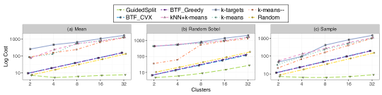
Figure 4: Different algorithms on Skills dataset with respect to increasing $k$. The fixed parameters are $n$ = 500, $\mathbf{\ell}$ = 50 and $d$ = 10.

4.3 Baseline Algorithms

Next, we describe the baseline algorithms that we compare against our own method.

• Random: Random randomly assigns points to partitions.

• k_means: k_means is a clustering method used to minimize the average squared distance between the points in the same cluster.

• k_targets: k_targets is similar to k_means  with the exception that we used the target vectors to initialize the cluster centers. The motivation is to help the algorithm converge to a good solution, given its well-documented sensitivity to the initial seed centers [3].

• k_means–: k_means–  [15] is a generalization of the k_means optimization problem, which tries to cluster the data and discovering the outliers simultaneously. Therefore, the delivered solution consists of $k$ clusters and $\mathbf{\ell}$ outliers.

• kNN+k_means: In this approach, we computed the nearest neighbors of each point and removed $\mathbf{\ell}$ data points with the largest distance to their nearest neighbors. After removing these $\mathbf{\ell}$ points, we run k_means  on the remaining data points and get $k$ partitions.

• BTF_CVX and BTF_Greedy: Best Team First is a family of algorithms that work iteratively, and at each iteration creates the best team from the remaining available users. This is a popular technique [2, 1] that clearly does a excellent job of maximizing the quality of the first group. However; the quality for the subsequent teams can decrease considerably. We take a similar approach here, and at each time we select a team of size $\frac{{n}-{\mathbf{\ell}}}{{k}}$ from the remaining data points. To select a team of a particular size at each iteration, we use ConvexOpt and Greedy  algorithm where at each iteration, $\mathcal{R}$ is the set of remaining data points and the number of points to be removed is the number of remaining data points - $\frac{{n}-{\mathbf{\ell}}}{{k}}$. We call these baselines BTF_CVX and BTF_Greedy respectively.

After obtaining the partitions using Random, k_means, k_targets, k_means–, and kNN+k_means  approaches, we need to find a correspondence between each partition and each target vector. The task of assigning partitions to specific target vectors is an instance of assignment problem. The input to the problem includes two sets of equal sizes, $\mathbf{T}$ (given targets) and $\mathbf{C}$ (obtained partition centers), and a weight function ${\mathbf{D}}:{\mathbf{T}}\times{\mathbf{C}}\rightarrow R$. The goal is to find a bijection $\pi:{\mathbf{C}}\rightarrow{\mathbf{T}}$, such that the cost function $\sum_{a\in{\mathbf{C}}}{\mathbf{D}}(a,\pi(a))$ is minimized. We can complete this task via The Hungarian algorithm [18], which solves the assignment problem optimally in $O({k}^{3})$, where $|{\mathbf{C}}|=|{\mathbf{T}}|={k}$. Thus, after obtaining the partitions, we use the Hungarian algorithm to match the obtained partition centers to the given targets.

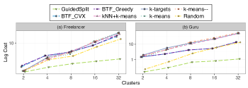
Figure 5: Different algorithms on Freelancer, and Guru datasets.

4.4 Experimental Evaluation

Having all the datasets and target vectors ready as the input of Problem 3, we compare the efficacy of GuidedSplit algorithm with the baseline algorithms. We implemented our algorithm in Matlab and used CVX package to solve the convex optimization problem in the ConvexOpt algorithm. All experiments were carried out on a machine with a 2.4 GHZ CPU, 16 GB RAM, running CentOS Linux 7. We repeated each experiment 25 times and reported the average. The confidence intervals were very tight, and we thus omit them from the plots. We compare the cost of our algorithm compare to all other baselines. This cost refers to the distance from the mean of each partition to its target vector, see equation 1. What follows is the detailed description of each experiment.

4.4.1 Effectiveness with respect to number of discarded points $\mathbf{\ell}$

The goal of this experiment is to demonstrate how different algorithms behave with respect to the number of removed points $\mathbf{\ell}$, as presented in the definition of Problem 3. In this experiment we set number of data points to 500, number of partitions to 5, number of dimensions to 10 ($k$ = 5, $n$ = 500 and $d$ = 10). We report the results of all three different methods of choosing the target vectors ( Random-Sobol, Mean, and Sampling methods). Figure 3 shows the cost (in log scale) versus $\mathbf{\ell}$.

We observe that our GuidedSplit  algorithm consistently outperforms the baseline algorithms for all target vectors, and the cost of GuidedSplit is significantly less than all the baselines. We also observe when all the targets are set to the mean, the Random algorithm is doing well. This is simply because a random sample of the data is expected to have the same mean as the whole data.

An interesting observation is that when targets are equal to the mean of the dataset, Figure 3(a), as $\mathbf{\ell}$ increases the cost of GuidedSplit increases as well. The reason is after finding partitions when $\mathbf{\ell}$ = 0, GuidedSplit finds near perfect solution in which mean of each partition is very close to its target. Removing points from the partition discomposes the obtained solution and makes the mean of partition far from its target. We also tried this experiment on other datasets; the results were similar, and GuidedSplit outperforms in those experiments as well. However, the algorithms were more competitive on Skills dataset. Thus due to lack of space, we only report results on Skills dataset.

4.4.2 Effectiveness with respect to number of partitions $k$

The goal of this experiment is to demonstrate how the algorithms behave with respect to the number of partitions $k$. In these experiments, we show the cost (in log scale) versus different number of partitions ($k$ = 2, 4, 8, 16, 32) and we fixed $n$ = 500, $\mathbf{\ell}$ = 50 and $d$ = 10 on Skills dataset and $n$ = 502, $d$ =4 and $\mathbf{\ell}$ = 50 for BIA dataset. In the experiment on BIA dataset, to form fair teams of students with an equal level of expertise, the targets of partitions are set to be equal to the mean of the whole dataset. We present the results in Figure 4(a), Figure 4(b), and Figure 4(c) for all three different methods of choosing the target vectors ( Random-Sobol, Mean, and Sampling methods) on Skills dataset and Figure 6 depicts the results on BIA dataset.

As observed before, our GuidedSplit  algorithm consistently outperforms the baselines for all target vectors, and the cost of GuidedSplit is significantly less than all the baselines. Note that as the objective function here is to minimize the distance of targets to the mean of partitions, cost increases with the number of partitions. But GuidedSplit  is still able to find efficient partitions compared to all baselines, and its cost does not increase dramatically.

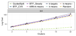
Figure 6: Different algorithms on BIA  dataset with respect to increasing $k$. The fixed parameters are $n$ = 502, $\mathbf{\ell}$ = 50, and $d$ = 4.

4.4.3 Results on the Freelancer and Guru datasets

Guru and Freelancer datasets have a different dynamic compare to other datasets. In these datasets, we can use the required skills of the projects as the target vectors. Besides, the projects posted in freelancer and guru, are the tasks that require a few skills and they can also be completed by a small team of experts. So we conducted an experiment specifically for these two datasets which indicates the performance of our algorithm with respect to the number of points $n$, the number of partitions $k$, and the number of points to remove $\mathbf{\ell}$.

For this experiment, we used the set of experts as input set $\mathcal{R}$, and the projects as target vectors $\mathbf{T}$. We tried $k$ =2, 4, 8, 16, 32, and for each value of $k$, we used $k$  projects at random. We also set $n$ = $k$ * 5 and $\mathbf{\ell}$ = $k$ (and selected $n$ + $\mathbf{\ell}$ experts as random as the input $\mathcal{R}$). The intuition behind is due to the inherent nature of projects posted in Guru and Freelancer; these projects are small projects that usually do not need more than 5 people to be completed. By setting $n$= $k$ * 5 and $\mathbf{\ell}$ = $k$, ideally, the size of each team would be 4. The results in Figure 5(a) and 5(b) illustrate GuidedSplit  algorithm outperforms baseline algorithms on Freelancer and Guru datasets, and find teams of experts whose proficiencies are close to required skills of projects.

4.4.4 Effectiveness with respect to population size $n$

We also experiment how different algorithms behave with respect to the number of points $n$, for $n$ =100, 500, 1000, 2500, 5000, 10000. In this experiment, we show the cost (in log scale) versus population size, $n$on the Synthetic dataset, where the fixed parameters are $k$ = 5, $\mathbf{\ell}$ = 50, and $d$ = 10. The result is depicted in figure 7.

The results illustrate that GuidedSplit is capable of forming the right clusters with the hidden structures as was imposed by the Synthetic dataset. As explained before, the Synthetic dataset has a distinct structure; each cluster has a different mean, and this structure is very easy for k_means  and k_targets algorithms to find. This is also the reason Random  performance degrades; because it cannot find the hidden structure of the data.

In addition, We also examined the points removed by our algorithm; we observed that majority of removed points are exactly the noisy points we added to the data (the points randomly sampled from $[0,1]^{d}$ space). We also tried this experiment on other datasets; the results were similar. However, the algorithms were more competitive on Synthetic dataset compare to other datasets. Thus we only report results on the Synthetic dataset, and we leave out the results on other datasets.

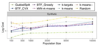
Figure 7: Different algorithms on Synthetic dataset with respect to increasing $n$. The fixed parameters are $k$ = 5, $\mathbf{\ell}$ = 50, and $d$ = 10.

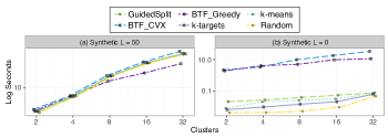
Figure 8: Running time of algorithms with respect to number of clusters.

4.4.5 Running Times

We only show the running time for the top six competitive algorithms which performed well in experiments on real datasets and used the ConvexOpt or the Greedy algorithm. We exclude k_means– and kNN+k_means in this experiments since they do not need to use the ConvexOpt or the Greedy algorithm and thus their running times are less than the other algorithms. Clearly as illustrated in preceding experiments, the performance of k_means–, and kNN+k_means are not comparable to other algorithms either.

We report the running time on the Synthetic dataset when increasing the number of partitions $k$  where other parameters are $n$ = 500, $\mathbf{\sigma}$ = 0.2 $\mathbf{\ell}$ = 50. We also report the same experiment when $\mathbf{\ell}$ = 0. Naturally when $\mathbf{\ell}$ = 0, algorithms run faster since they do not need to execute ConvexOpt algorithm. This means the running time of GuidedSplit algorithm only includes of running Line 3 in Algorithm 4. We also report the running time versus population size $n$ where fixed parameters are $k$ = 5, $\mathbf{\sigma}$ = 0.2 and for both $\mathbf{\ell}$ = 0 and $\mathbf{\ell}$ = 50.

Figure 8(a) shows the runtime in log seconds versus increasing the number of clusters where fixed parameters are $n$5̄00 and $\mathbf{\ell}$ = 50, and $\mathbf{\sigma}$ = 0.2 . As mentioned in subsection 3.3, the running time of our GuidedSplit algorithm is mainly bounded by Line 4 to Line 6 in Algorithm 4, where $j$ (for $j=1\ldots{\mathbf{\ell}}$) points are removed from each cluster. This also applies to Random, k_means, and k_targets since they also use the same algorithm to remove $\mathbf{\ell}$ points. The running time of Line 4 to Line 6 is $time(\text{removing }{\mathbf{\ell}}^{2})*{k}$. In theory $time(\text{removing }{\mathbf{\ell}})$ is $O(n^{3})$ which $n$ is the number of points in each cluster. In consequence, as the number of clusters increases, Guided Team-Partitioning needs to remove ${\mathbf{\ell}}^{2}$ points for more clusters and hence the running time also increases.

Note that Random, k_means, and k_targets require an extra step in which after clustering is done, the center of each cluster is matched with one of the targets using Hungarian algorithm. The running of this step only depends on the number of clusters. Figure 8(b) shows the running time of the algorithms when $\mathbf{\ell}$ = 0; hence there is no need to run ConvexOpt algorithm (except for BTF_CVX baseline) and the reported running time only includes clustering and using Hungarian algorithm to match the cluster centers to targets. As an interesting result, the running time of BTF_CVX and BTF_Greedy is considerably higher than other algorithms even though $\mathbf{\ell}$ = 0 and this is due the fact that for the BTF_CVX (BTF_Greedy) algorithm we need to run the ConvexOpt (Greedy) algorithm $n$  times.

Figure 9(a) shows the runtime in log seconds versus increasing the number of points in the data, where $k$ = 5 and $\mathbf{\ell}$ = 50, and $\mathbf{\sigma}$ = 0.2. The reason Random has the minimum running time is that it creates very balanced clustering in which the number of points in all clusters are very similar. This means when removing the points, the running time of Line 4 to Line 6 in Algorithm 4 is almost ${k}*(\frac{{n}}{{k}})^{3}$ which is considerably smaller in the case that there is one very large cluster and the rest of clusters have only a few points. On the contrary, the opposite happens in k_means; k_means creates a very large cluster including most of the points and assigns the added noises to other clusters; this is the reason k_means has the largest running time.

On the other hand, when the means of clusters are given as the initial seed to k_targets, it creates more structured and hence more balanced clusters. As a result, k_targets  has a smaller running time compared to k_means. k_means and k_targets have strange behavior for $n$ = 5000. We repeated experiments many times and got the same results, we observed for $n$ = 5000, these two algorithms create highly unbalanced clusters, and this might be the reason that the running time is very high for $n$ = 5000. Figure 8(b) shows the running time of the algorithms when $\mathbf{\ell}$ = 0. As the results indicate, while our proposed algorithm is very efficient in optimizing the cost, it is also a fast algorithm and its running time is comparable to other alternatives.

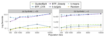
Figure 9: Running time of algorithms with respect to Population size.

5 Conclusions

In this paper, we introduced Guided Team-Partitioning, a new problem that repeatedly emerges in educational and organizational settings and cannot be addressed by existing team formation algorithms. From the computational viewpoint, we studied the computational complexity of the Guided Team-Partitioning problem and we proved that the problem is NP-hard to solve and approximate. We also proposed novel and efficient heuristic algorithms, which we evaluated via extensive experiments on both synthetic and real-world datasets. The results indicate our methodology is consistently able to deliver high-quality solutions and outperform multiple competitive baselines. Our work provides a platform for future research on problems

References

- [1] R. Agrawal, B. Golshan, and E. Terzi. Grouping students in educational settings. In SIGKDD, 2014.
- [2] A. Anagnostopoulos, L. Becchetti, C. Castillo, A. Gionis, and S. Leonardi. Online team formation in social networks. In WWW, 2012.
- [3] D. Arthur and S. Vassilvitskii. K-means++: The advantages of careful seeding. In SODA, 2007.
- [4] S. Bahargam, D. Erdos, A. Bestavros, and E. Terzi. Personalized education; solving a group formation and scheduling problem for educational content. In EDM, 2015.
- [5] S. Bahargam, D. Erdös, A. Bestavros, and E. Terzi. Team formation for scheduling educational material in massive online classes. CoRR, 2017.
- [6] S. Bahargam, B. Golshan, T. Lappas, and E. Terzi. A team-formation algorithm for faultline minimization. Expert Systems with Applications, 2019.
- [7] J. Bailey, M. Sass, P. M. Swiercz, C. Seal, and D. C. Kayes. Teaching with and through teams: Student-written, instructor-facilitated case writing and the signatory code. Journal of management education, 2005.
- [8] A. Bar-Hillel, T. Hertz, N. Shental, and D. Weinshall. Learning distance functions using equivalence relations. In ICML, 2003.
- [9] S. Basu, A. Banerjee, and R. Mooney. Semi-supervised clustering by seeding. In ICML, 2002.
- [10] S. G. Baugh and G. B. Graen. Effects of team gender and racial composition on perceptions of team performance in cross-functional teams. Group & Organization Management, 1997.
- [11] A. Baykasoglu, T. Dereli, and S. Das. Project team selection using fuzzy optimization approach. Cybern. Syst., 2007.
- [12] A. Bhowmik, V. S. Borkar, D. Garg, and M. Pallan. Submodularity in team formation problem. In SDM, 2014.
- [13] M. Bilenko and R. J. Mooney. Adaptive duplicate detection using learnable string similarity measures. In SIGKDD, 2003.
- [14] P. S. Bradley, K. P. Bennett, and A. Demiriz. Constrained k-means clustering. Technical report, Microsoft Research, 2000.
- [15] S. Chawla and A. Gionis. k-means-: A unified approach to clustering and outlier detection. In SDM, 2013.
- [16] D. Cohn, R. Caruana, and A. McCallum. Semi-supervised clustering with user feedback. Constrained Clustering: Advances in Algorithms, Theory, and Applications, 2003.
- [17] A. Demiriz, K. P. Bennett, and M. J. Embrechts. Semi-supervised clustering using genetic algorithms. Artificial neural networks in engineering, 1999.
- [18] J. Edmonds and R. M. Karp. Theoretical improvements in algorithmic efficiency for network flow problems. JACM, 1972.
- [19] B. Golshan, T. Lappas, and E. Terzi. Profit-maximizing cluster hires. In SIGKDD, 2014.
- [20] M. Hendriks, B. Voeten, and L. Kroep. Human resource allocation in a multi-project r&d environment: resource capacity allocation and project portfolio planning in practice. Journal of Project Management, 1999.
- [21] M. Kargar, M. Zihayat, and A. An. Finding affordable and collaborative teams from a network of experts. In SDM, 2013.
- [22] D. Klein, S. D. Kamvar, and C. D. Manning. From instance-level constraints to space-level constraints: Making the most of prior knowledge in data clustering. 2002.
- [23] T. Lappas, M. Crovella, and E. Terzi. Selecting a characteristic set of reviews. In SIGKDD, 2012.
- [24] T. Lappas, K. Liu, and E. Terzi. Finding a team of experts in social networks. In SIGKDD, 2009.
- [25] H. Pragarauskas and O. Gross. Multi-skill collaborative teams based on densest subgraphs. SDM, 2012.
- [26] S. S. Rangapuram, T. Bühler, and M. Hein. Towards realistic team formation in social networks based on densest subgraphs. In WWW, 2013.
- [27] N. Y. Razzouk, V. Seitz, and E. Rizkallah. Learning by doing: Using experiential projects in the undergraduate marketing strategy course. Marketing Education Review, 2003.
- [28] J. B. Shaw. A fair go for all? the impact of intragroup diversity and diversity-management skills on student experiences and outcomes in team-based class projects. Journal of Management Education, 2004.
- [29] D. B. Shmoys, E. Tardos, and K. Aardal. Approximation algorithms for facility location problems (extended abstract). In ACM Symposium on Theory of Computing, 1997.
- [30] I. M. Sobol’. On the distribution of points in a cube and the approximate evaluation of integrals. Zhurnal Vychislitel’noi Matematiki i Matematicheskoi Fiziki, 1967.
- [31] S. Tang. Profit-aware team grouping in social networks: A generalized cover decomposition approach. arXiv, 2016.
- [32] A. K. H. Tung, R. T. Ng, L. V. Lakshmanan, and J. Han. Constraint-based clustering in large databases, 2000.
- [33] K. Wagstaff, C. Cardie, S. Rogers, S. Schrödl, et al. Constrained k-means clustering with background knowledge. In ICML, 2001.
- [34] M. Walter and J. Zimmermann. Minimizing average project team size given multi-skilled workers with heterogeneous skill levels. Computers & Operations Research, 2016.
- [35] W. Wang, Z. He, P. Shi, W. Wu, and Y. Jiang. Truthful team formation for crowdsourcing in social networks. In AAMAS, 2016.
- [36] Y. Ye and E. Tse. An extension of karmarkar’s projective algorithm for convex quadratic programming. Mathematical Programming, 1989.