Classical quantum stochastic processes

Abstract

We investigate the role of coherence and Markovianity in finding an answer to the question whether the outcomes of a projectively measured quantum stochastic process are compatible with a classical stochastic process. For this purpose we put forward an operationally motivated definition of incoherent dynamics applicable to any open system’s dynamics. For non-degenerate observables described by rank-1 projective measurements we show that classicality always implies incoherent dynamics, whereas the converse is only true for invertible Markovian (but not necessarily time-homogeneous) dynamics. For degenerate observables the picture is somewhat reversed as classicality does no longer suffice to imply incoherent dynamics (even in the invertible Markovian case), while an incoherent, invertible Markovian dynamics still implies classicality.

I Introduction

Although in actual experiments with classical systems it might not always be possible to measure the system without disturbing it, at least theoretically one can consider the ideal limit of a non-invasive measurement. This idea has led to the theory of stochastic processes, a major mathematical toolbox used across many scientific disciplines van Kampen (2007); Gardiner (2009). Since the limit of an ideal non-disturbing measurement does not exist for quantum systems, a widely accepted consensus of what a quantum stochastic process actually is has not yet emerged. However, recent progress (see Ref. Milz et al. (2017) and references therein) strongly suggests that a quantum stochastic process is conceptually similar to classical causal modeling Pearl (2009) and here we will follow this approach. Understanding under which circumstances a projectively measured quantum system can be effectively described in a classical way is therefore of fundamental interest as it sheds light on the gap between quantum and classical stochastic processes. In addition, it enables us to distinguish quantum from classical features which is a relevant task for future technologies (e.g., in quantum information or quantum thermoydnamics) and for the field of quantum biology. Finally, it also has practical relevance as classical stochastic processes are easier to simulate.

The relation between classical and quantum stochastic processes was first addressed by Smirne and co-workers Smirne et al. (2018), who showed that the answer to the question whether a quantum system effectively behaves classical is closely related to the question whether coherences play a role in its evolution. More specifically, for a quantum dynamical semigroup obeying the regression theorem (i.e., a time-homogeneous quantum Markov process), it was shown that the statistics obtained from rank-1 projective measurements of a given system observable are compatible with a classical stochastic process if and only if the dynamics is “non-coherence-generating-and-detecting (NCGD)” Smirne et al. (2018).

The purpose of the present paper is to extend the results of Smirne et al. in various directions. We will provide an operationally motivated definition of incoherent dynamics, which is supposed to capture the absence of any detectable coherence in the dynamics. It is applicable to any open systems dynamics and it is different from the NCGD notion. Our definition allows us to prove the following: first, for non-degenerate observables described by rank-1 projectors, any process which can be effectively described classically is incoherent (i.e., cannot generate any detectable coherence), whereas the converse is only true for invertible Markovian, but not necessarily time-homogeneous dynamics. Second, for degenerate observables, we lose the property that classicality implies incoherent dynamics because detectable coherence can be hidden in degenerate subspaces.

The rest of the paper is structured as follows. In Sec. II we set the stage and introduce some basic definitions. Our main results are reported in Sec. III.1 for non-degenerate observables and in Sec. III.2 for degenerate observables. We conclude in Sec. IV. A thorough comparison with the framework of Ref. Smirne et al. (2018) is given in Appendix A showing that our results reduce to the ones of Smirne et al. in the respective limit. Various counterexamples, which demonstrate that our main theorems in Sec. III are tight, are postponed to Appendix B.

II Mathematical preliminaries

We start by reviewing basic notions of a classical stochastic process. We label the classical distinguishable states of the system of interest by $r$ and we assume that the system gets measured at an arbitrary set of discrete times $\{t_{1},\dots,t_{n}\}$. We denote the result at time $t_{i}$ by $r_{i}$. Furthermore, for reasons which will become clearer later on, we explicitly denote the initial preparation of the experiment by ${\cal{A}}_{0}$. At this stage the reader can think of this as merely a verbal description of how to initialize the experiment (e.g., ‘wait long enough such that the system is equilibrated and start measuring afterwards’), later on it will mathematically turn out to be a completely positive and trace-preserving map. We then denote the joint probability distribution to get the sequence of measurement results $\textbf{r}_{n}=r_{1},\dots,r_{n}$ at times $t_{1},\dots,t_{n}$ given the initial preparation ${\cal{A}}_{0}$ by

$$p(r_{n},t_{n};\dots;r_{1},t_{1}|{\cal{A}}_{0})\equiv p(\textbf{r}_{n}|{\cal{A}}_{0}).$$ (1)

The following definition is standard:

Definition II.1.

The probabilities $p(\textbf{r}_{n}|{\cal{A}}_{0})$ are said to be classical with repect to a given preparation procedure ${\cal{A}}_{0}$ if they fulfill the consistency condition

$$\sum_{r_{k}}p(r_{\ell},\dots,r_{k},\dots,r_{j}|{\cal{A}}_{0})=p(r_{\ell},\dots,\cancel{r_{k}},\dots,r_{j}|{\cal{A}}_{0})$$ (2)

for all $\ell\geq k\geq j\geq 1$. Here, the probability on the right hand side is constructed by measuring the states $r_{i}$ of the system only at the set of times $\{t_{\ell},\dots,t_{j}\}\setminus\{t_{k}\}$.

We remark that, if the consistency requirement (2) is fulfilled, then – by the Kolmogorov-Daniell extension theorem – we know that there exists an underlying continuous-in-time stochastic process, which contains all joint proabilities (1) as marginals. The importance of this theorem lies in the fact that it allows us to bridge experimental reality (where any measurement statistics is always finite) with its theoretical description (which often uses continuous-time dynamics in form of, e.g., stochastic differential equations).

Albeit condition (2) is in general not fulfilled for quantum dynamics, the joint probability distribution (1) is nevertheless a well-defined object in quantum mechanics. For this purpose we assume that the experimentalist measures at time $t_{k}$ an arbitrary system observable $R_{k}=\sum_{r_{k}}r_{k}P_{r_{k}}$ with projectors $P_{r_{k}}=P_{r_{k}}^{2}$ and eigenvalues $r_{k}\in\mathbb{R}$. If all projectors are rank-1, i.e., $P_{r_{k}}=|r_{k}{\rangle\langle}r_{k}|$, we talk about a non-degenerate system observable, otherwise we call it degenerate. Furthermore, following the conventional picture of open quantum systems Breuer and Petruccione (2002), we allow the system $S$ to be coupled to an arbitrary environment $E$. The initial system-environment state at time $t_{0}<t_{1}$ is denoted by $\rho_{SE}(t_{0})$. Then, by using superoperator notation, we can express Eq. (1) as

$$\begin{split}&p(\textbf{r}_{n}|{\cal{A}}_{0})\\ &=\mbox{tr}_{SE}\left\{{\cal{P}}_{r_{n}}{\cal{U}}_{n,n-1}\dots\cal{P}_{r_{2}}{\cal{U}}_{2,1}{\cal{P}}_{r_{1}}{\cal{U}}_{1,0}{\cal{A}}_{0}\rho_{SE}(t_{0})\right\}\\ &\equiv\mbox{tr}_{S}\left\{{\mathfrak{T}}_{n+1}[{\cal{P}}_{r_{n}},\dots,{\cal{P}}_{r_{2}},{\cal{P}}_{r_{1}},{\cal{A}}_{0}]\right\}.\end{split}$$ (3)

Here, the preparation procedure ${\cal{A}}_{0}$ is an arbitrary completely positive (CP) and trace-preserving map acting on the system only (we suppress identity operations in the tensor product notation). Notice that the preparation procedure could itself be the identity operation (i.e., ‘do nothing’) denoted by ${\cal{A}}_{0}={\cal{I}}_{0}$. Furthermore, ${\cal{U}}_{k,k-1}$ denotes the unitary time-evolution propagating the system-environment state from time $t_{k-1}$ to $t_{k}$ (we make no assumption about the underlying Hamiltonian here). We also introduced the projection superoperator ${\cal{P}}_{r_{k}}\rho\equiv P_{r_{k}}\rho P_{r_{k}}$, which acts only on the system and corresponds to result $r_{k}$ at time $t_{k}$. Finally, in the last line of Eq. (3) we have introduced the $(n+1)$-step ‘process tensor’ ${\mathfrak{T}}_{n+1}$ Pollock et al. (2018a) (also called ‘quantum comb’ Chiribella et al. (2008, 2009) or ‘process matrix’ Costa and Shrapnel (2016); Oreshkov and Giarmatzi (2016)). It is a formal but operationally well-defined object: it yields the (subnormalized) state of the system $\tilde{\rho}_{S}({\cal{P}}_{r_{n}},\dots,{\cal{P}}_{r_{2}},{\cal{P}}_{r_{1}},{\cal{A}}_{0})={\mathfrak{T}}_{n+1}[{\cal{P}}_{r_{n}},\dots,{\cal{P}}_{r_{2}},{\cal{P}}_{r_{1}},{\cal{A}}_{0}]$ conditioned on a certain sequence of interventions ${\cal{P}}_{r_{n}},\dots,{\cal{P}}_{r_{2}},{\cal{P}}_{r_{1}},{\cal{A}}_{0}$. Its norm, as given by the trace over $S$, equals the probability to obtain the measurement results $\textbf{r}_{n}$. Recently, it was shown that the process tensor allows for a rigorous definition of quantum stochastic processes (or quantum causal models) fulfilling a generalized version of the Kolmogorov-Daniell extension theorem Milz et al. (2017). We also add that complete knowledge of the process tensor ${\mathfrak{T}}_{n}$ implies complete knowledge of the process tensor ${\mathfrak{T}}_{\ell}$ for $\ell\leq n$, i.e., ${\mathfrak{T}}_{n}$ contains ${\mathfrak{T}}_{\ell}$.

We now have the main tools at hand to precisely state the question we are posing in this paper: Which conditions does a quantum stochastic process need to fulfill in order to guarantee that the resulting measurement statistics can (or cannot) be explained by a classical stochastic process? That is, when is Eq. (2) fulfilled or, in terms of the process tensor, when is

$$\begin{split}&\mbox{tr}_{S}\{{\mathfrak{T}}_{\ell+1}[{\cal{P}}_{r_{\ell}},\dots,\Delta_{k},\dots,{\cal{P}}_{r_{j}},\dots,{\cal{A}}_{0}]\}\\ &\stackrel{{\scriptstyle?}}{{=}}\mbox{tr}_{S}\{{\mathfrak{T}}_{\ell+1}[{\cal{P}}_{r_{\ell}},\dots,{\cal{I}}_{k},\dots,{\cal{P}}_{r_{j}},\dots,{\cal{A}}_{0}]\}.\end{split}$$ (4)

Here, we have introduced the dephasing operation at time $t_{k}$, $\Delta_{k}\equiv\sum_{r_{k}}{\cal{P}}_{r_{k}}$, which plays an essential role in the following. Furthermore, the dots in Eq. (LABEL:eq_classicality_process_tensor) denote either projective measurements (if the system gets measured at that time) or identity operations (if the system does not get measured at that time).

To answer the question, we will need a suitable notion of an ‘incoherent’ quantum stochastic process, defined as follows:

Definition II.2.

For a given set of observables $\{R_{k}\}$, $k\in\{1,\dots,\ell\}$, we call the dynamics of an open quantum system $\ell$-incoherent with respect to the preparation ${\cal{A}}_{0}$ if all process tensors

$${\mathfrak{T}}_{\ell+1}\left[\Delta_{\ell},\left\{\begin{matrix}\Delta_{\ell-1}\\ {\cal{I}}_{\ell-1}\\ \end{matrix}\right\},\dots,\left\{\begin{matrix}\Delta_{1}\\ {\cal{I}}_{1}\\ \end{matrix}\right\},{\cal{A}}_{0}\right]$$ (5)

are equal. Here, the angular bracket notation means that at each time step we can freely choose to perform either a dephasing operation ($\Delta$) or nothing (${\cal{I}}$). If the dynamics are $\ell$-incoherent for all $\ell\in\{1,\dots,n\}$, we simply call the dynamics incoherent with respect to the preparation procedure ${\cal{A}}_{0}$.

This definition is supposed to capture the situation where the experimentalist has no ability to detect the presence of coherence during the course of the evolution. For this purpose we imagine that the experimentalist can manipulate the system in two ways: first, she can prepare the initial system state in some way via ${\cal{A}}_{0}$ (which could be only the identity operation) and she can projectively measure the system observables $R_{k}$ at times $t_{k}\in\{t_{1},\dots,t_{n}\}$. The question is then: if the final state got dephased with respect to the observable $R_{\ell}$ (e.g., by performing a final measurement of $R_{\ell}$), is the experimentalist able to infer whether the system was subjected to additional dephasing operations at earlier times, i.e., can possible coherences at earlier times become manifest in different populations at the final time $t_{\ell}$? If that is not the case, the dynamics are called $\ell$-incoherent. We remark that a process that is $\ell$-incoherent is not necessarily $k$-incoherent for $k\neq\ell$. It is therefore important to specify at which (sub)set of times the process is incoherent. In the following we will be only interested in processes which are $\ell$-incoherent for all $\ell\in\{1,\dots,n\}$, henceforth dubbed simply ‘incoherent’ (with respect to the preparation ${\cal{A}}_{0}$). We repeat that our definition of incoherence is different from the NCGD notion introduced in Ref. Smirne et al. (2018), see Appendix A. Furthermore, a similar idea restricted to two times was introduced in Ref. Gessner and Breuer (2011) in order to detect nonclassical system-environment correlations in the dynamics of open quantum systems.

III Results

III.1 Non-degenerate observables

Our first main result is the following:

Theorem III.1.

If the measurement statistics are classical with respect to ${\cal{A}}_{0}$, then the dynamics is incoherent with respect to ${\cal{A}}_{0}$.

Before we prove it, we remark that this theorem holds for any quantum stochastic process (especially without imposing Markovianity). Furthermore, a classical process for the times $\{t_{n},\dots,t_{1}\}$ is also classical for all subsets of times and hence, the theorem implies incoherence, i.e., $\ell$-incoherence for all $\ell\in\{1,\dots,n\}$. In the following proof we will only display the case $\ell=n$, as the rest follows immediately.

Proof.

We start by noting that

$${\mathfrak{T}}_{n+1}[{\cal{P}}_{r_{n}},\dots,{\cal{P}}_{r_{1}},{\cal{A}}_{0}]=p(r_{n},\dots,r_{1}|{\cal{A}}_{0})|r_{n}{\rangle\langle}r_{n}|,$$ (6)

which is a general identity as we have not made any assumption about the joint probability $p(r_{n},\dots,r_{1}|{\cal{A}}_{0})$. Obviously, if we choose to perform nothing at any time $t_{\ell}<t_{n}$, we have

$$\begin{split}&{\mathfrak{T}}_{n+1}[{\cal{P}}_{r_{n}},\dots,{\cal{I}}_{\ell},\dots,{\cal{P}}_{r_{1}},{\cal{A}}_{0}]\\ &=p(r_{n},\dots,\cancel{r_{\ell}},\dots,r_{1}|{\cal{A}}_{0})|r_{n}{\rangle\langle}r_{n}|.\end{split}$$ (7)

But by assumption of classicality, this is equal to

$$\begin{split}&{\mathfrak{T}}_{n+1}[{\cal{P}}_{r_{n}},\dots,{\cal{I}}_{\ell},\dots,{\cal{P}}_{r_{1}},{\cal{A}}_{0}]\\ &=\sum_{r_{\ell}}p(r_{n},\dots,r_{\ell},\dots,r_{1}|{\cal{A}}_{0})|r_{n}{\rangle\langle}r_{n}|\\ &=\sum_{r_{\ell}}{\mathfrak{T}}_{n+1}[{\cal{P}}_{r_{n}},\dots,{\cal{P}}_{r_{\ell}},\dots,{\cal{P}}_{r_{1}},{\cal{A}}_{0}]\\ &={\mathfrak{T}}_{n+1}[{\cal{P}}_{r_{n}},\dots,\Delta_{\ell},\dots,{\cal{P}}_{r_{1}},{\cal{A}}_{0}].\end{split}$$ (8)

Hence, by summing Eq. (8) over the remaining $r_{k}\neq r_{\ell}$, we confirm

$$\begin{split}&{\mathfrak{T}}_{n+1}[\Delta_{n},\dots,{\cal{I}}_{\ell},\dots,\Delta_{1},{\cal{A}}_{0}]\\ &={\mathfrak{T}}_{n+1}[\Delta_{n},\dots,\Delta_{\ell},\dots,\Delta_{1},{\cal{A}}_{0}]\end{split}$$ (9)

for arbitrary $t_{\ell}<t_{n}$ and where the dots denote dephasing operations at the remaining times. We can now pick another arbitrary time $t_{k}\neq t_{\ell}$ and repeat essentially the same steps as above to arrive at the conclusion

$$\begin{split}&{\mathfrak{T}}_{n+1}[\Delta_{n},\dots,{\cal{I}}_{\ell},\dots,{\cal{I}}_{k},\dots,\Delta_{1},{\cal{A}}_{0}]\\ &={\mathfrak{T}}_{n+1}[\Delta_{n},\dots,\Delta_{\ell},\dots,\Delta_{k},\dots,\Delta_{1},{\cal{A}}_{0}]\end{split}$$ (10)

for any two times $t_{k}\neq t_{\ell}$. By repeating this argument further, we finally confirm that the dynamics are incoherent. ∎

The converse of Theorem III.1 holds only in a stricter sense. For this purpose we need the notion of Markovianity as defined in Ref. Pollock et al. (2018b). In there, it was shown that the definition of a quantum Markov process implies the notion of operational CP divisibility. This means that for an arbitrary set of independent interventions (CP maps) ${\cal{A}}_{r_{n}},\dots,{\cal{A}}_{r_{0}}$ the process tensor ‘factorizes’ as

$${\mathfrak{T}}_{n+1}[{\cal{A}}_{r_{n}},\dots,{\cal{A}}_{r_{0}}]={\cal{A}}_{r_{n}}\Lambda_{n,n-1}\dots\Lambda_{1,0}{\cal{A}}_{r_{0}}\rho_{S}(t_{0}).$$ (11)

Here, the set $\{\Lambda_{\ell,k}\}$ is a family of CP and trace-preserving maps fulfilling the composition law $\Lambda_{\ell,j}=\Lambda_{\ell,k}\Lambda_{k,j}$ for any $\ell>k>j$. We remark that a CP divisible process (which is commonly refered to as being ‘Markovian’) is in general not operationally CP divisible (also see the recent discussion in Ref. Milz et al. (2019a)). In a nutshell, an operationally CP divisible process always fulfills the quantum regression theorem, but a CP divisible process does not (a counterexample is in fact shown in Appendix A).

Furthermore, to establish the converse of Theorem III.1 we also need the following definition:

Definition III.1.

A Markov process $\{\Lambda_{\ell,k}\}$ is said to be invertible, if the inverse of any $\Lambda_{k,0}$ exists for all $k$, i.e., the CP and trace-preserving maps $\Lambda_{\ell,k}$ are identical to $\Lambda_{\ell,0}\Lambda_{k,0}^{-1}$.

We are now ready to prove the next main theorem:

Theorem III.2.

If the dynamics are Markovian, invertible and incoherent for all preparations ${\cal{A}}_{0}$, then the statistics are classical for any preparation.

Proof.

By using Eq. (11) and the property of incoherence, we can conclude that for any two times $t_{\ell+1},t_{\ell}\in\{t_{1},\dots,t_{n}\}$ (with $t_{\ell+1}>t_{\ell}$)

$$\Delta_{\ell+1}\Lambda_{\ell+1,\ell}\Delta_{\ell}\Lambda_{\ell,0}{\cal{A}}_{0}\rho_{S}(t_{0})=\Delta_{\ell+1}\Lambda_{\ell+1,\ell}\Lambda_{\ell,0}{\cal{A}}_{0}\rho_{S}(t_{0}).$$ (12)

Since the dynamics are invertible and incoherent for all preparations ${\cal{A}}_{0}$, this implies the superoperator identity $\Delta_{\ell+1}\Lambda_{\ell+1,\ell}\Delta_{\ell}=\Delta_{\ell+1}\Lambda_{\ell+1,\ell}$. By multiplying this equation with ${\cal{P}}_{r_{\ell+1}}$, we arrive at

$$\sum_{r_{\ell}}{\cal{P}}_{r_{\ell+1}}\Lambda_{\ell+1,\ell}{\cal{P}}_{r_{\ell}}={\cal{P}}_{r_{\ell+1}}\Lambda_{\ell+1,\ell}.$$ (13)

From this general identity we immediately obtain that

$$\begin{split}&\sum_{r_{\ell}}p(\textbf{r}_{n})\\ &=\mbox{tr}\left\{{\cal{P}}_{r_{n}}\Lambda_{n,n-1}\dots\sum_{r_{\ell}}{\cal{P}}_{r_{\ell+1}}\Lambda_{\ell+1,\ell}{\cal{P}}_{r_{\ell}}\dots\cal{P}_{r_{1}}\Lambda_{1,0}{\cal{A}}_{0}\rho\right\}\\ &=\mbox{tr}\{{\cal{P}}_{r_{n}}\Lambda_{n,n-1}\dots\cal{P}_{r_{\ell+1}}\Lambda_{\ell+1,\ell}\dots\cal{P}_{r_{1}}\Lambda_{1,0}{\cal{A}}_{0}\rho\}\\ &=p(r_{n},\dots,\cancel{r_{\ell}},\dots,r_{1}).\end{split}$$ (14)

This concludes the proof as the above argument also holds for all possible subsets of times. ∎

We add that the counterexamples in Appendix B demonstrate that Theorem III.2 is also tight in the sense that a process, which is incoherent only for a subset of preparations or which is not invertible, does not imply classical statistics. One remaining open question concerns the assumption of Markovianity. At the moment it is not clear whether relaxing this condition is meaningful as it requires to define the notion of invertibility for a non-Markovian process, which is not unambiguous.

Furthermore, the superoperator identity (13) implies that, if we write $\Lambda_{\ell,k}$ as a matrix in an ordered basis where populations precede coherences with respect to the measured observable $R_{k}$ (input) and $R_{\ell}$ (output), it has the form

$$\Lambda_{\ell,k}=\begin{pmatrix}A_{\ell,k}&0\\ C_{\ell,k}&D_{\ell,k}\\ \end{pmatrix},$$ (15)

where $A_{\ell,k}$ is a stochastic matrix and $C_{\ell,k}$ and $D_{\ell,k}$ are matrices, which are only constrained by the requirement of complete positivity.

III.2 Degenerate observables

If the measured observable contains degeneracies, the picture above somewhat reverses. First, Theorem III.1 ceases to hold even in the Markovian and invertible regime because the assumption of a non-degenerate observable already entered in the first step of its proof, see Eq. (6). Physically speaking, the reason is that it now becomes possible to hide coherences in degenerate subspaces and this can have a detectable effect on the output state (5). This is demonstrated with the help of an example in Appendix B. In contrast, Theorem III.2 still holds true for degenerate observables. In fact, in the proof of Theorem III.2 we never used that the measured observable is non-degenerate.

IV Conclusions

We have investigated whether the outcomes of a projectively measured quantum system can be described classically depending on the capability of an open quantum system to show detectable effects of coherence. The question whether the quantum stochastic process is (invertible) Markovian and whether the measured observables are degenerate (or not) had a crucial influence on the results. Together with the counterexamples in Appendix B we believe that we have provided a fairly complete picture about the interplay between classicality, coherence and Markovianity. It remains, however, still open whether our definition of ‘incoherent dynamics’ is the most meaningful one. One clear advantage of our proposal is that it is operationally and theoretically well-defined for arbitrary quantum processes. Therefore, it could help to extend existing resource theories, which crucially rely on the existence of dynamical maps Streltsov et al. (2017), to arbitrary multi-time processes.

We further point out that our investigation is closely related to the study of Leggett-Garg inequalities and possible violations thereof Leggett and Garg (1985); Emary et al. (2014). In fact, the classicality assumption (2) plays a crucial role in deriving any Leggett-Garg inequality. Therefore, we can conclude that all incoherent quantum systems, which evolve in an invertible Markovian way, will never violate a Leggett-Garg inequality if the measured observable is non-degenerate. Interestingly, incoherent quantum systems could potentially violate Leggett-Garg inequalities if the measured observable is degenerate.

Another interesting open point of investigation concerns the question whether the property of incoherence implies a particular structure on the generator of a quantum master equation, which is still the primarily used tool in open quantum system theory. This question is indeed further pursued by one of us et al. .

Note added. While this manuscript was under review, we became aware of the work of Milz et al. Milz et al. (2019b) where an identical question is analysed from a related perspective.

Acknowledgments

PS is financially supported by the DFG (project STR 1505/2-1) and MGD by ‘la Caixa’ Foundation, grant LCF/BQ/DE16/11570017. We also acknowledge funding from the Spanish MINECO FIS2016-80681-P (AEI-FEDER, UE).

Appendix A Comparison with the framework of Smirne et al.

In Ref. Smirne et al. (2018) the notion of “non-coherence-generating-and-detecting dynamics” (NCGD dynamics) was introduced based on the following definition:

Definition A.1.

The dynamics of an open quantum system is called NCGD with respect to the set of observables $\{R_{k}\}$ if

$$\Delta_{\ell}\Lambda_{\ell,k}\Delta_{k}\Lambda_{k,j}\Delta_{j}=\Delta_{\ell}\Lambda_{\ell,j}\Delta_{j}$$ (16)

for all $t_{\ell}\geq t_{k}\geq t_{j}\geq t_{1}$.

In this definition $\Lambda_{\ell,k}$ denotes the ‘dynamical map’ of the quantum system from time $t_{k}$ to time $t_{\ell}$. For instance, for a time-dependent master equation with Liouvillian ${\cal{L}}(t)$ this is defined as

$$\Lambda_{\ell,k}={\cal{T}}_{+}\exp\left[\int_{t_{k}}^{t_{\ell}}{\cal{L}}(t)dt\right],$$ (17)

where ${\cal{T}}_{+}$ denotes the time-ordering operator.

To compare the notions of NCGD and incoherent dynamics, we start by noting that both are almost identical if the dynamics are Markovian, invertible and subjected to measurements of a non-degenerate system observable. This is important as we are thereby able to confirm the results of Ref. Smirne et al. (2018) in an independent way. To see this, we first prove the following statement:

Theorem A.1.

If the dynamics are Markovian, invertible and incoherent for all possible preparations, then they are also NCGD.

Proof.

By assumption of incoherence we have for an arbitrary preparation ${\cal{A}}_{0}$ and an arbitrary set of times $\{t_{\ell},t_{k},t_{j}\}$ with $\ell\geq k\geq j\geq 1$

$$\begin{split}&{\mathfrak{T}}_{\ell+1}[\Delta_{\ell},\dots,\Delta_{k},\dots,\Delta_{j},\dots,{\cal{A}}_{0}]\\ &={\mathfrak{T}}_{\ell+1}[\Delta_{\ell},\dots,{\cal{I}}_{k},\dots,\Delta_{j},\dots,{\cal{A}}_{0}],\end{split}$$ (18)

where the dots denote identity operations. By Markovianity, this means that

$$\Delta_{\ell}\Lambda_{\ell,k}\Delta_{k}\Lambda_{k,j}\Delta_{j}\Lambda_{j,0}{\cal{A}}_{0}\rho_{0}=\Delta_{\ell}\Lambda_{\ell,j}\Delta_{j}\Lambda_{j,0}{\cal{A}}_{0}\rho_{0}.$$ (19)

Since ${\cal{A}}_{0}$ is arbitrary and the dynamics are assumed to be invertible, this implies

$$\Delta_{\ell}\Lambda_{\ell,k}\Delta_{k}\Lambda_{k,j}\Delta_{j}=\Delta_{\ell}\Lambda_{\ell,j}\Delta_{j}.$$ (20)

Hence, the dynamics are NCGD. ∎

The ‘converse’ of Theorem A.1 reads as follows

Theorem A.2.

If the dynamics is Markovian and NCGD, the dynamics is incoherent with respect to all preparations that result in a diagonal state (with respect to the observable $R_{1}$) at time $t_{1}$.

Proof.

Since the dynamics is Markovian and the state at time $t_{1}$ is diagonal, we always have

$$\begin{split}&{\mathfrak{T}}_{n+1}\left[\Delta_{n},\left\{\begin{matrix}\Delta_{n-1}\\ {\cal{I}}_{n-1}\\ \end{matrix}\right\},\dots,\left\{\begin{matrix}\Delta_{1}\\ {\cal{I}}_{1}\\ \end{matrix}\right\},{\cal{A}}_{0}\right]\\ &={\mathfrak{T}}_{n+1}\left[\Delta_{n},\left\{\begin{matrix}\Delta_{n-1}\\ {\cal{I}}_{n-1}\\ \end{matrix}\right\},\dots,\Delta_{1},{\cal{A}}_{0}\right].\end{split}$$ (21)

Hence, the dynamics are ‘sandwiched’ by two dephasing operations at the beginning at time $t_{1}$ and at the end at time $t_{n}$. By the property of NCGD, we are allowed to introduce arbitrary dephasing/identity operations at any time step $t_{k}$, $n>k>1$. Hence, the dynamics are incoherent. ∎

This proves that our main results are not in contradiction to Ref. Smirne et al. (2018): In there it was shown that a Markovian time-homogeneous process – a subclass of invertible Markov processes, which are described by a time-independent Liouvillian ${\cal{L}}$ – is classical with respect to measurements of a non-degenerate observable for an initially diagonal state if and only if the dynamics are NCGD.

Without the three assumptions of invertibility, Markovianity and non-degeneracy of the measured observable, notable differences start to appear. First, our definition of incoherent dynamics remains meaningful even if the dynamics are not invertible or if the measured observable is degenerate: in the first case, the dynamical map $\Lambda_{\ell,k}$ is not unambiguously defined for $t_{k}>t_{0}$ and in the second case, even $\Lambda_{k,0}$ might not be defined if the system remains entangled with the environment after an initial dephasing operation. Most notably, however, in the non-Markovian regime Eq. (16) cannot directly be checked in an experiment by comparing two sets of ensembles, one which was dephased in the middle of the evolution and one which was not. Indeed, if the dynamics are non-Markovian, then the dynamics after a dephasing operation at time $t_{k}$ will not be described by the map $\Lambda_{\ell,k}=\Lambda_{\ell,0}\Lambda_{k,0}^{-1}$. We will exemplify this point by an example, which was also considered in Refs. Pollock et al. (2018b); Smirne et al. (2018) and experimentally realized in Ref. Liu et al. (2011).

The model describes a spin coupled to a continuous degree of freedom via the Hamiltonian $H_{SE}=\frac{g}{2}\sigma_{z}\otimes\hat{q}$. The initial state of the environment is taken to be pure with a wavefunction in coordinate representation $\psi_{E}(q)=\sqrt{\gamma/\pi}/(q+i\gamma)$. For an initially decorrelated system-environment state the exact reduced system dynamics are $\rho(t)=\mbox{tr}_{E}\{e^{-iH_{SE}t}\rho(0)\otimes|\psi\rangle_{E}\langle\psi|e^{-iH_{SE}t}\}$. Evaluating the trace in the coordinate basis and using $e^{i\alpha\sigma_{z}}=\cos\alpha+i\sin\alpha\sigma_{z}$, it is easy to confirm that

$$\begin{split}\rho(t)=\int dq&\frac{\gamma/\pi}{q^{2}+\gamma^{2}}\left[\cos\left(\frac{gq}{2}t\right)-i\sin\left(\frac{gq}{2}t\right)\sigma_{z}\right]\\ &\times\rho(0)\left[\cos\left(\frac{gq}{2}t\right)+i\sin\left(\frac{gq}{2}t\right)\sigma_{z}\right].\end{split}$$ (22)

Explicit evaluation of the integrals yields

$$\rho(t)=\frac{1}{2}(1+e^{-\Gamma t})\rho(0)+\frac{1}{2}(1-e^{-\Gamma t})\sigma_{z}\rho(0)\sigma_{z},$$ (23)

where we have introduced the dephasing rate $\Gamma\equiv g\gamma$. Next, we take Eq. (23), substract $\sigma_{z}$(23)$\sigma_{z}$ and multiply by $e^{-\Gamma t}/2$ to confirm that

$$\frac{e^{-\Gamma t}}{2}[\rho(0)-\sigma_{z}\rho(0)\sigma_{z}]=\frac{1}{2}\rho(t)-\frac{1}{2}\sigma_{z}\rho(t)\sigma_{z}.$$ (24)

This allows us to deduce a master equation for the two-level system by taking the time-derivative of Eq. (23) and by using the previous result:

$$\begin{split}\partial_{t}\rho(t)&=-\Gamma\frac{e^{-\Gamma t}}{2}[\rho(0)-\sigma_{z}\rho(0)\sigma_{z}]\\ &=\frac{\Gamma}{2}[\sigma_{z}\rho(t)\sigma_{z}-\rho(t)]\\ &=\frac{\Gamma}{2}\left[\sigma_{z}\rho(t)\sigma_{z}-\frac{1}{2}\{\sigma_{z}^{2},\rho(t)\}\right]=\equiv{\cal{L}}\rho(t),\end{split}$$ (25)

where ${\cal{L}}$ denotes the ‘Liouvillian’. This is a very simple master equation where the expectation values of the Pauli matrices $[x(t),y(t),z(t)]=[{\left\langle{\sigma_{x}}\right\rangle}(t),{\left\langle{\sigma_{y}}\right\rangle}(t),{\left\langle{\sigma_{z}}\right\rangle}(t)]$ obey the differential equations

$$\dot{x}(t)=-\Gamma x(t),~{}~{}\dot{y}(t)=-\Gamma y(t),~{}~{}\dot{z}(t)=0.$$ (26)

The solution of these equations is obvious.

Next, let us apply a dephasing operation in the $\sigma_{x}$ basis at an arbitrary time $s>0$, which is defined for any $\rho$ as

$$\Delta\rho=|+{\rangle\langle}+|\rho|+{\rangle\langle}+|+|-{\rangle\langle}-|\rho|-{\rangle\langle}-|,$$ (27)

where $|\pm\rangle=(|1\rangle\pm|0\rangle)/\sqrt{2}$. Note that for a density matrix parametrized by a Bloch vector $(x,y,z)$ in the $\sigma_{z}$ basis we obtain

$$\Delta\frac{1}{2}\begin{pmatrix}1+z&x-iy\\ x+iy&1-z\\ \end{pmatrix}=\frac{1}{2}\begin{pmatrix}1&x\\ x&1\\ \end{pmatrix}.$$ (28)

We now want to compute the exact system state at time $t>s$ after a dephasing operation was applied, i.e.,

$$\rho(t)=\mbox{tr}\{{\cal{U}}_{t,t-s}\Delta{\cal{U}}_{s,0}\rho(0)\otimes|\psi\rangle_{E}\langle\psi|\}.$$ (29)

By evaluating the trace again in the coordinate representation, this can be done straightforwardly although the calculation becomes now more tedious. The result for an initial state with expectation value ${\left\langle{\sigma_{x}}\right\rangle}(0)=x_{0}$ [the other expectation values do not matter as they get erased in the dephasing operation, cf. Eq. (28)] is

$$\begin{split}x(t)=&~{}\frac{x_{0}}{2}\left\{\cosh[\Gamma(t-2s)]+\cosh(\Gamma t)\right\}\\ &-\frac{x_{0}}{2}\left\{\sinh(\Gamma t)+\frac{\sinh[\Gamma(t-2s)]}{\text{sign}(t-2s)}\right\}.\end{split}$$ (30)

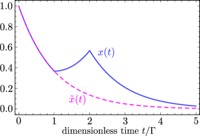
Figure 1: Plot of the exact time evolution [Eq. (30), solid blue line] compared with the approximated one [Eq. (32), dashed pink line]. Parameters are $\Gamma=1,s=1$ and $x_{0}=1$.

Now, for time-homogeneous dynamics the definition of NCGD in Ref. Smirne et al. (2018) reduces to

$$\Delta e^{{\cal{L}}(t-s)}\Delta e^{{\cal{L}}s}\Delta=\Delta e^{{\cal{L}}t}\Delta$$ (31)

for all $t>s>0$. For our example we get according to the dynamics in Eq. (31)

$$\tilde{x}(t)=\mbox{tr}\{\sigma_{x}e^{{\cal{L}}(t-s)}\Delta e^{{\cal{L}}s}\Delta\rho(0)\}=e^{-\Gamma t}x_{0}$$ (32)

for all $t$ and especially independent of any dephasing operation. Hence, the dynamics is NCGD according to the definition from Ref. Smirne et al. (2018). But by looking at the exact time-evolution of the system [cf. Eq. (30) and Fig. 1], we see that even the mean value $x(t)$ can show a strong dependence on the dephasing operation. Therefore, according to our definition, the dynamics are not incoherent with respect to the $\sigma_{x}$ basis.

Finally, we mention that there are a couple of finer details too. For instance, in our work we only consider a fixed set of discrete times whereas Smirne et al. allow for arbitrary times. On the other hand, the system observable $R_{k}$ was not allowed to be explicitly time-dependent in Ref. Smirne et al. (2018). These points can be, however, incorporated in each of the frameworks and therefore we did not put any additional emphasis on these minor details.

Appendix B Counterexamples

A process which is incoherent for one preparation ${\cal{A}}_{0}$ but not classical for that preparation

Consider an isolated two-level system undergoing purely unitary dynamics. Then, the dynamics are incoherent with respect to any preparation ${\cal{A}}_{0}$ which maps the system state to a completely mixed state: independent of any dephasing or identity operation, the state will stay at the origin of the Bloch ball for all times.

However, such a dynamics does not necessarily imply classical statistics. Consider, e.g., the measurement basis to be $\sigma_{z}$ (with outcomes $\{\uparrow_{k},\downarrow_{k}\}$ at times $t_{k}$) and the unitary rotations to be around the $y$-axis. Furthermore, the time-steps are chosen equidistant in such a way that the rotation is exactly $\pi/2$. It is then easy to confirm that

$$p(\uparrow_{3},\uparrow_{2},\uparrow_{1})=p(\uparrow_{3},\downarrow_{2},\uparrow_{1})=\frac{1}{8},$$ (33)

hence, $\sum_{\sigma_{2}\in\{\uparrow,\downarrow\}}p(\uparrow_{3},\sigma_{2},\uparrow_{1})=1/4$. But if we do not perform any measurement at time $t_{2}$, we obtain ${p(\uparrow_{3},\cancel{\sigma_{2}},\uparrow_{1})=0}$. The statistics are therefore non-classical.

A process which is Markovian and incoherent for all preparations but not classical

Consider a Markov process for a two-level system where the map in the first time-step is defined by

$$\Lambda_{2,1}:\rho\mapsto\frac{1}{2}\begin{pmatrix}1&0\\ 0&1\\ \end{pmatrix}$$ (34)

for any input state $\rho$. The rest of the dynamics is again unitary as in the previous counterexample. Thus, the dynamics are incoherent for any preparation, but not classical.

A process which is Markovian, invertible and classical for all preparations but not incoherent with respect to measurements of a degenerate observable

Consider two qubits $A$ and $B$ and projective measurements in some fixed basis of qubit $A$ only such that the dephasing operation acts only locally on qubit $A$: $\Delta=\Delta_{A}\otimes{\cal{I}}_{B}$. Thus, the measured observable is degenerate and projects onto two possible subspaces of dimension two. Furthermore, we only consider measurements at two times $t_{2}$ and $t_{1}$ and assume the dynamics in between these two times to be described by a unitary swap gate, $U_{\text{swap}}|i_{A}j_{B}\rangle=|j_{B}i_{A}\rangle$. We also assume that the dynamics in between the preparation and the first measurement is trivial, i.e., described by an identity operation.

Now, consider an arbitrary initial state resulting from an arbitrary preparation ${\cal{A}}_{0}$, denoted as

$${\cal{A}}_{0}\rho_{0}=\sum_{i_{A},i_{B},j_{A},j_{B}}\rho_{i_{A}i_{B},j_{A}j_{B}}|i_{A}i_{B}{\rangle\langle}j_{A}j_{B}|.$$ (35)

Then, straightforward calculation reveals that

$$p(r_{2},r_{1}) =\mbox{tr}_{AB}\{{\cal{P}}_{r_{2}}{\cal{U}}_{\text{swap}}{\cal{P}}_{r_{1}}{\cal{A}}_{0}\rho_{0}\}=\rho_{r_{1}r_{2},r_{1}r_{2}},$$ (36)

$$p(r_{2},\cancel{r_{1}}) =\mbox{tr}_{AB}\{{\cal{P}}_{r_{2}}{\cal{U}}_{\text{swap}}{\cal{A}}_{0}\rho_{0}\}=\sum_{j}\rho_{jr_{2},jr_{2}}.$$ (37)

Hence, the process is classical: $\sum_{r_{1}}p(r_{2},r_{1})=p(r_{2},\cancel{r_{1}})$.

However, the process is not incoherent. Consider, for instance, the initial state

$${\cal{A}}_{0}\rho_{0}=|\psi_{0}{\rangle\langle}\psi_{0}|,~{}~{}~{}|\psi_{0}\rangle=\frac{|0_{A}\rangle+|1_{A}\rangle}{\sqrt{2}}\otimes|0_{B}\rangle.$$ (38)

Then,

$${\mathfrak{T}}_{3}[\Delta_{2},{\cal{I}}_{1},{\cal{A}}_{0}]=|\psi_{1}{\rangle\langle}\psi_{1}|,~{}~{}~{}|\psi_{1}\rangle=|0_{A}\rangle\otimes\frac{|0_{B}\rangle+|1_{B}\rangle}{\sqrt{2}},$$ (39)

but

$${\mathfrak{T}}_{3}[\Delta_{2},\Delta_{1},{\cal{A}}_{0}]=\frac{|0_{A}0_{B}{\rangle\langle}0_{A}0_{B}|+|0_{A}1_{B}{\rangle\langle}0_{A}1_{B}|}{2}.$$ (40)

References

- van Kampen (2007) N. G. van Kampen, Stochastic Processes in Physics and Chemistry (North-Holland Publishing Company, Amsterdam, 3rd ed., 2007).
- Gardiner (2009) C. Gardiner, Stochastic Methods: A Handbook for the Natural and Social Sciences (Springer-Verlag, Berlin Heidelberg, 2009).
- Milz et al. (2017) S. Milz, F. Sakuldee, F. A. Pollock, and K. Modi, “Kolmogorov extension theorem for (quantum) causal modelling and general probabilistic theories,” arXiv: 1712.02589 (2017).
- Pearl (2009) J. Pearl, Causality: Models, Reasoning and Inference (Cambridge University Press, 2009).
- Smirne et al. (2018) A. Smirne, D. Egloff, M. G. Díaz, M. B. Plenio, and S. F. Hulega, “Coherence and non-classicality of quantum Markov processes,” Quantum Sci. Technol. 4, 01LT01 (2018).
- Breuer and Petruccione (2002) H.-P. Breuer and F. Petruccione, The Theory of Open Quantum Systems (Oxford University Press, Oxford, 2002).
- Pollock et al. (2018a) F. A. Pollock, C. Rodríguez-Rosario, T. Frauenheim, M. Paternostro, and K. Modi, “Non-Markovian quantum processes: Complete framework and efficient characterization,” Phys. Rev. A 97, 012127 (2018a).
- Chiribella et al. (2008) G. Chiribella, G. M. D’Ariano, and P. Perinotti, “Quantum circuit architecture,” Phys. Rev. Lett. 101, 060401 (2008).
- Chiribella et al. (2009) G. Chiribella, G. M. D’Ariano, and P. Perinotti, “Theoretical framework for quantum networks,” Phys. Rev. A 80, 022339 (2009).
- Costa and Shrapnel (2016) F. Costa and S. Shrapnel, “Quantum causal modelling,” New J. Phys. 18, 063032 (2016).
- Oreshkov and Giarmatzi (2016) O. Oreshkov and C. Giarmatzi, “Causal and causally separable processes,” New J. Phys. 18, 093020 (2016).
- Gessner and Breuer (2011) M. Gessner and H.-P. Breuer, “Detecting nonclassical system-environment correlations by local operations,” Phys. Rev. Lett. 107, 180402 (2011).
- Pollock et al. (2018b) F. A. Pollock, C. Rodríguez-Rosario, T. Frauenheim, M. Paternostro, and K. Modi, “Operational Markov condition for quantum processes,” Phys. Rev. Lett. 120, 040405 (2018b).
- Milz et al. (2019a) S. Milz, M. S. Kim, F. A. Pollock, and K. Modi, “CP divisibility does not mean Markovianity,” arXiv: 1901.05223 (2019a).
- Streltsov et al. (2017) A. Streltsov, G. Adesso, and M. B. Plenio, “Colloquium: Quantum coherence as a resource,” Rev. Mod. Phys. 89, 041003 (2017).
- Leggett and Garg (1985) A. J. Leggett and Anupam Garg, “Quantum mechanics versus macroscopic realism: Is the flux there when nobody looks?” Phys. Rev. Lett. 54, 857–860 (1985).
- Emary et al. (2014) C. Emary, N. Lambert, and F. Nori, “Leggett-Garg inequalities,” Rep. Prog. Phys. 77, 039501 (2014).
- (18) M. G. Diaz et al., in preparation .
- Milz et al. (2019b) S. Milz, D. Egloff, P. Taranto, T. Theurer, M. B. Plenio, A. Smirne, and S. F. Huelga, “When is a non-Markovian quantum process classical?” arXiv: 1907.05807 (2019b).
- Liu et al. (2011) B.-H. Liu, L. Li, Y.-F. Huang, C.-F. Li, G.-C. Guo, E.-M. Laine, H.-P. Breuer, and J. Piilo, “Experimental control of the transition from Markovian to non-Markovian dynamics of open quantum systems,” Nat. Phys. 7, 931–934 (2011).