Photonic quantum data locking
Abstract
111This paper is dedicated to the memory of Professor Jonathan P. Dowling.Quantum data locking is a quantum phenomenon that allows us to encrypt a long message with a small secret key with information-theoretic security. This is in sharp contrast with classical information theory where, according to Shannon, the secret key needs to be at least as long as the message. Here we explore photonic architectures for quantum data locking, where information is encoded in multi-photon states and processed using multi-mode linear optics and photo-detection, with the goal of extending an initial secret key into a longer one. The secret key consumption depends on the number of modes and photons employed. In the no-collision limit, where the likelihood of photon bunching is suppressed, the key consumption is shown to be logarithmic in the dimensions of the system. Our protocol can be viewed as an application of the physics of Boson Sampling to quantum cryptography. Experimental realisations are challenging but feasible with state-of-the-art technology, as techniques recently used to demonstrate Boson Sampling can be adapted to our scheme (e.g., Phys. Rev. Lett. 123, 250503, 2019).
1 Introduction
In classical information theory, a celebrated result of Shannon states that a message of bits can only be encrypted using a secret key of at least bits [1]. This result, which lays the foundation of the security of the one-time pad, does not necessarily apply when information is encoded into a quantum state of matter or light.
The phenomenon of Quantum Data Locking (QDL), first discovered by DiVincenzo et al. [2], shows that a message of bits, when encoded into a quantum system, can be encrypted with a secret key of bits. QDL guarantees information-theoretic security against an adversary who is forced to measure their share of the quantum system as soon as they obtain it, for example because they do not have a quantum memory [3], or after a known time, for example if they have a quantum memory with limited storage time [4, 5]. In QDL, a secret key of bits is used to uniquely identify a code, i.e., a basis among a given set of orthogonal bases in a Hilbert space of dimensions . The elements of said basis are then used to reliably encode bits of information. It is known that there exist choices of bases such that only a negligibly small amount of information, as quantified by the accessible information, will leak if one attempts to measure the quantum state without knowing the secret key [6, 7]. From a physical point of view, this is related to the fact that the bases correspond to non-commuting observables [8, 9].
Initial works on QDL focused on abstract protocols that required control over an asymptotically large Hilbert space, including, for example, the ability to sample random unitaries according to the Haar measure [6, 7], or to perform universal quantum computation [7]. Some more recent works have instead explored practical protocols that only require moderate control over a Hilbert space of relatively small size [10, 3, 11, 4, 12]. This has led to one of the first experimental demonstrations of QDL [13] (see also Ref. [14]). In this experiment, information was encoded into the transverse wave-vector of an heralded photon, and an array of spatial light modulators was used to generate pseudo-random unitary transformations of the single-photon wave front. A setup encoding information in time of arrival was discussed in Ref. [15].
In this paper, we define and characterize a family of QDL protocols that encode information using photons scattered over optical modes. Examples include spatial modes, temporal modes, and angular momentum [16]. The goal of these protocols is to extend an initial secret key into a longer one. While encoding information using photon over modes is more practical, it is also highly inefficient as it encodes no more than bits per mode. By contrast, using multiple photons we can encode up to bit per mode. As our QDL protocols are well defined also for relatively small values of and , experimental demonstrations are feasible with current state-of-the-art technology. In particular, the same techniques used to demonstrate Boson Sampling can be adapted to multiphoton multimode QDL [17, 18, 19].
Extending the theoretical security analysis of QDL to multiphoton states presents some technical challenges that we address and solve here. These challenges are related to the peculiar properties of the group of linear optical passive (LOP) unitaries. LOP unitaries define a representation of the group , which becomes irreducible in the subspaces with definite photon number [20]. Hence previous proof techniques that are based on the properties of the fundamental representation of cannot be directly applied to characterise multiphoton QDL.
The structure of the paper follows. In Sec. 2 we introduce the formalism of QDL. In Sec. 3 we describe our protocol. Preliminary considerations are presented in Sec. 4, and our main results are in Sec. 5. Mathematical proofs are discussed in Secs. 6 and 7. Noisy communication channels are addressed in Sec. 8. Section 9 is for conclusions. Technical results are given in the Appendices A-E.
2 Quantum data locking
A typical QDL protocol requires a sender (conventionally called Alice) and a receiver (Bob) that can communicate through a quantum channel. Each use of the communication channel allows Alice to transfer a quantum state that lives in a Hilbert space of dimensions .
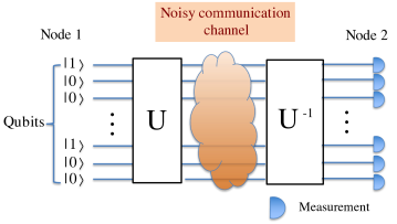
The general form of a QDL protocol follows (Fig. 1).
-
1.
In advance, Alice and Bob publicly agree upon a set of unitary matrices in , say . Each unitary matrix identifies a basis in the Hilbert space, which is obtained by applying the unitary to the standard computational basis. Denote as the elements of the computational basis. Then the unitary identifies the basis .
-
2.
To send information to Bob, first Alice uses a secret key of bits to choose one particular unitary transformation, i.e., one particular basis in the agreed set of bases.
-
3.
Alice selects basis vectors, from the chosen basis and use them as a code to send bits of classical information through the quantum channel. This encoding of classical information into a quantum system is described by the classical-quantum state
(1) where is the classical variable encoded by Alice, which is represented by a set of orthogonal vectors in a dummy quantum system.
In this work we assume that different code words have equal probability. As the goal of the protocol is to extend an initial secret key into a longer one, using equally probable code words is a natural assumption. It makes the analysis of the QDL protocol easier, although it can be relaxed [21, 22].
The code words prepared by Alice are then sent to Bob through a quantum channel described as a completely positive and trace preserving map that transforms Alice’s system into Bob’s system . The channel maps the state in Eq. (1) into
| (2) |
We ask a QDL protocol to have the properties of correctness and security.
Correctness. The property of correctness requires that, if Bob knows the secret key used by Alice to chose the code words, then he is able to decode reliably. For example, if the channel is noiseless, then is the identity map and
| (3) |
In this case, Bob can simply apply the inverse unitary, , followed by a measurement in the computational basis. In this way, Bob can decode with no error for any . If the channel is noisy, Alice and Bob can still communicate reliably at a certain rate of bits per channel use. This is possible by using error correction at any rate below the channel capacity, [23]. Here denotes the mutual information between the input variable and the output of Bob’s measurement , given the shared secret key . Notice that here we need classical error correction and not quantum error correction, as the goal of Alice and Bob is to exchange classical information and not quantum information. Furthermore, we apply post facto error correction, as it is commonly done in quantum key distribution [24], in which error correcting information is sent independently on a classical authenticated public channel.
We emphasize the importance of the assumption that the adversary has no quantum memory for the security of post facto error correction. This assumption guarantees that a potential eavesdropper has already measured their share of the quantum system when the error correction information is exchanged on a public channel. If bits of error correcting information are communicated on a public channel, then the eavesdropper cannot learn more than bits of information about the message 222To see that the public channel for error correction does not render the protocol insecure, we note that Eve’s additional information about the secret key is bounded by classical information theory as follows. Let be the message sent by Alice, the output of Eve’s measurement, and the mutual information. After error correction, Eve obtains a bit string . Hence, we need to consider the mutual information . It follows from the property of incremental proportionality [2] of the mutual information that , where is the entropy of . This implies that, knowing after she measured the quantum system, Eve cannot learn more than bits about the message .. If instead the eavesdropper has a quantum memory with storage time , then Alice and Bob need to wait for a time larger than after the quantum signal have been transmitted and before proceeding with post facto error correction. In this work we assume that Alice and Bob know an upper bound on .
Security. The property of security requires that, if Bob does not know the secret key, he can obtain no more than a negligibly small amount of information about Alice’s input variable . To clarify this, consider that, if Bob does not know the secret key used by Alice, then his description of the classical quantum state is the average of Eq. (2),
| (4) |
In QDL, the security is quantified using the accessible information [2, 6] (or similar quantities [7, 21, 25]). Recall that the accessible information is defined as the maximum information that Bob can obtain about by measuring his share of the state , that is,
| (5) |
where the optimization is over the measurement maps on system , and is the mutual information between and the outcome of the measurement. The security property can be defined in different ways, depending on how the state is chosen. Here we consider a strong notion of QDL [3] and put
| (6) |
This is equivalent to saying that the information remains encrypted even if Bob is capable of accessing the quantum resource directly without the mediation of a noisy channel. The data processing inequality [23] then implies that the protocol is secure for noisy channels too. In conclusion, we say that the protocol is secure if , with arbitrarily small. This means that only a negligible fraction of the information can be obtained by measuring the quantum state without having knowledge of the secret key.
Intuitively, we expect that the larger , the smaller the accessible information. This intuition has been proven true using tools from large deviation theory and coding theory [6, 7, 4]. The mathematical characterization of a QDL protocol consists in obtaining, for given , an estimate of the minimum integer such that there exist choices of bases that guarantee .
Finally, the net secret key rate that can be established between Alice and Bob, through a noisy communication channel , is
| (7) |
where is the efficiency of error correction, and we have subtracted the initial amount of secret bits shared between Alice and Bob. We emphasise that the mutual information depends on the particular noisy channel, whilst is universal. The noisier the channel, the smaller , which accounts for the error correction overhead. The factor accounts for the fact that practical error correction requires more overhead than expected in theory.
3 Multiphoton encoding
Let photons be sent into optical modes of an interferometer with at most one photon per input mode. The input modes evolve into , with the unitary transformation describing the interferometer:
| (8) |
A passive multi-mode interferometer realises a unitary transformation that preserves the total photon number. The set of all possible transformations that can be realised in this way defines the group of linear passive optical (LOP) unitary transformations, which is isomorphic to the -dimensional unitary group (see e.g. Ref. [20]). By Shur’s lemma, the group of LOP unitaries has irreducible representations in the subspaces with definite photon number. For applications to photonic QDL, the representation with photon has been studied in previous works [10, 3]. This representation has the unique feature of being the fundamental representation of . However, representations with higher photon number that we are considering here are no longer the fundamental representation.
The output from the interferometer prior to photo-detection can be expanded in the photon-number basis:
| (9) |
where denotes a photon-number configuration with photons in the -th mode and its amplitude.
The aim of this paper is to characterize a particular family of QDL protocols, where information is encoded into optical modes using photons. We define the code words by putting photons on different modes, with no more than one photon per mode.
In this way we obtain a code book that contains code words, whereas the overall Hilbert space defined by photons on modes has dimensions (this includes states with more than one photon in a given mode). For example, with modes and photon, we have the code words , , , . With photons, we instead obtain the code words , , , , , .
The two users, Alice and Bob, are linked via an optical communication channel that allows Alice to send optical modes at the time. Initially, we assume the channel is noiseless. Later we will extend to the case of a noisy channel. The goal of the protocol, which is shown schematically in Fig. 1, is for Alice and Bob to expand an initial secret key of bits into a longer one.
For given and , Alice defines a code book by choosing a subset of code words from . The code book is publicly announced. We denote the code words as , with . To encrypt these code words, Alice applies an -mode LOP unitary transformation from a set of elements . The unitary is determined by the value of her secret key of bits. We recall that any LOP unitary can be realised as a network of beam splitters and phase shifters [26, 27].
We can directly verify the correctness property for a noiseless communication channel. In this case, Bob, who knows the secret key, applies and measures by photo-detection. He is then able to decrypt bits of information with no error. This implies that Alice and Bob can establish a key of bits for each round of the protocol.
To characterise the secrecy of the QDL protocol, we need to identify the minimum key size . This is the task that we accomplish in the following sections below.
4 Preliminary considerations
Before presenting our main results, we need to introduce some notation and preliminary results. First, consider the following state,
| (10) |
which is defined by taking the average over the LOP unitary acting on a state . Here denotes the expectation value over the invariant measure (i.e., the Haar measure) on the group LOP unitary transformations acting on optical modes. The choice of the invariant measure is somewhat arbitrary and other measures can be used, see e.g. Ref. [28]. In Eq. (10), is a vector in the code book . By symmetry, is independent of .
Consider, as an example, the manifold of states with photons over modes. We denote as the subspace spanned by vectors that have at most one photon in each mode, i.e., the linear span of , , , . The subspace is characterised by a specific pattern describing how photons are distributed on the modes. Another subspace is , which is spanned by the vectors , …, etc. Finally, there exists one more photon pattern for modes and photons, denoted as . The corresponding subspace is spanned by the vectors , , , . We label the different subspaces by . These definitions naturally extend to any and . In general, a patter of photons over modes is identified as , for integers such that . We denote as the corresponding subspace, and is the projector onto .
By symmetry, the state is block-diagonal in the subspaces , i.e.,
| (11) |
We are particularly interested in the smallest coefficient in this expansion,
| (12) |
which can be computed numerically for given and . Examples are shown in Table 1. The results of our numerical estimations suggest that the minimum is always achieved for the pattern , i.e., when each mode contains at most photon. An analytical expression for is given in Ref. [29],
| (13) |
Supported by the results of our numerical search, we formulate the following conjecture:
Conjecture 1
We have used this conjecture to produce the plot in Fig. 3. If the number of modes is much larger than the number of photons squared, , the probability that two or more photons occupy a given mode is highly suppressed. In this limit, we have (see Appendix D).
| Photon occupancy pattern | |||
|---|---|---|---|
The other quantity we are interested in is
| (15) |
where the maximum is over a generic -photon vector , and is a vector in the code book . Again, because of symmetry, is independent of . Note that quantifies how much the transition probability changes when a random unitary is applied. In the regime of , an analytical bound can be computed and we obtain . This is discussed in Appendix D.
For generic values of and , we estimate numerically. To do that, we first expand the generic state as
| (16) |
where identifies a subspace with given photon occupancy pattern, and labels the basis vectors within. By symmetry, the following identities hold:
| (17) |
and
| (18) |
This implies
| (19) |
and
| (20) |
where the second inequality is an application of Cauchy-Schwarz.
In conclusion we obtain the upper bound
| (21) |
Compared with the definition in Eq. (15), to compute this upper bound we only need to consider the basis vectors . Furthermore, by symmetry, the quantities and are independent of . The expression in Eq. (21) is therefore suitable to be evaluated numerically. The penalty that we pay for this simplification is the multiplication by a factor . Some examples are shown in Table 2. More numerical estimations of are shown in Appendix D. Our numerical search suggests that the maximum in Eq. (21) is achieved for . Supported by these numerical results, we formulate the following conjecture:
Conjecture 2
The maximum in Eq. (21) is obtained when all photons occupy the same mode, i.e., for . This yields
| (22) |
where
| (23) |
This conjecture is used to produce Fig. 3.
| Photon pattern | |||
|---|---|---|---|
| 6 | |||
| 6 | |||
| (40,2) | 6 | ||
| (40,3) | 8 | ||
5 Results
Our main result is an estimate of the minimum key size that guarantees that the accessible information is of order . This estimate is expressed in terms of the parameters and introduced in Section 4.
Proposition 1
Consider the QDL protocol described in Section 3, which encodes bits of information using photons over modes. For any , and for any , there exist choices of linear optics unitaries such that , where
| (24) |
and . Recall that is the dimension of the Hilbert space with photons over modes, and is the number of states with no more than one photon per mode.
The parameters and depend on the particular values of and . We identify three regimes for and :
- 1.
-
2.
In the regime where (the no-collision regime), and (see Appendix D.
- 3.
We can write Eq. (24) as
| (25) |
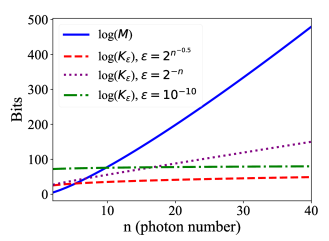
where the functions and scale as . For illustration, Fig. 2 shows and an estimate of as functions of . To obtain the plot, we have chosen and used the limiting values for the parameters and .
Note that, as is expected to be sufficiently small, this estimate for the secret key size is useful only in the limit of asymptotically large , i.e., when one encodes information using asymptotically many modes and photons. This is certainly not the regime one is willing to test in an experimental demonstration of QDL.
The QDL protocol outperforms the classical one-time pad when , for some reasonably small value of . Some numerical examples are in Fig. 2, which show the gap between and increases with increasing number of modes and photons. For example, for , , , and , we obtain and . This shows explicitly that we can achieve information theoretical security with a private key shorter than the message if and are large enough.
Scaling up the communication protocol: in a practical communication scenario, not only one signal, but a large number of signals are sent from Alice to Bob through a given quantum communication channel. Consider a train of channel uses, where Alice encodes a classical variable into tensor-product code words of the form
| (26) |
where each component is a state of photons over modes. Over channel uses, the total number of code words is denoted as , and the code rate is . Similarly, Alice applies local unitaries to these code words,
| (27) |
for a total number of allowed unitaries acting on channel uses. We denote as the outputs of channel uses received by Bob. The security condition on the mutual information then reads .
Corollary 1
For any , and for any , there exist choices of local unitaries upon channel uses such that , where
| (28) |
The minimum secret key consumption rate then reads
| (29) |
Corollary 1 allows us to estimate the net secret key rate as the difference between the code rate and the secret key consumption rate,
| (30) |
where conjecture 1 implies . If , then the QDL is successful in beating the classical one-time pad and generates a secret key at a rate of bits per channel use larger than the key consumption rate of bits.
We can compare these results with the classical one-time pad encryption as well as previously known QDL protocols. We consider the three parameters that characterise symmetric key encryption: the length of the initial secret key, the length of the message, and the security parameter . Classical one-time pad requires for perfect encryption (). Therefore, the comparison with QDL makes sense in the regime where can be made arbitrary small. In this regime, we can then say that a QDL protocol beats the classical one-time pad if .
The QDL protocol that has up to now the largest gap between and was proposed by Fawzi et al. in Ref. [7]. This protocol requires an initial key of constant size for any sufficiently large . This is obtained by using random unitaries in the -dimensional Hilbert space, and therefore requires a universal quantum computer acting on a large Hilbert space.
Proposition 1 shows that there exist QDL protocols with . Comparing with Ref. [7], the length of the secret key has an overhead proportional to
| (31) |
The advantage with respect to Ref. [7] is that the encryption only requires linear optical passive unitaries. For and large, using the Stirling approximation we obtain
| (32) |
which becomes negligibly small in the limit of diluted photons, .
Corollary 1 shows the existence of QDL protocols for channel uses where a secret key of allows us to encrypt , where in the limit that , and the constant depends on the particular choice of the parameters and . Note that in these protocols the secret key length is not constant, but scales as the message length . Although they have the same scaling, we can still have in some regime. Despite being less efficient in terms of key use, the advantage of these protocols is that they only need linear optics passive unitaries acting on a small number of photons and modes, i.e., and can be chosen finite and small. For example, for photons over modes, we obtain and . From table 4 we also obtain the numerical estimates . Putting , we obtain the following estimate for the asymptotic rate of secret key consumption,
| (33) |
This shows explicitly that less than bits of secret key are used to encrypt a message of bits. Therefore, the net key generation rate in this case is
| (34) |
In Section 8 we consider the effect of photon loss in terms of the net rate per mode, .
6 Proof of Proposition 1
We prove the proposition using a random-coding argument. We show that a random choice of the code and of the set of scrambling unitaries leads, with high probability, to a QDL protocol that satisfies the security property.
The code book of cardinality is randomly chosen by sampling from the code book of cardinality . We put . For , we expect that the code words are all distinct up to terms of second order in . Therefore the code words encode bits of information.
The sender Alice first prepares a state , then applies a linear optics unitary . The unitary is chosen among a pool of elements according to a secret key of bits. We choose the pool of unitaries by drawing unitaries i.i.d. according to the uniform Haar measure on the group of linear optics unitary transformations on modes. If the receiver does not know the secret key, the state is described by the density operator
| (35) |
Given the classical-quantum state
| (36) |
Bob attempts to extract information from this state by applying a measurement . Such a measurement is characterised by the POVM elements , where ’s are unit vectors and such that , with the identity operator. Without loss of generality we can consider rank-one POVM only [2]. The output of this measurement is a random variable with probability density
| (37) |
and conditional probability
| (38) |
The accessible information is the maximum mutual information between and :
| (39) |
where
| (40) |
This yields
| (41) |
Note that the accessible information is written as the difference of two entropy-like quantities. The rationale of the proof is to show that for large enough, and for random choices of the unitaries and of the code words, both terms in the curly brackets are arbitrarily close to
| (42) |
for all vectors , where is as in Eq. (10). This in turn implies that the accessible information can be made arbitrarily small. To show this we exploit the phenomenon of concentration towards the average of the sum of i.i.d. random variables. This concentration is quantified by concentration inequalities.
We now proceed along two parallel directions.
First, we apply the matrix Chernoff bound [30] to show that is close to . In particular the matrix Chernoff bound implies that the inequality
| (43) |
holds true up to a failure probability
| (44) |
This in turn implies
| (45) |
uniformly for all . The details are presented in Appendix A below.
Second, we apply a tail bound from A. Maurer [31] to show that
| (46) |
up to a failure probability
| (47) |
The above applies uniformly to all unit vectors and for almost all values of . This implies that
| (48) |
In conclusion, we obtain that, up to a probability smaller than ,
| (49) |
The details are presented in Appendix B.
Putting the above results in Eq. (45) and (49) into Eq. (6) we finally obtain
| (50) |
Recall that is a probability distribution. Therefore, as the average is always smaller that the maximum, we obtain
| (51) |
where can be computed as shown in Section 4.
The above bound on the accessible information is not deterministic, but the probability that it fails can be made arbitrary small provided is large enough (see Appendix C for details). This probability is bounded away from if
| (52) |
and
| (53) |
The size of critically depends on the factor , which determines the convergence rate of the Maurer tail bound. How to estimate this coefficient is the subject of Appendix D.
7 Proof of Corollary 1
Consider a train of channel uses. Alice encodes information using code words of the form , where each component is chosen randomly and independently from the code book , which has cardinality . Each -fold code word is uniquely identified by the multi-index . We put , where is a small positive constant.
First Alice encodes information across signal uses using the code words , then she applies local unitaries to scramble them. The set of possible unitaries is made of elements. These unitaries are chosen by sampling identically and independently from the Haar measure on the unitary group of linear optical passive unitary transformations on modes. Note that, whereas is arbitrary large, the number of modes in each signal transmission will be kept constant and relatively small. Also, the number of photons per channel use is fixed and equal to .
The accessible information is then formally equivalent to the one in Eq. (6):
| (54) |
where for each ,
| (55) | ||||
| (56) | ||||
| (57) |
This in particular implies
| (58) |
and therefore
| (59) | ||||
| (60) |
To bound we can first decompose a generic vector as , where define a basis of product vectors. We can then apply the Cauchy-Schwarz inequality, as shown in Section 4, to obtain the upper bound .
In conclusion, we can straightforwardly repeat the proof of Section 6 with these new parameters. This yields that, for any arbitrarily small , the bound
| (61) |
holds with non-zero probability provided that (recall that )
| (62) |
Finally, in the limit of , and since , we obtain
| (63) |
8 Noisy channels
A practical communication protocol needs to account for loss and noise in the communication channel. This requires us to introduce error correction in the classical post-processing. We address this issue here and show that the structure of our proof encompasses a large class of error correcting protocols.
In the case of a noisy and lossy channel, Alice and Bob can still use the channel by employing error correction. Error correction comes with an overhead that reduces the maximum communication rate from (the maximum amount of information that can be conveyed through a noiseless channel) to , where is the mutual information given that both Alice and Bob know the secret key .
The amount of loss and noise in the communication channel can be experimentally determined with the standard tools of parameter estimation, a routine commonly employed in quantum key distribution. This in turn allows Alice and Bob to quantify .
In principle, error correction allows Alice and Bob to achieve a communication rate arbitrarily close to . In practice, however, we can only partially achieve this goal. To model this fact, one usually introduce the error correction efficiency factor . Putting this together with Corollary 1, we obtain our estimate for the net rate of the protocol:
| (64) |
where a positive net rate expresses the fact that the QDL protocol allows us to expand the initial secret key into a longer one.
As an example, consider the case where Alice and Bob communicate through a lossy optical channel. The efficiency factor represents the probability that a photon sent by Alice is detected by Bob, including both channel losses and detector efficiency. The mutual information between Alice and Bob can be computed explicitly (see Appendix E for detail). We obtain :
| (65) | ||||
| (66) |
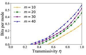
Fig. 3 shows the quantity , i.e., the number of bits per mode, for , for a pure loss channel with transmissivity . The plot is obtained assuming Conjectures 1 and 2. This shows that QDL can be demonstrated experimentally with loss and inefficient detectors. In particular, higher loss can be tolerated by increasing the number of optical modes. Note that the values for the number of photons and modes used to obtain this figure have been achieved experimentally in Ref. [32].
9 Conclusions
The phenomenon of Quantum Data Locking (QDL) represents one of the most remarkable separations between classical and quantum information theory. In classical information theory, information-theoretic encryption of a string of bits can be only made by exploiting a secret key of at least bits. This is realised, for example, by using a one-time pad. By contrast, QDL shows that, if information is encoded into a quantum system of matter or light, it is possible to encrypt bits of information with a secret key of bits. QDL is a manifestation of the uncertainty principle in quantum information theory [8, 9].
Initial works on QDL have focused on abstract protocols defined in a Hilbert space of asymptotically large dimensions. More recent works have extended QDL to system of relatively small dimensions that are transmitted through many uses of a communication channel. This approach allowed to incorporate error correction and led to one of the first experimental demonstrations of QDL in an optical setup [13].
Inspired by Boson Sampling [33, 34], in this work we have further extended QDL to a setup where information is encoded using multiple photons scattered across many modes, and processed using linear passive optics. The extension of QDL to multiphoton states is technically challenging due to role played by higher-order representations of the unitary group.
Our protocols for multiphoton QDL has the potential to data-lock more bits per optical mode, hence can achieve a higher information density. Experimental realisations of our protocols are challenging but feasible with state-of-the-art technology. This is suggested by recent results in photon generation and advances in integrated linear optics, e.g., Ref. [32] reported interference of photons across modes.
Several works have attempted to apply the physical insights of Boson Sampling in a quantum information framework beyond its defining problem. In this paper, we provide a protocol for quantum cryptography based on the physics of Boson Sampling. We have presented an information-theoretic proof that a linear-optical interferometer, fed with multiple photons, is useful for quantum cryptography. The security of our protocol does not rely on the classical computational complexity of Boson Sampling. Therefore it holds for any number of modes and photon number . The security proof is based on QDL and random coding techniques. We have shown that our protocol remains secure when we use classical error correction to protect the channel against photon loss and other errors. It is therefore a scalable and efficient protocol for quantum cryptography.
References
- Shannon [1949] Claude E Shannon. Communication theory of secrecy systems. Bell system technical journal, 28(4):656–715, 1949.
- DiVincenzo et al. [2004] David P. DiVincenzo, Michał Horodecki, Debbie W. Leung, John A. Smolin, and Barbara M. Terhal. Locking classical correlations in quantum states. Phys. Rev. Lett., 92:067902, Feb 2004. doi: 10.1103/PhysRevLett.92.067902.
- Guha et al. [2014] Saikat Guha, Patrick Hayden, Hari Krovi, Seth Lloyd, Cosmo Lupo, Jeffrey H. Shapiro, Masahiro Takeoka, and Mark M. Wilde. Quantum enigma machines and the locking capacity of a quantum channel. Phys. Rev. X, 4:011016, Jan 2014. doi: 10.1103/PhysRevX.4.011016.
- Lupo and Lloyd [2014] Cosmo Lupo and Seth Lloyd. Quantum-locked key distribution at nearly the classical capacity rate. Phys. Rev. Lett., 113:160502, Oct 2014. doi: 10.1103/PhysRevLett.113.160502.
- Lupo [2015] Cosmo Lupo. Quantum data locking for secure communication against an eavesdropper with time-limited storage. Entropy, 17(5):3194–3204, 2015.
- Hayden et al. [2004] Patrick Hayden, Debbie Leung, Peter W Shor, and Andreas Winter. Randomizing quantum states: Constructions and applications. Communications in Mathematical Physics, 250(2):371–391, 2004. doi: 10.1007/s00220-004-1087-6.
- Fawzi et al. [2013] Omar Fawzi, Patrick Hayden, and Pranab Sen. From low-distortion norm embeddings to explicit uncertainty relations and efficient information locking. Journal of the ACM, 60:44, 2013. doi: 10.1145/2518131.
- Wehner and Winter [2010] Stephanie Wehner and Andreas Winter. Entropic uncertainty relations—a survey. New Journal of Physics, 12(2):025009, feb 2010. doi: 10.1088/1367-2630/12/2/025009.
- Coles et al. [2017] Patrick J. Coles, Mario Berta, Marco Tomamichel, and Stephanie Wehner. Entropic uncertainty relations and their applications. Rev. Mod. Phys., 89:015002, Feb 2017. doi: 10.1103/RevModPhys.89.015002.
- Lloyd [2013] Seth Lloyd. Quantum enigma machines. arXiv preprint arXiv:1307.0380, 2013.
- Winter [2017] Andreas Winter. Weak locking capacity of quantum channels can be much larger than private capacity. Journal of Cryptology, 30(1):1–21, Jan 2017. ISSN 1432-1378. doi: 10.1007/s00145-015-9215-3.
- Lupo and Lloyd [2015] Cosmo Lupo and Seth Lloyd. Quantum data locking for high-rate private communication. New Journal of Physics, 17(3):033022, 2015. doi: 10.1088/1367-2630/17/3/033022.
- Lum et al. [2016] Daniel J. Lum, John C. Howell, M. S. Allman, Thomas Gerrits, Varun B. Verma, Sae Woo Nam, Cosmo Lupo, and Seth Lloyd. Quantum enigma machine: Experimentally demonstrating quantum data locking. Phys. Rev. A, 94:022315, Aug 2016. doi: 10.1103/PhysRevA.94.022315.
- Liu et al. [2016] Yang Liu, Zhu Cao, Cheng Wu, Daiji Fukuda, Lixing You, Jiaqiang Zhong, Takayuki Numata, Sijing Chen, Weijun Zhang, Sheng-Cai Shi, Chao-Yang Lu, Zhen Wang, Xiongfeng Ma, Jingyun Fan, Qiang Zhang, and Jian-Wei Pan. Experimental quantum data locking. Phys. Rev. A, 94:020301, Aug 2016. doi: 10.1103/PhysRevA.94.020301.
- Notaros et al. [2017] Jelena Notaros, Jacob Mower, Mikkel Heuck, Cosmo Lupo, Nicholas C. Harris, Gregory R. Steinbrecher, Darius Bunandar, Tom Baehr-Jones, Michael Hochberg, Seth Lloyd, and Dirk Englund. Programmable dispersion on a photonic integrated circuit for classical and quantum applications. Opt. Express, 25(18):21275–21285, Sep 2017. doi: 10.1364/OE.25.021275.
- Cozzolino et al. [2019] Daniele Cozzolino, Beatrice Da Lio, Davide Bacco, and Leif Katsuo Oxenløwe. High-dimensional quantum communication: Benefits, progress, and future challenges. Advanced Quantum Technologies, 2(12):1900038, 2019. doi: 10.1002/qute.201900038.
- He et al. [2017] Yu He, X. Ding, Z.-E. Su, H.-L. Huang, J. Qin, C. Wang, S. Unsleber, C. Chen, H. Wang, Y.-M. He, X.-L. Wang, W.-J. Zhang, S.-J. Chen, C. Schneider, M. Kamp, L.-X. You, Z. Wang, S. Höfling, Chao-Yang Lu, and Jian-Wei Pan. Time-bin-encoded boson sampling with a single-photon device. Phys. Rev. Lett., 118:190501, May 2017. doi: 10.1103/PhysRevLett.118.190501.
- Zhong et al. [2018] Han-Sen Zhong, Yuan Li, Wei Li, Li-Chao Peng, Zu-En Su, Yi Hu, Yu-Ming He, Xing Ding, Weijun Zhang, Hao Li, Lu Zhang, Zhen Wang, Lixing You, Xi-Lin Wang, Xiao Jiang, Li Li, Yu-Ao Chen, Nai-Le Liu, Chao-Yang Lu, and Jian-Wei Pan. 12-photon entanglement and scalable scattershot boson sampling with optimal entangled-photon pairs from parametric down-conversion. Phys. Rev. Lett., 121:250505, Dec 2018. doi: 10.1103/PhysRevLett.121.250505.
- Wang et al. [2019a] Hui Wang, Jian Qin, Xing Ding, Ming-Cheng Chen, Si Chen, Xiang You, Yu-Ming He, Xiao Jiang, L. You, Z. Wang, C. Schneider, Jelmer J. Renema, Sven Höfling, Chao-Yang Lu, and Jian-Wei Pan. Boson sampling with 20 input photons and a 60-mode interferometer in a -dimensional hilbert space. Phys. Rev. Lett., 123:250503, Dec 2019a. doi: 10.1103/PhysRevLett.123.250503.
- Aniello et al. [2006] Paolo Aniello, Cosmo Lupo, and Mario Napolitano. Exploring representation theory of unitary groups via linear optical passive devices. Open Sys. & Inf. Dynamics, 13:415, 2006. doi: 10.1007/s11080-006-9023-1.
- Dupuis et al. [2013] Frédéric Dupuis, Jan Florjanczyk, Patrick Hayden, and Debbie Leung. The locking-decoding frontier for generic dynamics. Proc. R. Soc. A, 469:2159, 2013. doi: 10.1098/rspa.2013.0289.
- Zixin et al. [2020] Huang Zixin, Pieter Kok, and Cosmo Lupo. Protecting the output of a quantum computer with random circuit samplers. arXiv:quant-ph/2003.11470, 2020.
- Wilde [2013] Mark M Wilde. Quantum information theory. Cambridge University Press, 2013.
- Bennett et al. [1988] C. H. Bennett, G. Brassard, and J.-M. Robert. Privacy amplification by public discussion. SIAM J. Comput., 17:210, 1988.
- Adamczak [2017] Radosław Adamczak. Metric and classical fidelity uncertainty relations for random unitary matrices. Journal of Physics A: Mathematical and Theoretical, 50(10):105302, feb 2017. doi: 10.1088/1751-8121/aa5662.
- Reck et al. [1994] Michael Reck, Anton Zeilinger, Herbert J. Bernstein, and Philip Bertani. Experimental realization of any discrete unitary operator. Phys. Rev. Lett., 73(1):58–61, July 1994. doi: 10.1103/PhysRevLett.73.58.
- Clements et al. [2016] William R. Clements, Peter C. Humphreys, Benjamin J. Metcalf, W. Steven Kolthammer, and Ian A. Walmsley. Optimal design for universal multiport interferometers. Optica, 3(12):1460–1465, Dec 2016. doi: 10.1364/OPTICA.3.001460.
- Lupo et al. [2014] Cosmo Lupo, Mark M. Wilde, and Seth Lloyd. Robust quantum data locking from phase modulation. Phys. Rev. A, 90:022326, Aug 2014. doi: 10.1103/PhysRevA.90.022326.
- Drummond et al. [2016] P. D. Drummond, B. Opanchuk, L. Rosales-Zárate, M. D. Reid, and P. J. Forrester. Scaling of boson sampling experiments. Phys. Rev. A, 94:042339, Oct 2016. doi: 10.1103/PhysRevA.94.042339.
- Ahlswede and Winter [2002] Rudolf Ahlswede and Andreas Winter. Strong converse for identification via quantum channels. IEEE Transactions on Information Theory, 48(3):569–579, 2002. doi: 10.1109/18.985947.
- Maurer [2003] Andreas Maurer. A bound on the deviation probability for sums of non-negative random variables. J. Inequalities in Pure and Applied Mathematics, 4(1):15, 2003.
- Wang et al. [2019b] Hui Wang, Jian Qin, Xing Ding, Ming-Cheng Chen, Si Chen, Xiang You, Yu-Ming He, Xiao Jiang, L. You, Z. Wang, C. Schneider, Jelmer J. Renema, Sven Höfling, Chao-Yang Lu, and Jian-Wei Pan. Boson sampling with 20 input photons and a 60-mode interferometer in a -dimensional Hilbert space. Phys. Rev. Lett., 123:250503, Dec 2019b. doi: 10.1103/PhysRevLett.123.250503.
- Aaronson and Arkhipov [2011] Scott Aaronson and Alex Arkhipov. The computational complexity of linear optics. In Proceedings of the forty-third annual ACM symposium on Theory of computing, pages 333–342. ACM, 2011. doi: 10.1145/1993636.1993682.
- Aaronson and Arkhipov [2014] Scott Aaronson and Alex Arkhipov. Boson Sampling is far from uniform. Quantum Information & Computation, 14(15-16):1383–1423, 2014. doi: http://arXiv:1309.7460
- Scheel [2004] Stefan Scheel. Permanents in linear optical networks. doi: https://arxiv.org/abs/quant-ph/0406127, 2004.
Appendix A Matrix Chernoff bounds
The matrix Chernoff bound states the following (this formulation can be obtained directly from Theorem 19 of Ref. [30]):
Theorem 1
Let be i.i.d. -dimensional Hermitian-matrix-valued random variables, with , , and . Then, for :
| (67) |
where denotes the probability that the proposition is true, and .
Note that for we have
| (68) |
and for
| (69) |
First consider the collection of code words . We apply the Chernoff bound to the independent random variables . Note that these operators are defined in a -dimensional Hilbert space. For we then have
| (70) |
Consider now the collection of random variables . We assume that they are bounded by . We apply again the Chernoff bound:
| (71) |
Thus the total probability reads
| (72) | ||||
| (73) |
Putting we obtain
| (74) |
In conclusion we have obtained that, up to a probability smaller than ,
| (75) |
Appendix B The Maurer tail bound
We also need to apply the following concentration inequality due to A. Maurer [31]:
Theorem 2
Let be i.i.d. non-negative real-valued random variables, with and finite first and second moments, . Then, for any we have that
| (76) |
For any given and , we apply this bound to the random variables
| (77) |
Note that (see Section 4)
| (78) |
and
| (79) |
The application of the Maurer tail bound then yields
| (80) |
where
| (81) |
Note that, by symmetry, is independent of . The calculation of is presented in Appendix D.
B.1 Extending to almost all code words
The probability bound in Eq. (80) is about one given value of . Here we extend it to distinct values :
| (82) |
where we have used the fact that for different values of the variables are statistically independent (recall that the code words are chosen randomly and independently). Second, we extend to all possible choices of code words. This amount to a total of events. Applying the union bound we obtain
| (83) |
This implies that, up to a probability smaller than , for at least values of . This in turn yields
| (84) |
Putting :
| (85) | ||||
| (86) | ||||
| (87) |
B.2 Extending to all vectors
The final step is to extend the result to all unit vectors. This can be done by exploiting the notion of -net. A -net is a discrete and finite set of vectors on the unit sphere such that for any unit vector there exists an element in the -net such that
| (88) |
It is known that there exist -nets with no more than elements [6], where is the Hilbert space dimension. We put , therefore the size of the net is . Applying the union bound on Eq. (83) we then obtain
| (89) |
To conclude, we put and obtain that, uniformly in ,
| (90) |
The probability that this bound is violated is smaller than (recall that )
| (91) | ||||
| (92) | ||||
| (93) |
Appendix C Probability of failure
The above concentration inequalities allow us to prove that the protocol is secure up a to certain probability. The bad event that the protocol is not secure occurs when either Eq. (45) or (49) is violated. The probability of the bad event is then smaller the sum of the corresponding probabilities, which are given in Eq. (74) and (93) respectively. We therefore have
| (94) | ||||
| (95) |
This probability is bounded away from if
| (96) |
and
| (97) |
Appendix D Estimating the factor
The goal of this Appendix is to estimate the factor that determines the secret key consumption rate. The objective is therefore to evaluate the first and second moments of the random variable
| (98) |
where restricted to be a vector in the single-occupancy subspace , which is our code space. A generic state can be written as
| (99) |
We can apply the Cauchy-Schwarz inequality as shown in Section 4. This yields (see Eq. (21)):
| (100) |
By symmetry, the quantities
| (101) |
do depend on but not on the particular vector in the subspace , nor on the code word . Therefore for each , can be computed numerically and in turn obtain an estimate for the upper bound on the speed of convergence
| (102) |
Following the notation from Ref. [35], let be the matrix whose matrix elements are those of the original matrix with row indices , and column indices .
| (103) |
The object denotes a matrix whose entries are taken from the matrix , and whose row index occurs times, and whose column index occurs times. For example
| (104) | ||||
| (105) |
Using Eq. (105), we can calculate Eq. (100) for a particular photon occupancy pattern.
We numerically compute for different photon patterns for between and , examples are given in Table 2 and 3. Note that the number of configurations to search over grows exponentially with , and thus the search becomes infeasible with high . The calculations were performed in Python by computing the permanents of submatrices of the unitaries generated from the Haar measure. The expectation value is taken by averaging over runs. We observe that the highest value of is achieved when all the photons populate only one mode. To make the calculation feasible, we conjecture (Conjecture 2) that this is also true for higher ; in this case, the computation can be performed much more efficiently because the submatrices have repeated rows. This conjecture has been used to produce the plots in Fig. 3. We repeat the calculation for to , where the results are shown in Table 4.
We now consider the regime of in which we can neglect photon bunching. Therefore, we compute the first and second moments of the random variable
| (106) |
This is a little less general than (98) because is not a generic vector in . In fact and identify two sets of modes, with labels and , respectively. This corresponds to photon-counting on the modes, which as we know, maps onto sub-matrix of the unitary matrix :
| (107) |
The random variable is the modulus square of the permanent of :
| (108) |
where the sum is over all the permutations .
To further explore the statistical properties of the permanent, it is useful to recall that a given entry of a random unitary is itself distributed approximately as an complex Gaussian variable with zero mean and variance . If instead we consider a submatrix of size the entries are with good approximation independent Gaussian variables as long as [33]. This means that the entries are approximately distributed as i.i.d. complex Gaussian variables with zero mean and variance . Using this fact we can compute the first and second moments of .
| (109) |
since the non-zero terms are given by .
From Lemma 56 of Ref. [33], the fourth moment of the permanent can be computed as
| (110) |
In conclusion, we have obtained
| (111) |
From which it follows,
| (112) |
| Photon pattern | ||
|---|---|---|
| (20,4) | 5.44 | |
| 8.91 | ||
| 6.60 | ||
| 8.38 | ||
| 13.31 | ||
| (20,5) | 5.45 | |
| 8.44 | ||
| 12.13 | ||
| 7.80 | ||
| 10.50 | ||
| 6.50 | ||
| 16.93 | ||
| (20,6) | 5.34 | |
| 7.26 | ||
| 12.86 | ||
| 8.72 | ||
| 7.77 | ||
| 15.89 | ||
| 6.16 | ||
| 13.42 | ||
| 10.50 | ||
| 9.50 | ||
| 26.34 | ||
| (20,8) | 15.81 | |
| 7.30 | ||
| 18.04 | ||
| 11.11 | ||
| 5.98 | ||
| 7.95 | ||
| 10.91 | ||
| 11.03 | ||
| 19.18 | ||
| 9.09 | ||
| 4.92 | ||
| 24.34 | ||
| 34.86 |
| Photon pattern | ||
| (30,4) | 5.92 | |
| 9.97 | ||
| 7.28 | ||
| 9.47 | ||
| 15.07 | ||
| (30,5) | 6.12 | |
| 10.10 | ||
| 14.63 | ||
| 9.30 | ||
| 12.88 | ||
| 7.44 | ||
| 19.12 | ||
| (30,6) | 6.11 | |
| 9.03 | ||
| 16.74 | ||
| 11.19 | ||
| 20.82 | ||
| 7.29 | ||
| 17.44 | ||
| 13.98 | ||
| 9.72 | ||
| 11.99 | ||
| 33.20 | ||
| (30,8) | 23.70 | |
| 9.63 | ||
| 27.56 | ||
| 17.58 | ||
| 7.63 | ||
| 10.10 | ||
| 17.84 | ||
| 15.70 | ||
| 35.89 | ||
| 12.80 | ||
| 5.82 | ||
| 34.43 | ||
| 61.69 |
| Photon pattern | ||
|---|---|---|
| (40,4) | 6.09 | |
| 10.60 | ||
| 7.59 | ||
| 9.81 | ||
| 15.91 | ||
| (40,5) | 6.51 | |
| 11.01 | ||
| 16.08 | ||
| 10.02 | ||
| 13.93 | ||
| 8.050 | ||
| 20.18 | ||
| (40,6) | 6.68 | |
| 10.03 | ||
| 19.82 | ||
| 13.04 | ||
| 23.15 | ||
| 8.16 | ||
| 20.40 | ||
| 15.57 | ||
| 10.91 | ||
| 13.88 | ||
| 35.95 | ||
| (40,8) | 32.65 | |
| 12.24 | ||
| 47.54 | ||
| 23.89 | ||
| 9.09 | ||
| 14.25 | ||
| 20.99 | ||
| 21.25 | ||
| 36.11 | ||
| 17.05 | ||
| 6.484 | ||
| 56.08 | ||
| 67.49 |
| Photon pattern | ||
|---|---|---|
| 40.84 | ||
| 53.87 | ||
| 73.45 | ||
| (30,10) | 111.5 | |
| (30,11) | 124.6 | |
| (30,12) | 164.7 | |
| (30,13) | 201.4 | |
| (40,9) | 114.5 | |
| (40,10) | 161.2 | |
| (40,11) | 207.2 | |
| (40,12) | 259.7 | |
| (40,13) | 422.1 |
| Photon pattern | ||
|---|---|---|
| (60,4) | 16.63 | |
| (60,6) | 43.59 | |
| (60,8) | 112.6 | |
| (60,10) | 230.2 | |
| (60,12) | 500.4 | |
| (60,14) | 722.7 | |
| (60,16) | 1877 | |
| (60,18) |
Appendix E Mutual information for a pure loss channel
For a lossy channel with transmissivity , the mutual information between Alice and Bob (given that Bob knows the secret key) can be computed explicitly. We assume that Bob measures by photo-detection. First, we note that, since the key is independent on the both and , we have .
If Alice sends one particular code words containing photons, Bob will get photons with probability . This is uniquely identified if Bob measures by photo-detection by detection events. There exists possible measurement outputs of this kind. Therefore the conditional entropy is
| (113) | ||||
| (114) | ||||
| (115) |
where is the probability of code words .
Now consider that Bob obtains a certain combination of detection events over modes. This output is compatible with input code words sent by Alice. As the total number of code words is , the probability of obtaining a given combination of detections is
| (116) |
Note that the total number of possible outputs is , therefore we have
| (117) | ||||
| (118) | ||||
| (119) |
Finally we obtain:
| (120) | ||||
| (121) |
