Robust regression based on shrinkage estimators

Abstract

A robust estimator is proposed for the parameters that characterize the linear regression problem. It is based on the notion of shrinkages, often used in Finance and previously studied for outlier detection in multivariate data. A thorough simulation study is conducted to investigate: the efficiency with normal and heavy-tailed errors, the robustness under contamination, the computational times, the affine equivariance and breakdown value of the regression estimator. Two classical data-sets often used in the literature and a real socio-economic data-set about the Living Environment Deprivation of areas in Liverpool (UK), are studied. The results from the simulations and the real data examples show the advantages of the proposed robust estimator in regression.

Keywords: robust regression, robust Mahalanobis distance, shrinkage estimator, outliers.

1 Introduction

Linear regression problems are widely used in numerous fields. The diversity of data for which the model is used poses a problem since not all available methods work well for high dimension, high sample size, not all are sufficiently resistant to the presence of anomalous values, and are computationally feasible at the same time. Consider the linear regression model:

$$y_{i}=\alpha+\mathbf{x}_{i}^{t}\boldsymbol{\beta}+\epsilon_{i}$$ (1)

for $i=1,...,n$, where $n$ is the sample size, $\alpha$ is the unknown intercept, $\boldsymbol{\beta}$ is the unknown $(p\times 1)$ vector of regression parameters, and the error terms $\epsilon_{i}$ are i.i.d and also independent from the $p$-dimensional explanatory variables $\mathbf{x}_{i}$ (often also called regressor variables or carriers). The classical approach to estimate the parameters of the model is the ordinary least squares (OLS) estimator of Gauss and Legendre, which minimizes the sum of squared residuals:

$$\hat{\boldsymbol{\beta}}_{OLS}=\underset{\boldsymbol{\beta}}{argmin}\sum_{i=1}^{n}(y_{i}-\mathbf{x}_{i}^{t}\boldsymbol{\beta})^{2}$$ (2)

The problem with OLS is that a single unusual observation can have a large impact on the estimate. Through all these past three decades there have been different approaches attempting the robustification of the procedure, although there is no consensus that establishes which method is recommended in practical situations. OLS estimator can be expressed as follows. Denote the joint variable of the response and carriers as $\mathbf{z=(x,y)}$. Denote the location of $\mathbf{z}$ by $\boldsymbol{\mu}$ and the scatter matrix by $\Sigma$. Partitioning $\boldsymbol{\mu}$ and $\Sigma$ yields the notation:

$$\begin{matrix}\boldsymbol{\mu}=\begin{pmatrix}\boldsymbol{\mu}_{x}\\ \mu_{y}\end{pmatrix}&,&\Sigma=\begin{pmatrix}\Sigma_{xx}&\Sigma_{xy}\\ \Sigma_{yx}&\Sigma_{yy}\end{pmatrix}\end{matrix}$$ (3)

Traditionally they are estimated by the empirical mean $\hat{\boldsymbol{\mu}}$ and the empirical covariance matrix $\hat{\Sigma}$. OLS estimators of $\boldsymbol{\beta}$ and the intercept $\alpha$ can be written as functions of the components of $\boldsymbol{\hat{\mu}}$ and $\hat{\Sigma}$, namely

$$\hat{\boldsymbol{\beta}} =\hat{\Sigma}_{xx}^{-1}\hat{\Sigma}_{xy},\quad\quad\hat{\alpha}=\hat{\mu}_{y}-\hat{\boldsymbol{\beta}}^{t}\hat{\boldsymbol{\mu}}_{x}$$ (4)

The drawback is that the classical sample estimators are sensitive to the presence of outliers. Instead, robust estimators should be used. The contribution of this paper is to propose robust estimators based on shrinkage to be used in Equation 4 for estimating the regression parameters (a similar idea can be seen in Maronna and Morgenthaler [1986] and Croux et al. [2003]. These estimators based on shrinkage have shown advantages when they were used for defining a robust Mahalanobis distance to detect outliers in the multivariate space [Cabana et al., 2019] and in the present paper, the performance in linear regression is studied, through simulations and real data examples. The notion of shrinkage is used in Finance and Portfolio optimization, and it provides a trade-off between low bias and low variance (Ledoit and Wolf [2003b], Ledoit and Wolf [2003a], Ledoit and Wolf [2004], DeMiguel et al. [2013]), and in case of covariance matrices, well-conditioned estimates are obtained, a fact that is of relevance when inversion of the matrix is at stake, as is the case now.

Furthermore, a real socio-economic example that explains the Living Environment Deprivation (LED) index of areas in Liverpool (UK) through remote sensing data, is studied. The data was previously used in Arribas-Bel et al. [2017] where two machine learning approaches were investigated in this context: Random Forest (RF) and Gradient Boost Regressor (GBR). In this paper we study the proposed robust regression approach with the LED index data and found out that it provides an improvement of the cross-validated $R^{2}$ and mean squared error with respect to classical OLS and both machine learning techniques RF and GBR, while maintaining the advantage of interpretability, which is a weakness that RF and GBR have.

The paper is organized as follows. Section 2 shows a state-of-the-art review of the most used methods for robust regression in the literature. In Section 3, the alternative robust method based on shrinkage is proposed. The approach is compared with the others by means of simulations. The description of the simulation scenarios is shown in Section 4. In Section 5 the efficiency is studied with normal errors and heavy-tailed distributed erros. In Section 6, the robustness and the computational performance are investigated in presence of contamination. Section 7 shows the equivariance property studied by means of simulations and the breakdown value is shown in Section 8. On the other hand, real data examples are considered in Section 9. Finally, in Section 10 some conclusions are provided.

2 State of the art

The efficiency and breakdown point (bdp) are two traditionally used criteria to compare the existing robust methodologies. The first one because OLS has the smallest variance among unbiased estimates when the errors are normally distributed and there are no outliers. This means that, in this scenario, OLS has maximum efficiency. Thus, the relative efficiency of the robust estimate compared to OLS when the error distribution is exactly normal and the data is clean, is often considered as a measure to study the performance of the methods and to compare them with each other. The bdp measures the proportion of outliers an estimate can tolerate. Usually, the definition of finite sample bdp is used [Donoho and Huber, 1983]. Given any sample $\mathbf{z}=(\mathbf{z}_{1},...,\mathbf{z}_{n})$, with $\mathbf{z}_{i}=(\mathbf{x}_{i},y_{i})$, where $\mathbf{x}_{i}$ is of dimension $1\times p$, for all $i=1,...,n$, denote by $T(\mathbf{z})$ an estimate of the parameter $\boldsymbol{\beta}$. Let $\widetilde{\mathbf{z}}$ be the corrupted sample where any $q$ of the original points of $\mathbf{z}$ are replaced by arbitrary outliers. Then the finite sample bdp $\gamma^{*}$ is defined as:

$$\gamma^{*}(T,\mathbf{z})=\underset{1\leq q\leq n}{min}\{\frac{q}{n}:\underset{\widetilde{z}}{sup}\ ||T(\widetilde{\mathbf{z}})-T(\mathbf{z})||=\infty\}$$ (5)

where $||\cdot||$ is the Euclidean norm. The asymptotic bdp is understood as the limit of the finite sample bdp when $n$ goes to infinity. Intuitively, the maximum possible asymptotic bdp is $1/2$ because if more than half of the observations are contaminated, it is not possible to distinguish between the background data and the contamination [Leroy and Rousseeuw, 1987]. OLS has a finite sample bdp of $1/n$ and asymptotic bdp of $0$.

A first proposal of a robust estimate in regression came from Edgeworth [1887] who proposed to replace the squared residuals in the definition of Equation 2 by their absolute value. It was called Least Absolute Deviation (LAD) or $L_{1}$ estimate and it was more resistant than OLS against outliers in the response variable $y$, but still couldn’t resist outlying values in the carriers. These kind of outliers are called leverage points, which may have a large effect on the fit. Thus, the finite sample bdp of LAD is $1/n$.

The next idea was made by Huber [1964] (also see Huber [1973] and Huber [1981]) who proposed to replace the least-square criterion by a robust loss function $\rho(\cdot)$ of the residuals. It was called M-estimator, which was more efficient than LAD. However, the finite sample bdp of both LAD and M tend to 0, because of the possibility of leverage points [Maronna et al., 2006]. Besides, the method implies one first decision: which loss function $\rho$ should be used. Huber’s loss or the Tukey’s bisquare functions are common choices, but there are no rules for which should be selected when we are dealing with real data. Furthermore, they depend on a constant that determines the efficiency of the estimator, and this might be a problem as well in practice. Due to the vulnerability of M-estimators, the generalized M-estimators (also called GM-estimators) were proposed, and the problem of recognizing leverage points was solved, but it could not distinguish between “good” and “bad” leverage points, and the bdp decreases as the dimension $p$ of the data increases.

Siegel [1982] proposed a near $50\%$ bdp technique, the Least Median of Squares (LMS), which minimizes the median of the squared residuals. However, the procedure had a disadvantage in the order of convergence (Rousseeuw [1984], Rousseeuw and Croux [1993]). Another approach was proposed by Rousseeuw [1983], called Least Trimmed Squares (LTS) and it consisted on minimizing the sum of the $h$ ordered squared residuals, where $h$ is the proportion of trimming. Usually $h=n/2+1$ results in a bdp of $50\%$ and better convergence rate than LMS. The problem is LTS suffers in terms of low efficiency relative to OLS [Stromberg et al., 2000].

Robust regression by means of S-estimator came by hands of Rousseeuw and Yohai [1984]. The method has greater asymptotic efficiency than LTS, but depending on the specification of some constants. Croux et al. [1994] proposed the generalized S-estimator (GS-estimator) to improve the efficiency, but again there was a constant to define, which depends on $n$ and $p$.

MM-estimators were proposed by Yohai [1987] and consisted in three basic stages. For the initial step, a consistent robust estimate of the regression parameters with high bdp but not necessarily high efficiency, was needed. In practice the typical initial estimators are LMS or S-estimate with Huber or bisquare functions. Playing with the constants necessary for the estimators, MM-estimates can attain high efficiency without affecting its bdp. However the author recognize in Yohai [1987] that if the constant that handles the efficiency is increased, then the estimates get more sensitive to outliers.

Maronna and Morgenthaler [1986] and Croux et al. [2003] proposed another idea based on using robust estimators in the expression for OLS estimates from Equation 4. They propose to use the multivariate M-estimators and the S-estimator (method S from now on), respectively.

The robust and efficient weighted least square estimator (REWLSE) was proposed by Gervini and Yohai [2002]. The method simultaneously achieve maximum bdp and full efficiency under Gaussian errors. The idea is to use hard rejection weights (0 or 1) calculated from an initial robust estimator. The cut-off depends on the distribution of the standardized absolute residuals, and because of these adaptive cut-off, the method is asymptotically equivalent to OLS and hence its full asymptotic efficiency.

In summary, all these least squares alternatives exhibit some drawbacks. Some are robust to outliers in the response, but not resistant to leverage points, or could not distinguish between good or bad leverage. A maximum bdp is difficult to achieve maintaining high efficiency. MM-estimator, method S and REWLSE estimator seem to be the best alternatives because of their high bdp and high asymptotic efficiency. It is important to note that even though some mentioned estimators have high bdp, their computation is challenging specially in case of large data-sets or high dimension. That is why approximate algorithms have to be used, which are usually based on taking a number of subsamples and iterate. This fact translates in worse performance about consistency and bdp than the exact theoretical estimator would have had. It gets worse with the increase of the sample size $n$ or the dimension $p$ of the samples (Stromberg et al. [2000], Hawkins and Olive [2002]). Furthermore, with all these methods there always have to be a decision of which tuning constant choose, or which function of the residuals use, or which first initial estimator use. The problem becomes complicated with all of these decisions in case of real data.

3 Shrinkage reweighted regression

In this paper, robust estimators of location and scatter matrix based on the notion of shrinkage, are used in Equation 4. The notion of shrinkage relies on the fact that “shrinking” an estimator $\hat{E}$ of a parameter towards a target estimator $\hat{T}$, would help to reduce the estimation error because it is a trade-off between a low bias estimator and a low variance estimator. According to James and Stein [1992], under general conditions, there exists a shrinkage intensity $\eta$, so the resulting shrinkage estimator would contain less estimation error than $\hat{E}$.

$$\hat{E}_{Sh}=(1-\eta)\hat{E}+\eta\hat{T}$$ (6)

Let $\mathbf{x}=\{\mathbf{x}_{\cdot 1},...,\mathbf{x}_{\cdot p}\}$ be the $n\times p$ data matrix with $n$ being the sample size and $p$ the number of variables. In Cabana et al. [2019], the shrinkage estimator $\hat{\boldsymbol{\mu}}_{Sh}$ is proposed as a robust estimator of central tendency.

$$\hat{\boldsymbol{\mu}}_{Sh}=(1-\eta)\hat{\boldsymbol{\mu}}_{MM}+\eta\nu_{\boldsymbol{\mu}}\mathbf{e}$$ (7)

where $\hat{\boldsymbol{\mu}}_{MM}$ is the multivariate $L_{1}-$median, which is a robust and highly efficient estimator of location (Lopuhaa and Rousseeuw [1991], Vardi and Zhang [2000], Oja [2010]). The target estimator was $\nu_{\boldsymbol{\mu}}\mathbf{e}$ , where $\mathbf{e}$ is the $p$-dimensional vector of ones, analogous as in DeMiguel et al. [2013]. The scaling factor $\nu_{\boldsymbol{\mu}}$ and the intensity $\eta$ are obtained minimizing the expected quadratic loss. The solution can be found in Proposition 2 from Cabana et al. [2019]. On the other hand, the authors also propose an adjusted special comedian matrix $\hat{S}_{Sh}$, based on the classical definition of comedian from Falk [1997], and with it a shrinkage estimator for the covariance matrix can be obtained.

$$\hat{S}_{Sh}=2.198\cdot(median((\mathbf{x}_{\cdot j}-(\boldsymbol{\hat{\mu}}_{Sh})_{j})(\mathbf{x}_{\cdot t}-(\boldsymbol{\hat{\mu}}_{Sh})_{t}))$$ (8)

The idea came from the fact that the comedian matrix is a robust alternative for the covariance matrix, but in general it is not positive (semi-)definite [Falk, 1997], and with the shrinkage approach applied to the comedian, a robust and well-conditioned estimate is obtained (Ledoit and Wolf [2003b], Ledoit and Wolf [2003a], Ledoit and Wolf [2004], DeMiguel et al. [2013]). The shrinkage estimator will be:

$$\hat{\Sigma}_{Sh}=(1-\eta)\hat{S}_{Sh}+\eta\nu_{\Sigma}I$$ (9)

The optimal expression for the parameters $\eta$ and $\nu_{\Sigma}$ is described in Cabana et al. [2019] in Proposition 3. Furthermore, the authors used the robust estimators of location $\hat{\boldsymbol{\mu}}_{Sh}$ and covariance matrix $\hat{\Sigma}_{Sh}$ based on shrinkage to define a robust Mahalanobis distance that had the ability to discover outliers with high precision in the vast majority of cases in the simulation scenarios studied in the paper, with both gaussian data and with skewed or heavy-tailed distributions. The behavior under correlated and transformed data showed that the approach was approximately affine equivariant. With highly contaminated data it is shown that the method had high breakdown value even in high dimension.

In the present paper, the estimation of the regression parameters using these robust estimators based on shrinkage in Equation 4, is proposed. Consider the joint vector $\mathbf{z=(x,y)}$ with $\boldsymbol{\mu}$ and $\Sigma$ the location and covariance matrix of $\mathbf{z}$ described in Equation 3. Now let us call the shrinkage estimators $\hat{\boldsymbol{\mu}}_{Sh}$ and $\hat{\Sigma}_{Sh}$ for the location and covariance matrix of $\mathbf{z}$, the initial shrinkage robust estimators of central tendency and covariance matrix of $\mathbf{z}$, respectively. Now let us define the associated robust squared Mahalanobis distance for each observation $\mathbf{z}_{i}$, with $i=1,...,n$:

$$d^{2}(\mathbf{z}_{i})=(\mathbf{z}_{i}-\hat{\boldsymbol{\mu}}_{Sh})^{t}\hat{\Sigma}_{Sh}^{-1}(\mathbf{z}_{i}-\hat{\boldsymbol{\mu}}_{Sh})$$ (10)

Let $w_{i}=w(d^{2}(\mathbf{z}_{i}))$ be a weight function depending on the robust squared Mahalanobis distance. The second step is to obtain $\hat{\boldsymbol{\mu}}_{Sh}^{SW}$ and $\hat{\Sigma}_{Sh}^{SW}$, the shrinkage weighted estimator for the mean and covariance matrix:

$$\hat{\boldsymbol{\mu}}_{Sh}^{SW} =\frac{\sum_{i=1}^{n}w_{i}\mathbf{z}_{i}}{\sum_{i=1}^{n}w_{i}},\quad\hat{\Sigma}_{Sh}^{SW}=\frac{\sum_{i=1}^{n}w_{i}(\mathbf{z}_{i}-\hat{\boldsymbol{\mu}}_{Sh}^{SW})(\mathbf{z}_{i}-\hat{\boldsymbol{\mu}}_{Sh}^{SW})^{t}}{\sum_{i=1}^{n}w_{i}}$$ (11)

Based on $\hat{\boldsymbol{\mu}}_{Sh}^{SW}$ and $\hat{\Sigma}_{Sh}^{SW}$ we can obtain $\hat{\boldsymbol{\beta}}^{SW}$ and $\hat{\alpha}^{SW}$ which are initial estimates for the regression parameters. Let us call them shrinkage weighted (SW) regression estimators:

$$\hat{\boldsymbol{\beta}}^{SW} =(\hat{\Sigma}_{Sh}^{SW})_{xx}^{-1}(\hat{\Sigma}_{Sh}^{SW})_{xy},\quad\hat{\alpha}^{SW}=(\hat{\boldsymbol{\mu}}_{Sh}^{SW})_{y}-(\hat{\boldsymbol{\beta}}^{SW})^{t}(\hat{\boldsymbol{\mu}}_{Sh}^{SW})_{x}$$ (12)

The SW error’s scale estimate is:

$$\hat{\sigma}^{SW}=(\hat{\Sigma}_{Sh}^{SW})_{yy}-(\hat{\boldsymbol{\beta}}^{SW})^{t}(\hat{\Sigma}_{Sh}^{1})_{xx}\hat{\boldsymbol{\beta}}^{SW}$$

The third step is reweighting, taking into consideration the residuals based on the SW regression estimators:

$$r_{i}^{SW}=y_{i}-(\hat{\boldsymbol{\beta}}^{SW})^{t}\mathbf{x}_{i}-\hat{\alpha}^{SW}$$ (13)

Define the Mahalanobis distance for the SW residuals:

$$d(r_{i}^{SW})=((r_{i}^{SW})^{t}(\hat{\sigma}^{SW})^{-1}r_{i}^{SW})^{1/2}$$ (14)

Let $wr_{i}=w(d^{2}(r_{i}^{SW}))$ a weighting function that depends on the Mahalanobis distance of the SW residuals. Define $\mathbf{u}_{i}=(\mathbf{x}_{i}^{t},1)^{t}$ and obtain:

$$\hat{\boldsymbol{\varphi}}^{SR}=((\hat{\boldsymbol{\beta}}^{SR})^{t},\hat{\alpha}^{SR})^{t}=\left(\sum_{i=1}^{n}wr_{i}\mathbf{u}_{i}\mathbf{u}_{i}^{t}\right)^{-1}\sum_{i=1}^{n}wr_{i}y_{i}\mathbf{u}_{i}$$ (15)

Then, $\hat{\boldsymbol{\varphi}}^{SR}=\left(\left(\hat{\boldsymbol{\beta}}^{SR}\right)^{t},\hat{\alpha}^{SR}\right)^{t}$ are the shrinkage reweighted (SR) regression estimators.

For the weighting functions the inverse of the squared robust Mahalanobis distance was studied, but the indicator function in both cases (as in Rousseeuw et al. [2004]) had improved performance. The first weight function is $w_{i}=w(d^{2}(\mathbf{z}_{i}))=I(d^{2}(\mathbf{z}_{i})\leq q_{1})$, which assigns weight 1 to the $\mathbf{z}_{i}$, for $i=1,...,n$, with a robust squared Mahalanobis distance less than certain quantile $q_{1}$ of the chi-square distribution with $p+1$ degrees of freedom. The second weighting function is $wr_{i}=w(d^{2}(r_{i}^{SW}))=I(d^{2}(r_{i}^{SW})\leq q_{2})$, which assigns weight 1 to the residuals $r_{i}^{SW}$ with a Mahalanobis distance less than certain quantile $q_{2}$ of the chi-square distribution with $1$ degree of freedom.

The quantiles

$$q_{1}=\chi^{2}_{p+1,1-\delta_{1}}\quad\text{and}\quad q_{2}=\chi^{2}_{1,1-\delta_{2}}$$ (16)

depend on the significance levels $\delta_{1}$ and $\delta_{2}$, for which $0.025$ and $0.01$ are chosen, respectively, as in Rousseeuw et al. [2004], because those are the classical choices for the threshold to detect outliers [Leroy and Rousseeuw, 1987].

4 Simulation structure

In this section a simulation study is conducted to investigate the performance of the proposed SR regression estimator and compare it with OLS and some of the previously mentioned robust regression methods: LTS, MM, method S and REWLSE. The simulations were done in Matlab: OLS with the fitlm function, LTS with the ltsregres function from LIBRA library (see Verboven and Hubert [2005]) considering the default option for the proportion of trimming which is $h=n/2+1$ and the default fraction of outliers the algorithm should resist which is equal to 0.75, MM with the MMreg function from FSDA toolbox (see Riani et al. [2012]), with default values for the nominal efficiency: 0.95 and the rho function to weight the residuals as the bisquare which uses Tukey’s functions, method S with the function SEst from the Discriminant Analysis Programme toolbox which computes biweight multivariate S-estimator for location and dispersion (see Ruppert [1992]) and REWLSE was computed with the functions the authors Gervini and Yohai [2002] kindly provided, with hard rejection weights and starting from an initial S-estimator.

Consider the linear regression model in matrix form:

$$\mathbf{y}=\alpha+X\boldsymbol{\beta}+\boldsymbol{\epsilon}$$ (17)

where $X$ is of size $n\times p$, $\boldsymbol{\beta}=(\beta_{1},...,\beta_{p})^{t}$ is the unknown $p\times 1$ vector of regression parameters, $\alpha$ the unknown intercept, and the errors $\boldsymbol{\epsilon}$ are i.i.d and independent from the carriers. The independent variables are distributed according to a multivariate standard Gaussian distribution $X\sim N(\mathbf{0}_{p},I_{p})$, where $\mathbf{0}_{p}$ is the $p-$dimensional vector of zeros and $I_{p}$ is the $p-$dimensional identity matrix. The simulation parameters are the following sets of dimension and sample size: $p=5$ with $n=20,30,50,100,1000$, $p=20$ with $n=80,100,200,500,5000$ and $p=30$ with $n=100,150,300,500,5000$. The simulations are repeated $M=1000$ times and each time the parameter estimates are drawn anew.

Three simulation scenarios are proposed, analogously as the simulation models found in the literature (Maronna and Morgenthaler [1986], Gervini and Yohai [2002], Croux et al. [2003], Rousseeuw et al. [2004], Agulló et al. [2008], Yu and Yao [2017]).

• The response is generated from a standard normal distribution $N(0,I)$, which corresponds to putting $\boldsymbol{\beta}=\mathbf{0}$ and $\alpha=0$ when gaussian errors are considered.

• The response is generated from a $t$-distribution with $3$ d.f, which corresponds to putting $\boldsymbol{\beta}=\mathbf{0}$ and $\alpha=0$ when $t_{3}$-distributed errors are considered.

• Normal errors as in [NE], but with probability $\delta$ the randomly selected observations in the independent variables were generated as $N(\lambda\sqrt{\chi^{2}_{p,0.99}},1.5)$ and the new response as $N(k\sqrt{\chi^{2}_{1,0.99}},1.5)$ where $\lambda,k=0,0.5,1,1.5,2,3,4,5,6,7,8,9,10$.

For the last simulation scenario [NEO], the levels of contamination considered were $\delta=10\%,20\%$. Note that if $\lambda=0$ and $k>0$ we obtain vertical outliers, if $\lambda>0$ and $k=0$ we obtain good leverage points and if $\lambda>0$ and $k>0$ we obtain bad leverage points. On the other hand, large values of $\lambda$ and $k$ produce extreme outliers, whereas small values produce intermediate outliers (see Croux et al. [2003] and Agulló et al. [2008]).

5 Efficiency

It is known that under simulation scheme [NE] the OLS estimator has maximum efficiency. The efficiency for each robust estimator, for finite samples, is calculated relative to OLS, considering the sum of squared deviations from the true coefficients and averaging over all repetitions. Consider the joint vector of regression parameters including the intercept $\boldsymbol{\varphi}=(\boldsymbol{\beta}^{t},\alpha)^{t}$, which has dimension $(p+1)\times 1$. For a certain robust method $R$, the finite sample efficiency for the joint estimator $\hat{\boldsymbol{\varphi}}_{R}$ is defined as:

$$\textrm{Eff}=\frac{1/M\sum_{m=1}^{M}||\hat{\boldsymbol{\varphi}}_{OLS}^{(m)}-\boldsymbol{\varphi}||_{2}^{2}}{1/M\sum_{m=1}^{M}||\hat{\boldsymbol{\varphi}}_{R}^{(m)}-\boldsymbol{\varphi}||_{2}^{2}}$$ (18)

Table 1 shows the simulated efficiencies relative to OLS, for the joint regression estimator $\hat{\boldsymbol{\varphi}}$ obtained with the proposed approach SR and the other robust regression methods, under simulation scheme [NE].

Table 1: Finite sample efficiency in case of normal errors, scenario [NE]

$p=5$	$n$	SR	LTS	S	REWLSE	MM
	20	0.9182	0.2352	0.2715	0.2346	0.2272
	30	0.9828	0.3486	0.4292	0.5026	0.4915
	50	0.9833	0.5061	0.5070	0.5129	0.5047
	100	0.9839	0.5870	0.7051	0.7441	0.7192
	1000	0.9859	0.7816	0.8691	0.9570	0.9159
$p=20$	80	0.9852	0.3763	0.6786	0.2809	0.2963
	100	0.9956	0.3973	0.7966	0.5028	0.4955
	200	0.9900	0.4971	0.8630	0.5811	0.8015
	500	0.9951	0.6163	0.8719	0.8737	0.8393
	5000	0.9981	0.6822	0.9461	0.9611	0.9068
$p=30$	100	0.9900	0.4458	0.5068	0.3622	0.2978
	150	0.9927	0.4699	0.5155	0.4347	0.5532
	300	0.9933	0.5110	0.5187	0.7524	0.5770
	500	0.9970	0.6467	0.8660	0.8479	0.8486
	5000	0.9980	0.6504	0.9646	0.9863	0.9781

In each row, bold letter represent the higher efficiency and italic letter represent the lowest efficiency. The results show that for a fixed dimension, when the sample size is increased, all methods improve the resulting finite sample efficiency. LTS is the method that behaves poorly even when the sample size increases. S, REWLSE and MM require large samples in order to have efficiencies greater than $90\%$. The proposed method SR has higher efficiency for every dimension and sample sizes considered.

In the simulation scenario [TE], OLS is not a maximum efficient estimator, due to the heavy-tailed errors. Therefore, Table 2 shows the mean squared errors (MSE) instead. The results show that, for all methods, large sample size translates into a decrease of the MSE, but method SR outperformed, in general, the other competitors.

Table 2: MSE in case of $t-$student distributed errors, scenario [TE]

$p=5$	$n$	SR	LTS	S	REWLSE	MM
	20	0.1499	0.2980	0.3634	0.4892	0.3193
	30	0.0579	0.0745	0.0662	0.1074	0.0713
	50	0.0304	0.0479	0.0409	0.0548	0.0322
	100	0.0114	0.0125	0.0150	0.0115	0.0116
	1000	0.0012	0.0016	0.0015	0.0017	0.0014
$p=20$	80	0.0244	0.0443	0.0293	0.1218	0.0881
	100	0.0126	0.0376	0.0228	0.0720	0.0364
	200	0.0107	0.0108	0.0114	0.0117	0.0118
	500	0.0033	0.0039	0.0036	0.0039	0.0034
	5000	0.0003	0.0004	0.0004	0.0003	0.0003
$p=30$	100	0.0202	0.0637	0.0375	0.1767	0.0855
	150	0.0110	0.0208	0.0157	0.0328	0.0240
	300	0.0052	0.0067	0.0074	0.0075	0.0055
	500	0.0032	0.0040	0.0038	0.0039	0.0033
	5000	0.0003	0.0005	0.0005	0.0003	0.0003

6 Robustness

Simulations to study the robustness are carried out, considering the third simulation scheme [NEO]. The most significant results are those consisting on dimensions $p=5,30$ with sample sizes $n=100,500$, respectively. The two statistical criteria used to compare the estimators from the different approaches were the squared Bias and the MSE for the estimated parameter vector $\hat{\boldsymbol{\beta}}$ and for the estimated intercept $\hat{\alpha}$ averaging over all $M$ simulation runs (see Gervini and Yohai [2002], Croux et al. [2003], Rousseeuw et al. [2004]). The following figures show, for each value of $\lambda$, the maximal value of MSE or Bias, obtained over all possible values of $k$.

$$MMSE_{\lambda}(\cdot) =max_{k\in\{0,...,10\}}MSE_{\lambda,k}(\cdot)$$

$$MBias_{\lambda}(\cdot) =max_{k\in\{0,...,10\}}Bias_{\lambda,k}(\cdot)$$ (19)

for each $\lambda\in\{0,...,10\}$. Figure 1 shows the $MMSE(\hat{\boldsymbol{\beta}}$), in case of low dimension $p=5$ with sample size $n=100$ and when the data is contaminated with a level of $10\%$. OLS shows high MSE when the data contains atypical observations, specially for vertical outliers and bad leverage observations associated with the first values of $\lambda$.

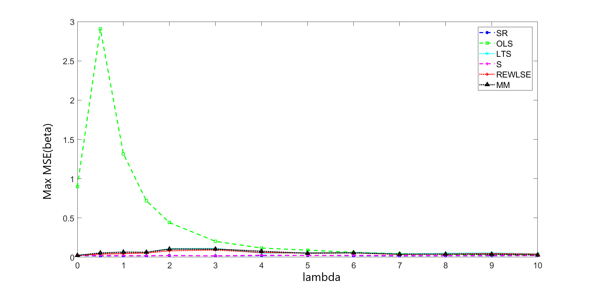
Figure 1: $MMSE(\hat{\boldsymbol{\beta}}$) with $p=5$, $n=100$, $\delta=10\%$.

If the previous image is zoomed, Figure 2, it can be seen that for vertical outliers, i.e. $\lambda=0$, all robust methods have similar MSE, but for the remaining values of $\lambda$, the smallest errors correspond to the proposed method SR and method S.

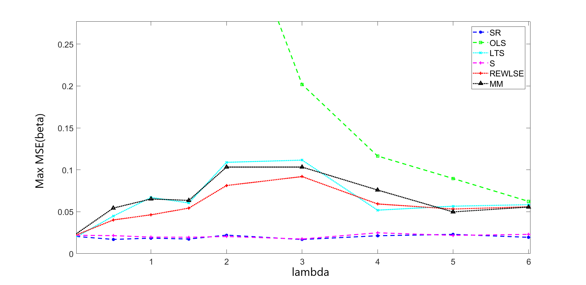
Figure 2: (Zoom) $MMSE(\hat{\boldsymbol{\beta}}$) with $p=5$, $n=100$, $\delta=10\%$.

For the MSE of $\hat{\alpha}$, and for the Bias of both $\hat{\alpha}$ and $\hat{\boldsymbol{\beta}}$, similar conclusions are obtained. In order to see these results from a different perspective, the error measures are summarized in a single graph for each dimension, sample size and contamination level. Figure 3 corresponds to $p=5$, $n=100$ and $\delta=10\%$. Each line represents a method. In the x-axis each number from 1 to 4 represents the maximum error measures: 1-MMMSE($\hat{\boldsymbol{\beta}}$), 2-MMMSE($\hat{\alpha}$), 3-MMBias($\hat{\boldsymbol{\beta}}$) and 4-MMBias($\hat{\alpha}$), over all possible values of $\lambda$.

$$MMMSE(\cdot) =max_{\lambda\in\{0,...,10\}}MMSE_{\lambda}(\cdot)$$

$$MMBias(\cdot) =max_{\lambda\in\{0,...,10\}}MBias_{\lambda}(\cdot)$$ (20)

for each $\lambda\in\{0,...,10\}$.

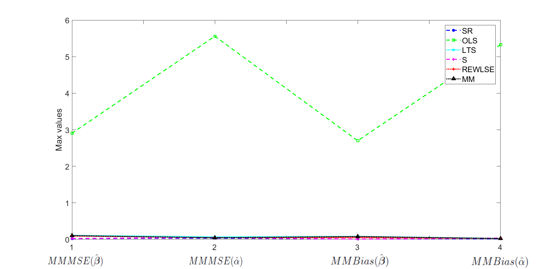
Figure 3: $MMMSE$, with $p=5$, $n=100$ and $\delta=10\%$.

Figure 4 is a zoom of the previous Figure 3. We can see in Figure 4 that in the majority of cases the proposed method SR has the lowest maximum MSE or Bias, except for one case in which method S has slightly lower maximum Bias($\hat{\boldsymbol{\beta}}$), but this happens only under low level of contamination.

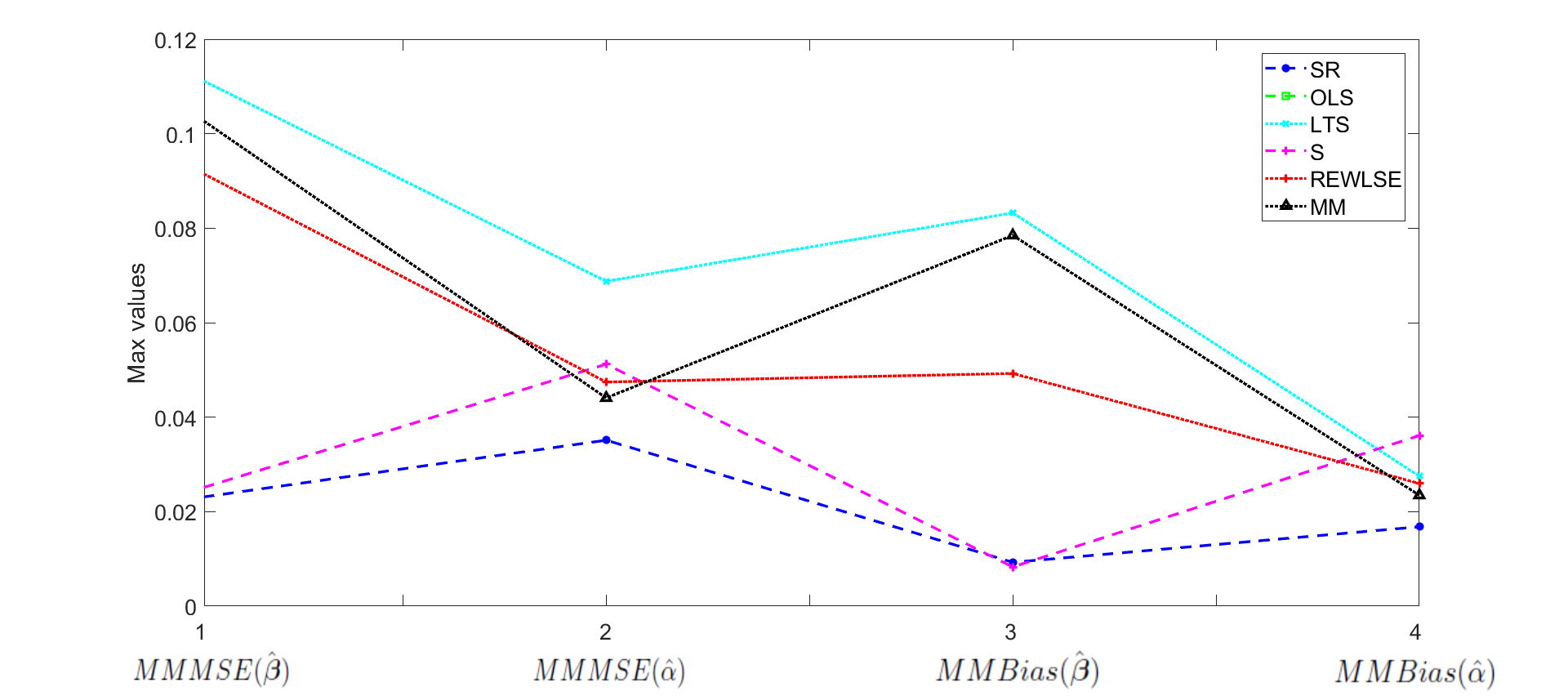
Figure 4: (Zoom) $MMMSE$, with $p=5$ and $\delta=10\%$.

When the contamination level $\delta$ increases to $20\%$, method S worsens its performance as it can be seen in Figure 5.

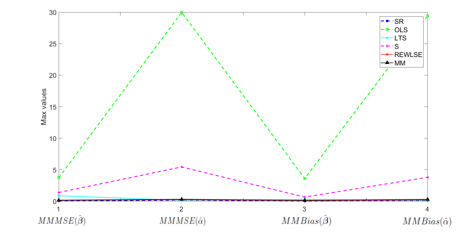
Figure 5: $MMMSE$, with $p=5$ and $\delta=20\%$.

Zoomed Figure 6 shows that, in case of higher contamination level, SR is the overall best performance method taking into account that although MSE($\hat{\alpha}$) and Bias($\hat{\alpha}$) are slightly lower for LTS, the MSE and Bias of the $\hat{\boldsymbol{\beta}}$ for LTS is much higher than SR, REWLSE and even MM estimator.

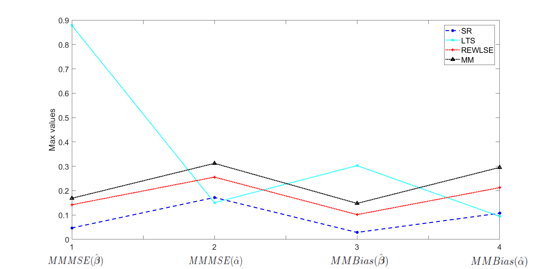
Figure 6: (Zoom) $MMMSE$, with $p=5$ and $\delta=20\%$.

Figure 7 shows that when the dimension is increased to $p=30$, and the contamination is $\delta=10\%$, the most affected methods are OLS and S. Method SR is the one that has the lowest maximum value for the MSE and Bias of both $\boldsymbol{\beta}$ and $\alpha$.

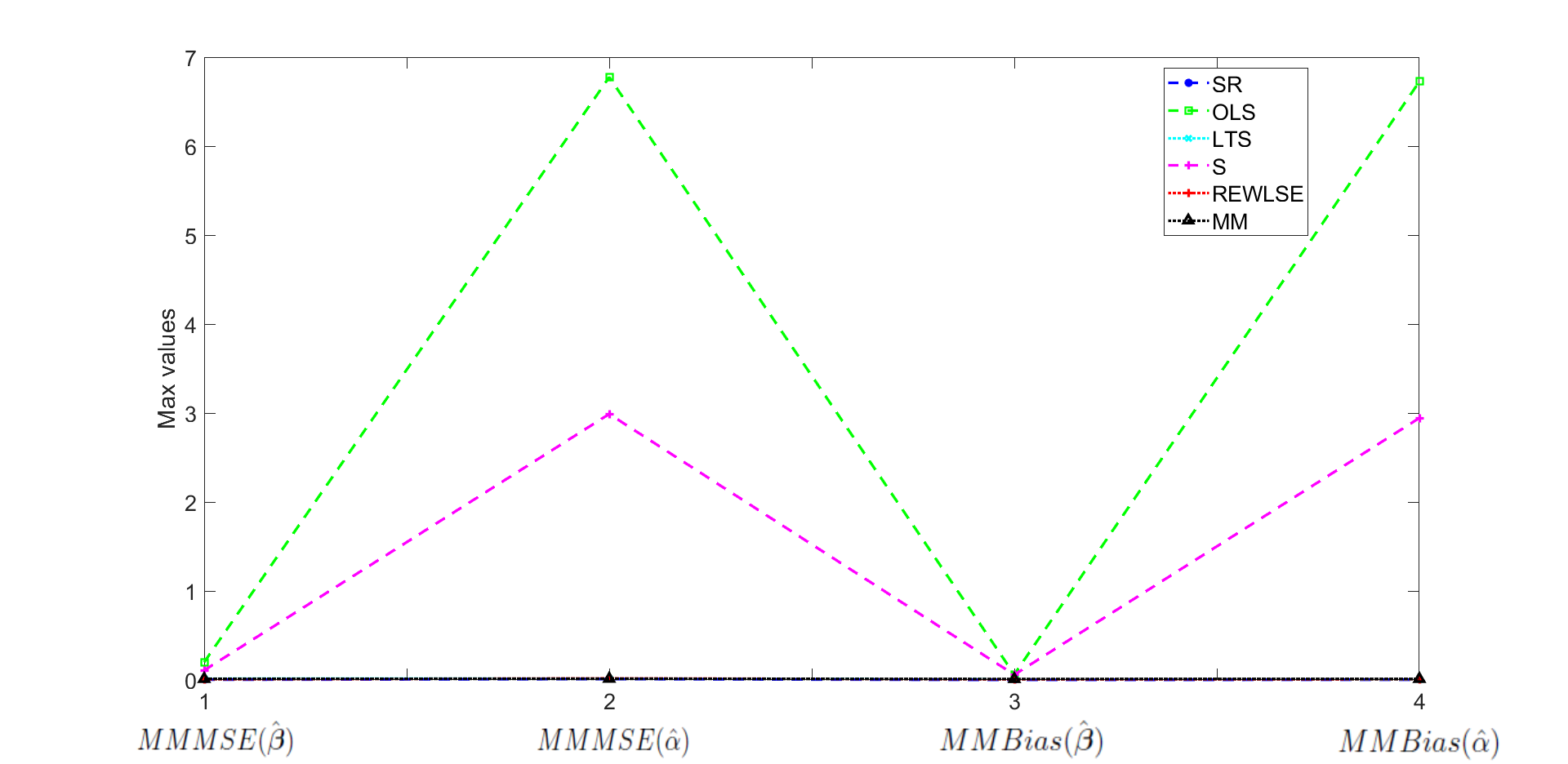
Figure 7: $MMMSE$, with $p=30$ and $\delta=10\%$.

Figure 8 is a zoom of Figure 7 so we can see the four methods with lowest errors. A similar situation happens in case of $\delta=20\%$ of contamination.

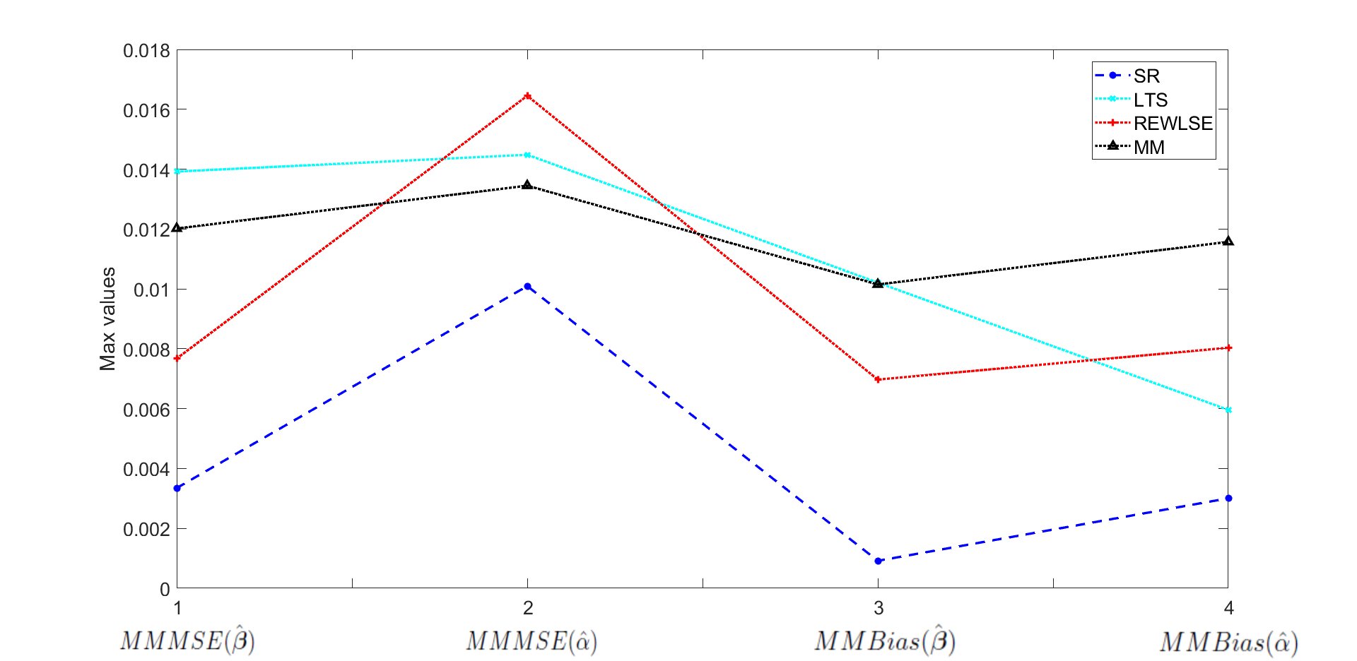
Figure 8: (Zoom) $MMMSE$, with $p=30$ and $\delta=10\%$.

Tables 3 - 6 show the numerical results. For each method, the maximum (across $\lambda$ and $k$) MSE and Bias for both $\hat{\boldsymbol{\beta}}$ and $\hat{\alpha}$ for each combination of the dimension $p$ and the contamination level $\delta$, is showed. In bold letter are the lowest error and in italic letter are the highest error after OLS. The results bear out with the ones from the Figures.

Table 3: MMMSE and MMBias of $\hat{\boldsymbol{\beta}}$ and $\hat{\alpha}$, for $p=5$ and $\delta=10\%$.

Method	MSE($\hat{\boldsymbol{\beta}}$)	MSE($\hat{\alpha}$)	BIAS($\hat{\boldsymbol{\beta}}$)	BIAS($\hat{\alpha}$)
OLS	2.9065	5.5593	2.7004	5.3280
SR	0.0230	0.0351	0.0093	0.0168
LTS	0.1116	0.0688	0.0832	0.0275
S	0.0249	0.0512	0.0083	0.0361
REWLSE	0.0919	0.0474	0.0493	0.0260
MM	0.1033	0.0441	0.0785	0.0235

Table 4: MMMSE and MMBias of $\hat{\boldsymbol{\beta}}$ and $\hat{\alpha}$, for $p=5$ and $\delta=20\%$.

Method	MSE($\hat{\boldsymbol{\beta}}$)	MSE($\hat{\alpha}$)	BIAS($\hat{\boldsymbol{\beta}}$)	BIAS($\hat{\alpha}$)
OLS	3.7360	29.9723	3.6101	29.4112
SR	0.0470	0.1720	0.0287	0.1075
LTS	0.8779	0.1508	0.3028	0.0947
S	1.3853	5.4441	0.6577	3.8112
REWLSE	0.1422	0.2556	0.1018	0.2124
MM	0.1688	0.3120	0.1478	0.2954

Table 5: MMMSE and MMBias of $\hat{\boldsymbol{\beta}}$ and $\hat{\alpha}$, for $p=30$ and $\delta=10\%$.

Method	MSE($\hat{\boldsymbol{\beta}}$)	MSE($\hat{\alpha}$)	BIAS($\hat{\boldsymbol{\beta}}$)	BIAS($\hat{\alpha}$)
OLS	0.1995	6.7748	0.0610	6.7250
SR	0.0033	0.0101	0.0009	0.0030
LTS	0.0139	0.0145	0.0102	0.0060
S	0.1079	2.9888	0.0584	2,9439
REWLSE	0.0077	0.0165	0.0070	0.0080
MM	0.0120	0.0134	0.0101	0.0116

Table 6: MMMSE and MMBias of $\hat{\boldsymbol{\beta}}$ and $\hat{\alpha}$, for $p=30$ and $\delta=20\%$.

Method	MSE($\hat{\boldsymbol{\beta}}$)	MSE($\hat{\alpha}$)	BIAS($\hat{\boldsymbol{\beta}}$)	BIAS($\hat{\alpha}$)
OLS	0.2317	25.5388	0.0639	25.3395
SR	0.0044	0.0596	0.0011	0.0554
LTS	0.0450	0.3952	0.0400	0.3677
S	0.1710	15.0446	0.0635	14.8378
REWLSE	0.0120	0.0980	0.0017	0.0930
MM	0.0356	0.1994	0.0262	0.1860

6.1 Computational times

The computational times in seconds for each method in simulation scenario [NEO] are also measured. The study was performed in a PC with a 3.40 GHz Intel Core i7 processor with 32GB RAM. The results are averaged for $10\%$ and $20\%$ of contamination since they were similar. OLS is obviously the fastest one because its simplicity. Following OLS, the proposed method SR is the second fastest method because it does not relies on iterative algorithms to calculate the estimations. The other robust competitors are between 3 and 9 times slower than our proposal SR for low dimension, and between 3 and 12 times slower for higher dimension.

Table 7: Computational times with Normal distribution $p=5$ and $n=100$

$\alpha$	SR	OLS	LTS	S	REWLSE	MM
0.1	0.0206	0.0126	0.0989	0.0515	0.0572	0.1816
0.2	0.0200	0.0102	0.0966	0.0514	0.0545	0.1862

Table 8: Computational times with Normal distribution $p=30$ and $n=500$

$\alpha$	SR	OLS	LTS	S	REWLSE	MM
0.1	0.1246	0.0120	0.4350	0.3825	0.3967	1.5263
0.2	0.1209	0.0104	0.4102	0.3820	0.4192	1.5456

7 Equivariance properties

The initial shrinkage robust estimators $\hat{\boldsymbol{\mu}}_{Sh}$ and $\hat{\Sigma}_{Sh}$ are approximately affine equivariant (Cabana et al. [2019]). This means that the equivariance property cannot be demonstrated analytically because only part of the property holds, but it can be studied by means of simulations (as in Maronna and Zamar [2002] and Sajesh and Srinivasan [2012]). Then, the distance defined in Equation 10 and used in the weights for the SW estimators of mean and covariance matrix (Equation 11) remains approximately invariant under affine transformations. Since the weights are hard rejection depending on the robust distance, the estimators $\hat{\boldsymbol{\mu}}_{Sh}^{SW}$ and $\hat{\Sigma}_{Sh}^{SW}$ should hold the property. However, the real interest in the regression problem is concerned around the parameter estimators, denoted as: $\hat{\boldsymbol{\varphi}}^{SR}=\left(\left(\hat{\boldsymbol{\beta}}^{SR}\right)^{t},\hat{\alpha}^{SR}\right)^{t}$. Thus, we propose to study the equivariance property on them. Affine equivariance in regression can be split in the three following properties (Rousseeuw et al. [2004] and Maronna and Morgenthaler [1986]):

1. Regression equivariance: If a linear function of the explanatory variables is added to the response, then the coefficients of this linear function are also added to the estimators.

2. y-equivariance: If the response variable is transformed linearly then the estimators transforms correctly.

   Property (1) and (2) can be seen together as:

   $$\hat{\boldsymbol{\varphi}}^{SR}(X,\mathbf{y}c+X\mathbf{g}+v)=\hat{\boldsymbol{\varphi}}^{SR}(X,\mathbf{y})c+(\mathbf{g}^{t},v)^{t}$$ (21)

   where $c\in\mathbb{R}$ is any non-singular constant, $\mathbf{g}$ is any $p\times 1$ vector and $v\in\mathbb{R}$ is any constant. This means that, keeping the same $X$, and transforming the response as $\mathbf{y}c+X\mathbf{g}+v$, the resulting transformed estimators are: $\hat{\boldsymbol{\beta}}^{SR}_{new}=c(\hat{\boldsymbol{\beta}}^{SR})+\mathbf{g}$ and $\hat{\alpha}^{SR}_{new}=c\hat{\alpha}^{SR}+v$.

3. x-equivariance: Also called carrier equivariance. It says that if the explanatory variables are transformed linearly (coordinate system transformation), then the estimators transforms correctly.

   $$\hat{\boldsymbol{\varphi}}^{SR}(XA,\mathbf{y})=((\hat{\boldsymbol{\beta}}^{SR})^{t}(A^{-1})^{t},\hat{\alpha}^{SR})^{t}$$ (22)

   This means that if the carriers are transformed as $XA$ with any non-singular $p\times p$ matrix $A$, the resulting estimators are: $\hat{\boldsymbol{\beta}}^{SR}_{new}=A^{-1}\hat{\boldsymbol{\beta}}^{SR}$ and the intercept should remain the same $\hat{\alpha}^{SR}_{new}=\hat{\alpha}^{SR}$.

Exploring all possible transformations is infeasible, that is the reason why Maronna and Zamar [2002] and Sajesh and Srinivasan [2012] proposed to generate the random matrices $A$ for the x-equivariance as $A=TD$, where $T$ is a random orthogonal matrix and $D=diag(u_{1},...,u_{p})$, where the $u_{j}$’s are independent and uniformly distributed in $(0,1)$, for all $j=1,...,p$. Then, each generated data matrix $X$ in each repetition, is transformed with a random transformation $A$. Following this idea, we propose to generate the non-singular $c$, the $\mathbf{g}$ and the $v$ for regression and y-equivariance, randomly for each repetition.

The MSE of the proposed method SR is studied when the transformations described above are made to the simulated data-set. Consider the simulation scenario [NE] for normal data without outliers ($\delta=0\%$) and scenario [NEO] when there is $\delta=10\%,20\%$ of contamination, to see the impact of the presence of outliers. The vector of regression parameters $\hat{\boldsymbol{\varphi}}^{SR}$ is estimated with the untransformed data and saved. After that, the data is transformed according to Equation 21 for the regression and $\mathbf{y}$-equivariance and according to Equation 22 for the $\mathbf{x}$-equivariance. Next, the method SR is applied to the transformed data and the resulting $\hat{\boldsymbol{\varphi}}^{SR}_{new}$ are saved. The MSE is calculated between the obtained $\hat{\boldsymbol{\varphi}}^{SR}_{new}$ and what it should be obtained if the equivariance properties hold. Table 9 shows for each $\lambda$, the resulting $MMSE_{\lambda}(\hat{\boldsymbol{\varphi}}^{SR}_{new})$.

Table 9: $MMSE_{\lambda}(\hat{\boldsymbol{\varphi}}^{SR}_{new})$ for regression and $\mathbf{y}$-equivariance

	$p=5$			$p=30$
$\lambda$	$\delta=0\%$	$\delta=10\%$	$\delta=20\%$	$\delta=0\%$	$\delta=10\%$	$\delta=20\%$
0	0.01205	0.04173	0.12625	0.00006	0.26366	0.30312
0.5	0.00567	0.01994	0.03135	0.00009	0.00267	0.00085
1	0.00645	0.01206	0.00876	0.00005	0.00272	0.00066
1.5	0.00615	0.00924	0.00373	0.00009	0.00428	0.00046
2	0.00686	0.00822	0.00384	0.00008	0.00156	0.00037
3	0.01718	0.00521	0.00454	0.00008	0.00215	0.00057
4	0.00726	0.00905	0.00756	0.00008	0.00298	0.00068
5	0.00863	0.01228	0.00737	0.00007	0.00208	0.00063
6	0.00586	0.01305	0.00677	0.00004	0.00166	0.00034
7	0.00822	0.00934	0.00550	0.00003	0.00265	0.00044
8	0.00707	0.01955	0.00628	0.00007	0.00227	0.00056
9	0.00545	0.00948	0.01328	0.00002	0.00306	0.00077
10	0.00676	0.02298	0.00686	0.00009	0.00409	0.00037

For vertical outliers, i.e. when $\lambda=0$, the error increases with the increase in dimension and contamination level, a fact that is influenced mostly by the error of the intercept. Nevertheless, for the rest of the cases the maximum possible error is low. Table 10 shows the results for the $\mathbf{x}$-equivariance. In this case, both for vertical outliers and leverage points, the error remains low. Thus, since the errors are mostly controlled, the proposed robust regression estimator is approximately regression, y- and x-equivariant.

Table 10: $MMSE_{\lambda}(\hat{\boldsymbol{\varphi}}^{SR}_{new})$ for $\mathbf{x}$-equivariance

	$p=5$			$p=30$
$\lambda$	$\delta=0\%$	$\delta=10\%$	$\delta=20\%$	$\delta=0\%$	$\delta=10\%$	$\delta=20\%$
0	0.00206	0.00421	0.01874	0.00005	0.01324	0.09468
0.5	0.00162	0.00456	0.01310	0.00003	0.00026	0.00008
1	0.00178	0.00348	0.00493	0.00003	0.00030	0.00003
1.5	0.00153	0.00392	0.00132	0.00004	0.00012	0.00006
2	0.00198	0.00320	0.00234	0.00003	0.00034	0.00003
3	0.00144	0.00293	0.00208	0.00003	0.00016	0.00002
4	0.00177	0.00329	0.00359	0.00005	0.00026	0.00005
5	0.00194	0.00339	0.00182	0.00003	0.00020	0.00001
6	0.00173	0.00481	0.00205	0.00005	0.00016	0.00002
7	0.00214	0.00329	0.00184	0.00002	0.00012	0.00002
8	0.00186	0.00415	0.00177	0.00004	0.00013	0.00002
9	0.00242	0.00356	0.00188	0.00004	0.00016	0.00001
10	0.00193	0.00287	0.00250	0.00003	0.00011	0.00001

8 Breakdown property

The bdp measures the maximum proportion of outliers that the estimator can safely tolerate. The highest possible value for the bdp is $50\%$. The empirical breakdown value can be examined through simulations, as in Sajesh and Srinivasan [2012], considering high contamination levels. Although these situations are not that relevant in practice because low levels of contamination should be expected, we propose to study if the error and the bias are controlled in these scenarios in order to see the performance of the proposed SR estimator. For this, [NEO] contamination scheme is used, but considering higher levels of contaminations $\delta=30\%,40\%,45\%$. Table 11 shows the resulting MMMSE and MMBias for $\hat{\boldsymbol{\varphi}}^{SR}_{new}$ in the low dimension $p=5$ case.

Table 11: MMMSE and MMBias, $p=5$

	$\delta=30\%$		$\delta=40\%$		$\delta=45\%$
Method	MMMSE	MMBias	MMMSE	MMBias	MMMSE	MMBias
OLS	6.9013	5.9143	7.5851	6.3344	7.6727	6.3215
SR	0.1216	0.1160	0.2733	0.1343	0.3314	0.1301
LTS	6.0032	5.6686	6.6864	6.3431	6.9428	6.4081
S	6.0679	5.7893	7.2842	7.0237	7.2403	6.7814
REWLSE	0.3251	0.2994	1.0797	0.7422	1.7883	1.0121
MM	0.5190	0.4884	1.4912	1.1475	3.6681	2.6982

Table 12: MMMSE and MMBias, $p=30$

	$\delta=30\%$		$\delta=40\%$		$\delta=45\%$
Method	MMMSE	MMBias	MMMSE	MMBias	MMMSE	MMBias
OLS	1.2970	1.0677	1.3839	1.0666	1.2738	1.0701
SR	0.0131	0.0025	0.0642	0.0182	0.1138	0.0232
LTS	0.6640	0.1567	1.0824	0.2211	0.9589	0.1980
S	0.2660	0.0678	0.3764	0.0665	0.3042	0.0749
REWLSE	0.0218	0.0034	0.0977	0.0310	0.2184	0.0630
MM	0.0732	0.0677	0.2274	0.0668	0.4012	0.0675

Table 12 shows the results for higher dimension $p=30$. Bold letter represents lower error or bias and italic letter represents the highest measures after OLS, which is the method with worse results. LTS, S and MM have high error and bias for both low and high dimension, specially with the increase of the contamination level. REWLSE is competitive with SR in high dimension, but in low dimension REWLSE shows higher errors. The MSE and Bias of SR remain low, specially in high dimension and even with large contamination in the data, compared with the other robust methods supposedly having a high bdp. As discussed in Yu and Yao [2017] where the authors review and compare some robust regression approaches, the issue here is that although LTS, S and MM have high bdp, the computation is very challenging (Hawkins and Olive [2002] and Stromberg et al. [2000]). That is why resampling algorithms are used to obtain a number of subsets and then compute the robust regression estimate from a number of initial estimates. However, the high breakdown property usually requires that the number of elementary sets goes to infinity, for example, Hawkins and Olive [2002] proved that LTS computed with fast-LTS algorithm had zero bdp. In order to compute these estimators with high bdp, one should consider all possible elemental sets. SR approach shows high resistance to large contamination even in high dimension, which can be translated in high empirical bdp.

9 Real examples

In this section, we study two known data-sets, very often used in the literature, to illustrate the performance of the proposed robust regression method comparing to the other robust alternatives. And also a socioeconomic and environmental related data-set that explains the Living Environment Deprivation of areas of Liverpool through remote-sensed data obtained from Google Earth technologies (Arribas-Bel et al. [2017]).

9.1 Star data

The first example is the star data-set, and it is reported in Leroy and Rousseeuw [1987], and based on Humphreys [1978] and De Grève and Vanbeveren [1980]. It has become a bench-mark for robust regression methodologies. It consists on $n=47$ observations corresponding to 47 stars of the CYG OB1 cluster in the direction of Cygnus. There is only one carrier $x$ which is the logarithm of the effective temperature at the surface of the star. The response variable $y$ is the logarithm of its light intensity. There is a positive linear relationship between the response and the explanatory variables, except for four red giant stars (observations 11, 20, 30 and 34) which are outliers because they have low temperatures and a high output of light (the four observations on the upper left corner in Figure 9).

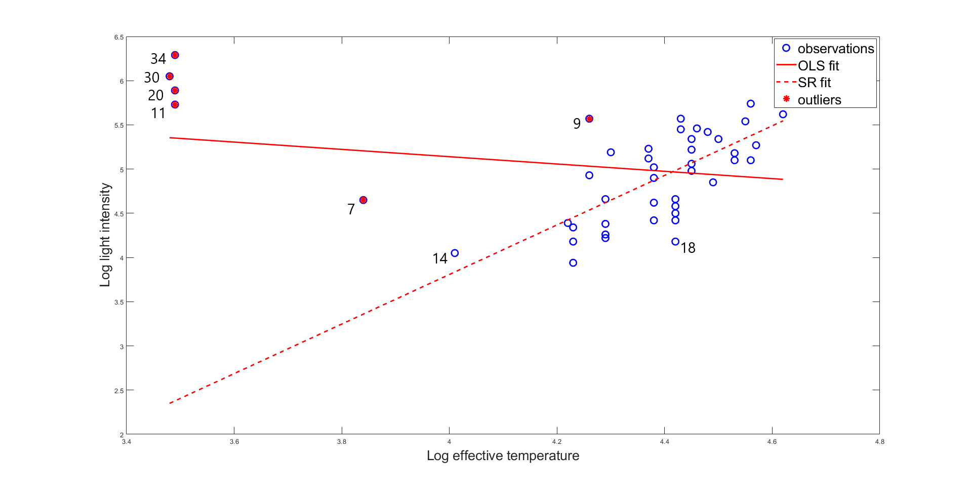
Figure 9: Star data-set with OLS and SR regression fit.

These giant stars actually represent a different population. They are bad leverage points because they influence OLS regression line due to the poor estimation of the parameters. Figure 9 shows how the four giant stars pull the OLS line towards them. Observations 7 and 9 are intermediate outliers. And finally, in the multivariate sense, observation 14 is often detected as outlier, but in the regression sense it is a good leverage point because it follows the same linear pattern than the bulk data. Robust regression fit made by the proposed method SR detected the giant stars 11, 20, 30, 34 and the intermediate outliers 7 and 9.

Table 13 summarizes all method’s estimation of the intercept and slope, and the outliers detected by the robust methods. Note that OLS estimates are completely changed, they have even different sign. SR and REWLSE correctly detect the regression outliers, method S detects the good leverage point, observation 14, as an outlier. LTS detects observation 18 as atypical when it is not. In Figure 9 it can be seen that observation 18 is an example of the swamping effect problem. On the other hand, MM approach only detects as outliers the giant stars (masking effect).

Table 13: Estimation of intercept and slope and detected outliers with star data.

Method	$\hat{\alpha}$	$\hat{\beta}$	Detected outliers
OLS	6.7935	-0.4133
SR	-7.4035	2.9028	7 9 11 20 30 34
LTS	-8.5001	3.0462	7 9 11 18 20 30 34
S	-10.5034	3.4994	7 9 11 14 20 30 34
REWLSE	-7.5001	3.0462	7 9 11 20 30 34
MM	-5.1234	2.2879	11 20 30 34

The $R^{2}$ values for the linear regression models fitted by each method are summarized in Table 14. OLS’s coefficient of determination is low, while that of the robust methods is high, except for MM approach which is lower than the rest.

Table 14: $R^{2}$ for each method with stars data-set.

Method	OLS	SR	LTS	S	REWLSE	MM
$R^{2}$	0.0443	0.7113	0.7006	0.7035	0.7095	0.5578

9.2 Hawkins-Bradu-Kass data

HBK data-set was artificially created by Hawkins et al. [1984] and it was also used in Leroy and Rousseeuw [1987], and many others. It contains $p=3$ explanatory variables and a response variable. The first 14 observations are leverage points: 1-10 of bad type and 11-14 of good type. Thus, only observations 1-10 are outliers in the regression sense. Table 15 shows the estimation by all methods for the three parameters, and it can be seen that OLS is highly influenced by the presence of these leverage points. Also, the parameter estimated by S method are different than that of the other robust approaches, and the reason for this is that all robust methods correctly detect the true outliers, except for method S, which also includes the good leverage points 11-14.

Table 15: Estimation of the parameters and detected outliers with HBK data.

Method	$\hat{\beta}_{0}$	$\hat{\beta}_{1}$	$\hat{\beta}_{2}$	$\hat{\beta}_{3}$	Detected outliers
OLS	-0.3875	0.2392	-0.3345	0.3833
SR	-0.1800	0.0836	0.0396	-0.0518	1 2 3 4 5 6 7 8 9 10
LTS	-0.1805	0.0814	0.0399	-0.0517	1 2 3 4 5 6 7 8 9 10
S	-0.0174	0.0957	0.0041	-0.1286	1 2 3 4 5 6 7 8 9 10 11 12 13 14
REWLSE	-0.1805	0.0814	0.0399	-0.0517	1 2 3 4 5 6 7 8 9 10
MM	-0.1913	0.0860	0.0412	-0.0541	1 2 3 4 5 6 7 8 9 10

The adjusted $R^{2}$ values are summarized in Table 16. Here, all robust methods, except S, have high and similar $R^{2}$.

Table 16: Adjusted $R^{2}$ for each method with HBK data-set.

Method	OLS	SR	LTS	S	REWLSE	MM
$R^{2}$	0.5850	0.9818	0.9816	0.9002	0.9817	0.9811

9.3 Living Environment Deprivation data

In Arribas-Bel et al. [2017], the authors studied the Living Environment Deprivation (LED) index. This measure allows to study quantitatively the concept of quality of the local environment, known also as urban quality of life, which is a qualitative concept. This is an essential matter for environmental research, citizens and politics. This kind of indices can be explained through remote sensing data, i.e. information collected without making physical contact, for example, from satellite technologies. The authors in Arribas-Bel et al. [2017] proposed to model the LED index of Liverpool (UK) based on four sets of explanatory variables extracted from a very high spatial resolution (VHR) image downloaded from Google Earth. The four groups are called: land cover (LC), spectral (SP), texture (TX) and structure features (ST). See Arribas-Bel et al. [2017] for more detailed description of the features. The authors first propose to explain the LED index with a linear combination of the four sets of variables. The linear regression model is the following:

$$LED=\alpha+\boldsymbol{\beta}LC+\boldsymbol{\gamma}SP+\boldsymbol{\delta}TX+\boldsymbol{\zeta}ST+\epsilon$$ (23)

There are $35$ explanatory variables, $\boldsymbol{\beta}$, $\boldsymbol{\gamma}$, $\boldsymbol{\delta}$ and $\boldsymbol{\zeta}$ are vectors, containing the parameters for each carrier, and $\epsilon$ is an error term assumed to be i.i.d. following a Gaussian distribution. The classical approach to estimate the regression parameters is using Ordinary Least Squares (OLS). The problem here is that the way of acquisition of the data, which is obtaing features from processing images from satellite technology, may imply the presence of atypical observations that could invalidate the results. Therefore, robust methodologies need to be used. On the other hand, the large number of variables derived from the Google Earth image, particularly those of spectral, texture and structure types, are substantially correlated (Figure 10).

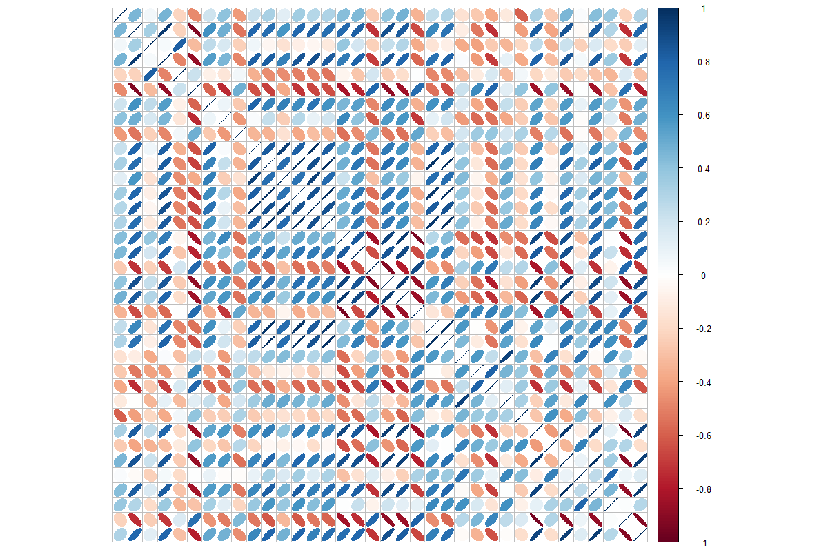
Figure 10: Correlation matrix for LED index data-set.

The multicollinearity issue violates another assumption for using OLS to estimate the parameters of the model. The authors propose to use a dimensionality-reduction step to preserve as much of the variation contained in the entire set of variables while eliminating collinearity. They performed a principal components analysis (pca) (Jolliffe [2011], Ballabio [2015]) on all the spectral, texture and structure variables, which makes a total of 27 variables, and after the analysis they propose to use only the first four components because they accounted for $90\%$ of the total variance. Other methods for data containing columns of uninformative variables in the regression problem have been proposed in the literature as well (Hoffmann et al. [2015], Li et al. [2018], Wang et al. [2019]). The four extracted components were used as regressors, together with the three land cover variables that prove most relevant: water, shadow, and vegetation. They came up with this result about the relevance by using another approach, but from machine learning area, which is the random forest (RF), since one of the main objectives of the paper was to study the potential of modern machine learning techniques: RF and gradient boost regressor (GBR), in the estimation of socioeconomic indices with remote-sensing data. Focusing on the classical OLS regression, the authors obtained that the third and fourth components were significant, as well as the proportion of an area occupied by water and vegetation.

We propose to study if the results can be improved by using robust regression methods. Let us apply the proposed SR approach and compare it with LTS, S, REWLSE and MM. The raw data, kindly provided by the authors was pre-processed the same way as they propose, by applying pca to the last 27 explanatory variables and join the first four components with the three land cover variables: water, shadow and vegetation, which makes a total of 7 explanatory variables. Table 17 shows the adjusted $R^{2}$ of the models estimated by each method.

Table 17: $R^{2}$ with (pca transformed) LED index data-set.

Method	OLS	SR	LTS	S	REWLSE	MM
$R^{2}$	0.5059	0.6716	0.6287	0.6031	0.5904	0.6166

Variables PC3, PC4, water and vegetation resulted significant in the model obtained by the methods. The percentage of variability explained by the robust methods shows the advantage of robust regression. The $R^{2}$ of SR is higher than that of the other approaches, although not as high as one would wish. The authors compare the results from OLS with the application of the two machine learning approaches. RF showed an $R^{2}=0.9354$ and GBR an $R^{2}=0.8320$. They were interested in finding the best possible model with the ability of capture as much proportion of the variation inherent in the data as possible. But the problem here is the drawback both machine learning methods have in terms of interpretability. Also, as the authors point out, RF and GBR suffer from the issue of overfitting. That is why they propose a cross validation (CV) study. It consisted on dividing the data in two groups, one to train the model, and the other one to test its predictive performance. The 5-fold CV was used and the procedure was repeated 250 times, to obtain the scores for the $R^{2}$, as in the paper. The scores for the MSE of the response are also saved. Table 18 shows the median cross-validated $R^{2}$ obtained by the authors for RF and GBR together with the one we obtained for method SR.

Table 18: Median cross-validated $R^{2}$ with (pca transformed) LED index data-set.

Method	SR	RF	GBR
$R^{2}$	0.6704	0.54	0.50

The results show that SR is more robust to overfitting since the $R^{2}$ is reduced slightly, while that of RF and GBR are significantly reduced. Between the three values, SR has the highest median cross-validated $R^{2}$. On the other hand, for method SR, the median absolute deviation from the data’s median (MAD) of these scores is 0.0145 which is low, meaning that the uncertainty is under control. Figure 11(a) shows the distribution of the cross-validated scores for the $R^{2}$ obtained with method SR and the median value in a dashed line.

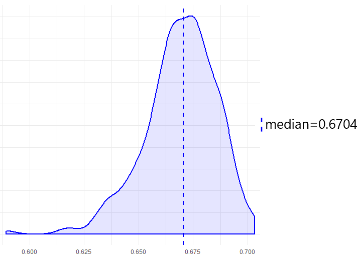
(a) Cross-validated $R^{2}$

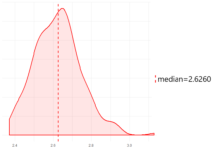
(b) Cross-validated MSE

Figure 11: CV scores and median values (dashed line), with pca.

Figure 11(b) shows the results for the MSE. The median of the cross-validated MSE is equal to 2.6260 and the MAD is 0.1199 which are also low values.

Since it was mentioned before, the same pca transformation the authors proposed for the data was made for this research. Now, we propose another transformation that improves the performance according to the results: sparse pca (spca) (Zou et al. [2006], Gajjar et al. [2017]), which has advantages in case of high correlated variables since it is a kind of variable selection transformation. The spca was made over the 27 variables of the three last groups and the first 10 components were selected since they account for $92.04\%$ of the total variance. These 10 components and the three most relevant land cover variables: water, shadow and vegetation were used to estimate the model.

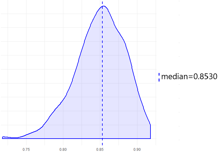
(a) Cross-validated $R^{2}$

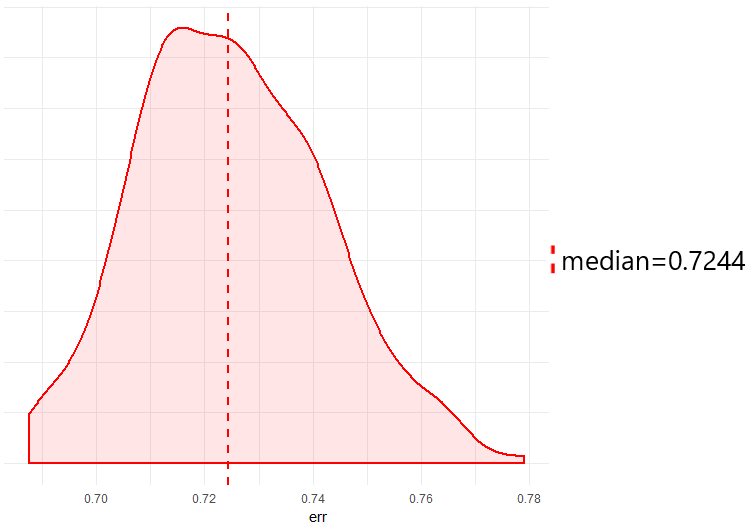
(b) Cross-validated MSE

Figure 12: CV measures and median values (dashed line), with spca.

Figure 12(a) shows the distribution of the cross-validated $R^{2}$ and the median value in a dashed line obtained with SR, which is 0.8530. The MAD of these scores increases to 0.0346 but it is still a low value. Figure 12(b) shows the distribution for the MSE. The median MSE reduces to 0.7244 and the MAD reduces to 0.0177. Table 19 shows that the median cross-validated $R^{2}$ is higher than that obtained with pca transformation but also higher than the obtained with both machine learning techniques, reported in Arribas-Bel et al. [2017].

Table 19: Median cross-validated $R^{2}$.

Method	SR spca	SR pca	RF	GBR
$R^{2}$	0.8530	0.6704	0.54	0.50

The uncertainty of the obtained $R^{2}$ is slightly higher with spca transformation, compared to that with the pca transformation. But Figure 13 shows that the distributions of the $R^{2}$ scores are quite separated, and the gain is obvious because of the increase in the median value.

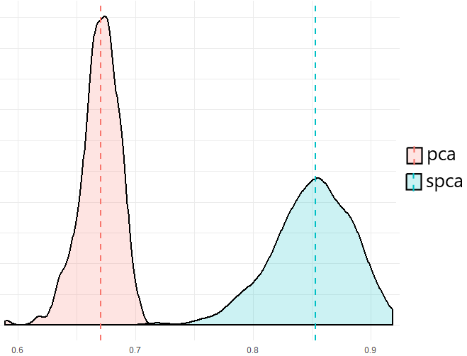
Figure 13: Cross-validated $R^{2}$ and median values (dashed line), for both pca and spca.

Finally, Table 20 contains the estimated coefficients, the p-values and the $R^{2}$ estimated by SR with spca transformation using the complete data-set, which is competitive with respect to the $R^{2}$ of RF and GBR reported in Arribas-Bel et al. [2017]. As the results point out, the same land cover variables as in the paper remained significant and with the same negative sign, meaning that larger proportions of water and vegetation are associated with smaller deprivation.

Table 20: Results for the model estimated by SR with spca transformation and the $R^{2}$ for RF and GBR.

	coefficient	p-value	RF	GBR
constant	0.27191	2.03E-05
water	-1.42641	2.00E-16
vegetation	-0.44513	2.00E-05
SPC2	-0.04409	4.51E-03
SPC3	0.13215	1.52E-06
SPC4	0.32566	1.03E-15
SPC5	-0.26745	2.35E-11
SPC7	-0.13735	2.24E-03
SPC8	0.19544	1.64E-03
$R^{2}$	0.86820		0.9354	0.8320

10 Conclusions

In the paper, the performance of the proposed SR approach is compared to the classical OLS and other existing robust regression methods. The robust alternatives in the literature have some drawbacks and their performance depend on decisions that, in case of real data, increase the difficulty of robustly estimate the regression parameters. On the other hand, not all available methods have a good behavior in case of large data-sets, high dimension, not all are scalable in terms of computational time, proven to be sufficiently resistant to the presence of outliers. The proposal in this paper is to use the notion of shrinkage in order to define robust estimators of location and scatter to estimate the regression parameters. The approach passes through a pair of weighting steps depending on robust Mahalanobis distances, which results in the shrinkage reweighted (SR) regression estimator. The advantages of using the shrinkage are shown in the simulation study and some conclusions can be noted. SR approach yielded competitive results compared to the alternative robust methods from the literature for the regression problem, even in high dimension, heavy-tailed distributed errors, large contamination or transformed data. Furthermore, SR is quite stable computationally since it involves contributions from all the observations instead of sub-sample iterations from the data. Finally, the results with the real data-set examples bear out with the conclusions from the simulation study. Specially with the LED index data where the SR approach provides an improvement of the cross-validated $R^{2}$ and MSE with respect to classical OLS and machine learning techniques RF and GBR, while maintaining the advantage of interpretability. It remains to be examined as future research if the proposal could be improved by using adjusted quantiles instead of the classical choices from the literature $q_{1}$ and $q_{2}$ from Equation 16, which are derived from the chi-squared distribution.

References

- Agulló et al. [2008] J. Agulló, C. Croux, and S. Van Aelst. The multivariate least-trimmed squares estimator. Journal of Multivariate Analysis, 99(3):311–338, 2008.
- Arribas-Bel et al. [2017] D. Arribas-Bel, J. E. Patino, and J. C. Duque. Remote sensing-based measurement of Living Environment Deprivation: Improving classical approaches with machine learning. PLOS ONE, 12(5):e0176684, 2017.
- Ballabio [2015] D. Ballabio. A MATLAB toolbox for Principal Component Analysis and unsupervised exploration of data structure. Chemometrics and Intelligent Laboratory Systems, 149:1–9, 2015.
- Cabana et al. [2019] E. Cabana, R. E. Lillo, and H. Laniado. Multivariate outlier detection based on a robust Mahalanobis distance with shrinkage estimators. 2019. URL http://arxiv.org/abs/1904.02596.
- Croux et al. [1994] C. Croux, P. J. Rousseeuw, and O. Hössjer. Generalized S-Estimators. Journal of the American Statistical Association, 89(428):1271, 1994.
- Croux et al. [2003] C. Croux, S. Van Aelst, and C. Dehon. Bounded influence regression using high breakdown scatter matrices. Annals of the Institute of Statistical Mathematics, 55(2):265–285, 2003.
- De Grève and Vanbeveren [1980] J. P. De Grève and D. Vanbeveren. Close binary systems before and after mass transfer: A comparison of observations and theory. Astrophysics and Space Science, 68(2):433–457, 1980.
- DeMiguel et al. [2013] V. DeMiguel, A. Martin-Utrera, and F. J. Nogales. Size matters: Optimal calibration of shrinkage estimators for portfolio selection. Journal of Banking & Finance, 37(8):3018–3034, 2013.
- Donoho and Huber [1983] D. L. Donoho and P. J. Huber. The notion of breakdown point. In A festschrift for Erich L. Lehmann, volume 157184. 1983.
- Edgeworth [1887] F. Y. Edgeworth. On observations relating to several quantities. Hermathena, 6:279–285, 1887.
- Falk [1997] M. Falk. On Mad and Comedians. Annals of the Institute of Statistical Mathematics, 49(4):615–644, 1997.
- Gajjar et al. [2017] S. Gajjar, M. Kulahci, and A. Palazoglu. Selection of non-zero loadings in sparse principal component analysis. Chemometrics and Intelligent Laboratory Systems, 162:160–171, 2017.
- Gervini and Yohai [2002] D. Gervini and V. J. Yohai. A class of robust and fully efficient regression estimators. The Annals of Statistics, 30(2):583–616, 2002.
- Hawkins and Olive [2002] D. M. Hawkins and D. J. Olive. Inconsistency of Resampling Algorithms for High-Breakdown Regression Estimators and a New Algorithm. Journal of the American Statistical Association, 97(457):136–148, 2002.
- Hawkins et al. [1984] D. M. Hawkins, D. Bradu, and G. V. Kass. Location of Several Outliers in Multiple-Regression Data Using Elemental Sets. Technometrics, 26(3):197, 1984.
- Hoffmann et al. [2015] I. Hoffmann, S. Serneels, P. Filzmoser, and C. Croux. Sparse partial robust M regression. Chemometrics and Intelligent Laboratory Systems, 149:50–59, 2015.
- Huber [1964] P. J. Huber. Robust Estimation of a Location Parameter. The Annals of Mathematical Statistics, 35(1):73–101, 1964.
- Huber [1973] P. J. Huber. Robust Regression: Asymptotics, Conjectures and Monte Carlo. The Annals of Statistics, 1(5):799–821, 1973.
- Huber [1981] P. J. Huber. Robust statistics. New York John Wiley and Sons, 1981.
- Humphreys [1978] R. M. Humphreys. Studies of luminous stars in nearby galaxies. I. Supergiants and O stars in the Milky Way. The Astrophysical Journal Supplement Series, 38:309, 1978.
- James and Stein [1992] W. James and C. Stein. Estimation with Quadratic Loss. In Breakthroughs in statistics, pages 443–460. Springer, New York, NY, 1992.
- Jolliffe [2011] I. Jolliffe. Principal Component Analysis. In International Encyclopedia of Statistical Science, pages 1094–1096. Springer Berlin Heidelberg, Berlin, Heidelberg, 2011.
- Ledoit and Wolf [2003a] O. Ledoit and M. Wolf. Improved estimation of the covariance matrix of stock returns with an application to portfolio selection. Journal of Empirical Finance, 10(5):603–621, 2003a.
- Ledoit and Wolf [2004] O. Ledoit and M. Wolf. A well-conditioned estimator for large-dimensional covariance matrices. Journal of Multivariate Analysis, 88(2):365–411, 2004.
- Ledoit and Wolf [2003b] O. Ledoit and M. N. Wolf. Honey, I Shrunk the Sample Covariance Matrix. UPF Economics and Business Working Paper No. 691, 2003b.
- Leroy and Rousseeuw [1987] A. M. Leroy and P. J. Rousseeuw. Robust regression and outlier detection. 1987.
- Li et al. [2018] H.-D. Li, Q.-S. Xu, and Y.-Z. Liang. libPLS: An integrated library for partial least squares regression and linear discriminant analysis. Chemometrics and Intelligent Laboratory Systems, 176:34–43, 2018.
- Lopuhaa and Rousseeuw [1991] H. P. Lopuhaa and P. J. Rousseeuw. Breakdown points of affine equivariant estimators of multivariate location and covariance matrices. The Annals of Statistics, 19(1):229–248, 1991.