Deep Blind Video Decaptioning by Temporal Aggregation and Recurrence

Abstract

Blind video decaptioning is a problem of automatically removing text overlays and inpainting the occluded parts in videos without any input masks. While recent deep learning based inpainting methods deal with a single image and mostly assume that the positions of the corrupted pixels are known, we aim at automatic text removal in video sequences without mask information. In this paper, we propose a simple yet effective framework for fast blind video decaptioning. We construct an encoder-decoder model, where the encoder takes multiple source frames that can provide visible pixels revealed from the scene dynamics. These hints are aggregated and fed into the decoder. We apply a residual connection from the input frame to the decoder output to enforce our network to focus on the corrupted regions only. Our proposed model was ranked in the first place in the ECCV Chalearn 2018 LAP Inpainting Competition Track2: Video decaptioning. In addition, we further improve this strong model by applying a recurrent feedback. The recurrent feedback not only enforces temporal coherence but also provides strong clues on where the corrupted pixels are. Both qualitative and quantitative experiments demonstrate that our full model produces accurate and temporally consistent video results in real time (50+ fps).

1 Introduction

Dealing with missing or corrupted data is a crucial step before consuming visual contents. In many applications in image/video processing, such incompleteness degrades the visual perception for both human and machines. To overcome this limitation, recent approaches have focused on solving denoising [30], restoration [20], super-resolution [6], and inpainting [22]. In this paper, we focus on video decaptioning, one of the video inpainting tasks where the solution can be directly applicable to real-world video restoration scenarios.

In the context of media and video data from various languages, there are frequently text captions or encrusted commercials. These text overlays reduce visual attention and occlude parts of frames. Removing the text overlays and inpainting the occluded parts require the understanding of the spatio-temporal context in videos. However, processing a video sequence requires high memory footprint and time complexity due to the additional time dimension.

Figure 1: Overview of our blind video decaptioning network. (BVDNet) We propose a hybrid encoder-decoder model, where the aggregation encoder stream takes multiple input frames and the decoder reconstructs the middle frame. The temporal-pooling skip connections carry low-level information. By a residual learning algorithm, our model directly learns to recover the corrupted pixels in the input. The output is then fed into a feedback connection for a recurrent learning to the next time step.

A straightforward way to perform video decaptioning is to recover a video frame-by-frame. However, it loses a great advantage coming from the video dynamics. In many subtitled videos, the occluded parts in a frame are often revealed in its neighboring frames if the object moves out of the text overlay or the subtitles disappear (e.g. Fig. 4-a). Also, since dealing with a single frame does not consider any temporal consistency, the consecutive frames in the recovered video are not likely to be connected naturally. The video captions which disappear or change very suddenly and independently to the visual semantics make it more challenging to maintain the temporal stability. Post-processing with off-the-shelf techniques like blind video temporal consistency [17] is also not applicable, since they require reference video sequences with dense optical flows which are not reliable in our case due to the corrupted regions.

Another challenge in automatic text removal is that the binary indicator (i.e. inpainting mask) for the corrupted pixels is not given in advance. In contrast, most existing inpainting methods [22, 31, 34] usually assume that the binary pixel mask is available and use different image priors based on it. We cannot directly adopt their scenarios because annotating (or creating) such pixel masks for every frame in videos is impractical and limits the system’s autonomy. Furthermore, many video subtitles include semi-transparent shadows (as in Fig. 1, Fig. 4-a, b) where it is ambiguous to label the pixels in binary. These regions should not be considered as solid occlusions, because of the underlying information.

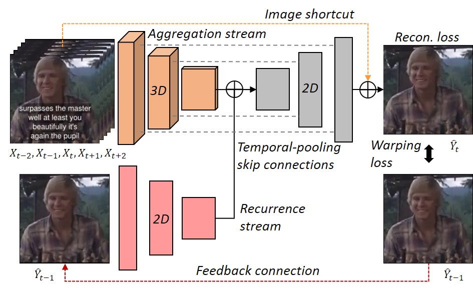
To overcome the aforementioned challenges in blind video decaptioning, we propose a simple yet effective encoder-decoder model (see Fig. 1), where the encoder aggregates spatio-temporal context from neighboring source frames and the decoder reconstructs the target frame. We apply a residual learning algorithm where our network is encouraged to touch only the corrupted pixels. We further introduce a recurrent feedback connection, so that the generation of the target frame is based on the previously generated frame. Since the features from the neighbor frames and the previous output are largely dissimilar on the corrupted regions, it helps our network to better detect corrupted pixels and boosts the performance. We train our model with the gradient reconstruction loss and the structural similarity loss in conjunction with the conventional L1 loss. We validate the contribution of our design components through experiments. To our best knowledge, this is the first attempt to apply deep learning to the blind video inpainting application.

Our contribution can be summarized as follows:

• Unlike most of the existing methods for image/video inpainting, the proposed approach aggregates neighboring spatio-temporal features in the encoder and recovers a decaptioned frame in the decoder without requiring the inpainting masks.

• We design an effective and robust loss function for video decaptioning and empirically validate the usefulness of the loss terms with our architectural design by extensive ablation study.

• Our model outperforms other competing methods and runs in real time (50+ fps). We took the first place in the ECCV Chalearn 2018 LAP Video Decaptioning Challenge.

• We further improve our model by introducing a recurrence mechanism and boost the performance even more in terms of both visual quality and temporal coherency.

2 Related Work

2.1 Image Inpainting

Approaches of traditional image inpainting make use of the image-level features to diffuse the texture from the surrounding context to the missing hole [1, 3]. These methods can only tackle small holes and would lead to noise patterns and artifacts for large holes. Later works using patch-based methods could optimize the inpainting performance by searching the best matching patches [7, 2]. However, while these methods could provide plausible texture generation in the hole, they are not aware of the high-level semantics of the image and cannot make reasonable inference for object completion and structure prediction.

Recently, many image inpainting models based on Convolutional Neural Networks (CNNs) have been proposed [22, 31, 32, 13, 34, 19, 33]. These approaches directly infer pixel values inside holes in an end-to-end fashion. Thanks to their ability to learn adaptive image features of various semantics, they can synthesize pixels that are more visually plausible. Pathak et al. [22] introduced Context Encoder that enabled to fill large masks using a CNN model. They proposed to use Generative Adversarial Networks (GAN) [9] to avoid the blurring artifacts. Iizuka et al. [13] proposed a fully convolutional network with both global and local discriminators to obtain semantically and locally coherent image inpainting results. This method, however, heavily relies on a post-processing step; Poisson image blending. Yu et al. [34] proposed a coarse-to-fine model by stacking two generative networks, ensuring the color and texture consistency of generated regions with surroundings. Moreover, in order to capture long-range spatial dependencies, a contextual attention module is integrated into the networks. However, this model does not generalize well on irregular masks because it is mainly trained on large rectangular masks. To better handle free-form masks, partial convolution [19] and gated convolution [33] are proposed where the convolution weights are masked or re-weighted respectively to utilize valid pixels only.

Figure 2: Multiple time steps of our BVDNet framework. The image shortcuts, input to the recurrence stream, and input to the aggregation stream are represented by orange, red, and black arrows, respectively. We mirror-pad at initial input boundary (e.g.$t$=1,2) as illustrated in stripe pattern. Our method processes frames sequentially in a sliding window manner and produces the video results in real time.

2.2 Video Inpainting

Approaches for video inpainting can be categorized into object-based and patch-based methods. Object-based approahces [5, 16, 18] segment a video into moving foreground objects and background that is either still or exhibits smooth motion. The moving objects are, in general, copied into the holes as smoothly as possible, whereas the background is inpainted using image inpainting methods. However, such approaches work well only when the objects’ motion shows strict periodicity.

The patch-based method [23] copied and pasted small video patches into the holes. Patwardhan et al. [24] further improved this approach so that moving cameras could be dealt with. Granados et al. [10] proposed a semi-automatic algorithm which optimizes the spatio-temporal shift map [25]. However, manual tracking of moving objects is required to reduce a large search space and high computational complexity. Further, Wexler et al. [29] proposed an iterative method to solve a global optimization method. However, these methods rely on the inpainting masks for each frame and lack high-level semantic understanding. Newson et al. [21] extend this by developing a 3D version of PatchMatch [2]. Huang et al. [12] propose to use additional optical flow term by modifying the energy term of  [29] for temporally coherent predictions in results.

Our work takes an important next step beyond the aforementioned prior works in that we address a blind video inpainting task using a deep CNN model. We propose a 3D encoder-2D decoder model that can effectively learn spatio-temporal features to recover clear frames in a data-driven manner. Our predicted frames are visually natural and temporally smooth without any post-processing step. Thanks to our light-weight design, the overall process performs in real-time (50+ fps).

3 Proposed Method

Video decaptioning aims to estimate original frames {$\hat{Y}$} from the subtitled, noised frames {$X$}. The recovered region should either be as accurate as in the GT frames {$Y$} or seamlessly merged into the surrounding pixels. Our strategy is to collect hints from the multiple neighboring (source) frames and recover a target frame. This is to leverage the scene dynamics in a video where the occluded parts are often revealed in the lagging or leading frames as the objects move or the subtitles change. We also propose to use a recurrent feedback connection as an additional source stream. This helps our network to reduce temporal flickering and to automatically detect the corrupted regions.

3.1 Residual Learning

Directly estimating all pixels in a frame may needlessly touch uncorrupted pixels. To deal with the absence of the pixel indicators (inpainting masks), we train our model by a residual learning algorithm. Specifically, the final output is yielded by summing the input center frame {$X_{t}$} and the predicted residual image {$R_{t}$} in a pixel-wise manner. This encourages our network to explicitly focus on the corrupted pixels only, and also prevent the global tone distortion.

Formally, with the proposed decaption model $f$, we model the video captioning problem as

$$\hat{Y_{t}}=f(X_{t-N:t+N},\hat{Y}_{t-1})+X_{t},$$ (1)

where $t$ denotes a frame index and $N$ is a temporal radius.

3.2 Network Design

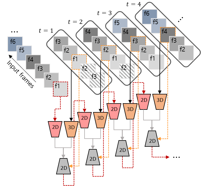
The overall decaptioning algorithm is illustrated in Fig. 1. Our core design is a hybrid encoder-decoder model, where the encoder consists of two sub-networks: 3D CNN and 2D CNN. The decoder follows a normal 2D CNN design as in other image generation networks. The network is designed to be fully convolutional, which can handle arbitrary size input. The final output video is obtained by applying $f$ in an auto-regressive manner as in Fig. 2.

Two-stream encoder.  Our strategy is to collect potential hints from multiple source frames that can provide visible pixels revealed from the scene dynamics. Also, we enforce the generation of the target frame to be consistent with the previous generation. We construct a two-stream hybrid encoder where each source stream is trained to achieve our objectives. The first encoder stream consists in 3D convolutions which can directly capture spatio-temporal features from the neighboring frames. This can help in understanding the short-term video-level context which is required to recover the target frame. The input tensor shape is $H\times W\times T\times C$, where $H$,$W$ and $C$ are the height, width and channels of the input frame $\{X\}$, and $T=2N+1$. We use $N=2$ in our network ($T=5$). Here, the goal is to remove text overlays in the center input frame (3th out of 5). The temporal dimension gradually reduces into 1 passing through the 3D convolution layers in this stream.

The second stream is a 2D CNN which takes the previously generated frame, of size $H\times W\times 1\times C$, as input. This stream provides a reference for the current generation to be temporally coherent with. Moreover, the encoded feature is combined with the temporally-pooled one-frame feature from the first stream by element-wise summation. Since the features from the two streams are comparatively different on the corrupted regions, the combined hybrid feature map implicitly encodes the knowledge on where to attend.

Bottleneck and temporal-pooling skip connections.

The encoder is followed by bottleneck layers that consist of several dilated convolutions, as suggested in [13]. The large receptive field size helps to capture wide spatial context which supports the recovery of the corrupted pixels. The following is a 2D CNN decoder which is symmetric to the 2D encoder stream.

We apply skip connections only between the 3D encoder stream and the decoder. Each skip connections pass through a 3D convolution layer that pools the temporal dimension into one frame, so that the feature map can be directly concatenated with the decoder features of equal dimension. Despite the concern raised by Yu et al. [33] that the skip connections carry almost zero features on the corrupted regions, our temporal-pooling skip connections are immune to this problem since they can adaptively aggregate low-level features that are complementary to the occluded points in the center frame.

Our full network is trained to generate the residual frame {$R_{t}$}, which is added with the input center frame {$X_{t}$} to produce the final output {$\hat{Y_{t}}$}.

3.3 Frame Sampling

As we mentioned earlier, our task can greatly benefit from the video dynamics. If the scene moves or the subtitles disappear in the neighboring frames, the occluded parts will be revealed, which provides critical clues to the underlying content. To maximize this gain, we attempt to find the optimal frame sampling interval for our model. With the minimum interval of 1, the input frames will contain non-significant dynamics. If we jump with large stride, on the other hand, irrelevant new scenes will be included. We empirically find that the stride of 3 performs the best in our preliminary experiment. Since we use $T=5$, our model has about 15 frame-term view range.

3.4 Loss Functions

We train the sequential video decaptioning model $f$ by solving the following objective function,

$$\min_{f}\left(\lambda_{R}\mathcal{L}_{R}(f)+\lambda_{T}\mathcal{L}_{T}(f)\right),$$ (2)

where $\mathcal{L}_{R}$ is an image reconstruction loss, and $\mathcal{L}_{T}$ is a temporal consistency loss. $\lambda_{R}$ and $\lambda_{T}$ denote to the weighting coefficients which are set to 1 and 2 throughout the experiments.

To address image reconstruction, a simple way is to minimize the L1 loss following the previous studies [19, 34]. For the structural details, We apply the SSIM loss [28] with a small patch window according to the setting of the competition evaluation metric. Inspired by [8], we also use a first-order matching term, which compares image gradients of the prediction with the ground truth, and encourages the prediction to have not only close-by values but also similar local structure. To this end, the image reconstruction loss $\mathcal{L}_{R}$ includes three terms as

$$\pazocal{L}_{1}=\left\|\hat{Y_{t}}-Y_{t}\right\|_{1},$$ (3)

$$\pazocal{L}_{SSIM}=(\frac{{(2\mu_{\hat{Y_{t}}}\mu_{Y_{t}}+c_{1})(2\sigma_{\hat{Y_{t}}{Y_{t}}}+c_{2})}}{{(\mu_{\hat{Y_{t}}}^{2}+\mu_{Y_{t}}^{2}+c_{1})(\sigma_{\hat{Y_{t}}}^{2}+\sigma_{Y_{t}}^{2}+c_{2})}}),$$ (4)

$$\pazocal{L}_{grad.}=\left\|\nabla_{W}(\hat{Y_{t}}-Y_{t})\right\|_{1}+\left\|\nabla_{H}(\hat{Y_{t}}-Y_{t})\right\|_{1},$$ (5)

$$\pazocal{L}_{R}=\pazocal{L}_{1}+\pazocal{L}_{SSIM}+\pazocal{L}_{grad.},$$ (6)

where $\hat{Y_{t}},Y_{t}$ denote the predicted and target groundtruth frames respectively. $\mu,\sigma$ denote the average, variance. $c_{1},c_{2}$ denote two stabilization constants which are respectively set to $0.01^{2},0.03^{2}$. $\nabla_{W},\nabla_{H}$ are the image gradients along the horizontal and vertical axis.

With the recurrence (second) stream in the encoder, we optimize our model with additional temporal warping loss which is widely used in video generation works [17, 27, 11]. The temporal consistency loss $\mathcal{L}_{T}$ is defined as

$$\pazocal{L}_{T}=\sum\limits_{t=1}^{T-1}M_{t-1}^{t}\left\|\hat{Y_{t}}-\phi({Y}_{t-1})\right\|_{1},$$ (7)

where $M$ represents the binary occlusion mask and $\phi$ denotes the flow warping operation. We use optical flow between consecutive target frames obtained by FlowNet2 [14], to compute our temporal loss. For the training, we set the number of recurrences to 5 $(T=5)$.

	Architecture			Losses			Recurrence	Evaluation Metric
Exp	3D-3D	2D-2D	3D-2D	L1	grad. L1	SSIM	Enc. Stream	MSE	PSNR	DSSIM
1	✓			✓				0.0031	28.4590	0.0652
2		✓		✓				0.0012	33.6803	0.0279
3			✓	✓				0.0011	34.1029	0.0261
4			✓	✓	✓			0.0010	34.2251	0.0276
5			✓	✓	✓	✓		0.0010	34.6544	0.0225
6 (Our full model)			✓	✓	✓	✓	✓	0.0010	34.7055	0.0222

Table 1: The ablation studies on architectural design, loss functions, and recurrence stream. We evaluate on ChaLearn 2018 LAP Inpainting Track2 validation set.

4 Implementation

Dataset.  We used the ECCV Chalearn 2018 LAP Video Decaptioning Challenge dataset for training, validation, and testing. It is a large dataset of 5 seconds (125 frames) MP4 video clips in $128\times 128$ pixel RGB frames, containing both encrusted subtitles ({$X$}) and without subtitles ({$Y$}). The dataset contains a wide variety of captions with different colors, size, positions, and shadows. The training and validation set consist in 70K and 5K sample pairs of input and ground truth video clips, respectively. The testing set consists of 5K input video clips without ground truth. We convert every video clip into PNG images in our experiments.

Training.  We adopt horizontal flipping and color jittering for data augmentation. We train our model for 200 epochs with a batch size of 128. Adam optimizer is used with $\beta$ = (0.9, 0.999) and a learning rate of 0.001. The training takes 3 days on two NVIDIA GTX 1080 Ti GPUs. For the competition, we train our model without the recurrence stream in the encoder and the warping loss.

Testing.  For the pixels where the absolute difference between the input middle frame $\{X_{t}\}$ and the prediction $\{\hat{Y_{t}}\}$ is less than 0.01 in $[0,1]$ scale, we copy the values from the input frame. Finally, we convert PNG files back to MP4 videos.

Evaluation Metric.  To evaluate the quality of the reconstruction, the mean square error (MSE), the peak signal-to-noise ratio (PSNR), and the structural dissimilarity (DSSIM – i.e. (1-SSIM)/2) are used.

(a) input	(b) L1	(c) L1 + grad.L1	(d) L1+grad.L1+SSIM	(e) target (groundtruth)

Figure 3: The impact of each loss terms. (a) An input center frame. (b-d) The reconstructed frames with: (b) L1 loss, (c) L1 + gradient L1 loss, and (d) L1 + gradient L1 + SSIM loss. (e) Ground truth frame. Best viewed when zoomed-in.

(a)	(b)

Figure 4: The impact of recurrence on temporal consistency. For each sample, we visualize four consecutive input frames in the top row. In the bottom rows are the zoomed-in views of our results without recurrence (2nd row), with recurrence (3rd row), and the ground truth frames (4th row). Without the recurrence, the change in the subtitles leads to temporally flickering artifacts (a)

	Ours	+ GAN loss	- Skip
MSE	0.0010	0.0015	0.0010
PSNR	34.7055	31.2257	34.3892
DSSIM	0.0222	0.0384	0.0233

Table 2: The ablation studies on additional GAN loss and without residual learning. We evaluate on ChaLearn 2018 LAP Inpainting Track2 validation set.

	Value	MSE	PSNR	DSSIM
	3	0.0011	33.7895	0.0247
Number	5	0.0010	34.7055	0.0222
of frames	7	0.0010	34.5063	0.0229
	9	0.0010	34.6260	0.0226

Table 3: The ablation studies on the hyperparamter: number of input frames. We evaluate on ChaLearn 2018 LAP Inpainting Track2 validation set.

Encoder version	Temporal Errors
without recurrence (Ours-Exp 5)	0.00117
with recurrence (Ours-Exp 6)	0.00090

Table 4: Temporal errors (warping errors) of our full model with and without temporal consistency constraints. We evaluate on 500 clips of ChaLearn 2018 LAP Inpainting Track2 validation set.

5 Experimental Results

5.1 Ablation Study

In order to evaluate the effectiveness of different components of the proposed BVDNet, we conduct ablation studies using the publicly released validation set.

The impact of 3D encoder stream. One of our core design choices is to use a 3D CNN encoder stream in conjunction with a following 2D decoder. To validate the effectiveness of this design, we construct two naive baselines to compare with: a 3D encoder-3D decoder and a 2D encoder-2D decoder models. We note that all models in this experiment contain a single-stream encoder without the recurrence stream encoder for a clearer comparison. We construct all the models with a comparable number of parameters. As shown in Exp 1, 2, and 3 in Table 1, our 3D-2D model shows the best performances in all three metrics. This implies that spatio-temporal feature extraction from the neighboring frames indeed helps our target task, providing our model with a distinct advantage over the frame-by-frame competitor. On the other hand, it is empirically shown that adopting heavy 3D-3D operations does more harm than good. This implies that making use of the neighboring frames does not always work, rather the careful architectural design is required.

The impact of loss functions.  We test our loss functions both quantitatively and qualitatively. First, we remove each loss terms gradually from our full loss function. Again, we use models with the single-stream encoder, and thus the temporal warping loss is not considered in this experiment. As shown in Exp 3, 4, and 5 in Table 1, the best scores are obtained in all metrics when all L1, gradient L1, and SSIM losses are used together.

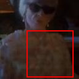
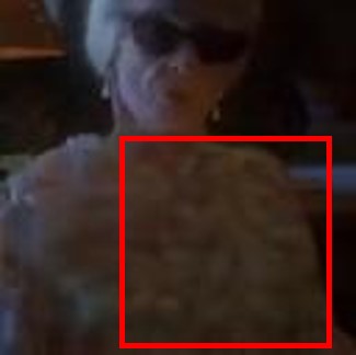
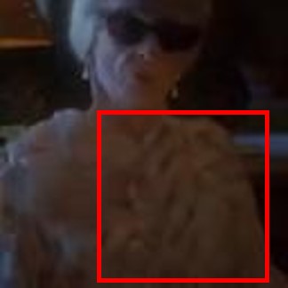
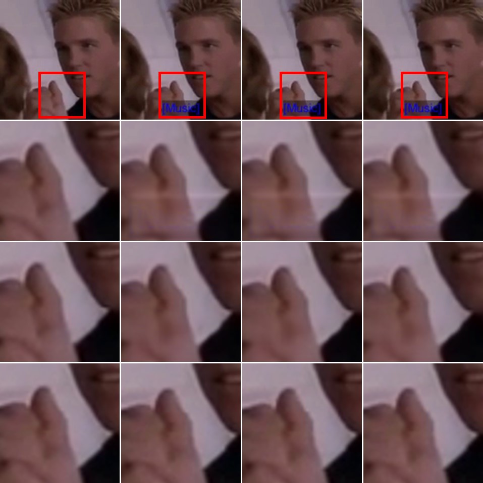
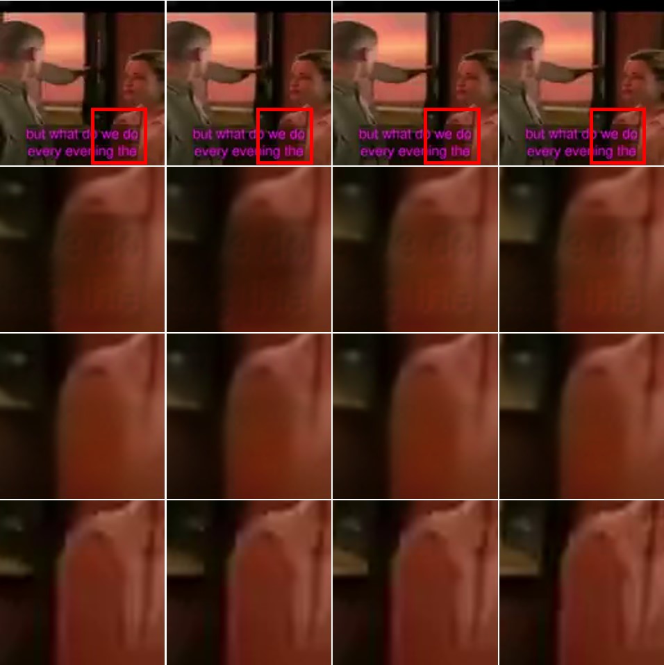
We also provide qualitative analysis as shown in Fig. 3. The model trained with the L1 loss alone produces relatively blurry outputs. We alleviated this problem by adding the gradient L1 loss and the SSIM loss. We attempt to use the adversarial loss, but it tends to decrease the performance on the evaluation metrics (see  Table 2). We observe that the gradient L1 and SSIM losses together help recover finer structures (texture and edge) and achieve better evaluation scores as well. In short, the L1 loss plays a role of capturing the overall structure of the corrupted region. The gradient L1 loss and the SSIM loss reduce the artifacts, encouraging the preservation of the local structures.

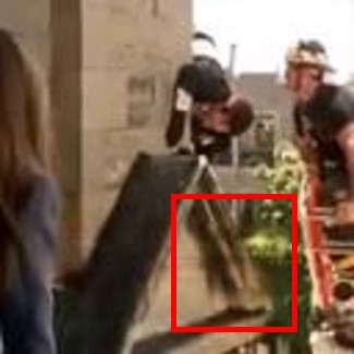
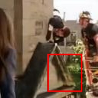
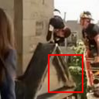
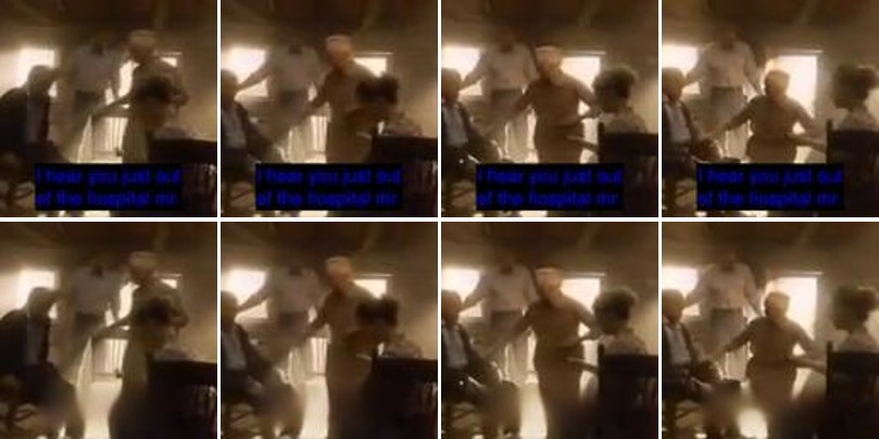
The impact of the recurrence encoder stream.  We investigate the effectiveness of our recurrence stream in the encoder, together with the temporal warping loss. We evaluate both frame-level image quality and temporal consistency. As shown in Exp 5 and 6 in Table 1, the recurrence stream improves the visual quality of the video results. In addition, we quantitatively compare the temporal consistency of our models with and without the recurrence stream. We measure the temporal error over a video sequence, which is the average pixel-wise Euclidean color difference between consecutive frames. We use FlowNet2 [14] to obtain pseudo-groundtruth optical flows as in the training. Table 4 shows that the temporal error is significantly reduced by having the recurrence stream in the encoder. Our approach does not sacrifice either visual quality and temporal stability. This is also shown qualitatively in Fig. 4. These results imply that the recurrence stream helps our model to better detect and inpaint the corrupted regions automatically, in a temporally coherent manner.

Adding GAN loss.  The adversarial training encourages the decaptioning results to move towards the natural image manifold. We test the effect of the adversarial training by adding the GAN loss on top of our full loss function. We use $8\times 8$ PatchGAN [15] as our discriminator network that aims to classify whether $8\times 8$ overlapping image patches are real or fake. However, we observe no visible qualitative improvement and the quantitative performance slightly dropped (Table 2), which is consistent with the results in [26].

Removing residual image shortcut.  We investigate the importance of the residual learning. If we remove the skip connection from the input center frame to the decoder output, the network should predict the uncorrupted output without referencing the input pixels. As shown in the  Table 2, adopting the residual learning scheme shows better performances, demonstrating that devoting to the pixels to be recovered is more effective for video decaptioning.

Number of input frames.  In Table 3, we perform an experiment to determine the hyperparameter $T$ for our model, which is the number of input frames. The number of input frames directly relates to the size of input batches, which enables to control the amount of temporal information to be considered at once. Table 3 shows the comparison results with four different input frame values. We observe that the performance tends to be good with larger input frames in general, while the value of 5 gives the best results. This indicates that having proper temporal view range is crucial for video decaptioning.

5.2 Model Inference Time

Our full model has a total of 23 layers and 10.5M parameters. Our model is implemented on Pytorch v0.3, CUDNN v6.0, CUDA v8.0, and run on the hardware with Intel(R) Xeon(R) (2.10GHz) CPU and NVIDIA GTX 1080 Ti GPU. The model runs at 62.5 fps on a GPU for frames of resolution 128 $\times$ 128 px.

	MSE	PSNR	DSSIM
stephane	0.0022	30.1856	0.0613
hcilab	0.0012	33.0228	0.0424
anubhap93	0.0012	32.0021	0.0499
arnavkj95	0.0012	32.1713	0.0482
Ours	0.0011	33.3527	0.0404

Table 5: Final performances of the top entries in the ECCV ChaLearn 2018 LAP Inpainting Challenge Track2 test phase. We note that stephane’s is the baseline from the organizers [4].

5.3 Final Challenge Results

Quantitative results. Table 5 summarizes the top entries from the leaderboard of ECCV ChaLearn 2018 Inpainting Challenge Track2. We participated with our model without the recurrence stream and achieved the first place on the final test phase. The source code and factsheet are publicly available at http://chalearnlap.cvc.uab.es/challenge/26/track/31/result/fact-sheet/237/.

Our full model is even stronger on the validation set as shown in Table 4, but we cannot evaluate the full model on the testing set because the test server is closed.

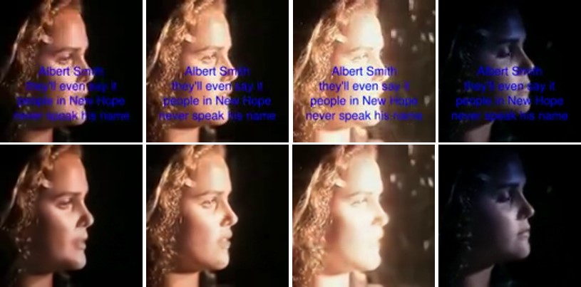
Qualitative results.  We visualize the learned feature maps of our full model in Fig. 5. We observe a hierarchical attention where the 3D encoder layers captures low-level features such as background texture features along time axis, and the 2D decoder layers then gradually attend to the exact corrupted region to recover the original content.

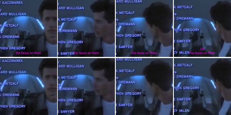
Fig. 6 shows examples of our decaptioning results. Our full model successfully recovers the video frames with smooth temporal transition even when there are active object movements as in Fig. 6-(a). Also, fine details and textures are well reconstructed even when heavy illumination change exists as in Fig. 6-(b). Even when there are non-caption texts in the video, e.g. Fig. 6-(c), our algorithm is able to separate between the text overlays and texts coming from the video. However, the results are relatively blurry when the input frames have a solid shadow which makes complete occlusions, as in Fig. 6-(d). This is probably due to the lack of samples with such solid shadows in the given training set.

(a) input	(b) enc-64

(c) enc-32	(d) dec-32	(e) dec-64	(f) output

Figure 5: Visualization of learned feature activation. For the visualization, we average each feature maps along the channel axis, perform zero-one normalization, and up-sample to $128\times 128$ px. The numbers in the labels denote spatial resolution of the feature maps. We observe hierarchical attention operations across the network. In the early encoder layers (b, c), low-level features such as background textures ( e.g.around the subtitles) are aggregated along the time dimension. The latter decoder layers (d, e) then gradually focus on the exact target regions ( e.g.on the subtitles) which require high-level semantics to be synthesized.

(a)	(b)
(c)	(d)

Figure 6: Qualitative decaptioning results. For each example, the top rows are the input sequences and the bottom rows are the decaptioning results using our full model. For visualization, we determine the time interval between the frames to be 0.1 seconds. Our model performs well on various types of subtitles with complex background variations and also is able to separate the non-caption texts in a video.

6 Conclusion

In this paper, we propose a deep network model for fast blind video decaptioning that learns to remove text overlays in videos. Our model collects hints from not only the current frame but also the future and the past neighboring frames. In addition, it generates each frame conditionally to the previous output frame for the temporal consistency preserving. We design an encoder-decoder model, where the hybrid encoder consists of a 3D CNN stream and a recurrent feedback stream. The spatio-temporal features from these multiple source streams are extracted and fed into the image-based decoder. The skip connections from the 3D encoder stream aggregate low-level features along the time axis, so that they can complement the corrupted feature points. Based on our residual learning algorithm and robust loss function design, the proposed framework is ranked in the first place in the ECCV Chalearn 2018 LAP Inpainting Track2 - Video decaptioning Challenge. We hope our proposed model will become an important basic architecture for solving real-world video restoration tasks.

Acknowledgements

Dahun Kim was partially supported by Global Ph.D. Fellowship Program through the National Research Foundation of Korea (NRF) funded by the Ministry of Education (NRF-2018H1A2A1062075).

References

- [1] C. Ballester, M. Bertalmio, V. Caselles, G. Sapiro, and J. Verdera. Filling-in by joint interpolation of vector fields and gray levels. IEEE transactions on image processing, 10(8):1200–1211, 2001.
- [2] C. Barnes, E. Shechtman, A. Finkelstein, and D. B. Goldman. Patchmatch: A randomized correspondence algorithm for structural image editing. ACM Transactions on Graphics (ToG), 28(3):24, 2009.
- [3] M. Bertalmio, G. Sapiro, V. Caselles, and C. Ballester. Image inpainting. In Proceedings of the 27th annual conference on Computer graphics and interactive techniques, pages 417–424, 2000.
- [4] Chalearn-Baseline. Eccv 2018 chalearn challenge track2 official website. http://chalearnlap.cvc.uab.es/challenge/26/track/31/baseline/, 2018.
- [5] S.-C. S. Cheung, J. Zhao, and M. V. Venkatesh. Efficient object-based video inpainting. In Image Processing, 2006 IEEE International Conference on, pages 705–708. IEEE, 2006.
- [6] C. Dong, C. C. Loy, K. He, and X. Tang. Image super-resolution using deep convolutional networks. IEEE transactions on pattern analysis and machine intelligence, 38(2):295–307, 2016.
- [7] A. A. Efros and T. K. Leung. Texture synthesis by non-parametric sampling. In iccv, page 1033. IEEE, 1999.
- [8] D. Eigen and R. Fergus. Predicting depth, surface normals and semantic labels with a common multi-scale convolutional architecture. In Proceedings of the IEEE International Conference on Computer Vision, pages 2650–2658, 2015.
- [9] I. Goodfellow, J. Pouget-Abadie, M. Mirza, B. Xu, D. Warde-Farley, S. Ozair, A. Courville, and Y. Bengio. Generative adversarial nets. In Advances in neural information processing systems, pages 2672–2680, 2014.
- [10] M. Granados, J. Tompkin, K. Kim, O. Grau, J. Kautz, and C. Theobalt. How not to be seen—object removal from videos of crowded scenes. In Computer Graphics Forum, volume 31, pages 219–228. Wiley Online Library, 2012.
- [11] H. Huang, H. Wang, W. Luo, L. Ma, W. Jiang, X. Zhu, Z. Li, and W. Liu. Real-time neural style transfer for videos. In 2017 IEEE Conference on Computer Vision and Pattern Recognition (CVPR), pages 7044–7052. IEEE, 2017.
- [12] J.-B. Huang, S. B. Kang, N. Ahuja, and J. Kopf. Temporally coherent completion of dynamic video. ACM Transactions on Graphics (TOG), 35(6):196, 2016.
- [13] S. Iizuka, E. Simo-Serra, and H. Ishikawa. Globally and locally consistent image completion. ACM Transactions on Graphics (TOG), 36(4):107, 2017.
- [14] E. Ilg, N. Mayer, T. Saikia, M. Keuper, A. Dosovitskiy, and T. Brox. Flownet 2.0: Evolution of optical flow estimation with deep networks. In IEEE conference on computer vision and pattern recognition (CVPR), volume 2, page 6, 2017.
- [15] P. Isola, J.-Y. Zhu, T. Zhou, and A. A. Efros. Image-to-image translation with conditional adversarial networks. In CVPR, pages 1125–1134, 2017.
- [16] J. Jia, Y.-W. Tai, T.-P. Wu, and C.-K. Tang. Video repairing under variable illumination using cyclic motions. IEEE Transactions on Pattern Analysis and Machine Intelligence, 28(5):832–839, 2006.
- [17] W.-S. Lai, J.-B. Huang, O. Wang, E. Shechtman, E. Yumer, and M.-H. Yang. Learning blind video temporal consistency. In ECCV, 2018.
- [18] C.-H. Ling, C.-W. Lin, C.-W. Su, Y.-S. Chen, H.-Y. M. Liao, et al. Virtual contour guided video object inpainting using posture mapping and retrieval. IEEE Trans. Multimedia, 13(2):292–302, 2011.
- [19] G. Liu, F. A. Reda, K. J. Shih, T.-C. Wang, A. Tao, and B. Catanzaro. Image inpainting for irregular holes using partial convolutions. arXiv preprint arXiv:1804.07723, 2018.
- [20] X. Mao, C. Shen, and Y.-B. Yang. Image restoration using very deep convolutional encoder-decoder networks with symmetric skip connections. In Advances in neural information processing systems, pages 2802–2810, 2016.
- [21] A. Newson, A. Almansa, M. Fradet, Y. Gousseau, and P. Pérez. Video inpainting of complex scenes. SIAM Journal on Imaging Sciences, 7(4):1993–2019, 2014.
- [22] D. Pathak, P. Krahenbuhl, J. Donahue, T. Darrell, and A. A. Efros. Context encoders: Feature learning by inpainting. In CVPR, pages 2536–2544, 2016.
- [23] K. A. Patwardhan, G. Sapiro, and M. Bertalmio. Video inpainting of occluding and occluded objects. In Image Processing, 2005. ICIP 2005. IEEE International Conference on, volume 2, pages II–69. IEEE, 2005.
- [24] K. A. Patwardhan, G. Sapiro, and M. Bertalmío. Video inpainting under constrained camera motion. IEEE Transactions on Image Processing, 16(2):545–553, 2007.
- [25] Y. Pritch, E. Kav-Venaki, and S. Peleg. Shift-map image editing. In Computer Vision, 2009 IEEE 12th International Conference on, pages 151–158. IEEE, 2009.
- [26] C. Wang, C. Xu, C. Wang, and D. Tao. Perceptual adversarial networks for image-to-image transformation. IEEE Transactions on Image Processing, 27(8):4066–4079, 2018.
- [27] T.-C. Wang, M.-Y. Liu, J.-Y. Zhu, G. Liu, A. Tao, J. Kautz, and B. Catanzaro. Video-to-video synthesis. arXiv preprint arXiv:1808.06601, 2018.
- [28] Z. Wang, A. C. Bovik, H. R. Sheikh, and E. P. Simoncelli. Image quality assessment: from error visibility to structural similarity. IEEE transactions on image processing, 13(4):600–612, 2004.
- [29] Y. Wexler, E. Shechtman, and M. Irani. Space-time video completion. In null, pages 120–127. IEEE, 2004.
- [30] J. Xie, L. Xu, and E. Chen. Image denoising and inpainting with deep neural networks. In Advances in neural information processing systems, pages 341–349, 2012.
- [31] C. Yang, X. Lu, Z. Lin, E. Shechtman, O. Wang, and H. Li. High-resolution image inpainting using multi-scale neural patch synthesis. In CVPR, volume 1, page 3, 2017.
- [32] R. A. Yeh, C. Chen, T.-Y. Lim, A. G. Schwing, M. Hasegawa-Johnson, and M. N. Do. Semantic image inpainting with deep generative models. In CVPR, volume 2, page 4, 2017.
- [33] J. Yu, Z. Lin, J. Yang, X. Shen, X. Lu, and T. S. Huang. Free-form image inpainting with gated convolution. arXiv preprint arXiv:1806.03589, 2018.
- [34] J. Yu, Z. Lin, J. Yang, X. Shen, X. Lu, and T. S. Huang. Generative image inpainting with contextual attention. arXiv preprint arXiv:1801.07892, 2018.