Non-Reversible Parallel Tempering: a Scalable Highly
Parallel MCMC Scheme

Saifuddin Syed, Alexandre Bouchard-Côté, George Deligiannidis, Arnaud Doucet Department of Statistics, University of British Columbia, Canada.Department of Statistics, University of Oxford, UK.
Abstract

Parallel tempering (PT) methods are a popular class of Markov chain Monte Carlo schemes used to sample complex high-dimensional probability distributions. They rely on a collection of N𝑁N interacting auxiliary chains targeting tempered versions of the target distribution to improve the exploration of the state-space. We provide here a new perspective on these highly parallel algorithms and their tuning by identifying and formalizing a sharp divide in the behaviour and performance of reversible versus non-reversible PT schemes. We show theoretically and empirically that a class of non-reversible PT methods dominates its reversible counterparts and identify distinct scaling limits for the non-reversible and reversible schemes, the former being a piecewise-deterministic Markov process and the latter a diffusion. These results are exploited to identify the optimal annealing schedule for non-reversible PT and to develop an iterative scheme approximating this schedule. We provide a wide range of numerical examples supporting our theoretical and methodological contributions. The proposed methodology is applicable to sample from a distribution π𝜋\pi with a density L𝐿L with respect to a reference distribution π0subscript𝜋0\pi_{0} and compute the normalizing constant Ldπ0𝐿dsubscript𝜋0\int L\ \textrm{d}\pi_{0}. A typical use case is when π0subscript𝜋0\pi_{0} is a prior distribution, L𝐿L a likelihood function and π𝜋\pi the corresponding posterior distribution.

1 Introduction

Markov Chain Monte Carlo (MCMC) methods are widely used to approximate expectations with respect to a probability distribution with density π(x)𝜋𝑥\pi(x) known up to a normalizing constant, i.e., π(x)=γ(x)/𝒵𝜋𝑥𝛾𝑥𝒵\pi(x)=\gamma(x)/\mathcal{Z} where γ𝛾\gamma can be evaluated pointwise but the normalizing constant 𝒵𝒵\mathcal{Z} is unknown. When π𝜋\pi has multiple well-separated modes, highly varying curvature or when one is interested in sampling over combinatorial spaces, standard MCMC algorithms can perform very poorly. This work is motivated by the need for practical methods for these difficult sampling problems. A natural direction to address them is to use multiple cores and to distribute the computation.
Refer to caption
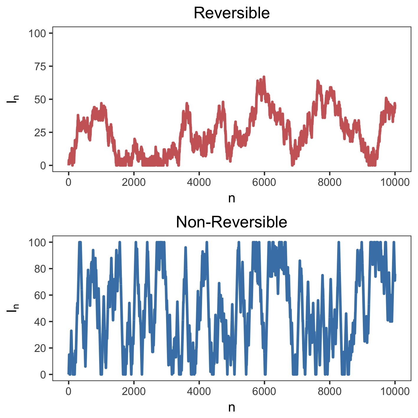
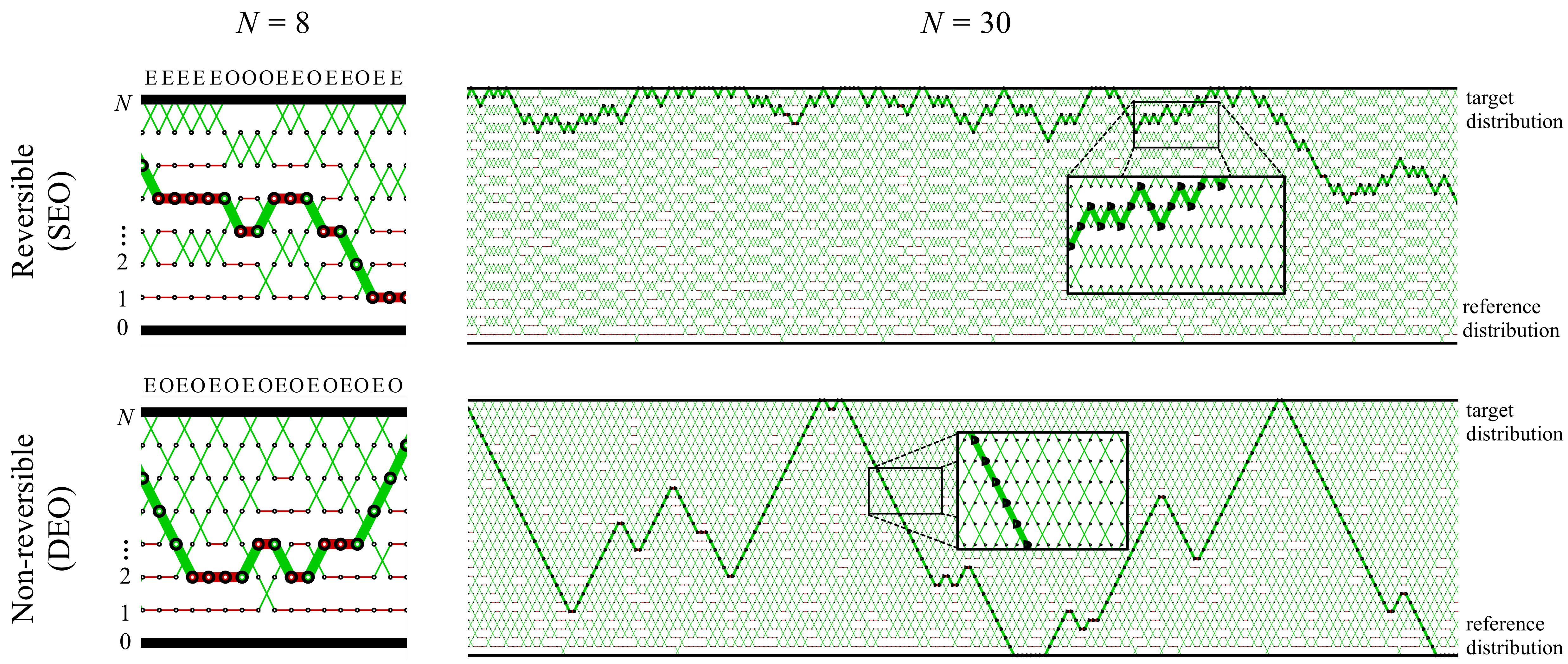
Figure 1: Reversible (top) and non-reversible (bottom) PT for N=8𝑁8N=8 (left) and N=30𝑁30N=30 auxiliary chains (right) using equally spaced annealing parameters on a Bayesian change-point detection model [Davidson-Pilon, 2015] where π0subscript𝜋0\pi_{0} is the prior, π𝜋\pi the posterior. The sequence of swap moves forms N+1𝑁1N+1 index process trajectories (paths formed by the red and green edges). We show one such path in bold. The reversible and non-reversible PT clearly exhibit different scaling behaviour which we formalize in Section 6.

1.1 Parallel Tempering

One popular approach for multi-core and distributed exploration of complex distributions is Parallel Tempering (PT) which was introduced independently in statistics [Geyer, 1991] and physics [Hukushima and Nemoto, 1996]; see also [Swendsen and Wang, 1986] for an earlier related proposal. Since its inception, PT remains to this day a very popular MCMC method to sample from complex multimodal target distributions arising in physics, chemistry, biology, statistics, and machine learning; see, e.g., [Issaoun et al., 2021, Ballnus et al., 2017, Chandra et al., 2019, Cho et al., 2010, Desjardins et al., 2014, Diaz et al., 2020, Dorri et al., 2020, Kamberaj, 2020, Müller and Bouckaert, 2020].

To sample from the target distribution π𝜋\pi, PT introduces a sequence of auxiliary tempered or annealed probability distributions with densities π(βi)(x)L(x)βiπ0(x)proportional-tosuperscript𝜋subscript𝛽𝑖𝑥𝐿superscript𝑥subscript𝛽𝑖subscript𝜋0𝑥\pi^{(\beta_{i})}(x)\propto L(x)^{\beta_{i}}\pi_{0}(x) for i=0,1,,N𝑖01𝑁i=0,1,...,N, where π0subscript𝜋0\pi_{0} is an easy-to-sample reference distribution, L(x)=π(x)/π0(x)𝐿𝑥𝜋𝑥subscript𝜋0𝑥L(x)=\pi(x)/\pi_{0}(x) and the sequence 0=β0<β1<<βN=10subscript𝛽0subscript𝛽1subscript𝛽𝑁10=\beta_{0}<\beta_{1}<\cdots<\beta_{N}=1 defines the annealing schedule. This bridge of auxiliary distributions is used to progressively transform samples from the reference distribution (β=0𝛽0\beta=0) into samples from the target distribution (β=1𝛽1\beta=1), for which only poorly mixing MCMC kernels may be available. For example, in the Bayesian setting where the target distribution is the posterior, we can choose the reference distribution as the prior, from which we can often obtain independent samples.

More precisely, PT algorithms are based on Markov chains in which the states are (N+1)𝑁1(N+1)-tuples, x=(x0,x1,x2,,xN)𝒳N+1xsuperscript𝑥0superscript𝑥1superscript𝑥2superscript𝑥𝑁superscript𝒳𝑁1\textbf{x}=(x^{0},x^{1},x^{2},\dots,x^{N})\in\mathcal{X}^{N+1}, and whose stationary distribution is given by 𝝅(x)=i=0Nπ(βi)(xi)𝝅xsuperscriptsubscriptproduct𝑖0𝑁superscript𝜋subscript𝛽𝑖superscript𝑥𝑖\boldsymbol{\pi}(\textbf{x})=\prod_{i=0}^{N}\pi^{(\beta_{i})}(x^{i}) [Geyer, 1991]. At each iteration, PT proceeds by applying in parallel N+1𝑁1N+1 MCMC kernels targeting π(βi)superscript𝜋subscript𝛽𝑖\pi^{(\beta_{i})} for i=0,,N𝑖0𝑁i=0,...,N. We call these model-specific kernels the local exploration kernels. The chains closer to the reference chain (i.e. those with annealing parameter βisubscript𝛽𝑖\beta_{i} close to zero) can typically traverse regions of low probability mass under π𝜋\pi while the chain at β=1𝛽1\beta=1 ensures that asymptotically we obtain samples from the target distribution. Frequent communication between the chains at the two ends of the spectrum is therefore critical for good performance, and achieved by proposing to swap the states of chains at adjacent annealing parameters. Even swap moves (rows labelled ‘E’), respectively Odd swap moves (labelled ‘O’), propose to exchange states at chains with an even index i𝑖i, respectively odd index i𝑖i, and i+1𝑖1i+1. These proposals are accepted or rejected according to a Metropolis mechanism.

1.2 Deterministic and stochastic even-odd schemes

A key notion used to analyze the behaviour of PT is the index process. To provide intuition on this process, it is helpful to discuss briefly how PT is distributed over several machines. An important point is that instead of having pairs of machines exchanging high-dimensional states when a swap is accepted (which could be detrimental due to network latency), the machines should just exchange the annealing parameters. Suppose now we initialize machine j𝑗j with annealing parameter βjsubscript𝛽𝑗\beta_{j}. Then after n𝑛n scans, the annealing parameters are permuted among the N+1𝑁1N+1 machines according to the permutation In=(In0,,InN)subscriptI𝑛superscriptsubscript𝐼𝑛0superscriptsubscript𝐼𝑛𝑁\textbf{I}_{n}=(I_{n}^{0},\dots,I_{n}^{N}) of {0,,N}0𝑁\{0,\dots,N\}, so that machine j𝑗j has annealing parameter βInjsubscript𝛽superscriptsubscript𝐼𝑛𝑗\beta_{I_{n}^{j}} at iteration n𝑛n of PT. Each index process Injsuperscriptsubscript𝐼𝑛𝑗I_{n}^{j}, formally introduced in Section 2.4, is initialized using I0j=jsubscriptsuperscript𝐼𝑗0𝑗I^{j}_{0}=j and tracks how the state of the corresponding chain evolves over the annealing schedule thanks to the swap moves; see Figure 1. The index process Injsuperscriptsubscript𝐼𝑛𝑗I_{n}^{j} thus monitors the information transfer between the reference and target on machine j𝑗j and as such determines partly the effectiveness of PT.

There have been many proposals made to improve this information transfer by adjusting the annealing schedule; see, e.g., [Kone and Kofke, 2005, Atchadé et al., 2011, Miasojedow et al., 2013]. These proposals are useful but do not address a crucial limitation of standard PT algorithms. In a distributed context, one can select randomly at each iteration whether to apply Even or Odd swap moves in parallel. The resulting stochastic even-odd swap (SEO) scheme, henceforth referred to as reversible PT as it admits a reversible scaling limit (see Section 6), yields index processes exhibiting a diffusive behaviour; see top row of Figure 1. Hence we can expect that when N𝑁N is large it takes roughly O(N2)𝑂superscript𝑁2O(N^{2}) swap attempts for a state at β0=0subscript𝛽00\beta_{0}=0 to reach βN=1subscript𝛽𝑁1\beta_{N}=1 [Diaconis et al., 2000]. The user thus faces a trade-off. If N𝑁N is too large, the acceptance probabilities of the swap moves are high but it takes a time of order O(N2)𝑂superscript𝑁2O(N^{2}) for a state at β=0𝛽0\beta=0 to reach β=1𝛽1\beta=1. If N𝑁N is too low, the acceptance probabilities of swap moves deteriorate resulting in poor mixing between the different chains. Informally, even in a multi-core or distributed setting, for N𝑁N large, the O(N)𝑂𝑁O(N) gains in being able to harness more cores do not offset the O(N2)𝑂superscript𝑁2O(N^{2}) cost of the diffusion (see Section 3.5 where we formalize this argument). As a consequence, the general consensus is that the temperatures should be chosen to allow for about a 20–40% acceptance rate to maximize the squared jump distance travelled per swap in the space of annealing parameters [0,1]01[0,1] [Rathore et al., 2005, Kone and Kofke, 2005, Lingenheil et al., 2009, Atchadé et al., 2011]. Adding more chains past this threshold actually deteriorates the performance of reversible PT and there have even been attempts to adaptively reduce the number of additional chains [Łacki and Miasojedow, 2016]. This is a lost opportunity, since PT is otherwise particularly suitable to implementation on multi-core or distributed architectures.

An alternative to the SEO scheme is the deterministic even-odd swap (DEO) scheme introduced in [Okabe et al., 2001] where one deterministically alternates Even and Odd swap moves. We refer to DEO as non-reversible PT as it admits a non-reversible scaling limit (see Section 6). In particular, the resulting index processes do not appear to exhibit a diffusive, i.e. random walk type, behaviour, illustrated by the bottom row of Figure 1. This non-diffusive behaviour of non-reversible PT explains its excellent empirical performance when compared to alternative reversible PT schemes observed in practice [Lingenheil et al., 2009] for any given schedule. However non-reversible PT, like reversible PT, is sensitive to the choice of the schedule. All the aforementioned tuning strategies developed for PT implicitly assume a reversible framework and do not apply to non-reversible PT (as empirically verified in [Lingenheil et al., 2009]). The main contribution of this paper is to identify some of the theoretical properties of non-reversible PT so as to establish optimal tuning guidelines for this algorithm and propose a novel schedule optimization scheme to implement them. In all our experiments, the resulting iteratively optimized non-reversible PT scheme markedly outperforms the reversible and non-reversible PT schemes currently available (see Section 7).

1.3 Overview of our contributions

After introducing formally the SEO and DEO schemes in Section 2, our first contribution is a non-asymptotic result showing that the non-reversible DEO scheme is guaranteed to outperform its reversible SEO counterpart. The notion of optimality we analyze is the round trip rate, which quantifies how often information from the reference distribution percolates to the target; see Section 3. The theoretical analysis is based on a simplifying assumption called Efficient Local Exploration (ELE), which is not expected to hold exactly in real scenarios. However we show empirically that there are practical methods to approximate ELE and that even when ELE is violated the key predictions made by the theory closely match empirical behaviour. In this sense ELE can be thought of as a useful model for understanding PT algorithms.

In Section 4 we introduce the local and global communication barrier λ(β),Λ𝜆𝛽Λ\lambda(\beta),\Lambda which encode the local and global efficiency of PT. We then show that for non-reversible PT the round trip rate converges to (2+2Λ)1superscript22Λ1(2+2\Lambda)^{-1}, in contrast to the reversible counterpart for which it decays to zero. To provide some intuition on how the small algorithmic difference between SEO and DEO can have such a profound impact, consider the scenario where PT would use the same distributions at the two end-points, π=π0𝜋subscript𝜋0\pi=\pi_{0}, as well as for all intermediate distributions so that Λ=0Λ0\Lambda=0. Clearly this is not a realistic scenario, but in this simple context the index processes of DEO and SEO are easy to describe and contrast. In both DEO and SEO, π=π0𝜋subscript𝜋0\pi=\pi_{0} implies that all proposed swaps will be accepted. For DEO, this makes the index process fully deterministic, performing direct trips from index 00 to N𝑁N and back. Such a process could be compared to a “conveyor belt” with the property that no matter what is the value of N𝑁N, one novel trip from chain 00 reaches chain N𝑁N every two iterations, i.e. the round trip rate is (2+2Λ)1=1/2superscript22Λ112(2+2\Lambda)^{-1}=1/2 as Λ=0Λ0\Lambda=0. For SEO, even when π=π0𝜋subscript𝜋0\pi=\pi_{0} the index process is still random and can be readily seen to be a simple discrete random walk. This implies that as N𝑁N increases, the round trip rate decreases to zero.

In practice, achieving high round trip rates requires careful tuning of the annealing schedule. In Section 5 we combine the analysis from Section 3 and Section 4 to develop a novel methodology to optimize the annealing parameters. The optimal tuning guidelines we provide are different from existing (reversible) PT guidelines and the novel methodology is highly parallel as its performance does not collapse when a very large number of chains is used. However using a large number of chains does have a diminishing return, therefore we propose a mechanism to determine the optimal trade-off between the number of chains and the number of independent PT algorithms one should use.

In Section 6 we identify the scaling limit of the index processes for both reversible and non-reversible PT as the number of parallel chains goes to infinity. We show that this scaling limit is a piecewise-deterministic Markov process for non-reversible PT whereas it is a diffusion for reversible PT as suggested by the dynamics of the bold paths in Figure 1.

Finally in Section 7, we present a variety of experiments validating our theoretical analysis and novel methodology. The method is implemented in an open source Bayesian modelling language available at https://github.com/UBC-Stat-ML/blangSDK. Our software implementation allows the user to specify the model in BUGS-like language [Lunn et al., 2000]. From this model declaration, a suitable sequence of annealed distributions is instantiated and a schedule optimized using our iterative method.

2 Setup and notation

2.1 Parallel tempering

Henceforth we will assume that the target and reference probability distributions π𝜋\pi and π0subscript𝜋0\pi_{0} on 𝒳𝒳\mathcal{X} admit strictly positive densities with respect to a common dominating measure dxd𝑥\mathrm{d}x. We will also denote these densities somewhat abusively by π𝜋\pi and π0subscript𝜋0\pi_{0}. It will be useful to define V0(x)=logπ0(x)subscript𝑉0𝑥subscript𝜋0𝑥V_{0}(x)=-\log\pi_{0}(x) and V(x)=logL(x)𝑉𝑥𝐿𝑥V(x)=-\log L(x), where L(x)=π(x)/π0(x)𝐿𝑥𝜋𝑥subscript𝜋0𝑥L(x)=\pi(x)/\pi_{0}(x) is assumed finite for all x𝒳𝑥𝒳x\in\mathcal{X}. Using this notation, the annealed distribution at an annealing parameter β𝛽\beta is given by

π(β)(x)=L(x)βπ0(x)𝒵(β)=eβV(x)V0(x)𝒵(β),superscript𝜋𝛽𝑥𝐿superscript𝑥𝛽subscript𝜋0𝑥𝒵𝛽superscript𝑒𝛽𝑉𝑥subscript𝑉0𝑥𝒵𝛽\displaystyle\pi^{(\beta)}(x)=\frac{L(x)^{\beta}\pi_{0}(x)}{\mathcal{Z}(\beta)}=\frac{e^{-\beta V(x)-V_{0}(x)}}{\mathcal{Z}(\beta)}, (1)

where 𝒵(β)=𝒳L(x)βπ0(x)dx𝒵𝛽subscript𝒳𝐿superscript𝑥𝛽subscript𝜋0𝑥differential-d𝑥\mathcal{Z}(\beta)=\int_{\mathcal{X}}L(x)^{\beta}\pi_{0}(x)\mathrm{d}x is the corresponding normalizing constant. We denote the annealing schedule by 0=β0<β1<<βN=10subscript𝛽0subscript𝛽1subscript𝛽𝑁10=\beta_{0}<\beta_{1}<\cdots<\beta_{N}=1. In our analysis we will view it as a partition 𝒫N={β0,,βN}subscript𝒫𝑁subscript𝛽0subscript𝛽𝑁\mathcal{P}_{N}=\{\beta_{0},\dots,\beta_{N}\} of [0,1]01[0,1] with mesh-size 𝒫N=supi{βiβi1}normsubscript𝒫𝑁subscriptsupremum𝑖subscript𝛽𝑖subscript𝛽𝑖1\|\mathcal{P}_{N}\|=\sup_{i}\leavevmode\nobreak\ \{\beta_{i}-\beta_{i-1}\}.

We define the PT state x¯=(x,i)¯xxi\bar{\textbf{x}}=(\textbf{x},\textbf{i}) where x=(x0,,xN)𝒳N+1xsuperscript𝑥0superscript𝑥𝑁superscript𝒳𝑁1\textbf{x}=(x^{0},\dots,x^{N})\in\mathcal{X}^{N+1} and i=(i0,,iN)Perm(N)isuperscript𝑖0superscript𝑖𝑁Perm𝑁\textbf{i}=(i^{0},\dots,i^{N})\in\textrm{Perm}(N) the group of permutations on {0,,N}0𝑁\{0,\dots,N\}. PT involves constructing a Markov Chain X¯n=(Xn,In)subscript¯X𝑛subscriptX𝑛subscriptI𝑛\bar{\textbf{X}}_{n}=(\textbf{X}_{n},\textbf{I}_{n}) over 𝒳N+1×Perm(N)superscript𝒳𝑁1Perm𝑁\mathcal{X}^{N+1}\times\textrm{Perm}(N) invariant with respect to 𝝅¯(x¯)=(N+1)!1i=0Nπ(βi)(xi)¯𝝅¯xsuperscript𝑁11superscriptsubscriptproduct𝑖0𝑁superscript𝜋subscript𝛽𝑖superscript𝑥𝑖\bar{\boldsymbol{\pi}}(\bar{\textbf{x}})=(N+1)!^{-1}\prod_{i=0}^{N}\pi^{(\beta_{i})}(x^{i}). The i𝑖i-th component of Xn=(Xn0,,XnN)subscriptX𝑛superscriptsubscript𝑋𝑛0superscriptsubscript𝑋𝑛𝑁\textbf{X}_{n}=(X_{n}^{0},\dots,X_{n}^{N}) tracks the states associated with annealing parameter βisubscript𝛽𝑖\beta_{i} at iteration n𝑛n while the permutation In=(In0,,InN)subscriptI𝑛superscriptsubscript𝐼𝑛0superscriptsubscript𝐼𝑛𝑁\textbf{I}_{n}=(I_{n}^{0},\dots,I_{n}^{N}) tracks how the annealing parameters are shuffled among machines. In particular at iteration n𝑛n, machine j𝑗j stores the Injsubscriptsuperscript𝐼𝑗𝑛I^{j}_{n}-th component of XnsubscriptX𝑛\textbf{X}_{n} and annealing parameter βInjsubscript𝛽superscriptsubscript𝐼𝑛𝑗\beta_{I_{n}^{j}}. The sequence of states associated with βisubscript𝛽𝑖\beta_{i} is called the i𝑖i-th chain and the state on machine j𝑗j is the j𝑗j-th replica.

For both SEO and DEO, the overall 𝝅¯¯𝝅\bar{\boldsymbol{\pi}}-invariant Markov kernel KnPTsubscriptsuperscriptKPT𝑛{\textbf{K}}^{\textrm{PT}}_{n} describing the algorithm is obtained by the composition of a 𝝅¯¯𝝅\bar{\boldsymbol{\pi}}-invariant local exploration kernel KexplsuperscriptKexpl{\textbf{K}}^{\textrm{expl}} and communication kernel KncommsubscriptsuperscriptKcomm𝑛{\textbf{K}}^{\textrm{comm}}_{n},

KnPT(x¯,A)=KncommKexpl(x¯,A):=Kncomm(x¯,dx¯)Kexpl(x¯,A).subscriptsuperscriptKPT𝑛¯x𝐴subscriptsuperscriptKcomm𝑛superscriptKexpl¯x𝐴assignsubscriptsuperscriptKcomm𝑛¯xdsuperscript¯xsuperscriptKexplsuperscript¯x𝐴{\textbf{K}}^{\textrm{PT}}_{n}(\bar{\textbf{x}},A)={\textbf{K}}^{\textrm{comm}}_{n}{\textbf{K}}^{\textrm{expl}}(\bar{\textbf{x}},A):=\int{\textbf{K}}^{\textrm{comm}}_{n}(\bar{\textbf{x}},\textrm{d}\bar{\textbf{x}}^{\prime}){\textbf{K}}^{\textrm{expl}}(\bar{\textbf{x}}^{\prime},A). (2)

The difference between SEO and DEO is in the communication phase, namely Kncomm=KSEOsubscriptsuperscriptKcomm𝑛superscriptKSEO{\textbf{K}}^{\textrm{comm}}_{n}={\textbf{K}}^{\textrm{SEO}} in the former case and Kncomm=KnDEOsubscriptsuperscriptKcomm𝑛subscriptsuperscriptKDEO𝑛{\textbf{K}}^{\textrm{comm}}_{n}={\textbf{K}}^{\textrm{DEO}}_{n} in the latter. Markov kernels corresponding to the reversible (SEO) and non-reversible (DEO) PT algorithms are described informally in the introduction and illustrated in Figure 1.

2.2 Local exploration kernels

The local exploration kernels are defined in the same way for SEO and DEO. They are also model specific, so we assume we are given one π(βi)superscript𝜋subscript𝛽𝑖\pi^{(\beta_{i})}-invariant kernel K(βi)superscript𝐾subscript𝛽𝑖K^{(\beta_{i})} for each annealing parameter βi𝒫Nsubscript𝛽𝑖subscript𝒫𝑁\beta_{i}\in\mathcal{P}_{N}. These can be based on nexplsubscript𝑛expln_{\textrm{expl}} steps of Hamiltonian Monte Carlo, Metropolis–Hastings, Gibbs Sampling, Slice Sampling, etc. We construct the overall local exploration kernel by applying the annealing parameter specific kernels to each component independently from each other:

Kexpl((x,i),A0×A1×AN×{i})=i=0NK(βi)(xi,Ai)δi(i),superscriptKexplxisubscript𝐴0subscript𝐴1subscript𝐴𝑁superscriptisuperscriptsubscriptproduct𝑖0𝑁superscript𝐾subscript𝛽𝑖superscript𝑥𝑖subscript𝐴𝑖subscript𝛿isuperscripti{\textbf{K}}^{\textrm{expl}}((\textbf{x},\textbf{i}),A_{0}\times A_{1}\times\dots A_{N}\times\{\textbf{i}^{\prime}\})=\prod_{i=0}^{N}K^{(\beta_{i})}(x^{i},A_{i})\delta_{\textbf{i}}(\textbf{i}^{\prime}), (3)

where δisubscript𝛿i\delta_{\textbf{i}} denotes the Dirac delta.

In our computational model, we implicitly assume that the local exploration kernel at β=0𝛽0\beta=0 is special in that it can provide independent exact samples from π0subscript𝜋0\pi_{0}. Mathematically, K(0)(x,A0)=π0(A0)superscript𝐾0𝑥subscript𝐴0subscript𝜋0subscript𝐴0K^{(0)}(x,A_{0})=\pi_{0}(A_{0}). This assumption is satisfied in most Bayesian models equipped with proper prior distributions, but also in other situations such as Markov random fields (see Appendix I.6).

2.3 Communication kernels.

Before defining the communication scheme, we first construct its fundamental building block, a swap. A swap is a Metropolis–Hastings move with a deterministic proposal which consists of swapping βisubscript𝛽𝑖\beta_{i} and βi+1subscript𝛽𝑖1\beta_{i+1} across machines. From a current state x¯=(x,i)¯xxi\bar{\textbf{x}}=(\textbf{x},\textbf{i}), a proposed swap state is denoted x¯(i,i+1)=(x(i,i+1),i(i,i+1))superscript¯x𝑖𝑖1superscriptx𝑖𝑖1superscripti𝑖𝑖1\bar{\textbf{x}}^{(i,i+1)}=(\textbf{x}^{(i,i+1)},\textbf{i}^{(i,i+1)}) where

x(i,i+1)superscriptx𝑖𝑖1\displaystyle\textbf{x}^{(i,i+1)} =(x0,,xi1,xi+1,xi,xi+2,,xN),absentsuperscript𝑥0superscript𝑥𝑖1superscript𝑥𝑖1superscript𝑥𝑖superscript𝑥𝑖2superscript𝑥𝑁\displaystyle=(x^{0},\dots,x^{i-1},x^{i+1},x^{i},x^{i+2},\dots,x^{N}), (4)

and i(i,i+1)Perm(N)superscripti𝑖𝑖1Perm𝑁\textbf{i}^{(i,i+1)}\in\textrm{Perm}(N) is the permutation obtained by swapping i𝑖i and i+1𝑖1i+1 in i. The Metropolis–Hastings kernel K(i,i+1)superscriptK𝑖𝑖1\textbf{K}^{(i,i+1)} corresponding to this update is given by

K(i,i+1)(x¯,)=(1α(i,i+1)(x¯))δx¯()+α(i,i+1)(x¯)δx¯(i,i+1)().superscriptK𝑖𝑖1¯x1superscript𝛼𝑖𝑖1¯xsubscript𝛿¯xsuperscript𝛼𝑖𝑖1¯xsubscript𝛿superscript¯x𝑖𝑖1\textbf{K}^{(i,i+1)}(\bar{\textbf{x}},\cdot)=(1-\alpha^{(i,i+1)}(\bar{\textbf{x}}))\delta_{\bar{\textbf{x}}}(\cdot)+\alpha^{(i,i+1)}(\bar{\textbf{x}})\delta_{\bar{\textbf{x}}^{(i,i+1)}}(\cdot). (5)

The function α(i,i+1)(x¯)superscript𝛼𝑖𝑖1¯x\alpha^{(i,i+1)}(\bar{\textbf{x}}) is the corresponding acceptance probability equal to

α(i,i+1)(x¯)superscript𝛼𝑖𝑖1¯x\displaystyle\alpha^{(i,i+1)}(\bar{\textbf{x}}) =min{1,𝝅¯(x¯(i,i+1))𝝅¯(x¯)}=exp(min{0,(βi+1βi)(V(xi+1)V(xi))})absent1¯𝝅superscript¯x𝑖𝑖1¯𝝅¯x0subscript𝛽𝑖1subscript𝛽𝑖𝑉superscript𝑥𝑖1𝑉superscript𝑥𝑖\displaystyle=\min\left\{1,\frac{\bar{\boldsymbol{\pi}}\left(\bar{\textbf{x}}^{(i,i+1)}\right)}{\bar{\boldsymbol{\pi}}(\bar{\textbf{x}})}\right\}=\exp\left(\min\{0,(\beta_{i+1}-\beta_{i})(V(x^{i+1})-V(x^{i}))\}\right) (6)

and the maximal collection of adjacent swap kernels that can be proposed in parallel without interference are

Keven=i evenK(i,i+1),Kodd=i oddK(i,i+1),formulae-sequencesuperscriptKevensubscriptproduct𝑖 evensuperscriptK𝑖𝑖1superscriptKoddsubscriptproduct𝑖 oddsuperscriptK𝑖𝑖1{\textbf{K}}^{\textrm{even}}=\prod_{i\text{ even}}{\textbf{K}}^{(i,i+1)},\qquad{\textbf{K}}^{\textrm{odd}}=\prod_{i\text{ odd}}{\textbf{K}}^{(i,i+1)}, (7)

which we call the even and odd kernels respectively.

For SEO, the kernel Kncomm=KSEOsubscriptsuperscriptKcomm𝑛superscriptKSEO{\textbf{K}}^{\textrm{comm}}_{n}={\textbf{K}}^{\textrm{SEO}} is given by a mixture of the even and odd kernels in equal proportion while for DEO the kernel Kncomm=KnDEOsubscriptsuperscriptKcomm𝑛subscriptsuperscriptKDEO𝑛{\textbf{K}}^{\textrm{comm}}_{n}={\textbf{K}}^{\textrm{DEO}}_{n} is given by a deterministic alternation between even and odd kernels, that is

KSEO=12Keven+12Kodd,KnDEO={Kevenif n is even,Koddif n is odd.formulae-sequencesuperscriptKSEO12superscriptKeven12superscriptKoddsubscriptsuperscriptKDEO𝑛casessuperscriptKevenif n is even,superscriptKoddif n is odd.{\textbf{K}}^{\textrm{SEO}}=\frac{1}{2}{\textbf{K}}^{\textrm{even}}+\frac{1}{2}{\textbf{K}}^{\textrm{odd}},\quad\quad{\textbf{K}}^{\textrm{DEO}}_{n}=\begin{cases}{\textbf{K}}^{\textrm{even}}&\text{if $n$ is even,}\\ {\textbf{K}}^{\textrm{odd}}&\text{if $n$ is odd.}\end{cases} (8)

We provide pseudo-code for the DEO scheme in Algorithm 1. The pseudo-code also estimates the average rejection probabilities r(i,i+1)superscript𝑟𝑖𝑖1r^{(i,i+1)} of swap moves between chains i𝑖i and i+1𝑖1i+1 which are used to optimize the annealing schedule in Section 5. When the schedule is fixed, lines 1, 12, 17 can be omitted, and one should use “for iP𝑖𝑃i\in P” on line 10. For simplicity, the swap in line 15 is shown for a parallel computing context, where several cores have a shared memory, and hence line 15 is simply an exchange of pointers in an array, which is efficient thanks to memory sharing. For a distributed computing implementation, where several machines do not share memory and instead need to communicate over the network, it becomes advantageous to swap annealing parameters instead of states. Refer to Appendix H for pseudo-code for the distributed computing implementation.

Algorithm 1 DEO(number of scans nscansubscript𝑛scann_{\textrm{scan}}, annealing schedule 𝒫Nsubscript𝒫𝑁\mathcal{P}_{N})
1:r(i,i+1)0superscript𝑟𝑖𝑖10r^{(i,i+1)}\leftarrow 0 for all i{0,1,,N1}𝑖01𝑁1i\in\{0,1,\dots,N-1\} \triangleright Swap rejection statistics used in Section 5.4 to optimize the schedule
2:xx0xsubscriptx0\textbf{x}\leftarrow\textbf{x}_{0} \triangleright Initialize chain
3:for n𝑛n in 1, 2, …, nscansubscript𝑛scann_{\textrm{scan}} do
4:     if n𝑛n is even then \triangleright Non-reversibility inducing alternation
5:         P{i:0i<N,i is even}𝑃conditional-set𝑖formulae-sequence0𝑖𝑁𝑖 is evenP\leftarrow\{i:0\leq i<N,i\text{ is even}\} \triangleright Even subset of {0,,N1}0𝑁1\{0,\dots,N-1\}
6:     else
7:         P{i:0i<N,i is odd}𝑃conditional-set𝑖formulae-sequence0𝑖𝑁𝑖 is oddP\leftarrow\{i:0\leq i<N,i\text{ is odd}\} \triangleright Odd subset of {0,,N1}0𝑁1\{0,\dots,N-1\}      
8:     for i𝑖i in 0,,N0𝑁0,\dots,N do \triangleright Local exploration phase (parallelizable)
9:         xiK(βi)(xn1i,)similar-tosuperscript𝑥𝑖superscript𝐾subscript𝛽𝑖subscriptsuperscript𝑥𝑖𝑛1x^{i}\sim K^{(\beta_{i})}(x^{i}_{n-1},\cdot)      
10:     for i𝑖i in 0,,N10𝑁10,\dots,N-1 do \triangleright Communication phase (parallelizable)
11:         αα(i,i+1)𝛼superscript𝛼𝑖𝑖1\alpha\leftarrow\alpha^{(i,i+1)} \triangleright Equation (6).
12:         r(i,i+1)r(i,i+1)+(1α)superscript𝑟𝑖𝑖1superscript𝑟𝑖𝑖11𝛼r^{(i,i+1)}\leftarrow r^{(i,i+1)}+(1-\alpha)
13:         ABern(α)similar-to𝐴Bern𝛼A\sim\mathrm{Bern}(\alpha)
14:         if iP𝑖𝑃i\in P and A=1𝐴1A=1 then
15:              (xi,xi+1)(xi+1,xi)superscript𝑥𝑖superscript𝑥𝑖1superscript𝑥𝑖1superscript𝑥𝑖(x^{i},x^{i+1})\leftarrow(x^{i+1},x^{i}) \triangleright See also Appendix H for a distributed computing implementation, where annealing parameters are swapped instead of states.               
16:     xnxsubscriptx𝑛x\textbf{x}_{n}\leftarrow\textbf{x}
17:r(i,i+1)r(i,i+1)/nscansuperscript𝑟𝑖𝑖1superscript𝑟𝑖𝑖1subscript𝑛scanr^{(i,i+1)}\leftarrow r^{(i,i+1)}/n_{\textrm{scan}} for all i{0,1,,N1}𝑖01𝑁1i\in\{0,1,\dots,N-1\}\triangleright Equation (31)
18:return (x1,,xnscan),(r(0,1),,r(N1,N))subscriptx1subscriptxsubscript𝑛scansuperscript𝑟01superscript𝑟𝑁1𝑁(\textbf{x}_{1},\dots,\textbf{x}_{n_{\textrm{scan}}}),(r^{(0,1)},\dots,r^{(N-1,N)})

2.4 The index process

As discussed in Section 1.2, the j𝑗j-th component of permutation In=(In0,,InN)subscriptI𝑛subscriptsuperscript𝐼0𝑛subscriptsuperscript𝐼𝑁𝑛\textbf{I}_{n}=(I^{0}_{n},\dots,I^{N}_{n}) encodes the flow of information between the reference and target on machine j𝑗j. We define the index process for machine j𝑗j as (Inj,εnj){0,,N}×{1,1}superscriptsubscript𝐼𝑛𝑗superscriptsubscript𝜀𝑛𝑗0𝑁11(I_{n}^{j},\varepsilon_{n}^{j})\in\{0,\dots,N\}\times\{-1,1\}, where εnj=1superscriptsubscript𝜀𝑛𝑗1\varepsilon_{n}^{j}=1 if the annealing parameter on machine j𝑗j is proposed an increase after scan n𝑛n, and 11-1 otherwise. The concept is best understood visually: refer to the bold piecewise linear paths illustrating InN2subscriptsuperscript𝐼𝑁2𝑛I^{N-2}_{n} for N=8𝑁8N=8 and InN1subscriptsuperscript𝐼𝑁1𝑛I^{N-1}_{n} for N=30𝑁30N=30 in Figure 1.

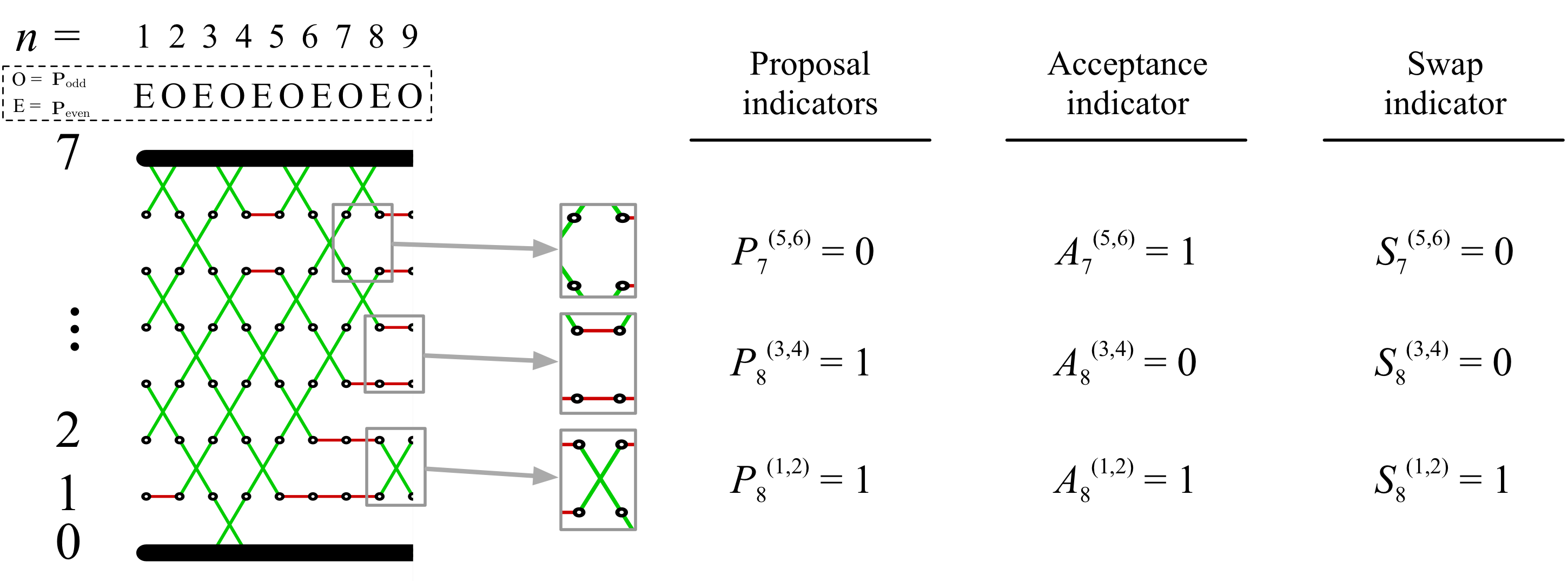
Let P(i,i+1){0,1}superscript𝑃𝑖𝑖101P^{(i,i+1)}\in\{0,1\} denote an indicator that a swap is proposed between chains i𝑖i and i+1𝑖1i+1 at iteration n𝑛n. The realized swaps are then defined from the proposal indicators as S(i,i+1)=P(i,i+1)A(i,i+1)superscript𝑆𝑖𝑖1superscript𝑃𝑖𝑖1superscript𝐴𝑖𝑖1S^{(i,i+1)}=P^{(i,i+1)}A^{(i,i+1)}, where A(i,i+1)|X¯Bern(α(i,i+1)(X¯))similar-toconditionalsuperscript𝐴𝑖𝑖1¯XBernsuperscript𝛼𝑖𝑖1¯XA^{(i,i+1)}|\bar{\textbf{X}}\sim\mathrm{Bern}(\alpha^{(i,i+1)}(\bar{\textbf{X}})) are acceptance indicator variables (Figure 2 in Appendix J). The index process satisfies the following recursive relation: initialize I0j=jsubscriptsuperscript𝐼𝑗0𝑗I^{j}_{0}=j and ε0j=1superscriptsubscript𝜀0𝑗1\varepsilon_{0}^{j}=1 if P0(j,j+1)=1superscriptsubscript𝑃0𝑗𝑗11P_{0}^{(j,j+1)}=1 and 11-1 otherwise. For n>0𝑛0n>0, we have

In+1jsuperscriptsubscript𝐼𝑛1𝑗\displaystyle I_{n+1}^{j} ={Inj+εnjif Sn(Inj,Inj+εnj)=1,Injotherwise,,εn+1jabsentcasessuperscriptsubscript𝐼𝑛𝑗superscriptsubscript𝜀𝑛𝑗if superscriptsubscript𝑆𝑛superscriptsubscript𝐼𝑛𝑗superscriptsubscript𝐼𝑛𝑗superscriptsubscript𝜀𝑛𝑗1superscriptsubscript𝐼𝑛𝑗otherwisesuperscriptsubscript𝜀𝑛1𝑗\displaystyle=\begin{cases}I_{n}^{j}+\varepsilon_{n}^{j}&\text{if }S_{n}^{(I_{n}^{j},I_{n}^{j}+\varepsilon_{n}^{j})}=1,\\ I_{n}^{j}&\text{otherwise},\end{cases},\qquad\varepsilon_{n+1}^{j} ={1if Pn(In+1j,In+1j+1)=1,1otherwise.absentcases1if superscriptsubscript𝑃𝑛superscriptsubscript𝐼𝑛1𝑗superscriptsubscript𝐼𝑛1𝑗111otherwise.\displaystyle=\begin{cases}1&\text{if }P_{n}^{(I_{n+1}^{j},I_{n+1}^{j}+1)}=1,\\ -1&\text{otherwise.}\end{cases} (9)
Refer to caption
Figure 2: Illustration of the proposal, acceptance and swap indicators.

We will use the dynamics of the index process to explain the differences between SEO and DEO communication. The only difference between the two is in the proposal indicators. Define Pn=(Pn(0,1),Pn(1,2),,Pn(N1,N))subscriptP𝑛superscriptsubscript𝑃𝑛01superscriptsubscript𝑃𝑛12superscriptsubscript𝑃𝑛𝑁1𝑁\textbf{P}_{n}=(P_{n}^{(0,1)},P_{n}^{(1,2)},\dots,P_{n}^{(N-1,N)}), PnsubscriptP𝑛\textbf{P}_{n} is deterministic for DEO, i.e. Pn=Peven=(1,0,1,)subscriptP𝑛subscriptPeven101\textbf{P}_{n}=\textbf{P}_{\text{even}}=(1,0,1,\dots) for even n𝑛n and Pn=Podd=(0,1,0,)subscriptP𝑛subscriptPodd010\textbf{P}_{n}=\textbf{P}_{\text{odd}}=(0,1,0,\dots) for odd n𝑛n. In SEO, we have PnUnif{Peven,Podd}similar-tosubscriptP𝑛UnifsubscriptPevensubscriptPodd\textbf{P}_{n}\sim\text{Unif}\{\textbf{P}_{\text{even}},\textbf{P}_{\text{odd}}\}.

For SEO, the variables εnUnif{1,1}similar-tosubscript𝜀𝑛Unif11\varepsilon_{n}\sim\mathrm{Unif}\{-1,1\} are i.i.d, and consequently the index process exhibits a random walk behaviour. In contrast for DEO, we have εn+1j=εnjsubscriptsuperscript𝜀𝑗𝑛1subscriptsuperscript𝜀𝑗𝑛\varepsilon^{j}_{n+1}=\varepsilon^{j}_{n} so long as In+1j=Inj+εnjsubscriptsuperscript𝐼𝑗𝑛1subscriptsuperscript𝐼𝑗𝑛subscriptsuperscript𝜀𝑗𝑛I^{j}_{n+1}=I^{j}_{n}+\varepsilon^{j}_{n} and εn+1j=εnjsubscriptsuperscript𝜀𝑗𝑛1subscriptsuperscript𝜀𝑗𝑛\varepsilon^{j}_{n+1}=-\varepsilon^{j}_{n} otherwise. Therefore the index process for DEO performs a more systematic exploration of the space as the direction εn+1jsubscriptsuperscript𝜀𝑗𝑛1\varepsilon^{j}_{n+1} is only reversed when a swap involving machine j𝑗j is rejected or if the boundary is reached. The qualitative differences between the two regimes can be seen in Figure 1 (see also Figure 15 in the Supplementary Material). In particular the index process for DEO in these figures behaves very differently as N𝑁N increases, this will be explored formally in Section 6.

As mentioned in the introduction, we refer to the PT algorithm with SEO and DEO communication as reversible PT and non-reversible PT respectively. Our terminology is somewhat abusive but is justified by the analysis in Section 3.4 and Section 6, where it is shown that, under certain assumptions, the index process is reversible for SEO while it is non-reversible for DEO.

3 Non-asymptotic analysis of PT algorithms

3.1 Model of compute time

We start with a definition of what we model as one unit of compute time: throughout the paper, we assume a massively parallel or distributed computational setup and sampling once from each of local exploration kernel K(β)superscript𝐾𝛽K^{(\beta)} has cost O(nexpl)𝑂subscript𝑛explO(n_{\textrm{expl}}) which dominates the cost of the swap kernel K(i,i+1)superscriptK𝑖𝑖1{\textbf{K}}^{(i,i+1)}. Consequently a scan of PT has cost O(nexpl)𝑂subscript𝑛explO(n_{\textrm{expl}}) and for a fixed computational budget ntotalsubscript𝑛totaln_{\textrm{total}}, the total number of scans is nscan=O(ntotal/nexpl)subscript𝑛scan𝑂subscript𝑛totalsubscript𝑛expln_{\textrm{scan}}=O(n_{\textrm{total}}/n_{\textrm{expl}}).

The assumption that the per-iteration cost of PT is independent of the number of chains is reasonable in GPU and parallel computing scenarios, since the communication cost for each swap does not increase with the dimension of the problem (by swapping annealing parameters instead of states). We also assume that the number of PT scans will dominate the number of parallel cores available, i.e. nscanNmuch-greater-thansubscript𝑛scan𝑁n_{\textrm{scan}}\gg N. This is reasonable when addressing challenging sampling problems. Although there are numerous empirical studies on multi-core and distributed implementation of PT [Altekar et al., 2004, Mingas and Bouganis, 2012, Fang et al., 2014], we are not aware of previous theoretical work investigating such a computational model.

3.2 Performance metrics for PT methods

The standard notion of computational efficiency of MCMC schemes is the effective sample size (ESS) per compute time. However, for PT methods, since the ESS per compute time depends on the details of the problem specific local exploration kernels KexplsuperscriptKexpl{\textbf{K}}^{\textrm{expl}}, alternatives have been developed in the literature to assess the performance of KncommsubscriptsuperscriptKcomm𝑛{\textbf{K}}^{\textrm{comm}}_{n} which are independent of KexplsuperscriptKexpl{\textbf{K}}^{\textrm{expl}} [Katzgraber et al., 2006, Lingenheil et al., 2009].

We are motivated by the Bayesian context where it is typically possible to obtain one independent sample from the reference distribution π0subscript𝜋0\pi_{0} (i.e. from the prior distribution) at each iteration. We say that an annealed restart has occurred on machine j𝑗j when Injsuperscriptsubscript𝐼𝑛𝑗I_{n}^{j} goes from 00 to N𝑁N (i.e. β𝛽\beta goes from 00 to 111), which corresponds to a sample generated from π0subscript𝜋0\pi_{0} propagating to the target π𝜋\pi. Informally an annealed restart can be thought of as a sampling equivalent to what is known in optimization as a random restart. We say a round trip has occurred on machine j𝑗j when Injsuperscriptsubscript𝐼𝑛𝑗I_{n}^{j} goes from 00 to N𝑁N and then goes back to 00 (i.e. β𝛽\beta goes from 00 to 111 to 00).

Formally, we recursively define T,0j=inf{n:(Inj,εnj)=(0,1)}superscriptsubscript𝑇0𝑗infimumconditional-set𝑛superscriptsubscript𝐼𝑛𝑗superscriptsubscript𝜀𝑛𝑗01T_{\downarrow,0}^{j}=\inf\{n:(I_{n}^{j},\varepsilon_{n}^{j})=(0,-1)\} and for k1𝑘1k\geq 1,

T,kjsuperscriptsubscript𝑇𝑘𝑗\displaystyle T_{\uparrow,k}^{j} =inf{n>T,k1j:(Inj,εnj)=(N,1)},absentinfimumconditional-set𝑛superscriptsubscript𝑇𝑘1𝑗superscriptsubscript𝐼𝑛𝑗superscriptsubscript𝜀𝑛𝑗𝑁1\displaystyle=\inf\{n>T_{\downarrow,k-1}^{j}:(I_{n}^{j},\varepsilon_{n}^{j})=(N,1)\}, (10)
T,kjsuperscriptsubscript𝑇𝑘𝑗\displaystyle T_{\downarrow,k}^{j} =inf{n>T,kj:(Inj,εnj)=(0,1)}.absentinfimumconditional-set𝑛superscriptsubscript𝑇𝑘𝑗superscriptsubscript𝐼𝑛𝑗superscriptsubscript𝜀𝑛𝑗01\displaystyle=\inf\{n>T_{\uparrow,k}^{j}:(I_{n}^{j},\varepsilon_{n}^{j})=(0,-1)\}. (11)

The k𝑘k-th annealed restart and round trip for machine j𝑗j occurs at scan T,kjsuperscriptsubscript𝑇𝑘𝑗T_{\uparrow,k}^{j} and T,kjsuperscriptsubscript𝑇𝑘𝑗T_{\downarrow,k}^{j} respectively. Let 𝒯nsubscript𝒯𝑛\mathcal{T}_{n} and nsubscript𝑛\mathcal{R}_{n} be the total number of annealed restarts and round trips respectively during the first n𝑛n scans of the DEO algorithm.

We wish to optimize for the percentage of iterations that result in an annealed restart, i.e. τ=limn𝔼[𝒯n]/n𝜏subscript𝑛𝔼delimited-[]subscript𝒯𝑛𝑛\tau=\lim_{n\to\infty}{\mathbb{E}}[\mathcal{T}_{n}]/n, where we use abusively the same random variables for SEO and DEO but differentiate these schemes by using the probability measures SEOsubscriptSEO\mathbb{P}_{\textrm{SEO}} and DEOsubscriptDEO\mathbb{P}_{\textrm{DEO}} with associated expectation operators 𝔼SEOsubscript𝔼SEO\mathbb{E}_{\textrm{SEO}} and 𝔼DEOsubscript𝔼DEO\mathbb{E}_{\textrm{DEO}}. We use \mathbb{P} and 𝔼𝔼{\mathbb{E}} for statements that hold for both algorithms. If 𝒯njsuperscriptsubscript𝒯𝑛𝑗\mathcal{T}_{n}^{j} and njsuperscriptsubscript𝑛𝑗\mathcal{R}_{n}^{j} are the total number of annealed restarts and round trips during the first n𝑛n iterations on machine j𝑗j respectively, then we have nj𝒯njnj+1superscriptsubscript𝑛𝑗superscriptsubscript𝒯𝑛𝑗superscriptsubscript𝑛𝑗1\mathcal{R}_{n}^{j}\leq\mathcal{T}_{n}^{j}\leq\mathcal{R}_{n}^{j}+1. Consequently, n𝒯nn+N+1subscript𝑛subscript𝒯𝑛subscript𝑛𝑁1\mathcal{R}_{n}\leq\mathcal{T}_{n}\leq\mathcal{R}_{n}+N+1 and thus τ=limn𝔼[n]/n𝜏subscript𝑛𝔼delimited-[]subscript𝑛𝑛\tau=\lim_{n\to\infty}{\mathbb{E}}[\mathcal{R}_{n}]/n.

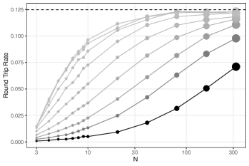
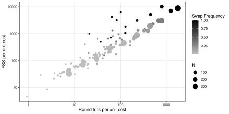
In the PT literature, τ𝜏\tau is commonly referred to as the round trip rate and has been used to compare the effectiveness of various PT algorithms [Katzgraber et al., 2006, Lingenheil et al., 2009]. Empirically we observed that round trips per unit cost strongly correlate with ESS per unit cost as seen in Figure 3, making the round trip rate a natural objective function to compare and tune parallel tempering algorithms.
Refer to caption
Refer to caption
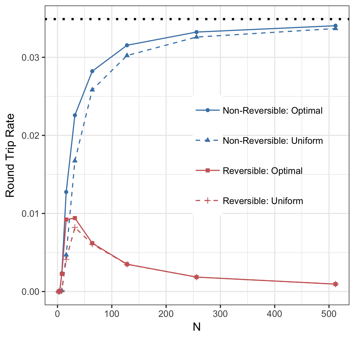
Figure 3: The round trip rate and ESS for a 5×5555\times 5 Ising Model with a magnetic moment 0.10.10.1 and nexplsubscript𝑛expln_{\textrm{expl}} 1-bit flips between scans ranging from 111 to 400400400, and N𝑁N ranging from 333 to 320320320. The schedule is tuned using Algorithm 4 with ntune=25000subscript𝑛tune25000n_{\textrm{tune}}=25000 scans for tuning, nsample=25000subscript𝑛sample25000n_{\textrm{sample}}=25000 scans for sampling. (Left) Round trip rate versus N𝑁N for different swap attempt frequency (1/nexpl)1/n_{\textrm{expl}}). The dotted line is the optimal round trip rate τ¯¯𝜏\bar{\tau} predicted by Theorem 3. (Right) The ESS per unit cost versus round trip rate per unit cost for each run, with a correlation coefficient of 0.81.

Another performance metric commonly used in the PT literature is the expected square jump distance (ESJD) [Atchadé et al., 2011, Kone and Kofke, 2005]. While this criterion is useful within the context of reversible PT for selecting the optimal number of parallel chains, the ESJD is too coarse to compare reversible to non-reversible PT methods as, for any given annealing schedule, the ESJD is identical in both cases.

3.3 Model assumptions

The analysis of the round trip times is in general intractable because the index process is not Markovian. Indeed, simulating a transition depends on the swap indicators Sn(i,i+1)superscriptsubscript𝑆𝑛𝑖𝑖1S_{n}^{(i,i+1)} (see Section 2.4), the distributions of which themselves depend on the state configuration X¯¯X\bar{\textbf{X}}. To simplify the analysis, we will make in the remainder of the paper the following simplifying assumptions:

  1. (A1)

    Stationarity: X¯0𝝅¯similar-tosubscript¯X0¯𝝅\bar{\textbf{X}}_{0}\sim\bar{\boldsymbol{\pi}} and thus X¯n𝝅¯similar-tosubscript¯X𝑛¯𝝅\bar{\textbf{X}}_{n}\sim\bar{\boldsymbol{\pi}} for all n𝑛n as the kernel KnPTsubscriptsuperscriptKPT𝑛{\textbf{K}}^{\textrm{PT}}_{n} is 𝝅¯¯𝝅\bar{\boldsymbol{\pi}}-invariant.

  2. (A2)

    Efficient Local Exploration (ELE): For Xπ(β)similar-to𝑋superscript𝜋𝛽X\sim\pi^{(\beta)} and X|XK(β)(X,)similar-toconditionalsuperscript𝑋𝑋superscript𝐾𝛽𝑋X^{\prime}|X\sim K^{(\beta)}(X,\cdot), the random variables V(X)𝑉𝑋V(X) and V(X)𝑉superscript𝑋V(X^{\prime}) are independent.

  3. (A3)

    Integrability: V3superscript𝑉3V^{3} is integrable with respect to π0subscript𝜋0\pi_{0} and π𝜋\pi.

It follows from Assumptions (A1)–(A2) and (6) that the behaviour of the communication scheme only depends on the distribution of the state X¯nsubscript¯X𝑛\bar{\textbf{X}}_{n} via the N+1𝑁1N+1 univariate distributions of the chain-specific energies V(i)=V(X(i))superscript𝑉𝑖𝑉superscript𝑋𝑖V^{(i)}=V\left(X^{(i)}\right), i{0,1,2,,N}𝑖012𝑁i\in\{0,1,2,\dots,N\}. This allows us to build a theoretical analysis which makes no structural assumption on the state space 𝒳𝒳\mathcal{X} or the target π𝜋\pi as typically done in the literature: for example, [Atchadé et al., 2011] assume a product space 𝒳=𝒳0d𝒳superscriptsubscript𝒳0𝑑\mathcal{X}=\mathcal{X}_{0}^{d} for large d𝑑d, and [Predescu et al., 2004] assume π(β)superscript𝜋𝛽\pi^{(\beta)} satisfies a constant heat capacity.

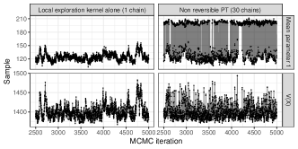
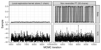
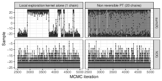
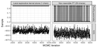
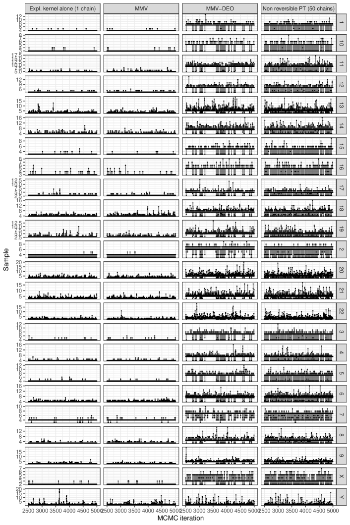
Admittedly the ELE assumption (A2) does not hold in practical applications. ELE can be approximated by increasing the number of local exploration kernels applied between consecutive swap (nexplsubscript𝑛expln_{\textrm{expl}}). However one may worry that to achieve a good approximation in challenging problems, nexplsubscript𝑛expln_{\textrm{expl}} would have to be set to a value so large as to defy the practicality of our analysis. Surprisingly, we have observed empirically that this was not the case in the multimodal problems we considered. Figure 4 displays results in four models where a local exploration kernel alone induces good mixing of the energy chain V(Xn)𝑉subscript𝑋𝑛V(X_{n}) (hence ELE can be approximated) yet the local exploration kernel alone is insufficient to achieve good mixing on the full state space, X¯nsubscript¯X𝑛\bar{\textbf{X}}_{n} (so that PT is justified and indeed yields efficient exploration of the configuration space). This gap is possible since V(X)𝑉𝑋V(X) is 1-dimensional and potentially unimodal even when X𝑋X is not. This is the motivation for ELE since assuming the independence of V(X)𝑉𝑋V(X) and V(X)𝑉superscript𝑋V(X^{\prime}) is weaker than assuming the independence of X𝑋X and Xsuperscript𝑋X^{\prime} (as hypothesized e.g. in Section 5.1 of [Atchadé et al., 2011]). Obviously ELE is still expected to be a somewhat crude simplifying assumption in very complex problems; e.g. for the highly challenging high-dimensional copy number inference problem illustrated in Figure 4.

In Section 7.2, we describe additional empirical results supporting that ELE is a useful model for the purpose of designing and analyzing PT algorithms. In the severe ELE violation regime, we show that the key quantities used in our analysis are either well approximated, or approached as N𝑁N increases.

Bayesian mixture model ODE parameters
Refer to caption Refer to caption
Ising model Copy number inference
Refer to caption Refer to caption
Figure 4: Four multimodal examples (described in Section 7.1 and Appendix I) where a local exploration kernel provides a reasonable approximation of the ELE assumption. For each inference problem, we show trace plots for MCMC based on single chain (i.e. the local exploration kernel alone; left facet), and for a non-reversible PT algorithm based on the same local exploration kernel (right facet). The top facets each show a component of X𝑋X, and the bottom facets, V(X)𝑉𝑋V(X).

Assumptions (A1)-(A2) allow us to express the swap indicators as independent Bernoulli random variables Sn(i,i+1)Bern(s(i,i+1))similar-tosuperscriptsubscript𝑆𝑛𝑖𝑖1Bernsuperscript𝑠𝑖𝑖1S_{n}^{(i,i+1)}\sim\text{Bern}(s^{(i,i+1)}) where s(i,i+1)superscript𝑠𝑖𝑖1s^{(i,i+1)} is given by the expectation of Equation (6),

s(i,i+1)=𝔼[α(i,i+1)(X¯)]=𝔼[exp(min{0,(βi+1βi)(V(i+1)V(i))})],superscript𝑠𝑖𝑖1𝔼delimited-[]superscript𝛼𝑖𝑖1¯X𝔼delimited-[]0subscript𝛽𝑖1subscript𝛽𝑖superscript𝑉𝑖1superscript𝑉𝑖s^{(i,i+1)}={\mathbb{E}}\left[\alpha^{(i,i+1)}(\bar{\textbf{X}})\right]={\mathbb{E}}\left[\exp\left(\min\left\{0,\left(\beta_{i+1}-\beta_{i}\right)\left(V^{(i+1)}-V^{(i)}\right)\right\}\right)\right], (12)

the expectation being over two independent random variables V(i),V(i+1)superscript𝑉𝑖superscript𝑉𝑖1V^{(i)},V^{(i+1)}, satisfying V(i)=dV(X(βi))superscript𝑑superscript𝑉𝑖𝑉superscript𝑋subscript𝛽𝑖V^{(i)}\stackrel{{\scriptstyle d}}{{=}}V(X^{(\beta_{i})}) for X(βi)π(βi)similar-tosuperscript𝑋subscript𝛽𝑖superscript𝜋subscript𝛽𝑖X^{(\beta_{i})}\sim\pi^{(\beta_{i})}.

3.4 Reversibility and non-reversibility of the index process

Under assumptions (A1)-(A2), each index process (Inj,εnj)subscriptsuperscript𝐼𝑗𝑛subscriptsuperscript𝜀𝑗𝑛(I^{j}_{n},\varepsilon^{j}_{n}) is Markovian for j=0,,N𝑗0𝑁j=0,\dots,N with transition kernel KSEOsuperscript𝐾SEOK^{\mathrm{SEO}} and KDEOsuperscript𝐾DEOK^{\mathrm{DEO}} for reversible and non-reversible PT respectively. See Appendix A for an explicit representation of these kernels. We drop the superscript j𝑗j when the particular machine is not relevant.

The kernel KSEOsuperscript𝐾SEOK^{\mathrm{SEO}} defines a reversible Markov chain on {0,,N}×{1,1}0𝑁11\{0,\dots,N\}\times\{-1,1\} with uniform stationary distribution while KDEOsuperscript𝐾DEOK^{\mathrm{DEO}} satisfies the skew-detailed balance condition with respect to the same distribution,

KDEO((i,ε),(i,ε))=KDEO((i,ε),(i,ε)),superscript𝐾DEO𝑖𝜀superscript𝑖superscript𝜀superscript𝐾DEOsuperscript𝑖superscript𝜀𝑖𝜀K^{\mathrm{DEO}}((i,\varepsilon),(i^{\prime},\varepsilon^{\prime}))=K^{\mathrm{DEO}}((i^{\prime},-\varepsilon^{\prime}),(i,-\varepsilon)), (13)

and is thus non-reversible. It falls within the generalized Metropolis–Hastings framework, see, e.g., [Lelièvre et al., 2010].

Reversibility necessitates that the Markov chain must be allowed to backtrack its movements. This leads to inefficient exploration of the state space. As a consequence, non-reversibility is typically a favourable property for MCMC chains. A common recipe to design non-reversible sampling algorithms consists of expanding the state space to include a “lifting” parameter that allows for a more systematic exploration of the state space [Chen et al., 1999, Diaconis et al., 2000, Turitsyn et al., 2011, Vucelja, 2016].

The index process (In,εn)subscript𝐼𝑛subscript𝜀𝑛(I_{n},\varepsilon_{n}) for non-reversible PT can be interpreted as a “lifted” version of the index process for reversible PT with lifting parameter εnsubscript𝜀𝑛\varepsilon_{n}. Under DEO communication, Insubscript𝐼𝑛I_{n} travels in the direction εnsubscript𝜀𝑛\varepsilon_{n} and only reverses direction when Insubscript𝐼𝑛I_{n} reaches a boundary or when a swap rejection occurs. This “lifting” construction helps explain the qualitatively different behaviour between reversible and non-reversible PT and will be further explored when identifying the scaling limit of (In,εn)subscript𝐼𝑛subscript𝜀𝑛(I_{n},\varepsilon_{n}) in Section 6. The lifted PT of [Wu, 2017] exploits a similar construction but only one of the N+1𝑁1N+1 index processes is lifted instead of all of them for DEO. A lifted version of simulated tempering has also been proposed by [Sakai and Hukushima, 2016].

3.5 Non-asymptotic domination of non-reversible PT

Assumptions (A1)-(A2) ensure that for each j=0,,N𝑗0𝑁j=0,\dots,N, njsuperscriptsubscript𝑛𝑗\mathcal{R}_{n}^{j} is a delayed renewal process with round trip times Tkj=T,kjT,k1jsuperscriptsubscript𝑇𝑘𝑗subscriptsuperscript𝑇𝑗𝑘subscriptsuperscript𝑇𝑗𝑘1T_{k}^{j}=T^{j}_{\downarrow,k}-T^{j}_{\downarrow,k-1} for k1𝑘1k\geq 1 and j=0,,N𝑗0𝑁j=0,\dots,N. In particular, Tkjsuperscriptsubscript𝑇𝑘𝑗T_{k}^{j} are independent and identically distributed and, for convenience, we introduce the random variable T=dTkjsuperscript𝑑𝑇superscriptsubscript𝑇𝑘𝑗T\stackrel{{\scriptstyle d}}{{=}}T_{k}^{j}. By the key renewal theorem, we have

τ=j=0Nlimn𝔼[nj]n=N+1𝔼[T].𝜏superscriptsubscript𝑗0𝑁subscript𝑛𝔼delimited-[]subscriptsuperscript𝑗𝑛𝑛𝑁1𝔼delimited-[]𝑇\displaystyle\tau=\sum_{j=0}^{N}\lim_{n\to\infty}\frac{{\mathbb{E}}[\mathcal{R}^{j}_{n}]}{n}=\frac{N+1}{{\mathbb{E}}[T]}. (14)

An analytical expression for 𝔼[T]𝔼delimited-[]𝑇{\mathbb{E}}[T] for reversible PT was first derived by [Nadler and Hansmann, 2007]. We extend this result to non-reversible PT in Theorem 1.

Theorem 1.

For any annealing schedule 𝒫N={β0,,βN}subscript𝒫𝑁subscript𝛽0subscript𝛽𝑁\mathcal{P}_{N}=\{\beta_{0},\dots,\beta_{N}\},

𝔼SEO[T]subscript𝔼SEOdelimited-[]𝑇\displaystyle{\mathbb{E}}_{\mathrm{SEO}}[T] =2(N+1)N+2(N+1)E(𝒫N),absent2𝑁1𝑁2𝑁1𝐸subscript𝒫𝑁\displaystyle=2(N+1)N+2(N+1)E(\mathcal{P}_{N}), (15)
𝔼DEO[T]subscript𝔼DEOdelimited-[]𝑇\displaystyle{\mathbb{E}}_{\mathrm{DEO}}[T] =2(N+1)+2(N+1)E(𝒫N),absent2𝑁12𝑁1𝐸subscript𝒫𝑁\displaystyle=2(N+1)+2(N+1)E(\mathcal{P}_{N}), (16)

where E(𝒫N)=i=1Nr(i1,i)/s(i1,i)𝐸subscript𝒫𝑁superscriptsubscript𝑖1𝑁superscript𝑟𝑖1𝑖superscript𝑠𝑖1𝑖E(\mathcal{P}_{N})=\sum_{i=1}^{N}r^{(i-1,i)}/s^{(i-1,i)}, and r(i1,i)=1s(i1,i)superscript𝑟𝑖1𝑖1superscript𝑠𝑖1𝑖r^{(i-1,i)}=1-s^{(i-1,i)} is the probability of rejecting a swap between chains i𝑖i and i+1𝑖1i+1.

The proof can be found in Appendix B.

Intuitively, Theorem 1 implies 𝔼[T]𝔼delimited-[]𝑇{\mathbb{E}}[T] can be decomposed as the independent influence of communication scheme KncommsubscriptsuperscriptKcomm𝑛{\textbf{K}}^{\textrm{comm}}_{n} and schedule 𝒫Nsubscript𝒫𝑁\mathcal{P}_{N} respectively. When all proposed swaps are accepted (i.e. π=π0𝜋subscript𝜋0\pi=\pi_{0}), the index process for reversible PT reduces to a simple random walk on {0,,N}0𝑁\{0,\dots,N\}, whereas for non-reversible PT, the index processes takes a direct path from 00 to N𝑁N and back. Therefore, the first term in (15) and (16) represents the expected time for a round trip to occur in this idealized, rejection-free setting. The second term of (15) and (16) are identical and represent the additional time required to account for rejected swaps under schedule 𝒫Nsubscript𝒫𝑁\mathcal{P}_{N}. Motivated by Theorem 1, we will refer to E(𝒫N)𝐸subscript𝒫𝑁E(\mathcal{P}_{N}) as the schedule inefficiency.

By applying Theorem 1 to Equation (14), we get a non-asymptotic formula for the round trip rate in terms of E(𝒫N)𝐸subscript𝒫𝑁E(\mathcal{P}_{N}).

Corollary 1.

For any annealing schedule 𝒫Nsubscript𝒫𝑁\mathcal{P}_{N} we have

τSEO(𝒫N)subscript𝜏SEOsubscript𝒫𝑁\displaystyle\tau_{\mathrm{SEO}}(\mathcal{P}_{N}) =N+1𝔼SEO[T]=12N+2E(𝒫N),absent𝑁1subscript𝔼SEOdelimited-[]𝑇12𝑁2𝐸subscript𝒫𝑁\displaystyle=\frac{N+1}{{\mathbb{E}}_{\mathrm{SEO}}[T]}=\frac{1}{2N+2E(\mathcal{P}_{N})}, (17)
τDEO(𝒫N)subscript𝜏DEOsubscript𝒫𝑁\displaystyle\tau_{\mathrm{DEO}}(\mathcal{P}_{N}) =N+1𝔼DEO[T]=12+2E(𝒫N).absent𝑁1subscript𝔼DEOdelimited-[]𝑇122𝐸subscript𝒫𝑁\displaystyle=\frac{N+1}{{\mathbb{E}}_{\mathrm{DEO}}[T]}=\frac{1}{2+2E(\mathcal{P}_{N})}. (18)

Consequently, τDEO(𝒫N)>τSEO(𝒫N)subscript𝜏DEOsubscript𝒫𝑁subscript𝜏SEOsubscript𝒫𝑁\tau_{\mathrm{DEO}}(\mathcal{P}_{N})>\tau_{\mathrm{SEO}}(\mathcal{P}_{N}) for N>1𝑁1N>1.

Corollary 1 implies that non-reversible PT dominates reversible PT for any N>1𝑁1N>1 and any annealing schedule 𝒫Nsubscript𝒫𝑁\mathcal{P}_{N}.

4 Asymptotic analysis of PT algorithms

4.1 The communication barrier

We begin by analyzing the behaviour of the PT swaps as 𝒫N=maxi|βiβi1|normsubscript𝒫𝑁subscript𝑖subscript𝛽𝑖subscript𝛽𝑖1\|\mathcal{P}_{N}\|=\max_{i}|\beta_{i}-\beta_{i-1}| goes to zero. We define the swap and rejection functions s,r:[0,1]2[0,1]:𝑠𝑟superscript01201s,r:[0,1]^{2}\to[0,1] respectively as,

s(β,β)𝑠𝛽superscript𝛽\displaystyle s(\beta,\beta^{\prime}) =𝔼[exp(min{0,(ββ)(V(β)V(β))})],absent𝔼delimited-[]0superscript𝛽𝛽superscript𝑉superscript𝛽superscript𝑉𝛽\displaystyle={\mathbb{E}}\left[\exp\left(\min\{0,(\beta^{\prime}-\beta)(V^{(\beta^{\prime})}-V^{(\beta)})\}\right)\right], (19)
r(β,β)𝑟𝛽superscript𝛽\displaystyle r(\beta,\beta^{\prime}) =1s(β,β),absent1𝑠𝛽superscript𝛽\displaystyle=1-s(\beta,\beta^{\prime}),\ (20)

where V(β)=dV(X(β))superscript𝑑superscript𝑉𝛽𝑉superscript𝑋𝛽V^{(\beta)}\stackrel{{\scriptstyle d}}{{=}}V(X^{(\beta)}) for X(β)π(β)similar-tosuperscript𝑋𝛽superscript𝜋𝛽X^{(\beta)}\sim\pi^{(\beta)} and V(β),V(β)superscript𝑉𝛽superscript𝑉superscript𝛽V^{(\beta)},V^{(\beta^{\prime})} are independent. The quantities s(β,β)𝑠𝛽superscript𝛽s(\beta,\beta^{\prime}) and r(β,β)𝑟𝛽superscript𝛽r(\beta,\beta^{\prime}) are symmetric in their arguments and represent the probability of swap and rejection occurring between β𝛽\beta and βsuperscript𝛽\beta^{\prime} respectively under the ELE assumption (A2). Note that s(i1,i)=s(βi1,βi)superscript𝑠𝑖1𝑖𝑠subscript𝛽𝑖1subscript𝛽𝑖s^{(i-1,i)}=s(\beta_{i-1},\beta_{i}).

To take the limit as 𝒫N0normsubscript𝒫𝑁0\|\mathcal{P}_{N}\|\to 0, it will be useful to understand the behaviour of r(β,β)𝑟𝛽superscript𝛽r(\beta,\beta^{\prime}) when ββ𝛽superscript𝛽\beta\approx\beta^{\prime}. The key quantity that drives this asymptotic regime is given by a function λ:[0,1][0,):𝜆010\lambda:[0,1]\to[0,\infty) defined as the instantaneous rate of rejection of a proposed swap at annealing parameter β𝛽\beta,

λ(β)=limδ0r(β,β+δ)|δ|.𝜆𝛽subscript𝛿0𝑟𝛽𝛽𝛿𝛿\displaystyle\lambda(\beta)=\lim_{\delta\to 0}\frac{r(\beta,\beta+\delta)}{|\delta|}. (21)

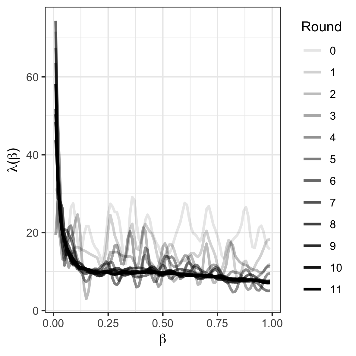
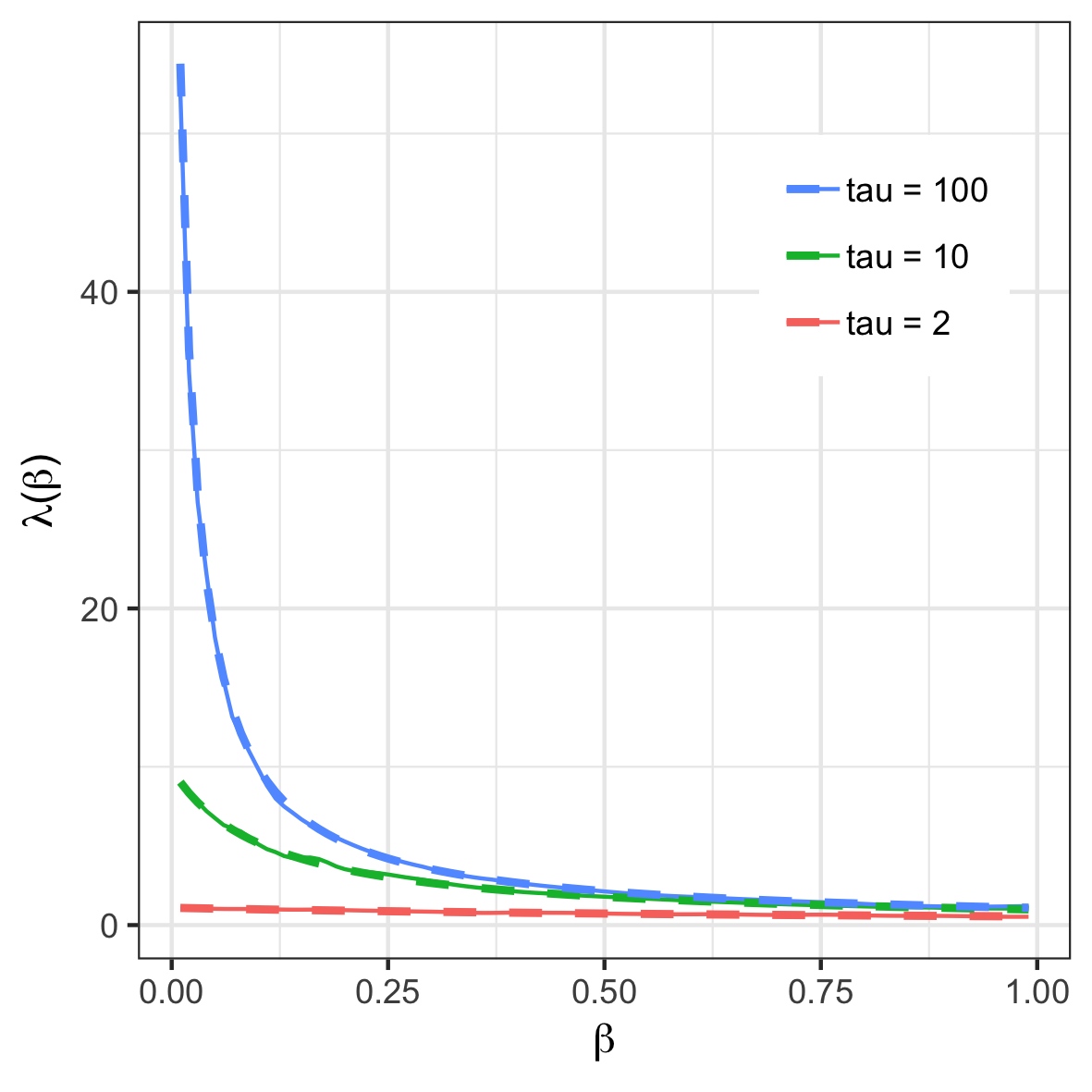
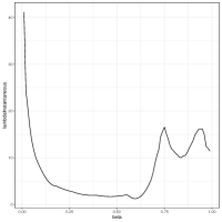
See Figure 7 (center) for examples of estimated λ𝜆\lambda from various models. We define the integral of λ𝜆\lambda by Λ(β)=0βλ(β)dβΛ𝛽superscriptsubscript0𝛽𝜆superscript𝛽differential-dsuperscript𝛽\Lambda(\beta)=\int_{0}^{\beta}\lambda(\beta^{\prime})\mathrm{d}\beta^{\prime} and denote Λ=Λ(1)ΛΛ1\Lambda=\Lambda(1). Extending Proposition 1 in [Predescu et al., 2004] provides the following result.

Theorem 2.

The instantaneous rejection rate λ𝜆\lambda is twice continuously differentiable and is equal to

λ(β)=12𝔼[|V1(β)V2(β)|],𝜆𝛽12𝔼delimited-[]subscriptsuperscript𝑉𝛽1superscriptsubscript𝑉2𝛽\lambda(\beta)=\frac{1}{2}{\mathbb{E}}\left[|V^{(\beta)}_{1}-V_{2}^{(\beta)}|\right], (22)

where V1(β),V2(β)superscriptsubscript𝑉1𝛽superscriptsubscript𝑉2𝛽V_{1}^{(\beta)},V_{2}^{(\beta)} are independent random variables with law identical to the law of V(β)superscript𝑉𝛽V^{(\beta)}. Moreover, we have

r(β,β)𝑟𝛽superscript𝛽\displaystyle r(\beta,\beta^{\prime}) =|Λ(β)Λ(β)|+O(|ββ|3).absentΛsuperscript𝛽Λ𝛽𝑂superscriptsuperscript𝛽𝛽3\displaystyle=|\Lambda(\beta^{\prime})-\Lambda(\beta)|+O(|\beta^{\prime}-\beta|^{3}). (23)

See Appendix C for a proof and general smoothness properties of λ𝜆\lambda. In particular, the existence and smoothness of λ𝜆\lambda is guaranteed by Assumption (A3).

Theorem 2 shows that λ𝜆\lambda encodes up to second order the behaviour of r𝑟r as the annealing parameter difference between the chains goes to 0. When λ(β)𝜆𝛽\lambda(\beta) is high, swaps are much more likely to be rejected, implying λ(β)𝜆𝛽\lambda(\beta) measures the difficulty of local communication for a chain with annealing parameter β𝛽\beta.

Notice that Λ0Λ0\Lambda\geq 0 with equality if and only if λ(β)=0𝜆𝛽0\lambda(\beta)=0 for all β[0,1]𝛽01\beta\in[0,1]. It can be easily verified from (22) that λ=0𝜆0\lambda=0 if and only if V(β)superscript𝑉𝛽V^{(\beta)} is constant π(β)superscript𝜋𝛽\pi^{(\beta)}-a.s. for all β[0,1]𝛽01\beta\in[0,1] which happens precisely when π0=πsubscript𝜋0𝜋\pi_{0}=\pi. So ΛΛ\Lambda defines a natural symmetric divergence measuring the difficulty of communication between π0subscript𝜋0\pi_{0} and π𝜋\pi. In particular, for any schedule 𝒫Nsubscript𝒫𝑁\mathcal{P}_{N}, the sum of the rejection rates is approximately constant and equal to ΛΛ\Lambda as formalized in Corollary 2.

Corollary 2.

For any schedule 𝒫Nsubscript𝒫𝑁\mathcal{P}_{N}, we have

i=1Nr(βi1,βi)=Λ+O(N𝒫N3).superscriptsubscript𝑖1𝑁𝑟subscript𝛽𝑖1subscript𝛽𝑖Λ𝑂𝑁superscriptnormsubscript𝒫𝑁3\displaystyle\sum_{i=1}^{N}r(\beta_{i-1},\beta_{i})=\Lambda+O(N\|\mathcal{P}_{N}\|^{3}). (24)

Motivated by Theorem 2 and Corollary 2 we will henceforth refer to λ𝜆\lambda, ΛΛ\Lambda and Λ()Λ\Lambda(\cdot) as the local, global and cumulative communication barriers respectively.

4.2 Asymptotic analysis of round trip rate

The communication barrier allows us to study the asymptotic performance of PT when the number of parallel chains is large. When N𝑁N increases, the round trip rate for reversible PT decays to 00 while it converges to a positive constant τ¯¯𝜏\bar{\tau} for non-reversible PT as seen in left plot in Figure 3. We formally show this in Theorem 3.

Theorem 3.

As 𝒫N0normsubscript𝒫𝑁0\|\mathcal{P}_{N}\|\to 0 we have:

  1. (a)

    The communication inefficiency satisfies

    ΛE(𝒫N)=Λ+O(𝒫N).Λ𝐸subscript𝒫𝑁Λ𝑂normsubscript𝒫𝑁\displaystyle\Lambda\leq E(\mathcal{P}_{N})=\Lambda+O(\|\mathcal{P}_{N}\|). (25)
  2. (b)

    The round trip rate for reversible PT, τSEOsubscript𝜏𝑆𝐸𝑂\tau_{SEO}, goes to zero:

    τSEO(𝒫N)subscript𝜏SEOsubscript𝒫𝑁\displaystyle\tau_{\mathrm{SEO}}(\mathcal{P}_{N}) 12N+2Λ0.similar-toabsent12𝑁2Λ0\displaystyle\sim\frac{1}{2N+2\Lambda}\longrightarrow 0. (26)
  3. (c)

    The round trip rate for non-reversible PT, τDEOsubscript𝜏𝐷𝐸𝑂\tau_{DEO} satisfies

    τDEO(𝒫N)τ¯=12+2Λ>0,subscript𝜏DEOsubscript𝒫𝑁¯𝜏122Λ0\displaystyle\tau_{\mathrm{DEO}}(\mathcal{P}_{N})\longrightarrow\bar{\tau}=\frac{1}{2+2\Lambda}>0, (27)

    where the converges occurs with rate O(𝒫N)𝑂normsubscript𝒫𝑁O(\|\mathcal{P}_{N}\|).

See Appendix D for a proof.

In general, ΛΛ\Lambda is large when π0subscript𝜋0\pi_{0} deviates significantly from π𝜋\pi. Since ΛΛ\Lambda is problem specific, this identifies a limitation of PT present even in its non-reversible flavour, namely that adding more cores to the task will never be harmful, but does have a diminishing return. The bound (2+2Λ)1superscript22Λ1(2+2\Lambda)^{-1} could indeed be very small for complex problems. Moreover, it is independent of the choice of annealing schedule, hence it cannot be improved by the schedule optimization procedure described in Section 5.

When N𝑁N is fixed, we will see in Section 5.1 that τDEO,τSEOsubscript𝜏DEOsubscript𝜏SEO\tau_{\textrm{DEO}},\tau_{\textrm{SEO}} are both maximized when r(i1,i)=rsuperscript𝑟𝑖1𝑖superscript𝑟r^{(i-1,i)}=r^{*} for all i𝑖i. In this case, E(𝒫N)=N(1r)1r𝐸subscript𝒫𝑁𝑁superscript1superscript𝑟1superscript𝑟E(\mathcal{P}_{N})=N(1-r^{*})^{-1}\leavevmode\nobreak\ r^{*} and one has

N1+NrτDEO(𝒫N)τSEO(𝒫N)=N1+(N1)r1r.𝑁1𝑁superscript𝑟subscript𝜏DEOsubscript𝒫𝑁subscript𝜏SEOsubscript𝒫𝑁𝑁1𝑁1superscript𝑟1superscript𝑟\frac{N}{1+Nr^{\ast}}\leq\frac{\tau_{\textrm{DEO}}(\mathcal{P}_{N})}{\tau_{\textrm{SEO}}(\mathcal{P}_{N})}=\frac{N}{1+(N-1)r^{*}}\leq\frac{1}{r^{*}}. (28)

This implies that for an optimally chosen schedule, non-reversible PT improves the round trip rate over reversible PT by at most a factor of 1/r1superscript𝑟1/r^{*}. Corollary 2 implies NrΛ𝑁superscript𝑟ΛNr^{*}\approx\Lambda, allowing us to quantify the looseness of (28) directly in terms of ΛΛ\Lambda.

1rN1+Nr=1r(11+Nr)1r(11+Λ).1superscript𝑟𝑁1𝑁superscript𝑟1superscript𝑟11𝑁superscript𝑟1superscript𝑟11Λ\frac{1}{r^{*}}-\frac{N}{1+Nr^{*}}=\frac{1}{r^{*}}\left(\frac{1}{1+Nr^{*}}\right)\approx\frac{1}{r^{*}}\left(\frac{1}{1+\Lambda}\right). (29)

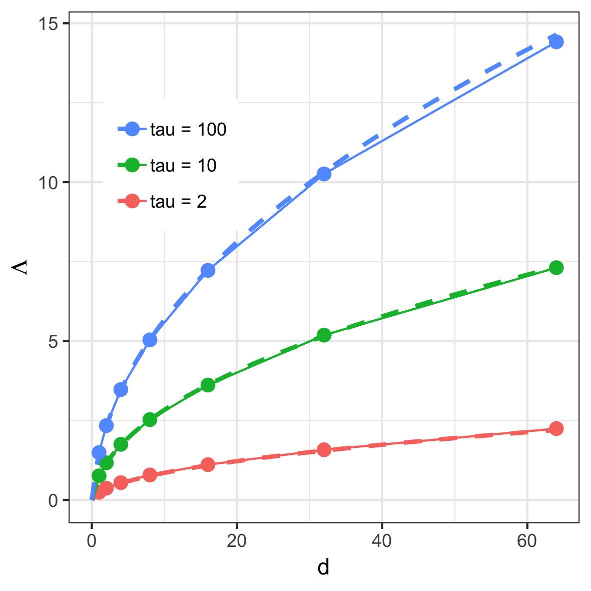
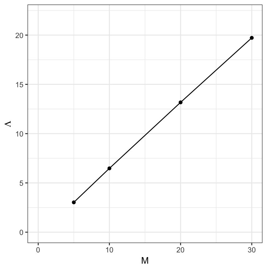
We can also investigate the performance of PT for multi-modal or high-dimensional targets by studying the behaviour of ΛΛ\Lambda. Assuming the target distribution factorizes [Woodard et al., 2009, Atchadé et al., 2011, Roberts and Rosenthal, 2014], we can show that ΛΛ\Lambda is robust to the number of modes and grows at rate O(d)𝑂𝑑O(\sqrt{d}) as the dimension d𝑑d of the target increases. See Appendices E and F for details.

5 Tuning non-reversible PT
Refer to caption
Refer to caption
Refer to caption
Refer to caption
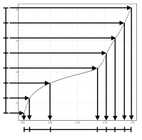
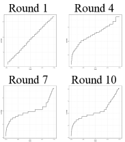
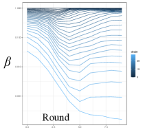
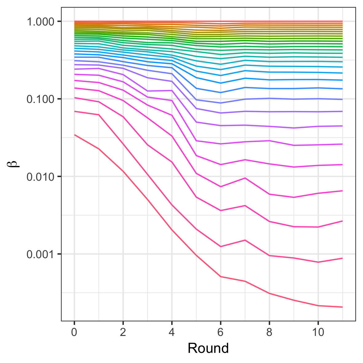
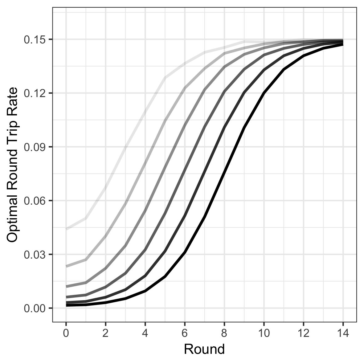
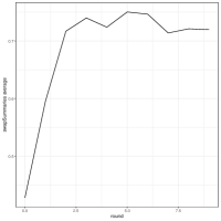
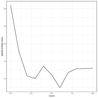
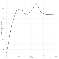
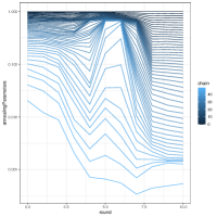
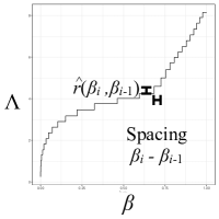
Figure 5: Proposed annealing schedule optimization method: example on the Bayesian mixture model of Section 7. (1) The cumulative barrier Λ()Λ\Lambda(\cdot) is estimated using (32) at each point βksubscript𝛽𝑘\beta_{k} of an initial partition. (2) The cumulative barrier is interpolated using monotonic cubic interpolation, and a new schedule (shown beside the abscissa axis) is obtained by computing the inverse under Λ()Λ\Lambda(\cdot) of a regular grid (shown beside the ordinate). (3) The process 1–2 is repeated iteratively. (4) The sequence of annealing schedules obtained as a function of the round (colours represent different grid points in the schedule).

5.1 Optimal annealing schedule

We first discuss how to optimize the annealing schedule 𝒫Nsubscript𝒫𝑁\mathcal{P}_{N} to maximize τDEOsubscript𝜏DEO\tau_{\textrm{DEO}} when N𝑁N is fixed, which is equivalent to minimizing the schedule inefficiency, E(𝒫N)=i=1Nri/(1ri)𝐸subscript𝒫𝑁superscriptsubscript𝑖1𝑁subscript𝑟𝑖1subscript𝑟𝑖E(\mathcal{P}_{N})=\sum_{i=1}^{N}r_{i}/(1-r_{i}) where ri=r(βi1,βi)subscript𝑟𝑖𝑟subscript𝛽𝑖1subscript𝛽𝑖r_{i}=r(\beta_{i-1},\beta_{i}). To get a tractable approximate characterization of the feasible region of r1,r2,,rNsubscript𝑟1subscript𝑟2subscript𝑟𝑁r_{1},r_{2},\dots,r_{N}, we use Corollary 2, which implies i=1NriΛsuperscriptsubscript𝑖1𝑁subscript𝑟𝑖Λ\sum_{i=1}^{N}r_{i}\approx\Lambda for all schedules 𝒫Nsubscript𝒫𝑁\mathcal{P}_{N}. Therefore assuming 𝒫Nnormsubscript𝒫𝑁\|\mathcal{P}_{N}\| is small enough to ignore the error term, finding the optimal schedule 𝒫Nsuperscriptsubscript𝒫𝑁\mathcal{P}_{N}^{*} is approximately equivalent to minimizing i=1Nri/(1ri)superscriptsubscript𝑖1𝑁subscript𝑟𝑖1subscript𝑟𝑖\sum_{i=1}^{N}r_{i}/(1-r_{i}), subject to the constraint i=1Nri=Λsuperscriptsubscript𝑖1𝑁subscript𝑟𝑖Λ\sum_{i=1}^{N}r_{i}=\Lambda and ri>0subscript𝑟𝑖0r_{i}>0. Using Lagrange multipliers this leads to a solution where the rejection probabilities risuperscriptsubscript𝑟𝑖r_{i}^{*} are constant in i𝑖i, with a shared value denoted by rsuperscript𝑟r^{*}.

Consequently the optimal schedule 𝒫N={β0,,βN}superscriptsubscript𝒫𝑁superscriptsubscript𝛽0superscriptsubscript𝛽𝑁\mathcal{P}_{N}^{*}=\{\beta_{0}^{*},\dots,\beta_{N}^{*}\} satisfies r(βi1,βi)=r𝑟subscriptsuperscript𝛽𝑖1subscriptsuperscript𝛽𝑖superscript𝑟r(\beta^{*}_{i-1},\beta^{*}_{i})=r^{*} for all i𝑖i. Theorem 2 and Corollary 2 imply that rsuperscript𝑟r^{*} must satisfy, rΛ(βi)Λ(βi1)superscript𝑟Λsuperscriptsubscript𝛽𝑖Λsuperscriptsubscript𝛽𝑖1r^{*}\approx\Lambda(\beta_{i}^{*})-\Lambda(\beta_{i-1}^{*}) for all i𝑖i and rΛ/Nsuperscript𝑟Λ𝑁r^{*}\approx\Lambda/N with O(N3)𝑂superscript𝑁3O(N^{-3}) error. By equating these two estimates for rsuperscript𝑟r^{*} and summing from i=0,,k𝑖0𝑘i=0,\dots,k we get

Λ(βk)kNΛ,Λsuperscriptsubscript𝛽𝑘𝑘𝑁Λ\displaystyle\Lambda(\beta_{k}^{*})\approx\frac{k}{N}\Lambda, (30)

with an error of O(N2)𝑂superscript𝑁2O(N^{-2}). If we ignore error terms, (30) implies that βkG(k/N)superscriptsubscript𝛽𝑘𝐺𝑘𝑁\beta_{k}^{*}\approx G(k/N) where G=F1𝐺superscript𝐹1G=F^{-1} and F(β)=Λ(β)/Λ𝐹𝛽Λ𝛽ΛF(\beta)=\Lambda(\beta)/\Lambda (see Figure 5(2)). See Appendix I.4.1 for an example where an analytic result is available, however in general Λ()Λ\Lambda(\cdot) is not known but instead estimated from the MCMC output.

The “equi-acceptance” result in (30) is consistent with other theoretical frameworks and notions of efficiency [Atchadé et al., 2011, Lingenheil et al., 2009, Kofke, 2002, Predescu et al., 2004]. However implementing this equi-acceptance recommendation in practice is non-trivial. Previous work relied on Robbins-Monro schemes [Atchadé et al., 2011, Miasojedow et al., 2013], which introduce sensitive tuning parameters. In contrast, provided Λ()Λ\Lambda(\cdot) can be estimated reliably (which we establish with Algorithm 3 in the next section), (30) provides the basis for a straightforward and effective schedule optimization scheme, described in Algorithm 2.

Algorithm 2 UpdateSchedule(communication barrier Λ()Λ\Lambda(\cdot), schedule size N𝑁N)
1:ΛΛ(1)ΛΛ1\Lambda\leftarrow\Lambda(1)
2:for k𝑘k in 0,1,2,,N012𝑁0,1,2,...,N do
3:     Find βksubscriptsuperscript𝛽𝑘\beta^{*}_{k} such that Λ(βk)=kNΛΛsubscriptsuperscript𝛽𝑘𝑘𝑁Λ\Lambda(\beta^{*}_{k})=\frac{k}{N}\Lambda using e.g. bisection.
4:return 𝒫N=(β0,β1,β2,,βN)superscriptsubscript𝒫𝑁subscriptsuperscript𝛽0subscriptsuperscript𝛽1subscriptsuperscript𝛽2subscriptsuperscript𝛽𝑁\mathcal{P}_{N}^{*}=(\beta^{*}_{0},\beta^{*}_{1},\beta^{*}_{2},\dots,\beta^{*}_{N})

5.2 Estimation of the communication barrier

Assume we have access to a collection of samples (X¯1,X¯2,,X¯n)subscript¯X1subscript¯X2subscript¯X𝑛(\bar{\textbf{X}}_{1},\bar{\textbf{X}}_{2},\dots,\bar{\textbf{X}}_{n}) from a non-reversible PT scheme based on an arbitrary annealing schedule 𝒫Nsubscript𝒫𝑁\mathcal{P}_{N}. These samples may come from a short pilot run, or, as described in the next section, from the previous round of an iterative scheme. For a given schedule 𝒫Nsubscript𝒫𝑁\mathcal{P}_{N}, when the central limit theorem for Markov chains holds, the Monte Carlo estimates for the rejection rates satisfy

r^(i1,i)=1nk=1nα(i1,i)(X¯k)=r(i1,i)+Op(n1/2).superscript^𝑟𝑖1𝑖1𝑛superscriptsubscript𝑘1𝑛superscript𝛼𝑖1𝑖subscript¯X𝑘superscript𝑟𝑖1𝑖subscript𝑂𝑝superscript𝑛12\hat{r}^{(i-1,i)}=\frac{1}{n}\sum_{k=1}^{n}\alpha^{(i-1,i)}(\bar{\textbf{X}}_{k})=r^{(i-1,i)}+O_{p}(n^{-1/2}). (31)

Next, using Theorem 2 we obtain i=1kr(i1,i)=Λ(βk)+O(N𝒫N3)superscriptsubscript𝑖1𝑘superscript𝑟𝑖1𝑖Λsubscript𝛽𝑘𝑂𝑁superscriptnormsubscript𝒫𝑁3\sum_{i=1}^{k}r^{(i-1,i)}=\Lambda(\beta_{k})+O(N\|\mathcal{P}_{N}\|^{3}). This motivates the following approximation for Λ(βk)Λsubscript𝛽𝑘\Lambda(\beta_{k}),

Λ^(βk)=i=1kr^(i1,i),^Λsubscript𝛽𝑘superscriptsubscript𝑖1𝑘superscript^𝑟𝑖1𝑖\hat{\Lambda}(\beta_{k})=\sum_{i=1}^{k}\hat{r}^{(i-1,i)}, (32)

which has an error of order Op(N/n+N𝒫N3)subscript𝑂𝑝𝑁𝑛𝑁superscriptnormsubscript𝒫𝑁3O_{p}(\sqrt{N/n}+N\|\mathcal{P}_{N}\|^{3}) (see Figure 5 (left)).

Given Λ^(β0),,Λ^(βN)^Λsubscript𝛽0^Λsubscript𝛽𝑁\hat{\Lambda}(\beta_{0}),\dots,\hat{\Lambda}(\beta_{N}), we estimate the function Λ(β)Λ𝛽\Lambda(\beta) via interpolation, with the constraint that the interpolated function should be monotone increasing since λ(β)0𝜆𝛽0\lambda(\beta)\geq 0. Specifically, we use the Fritsch-Carlson monotone cubic spline method [Fritsch and Carlson, 1980] and denote the monotone interpolation by Λ^(β)^Λ𝛽\hat{\Lambda}(\beta). While we only use Λ^(β)^Λ𝛽\hat{\Lambda}(\beta) in our schedule optimization procedure, it is still useful to estimate λ(β)𝜆𝛽\lambda(\beta) for visualization purpose. We use the derivative of our interpolation, λ^(β)=Λ^(β)^𝜆𝛽superscript^Λ𝛽\hat{\lambda}(\beta)=\hat{\Lambda}^{\prime}(\beta), which is a piecewise quadratic function.

The ideas described in this section so far are summarized in Algorithm 3, which given rejection statistics collected for a fixed annealing schedule provides an estimate of the communication barrier.

Algorithm 3 CommunicationBarrier(rejection rate {r(i1,i)}superscript𝑟𝑖1𝑖\{r^{(i-1,i)}\}, schedule 𝒫Nsubscript𝒫𝑁\mathcal{P}_{N})
1:For each βi𝒫Nsubscript𝛽𝑖subscript𝒫𝑁\beta_{i}\in\mathcal{P}_{N}, compute Λ^(βi)^Λsubscript𝛽𝑖\hat{\Lambda}(\beta_{i}) \triangleright Equation (32)
2:S{(β0,Λ^(β0)),(β1,Λ^(β1)),,(βN,Λ^(βN))}𝑆subscript𝛽0^Λsubscript𝛽0subscript𝛽1^Λsubscript𝛽1subscript𝛽𝑁^Λsubscript𝛽𝑁S\leftarrow\{(\beta_{0},\hat{\Lambda}(\beta_{0})),(\beta_{1},\hat{\Lambda}(\beta_{1})),\dots,(\beta_{N},\hat{\Lambda}(\beta_{N}))\}
3:Compute a monotone increasing interpolation Λ^()^Λ\hat{\Lambda}(\cdot) of the points S𝑆S \triangleright e.g. using [Fritsch and Carlson, 1980]
4:return Λ^()^Λ\hat{\Lambda}(\cdot)

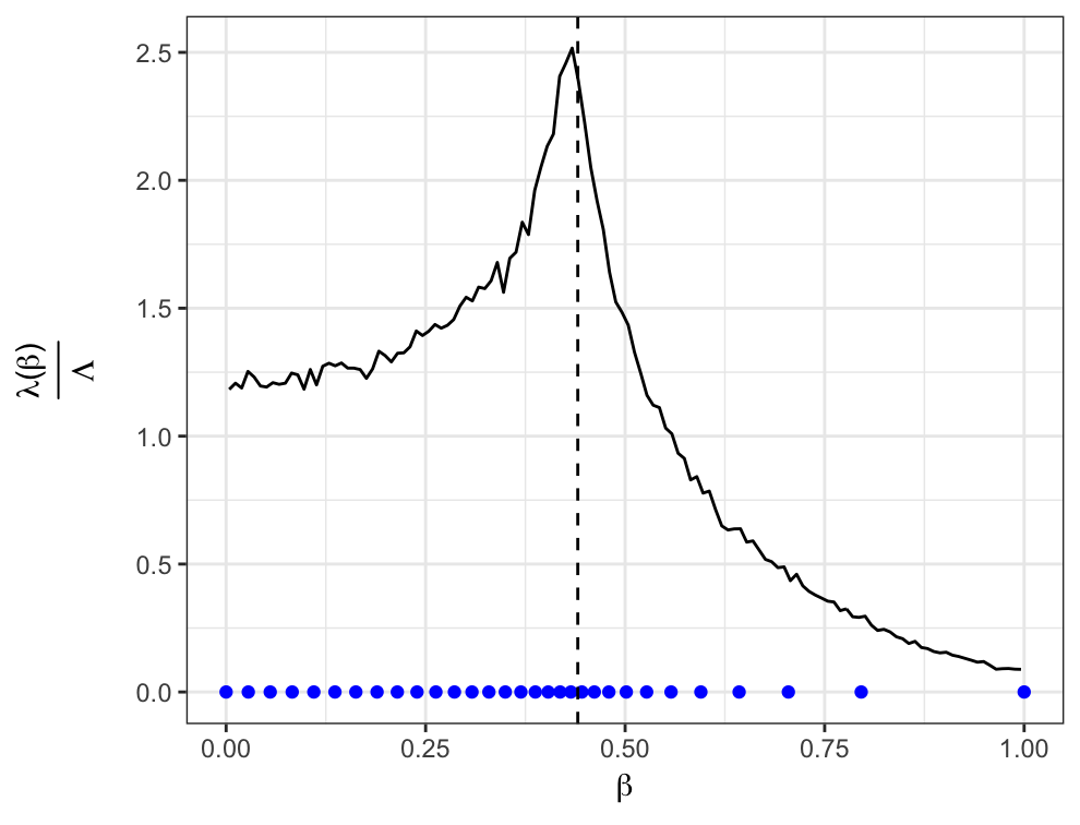
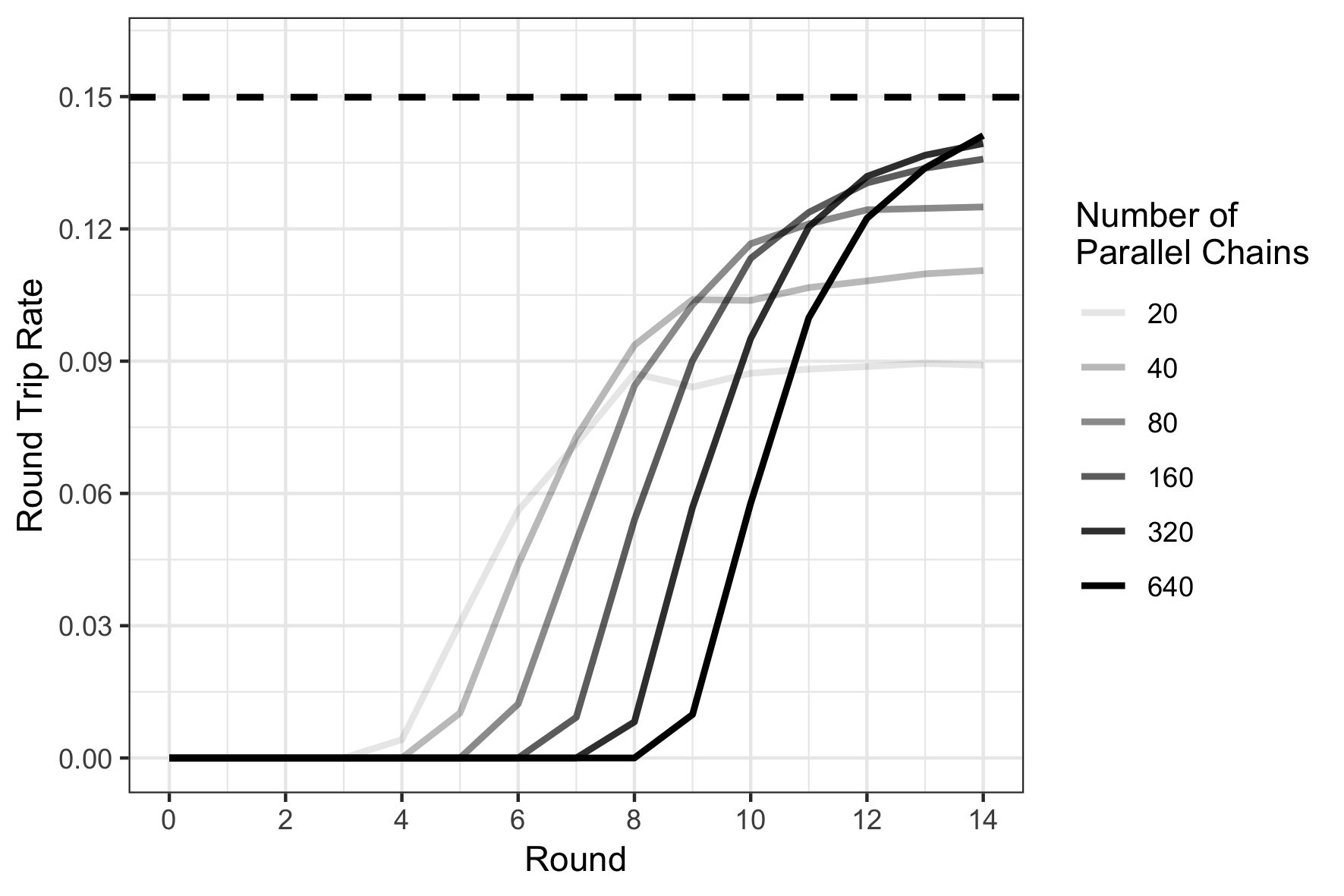
As a byproduct of Algorithm 3 we also obtain a consistent estimator τ^=(2+2Λ^)1^𝜏superscript22^Λ1\hat{\tau}=(2+2\hat{\Lambda})^{-1} for the optimal round trip rate τ¯¯𝜏\bar{\tau}, where Λ^=Λ^(1)^Λ^Λ1\hat{\Lambda}=\hat{\Lambda}(1). We show in Figure 8 an example where (A2) is severely violated, yet λ𝜆\lambda is still reliably estimated. This allows us to compare the empirically observed round trip rate against τ^^𝜏\hat{\tau}, and hence estimate how far an implementation deviates from optimal performance.

5.3 Tuning N𝑁N

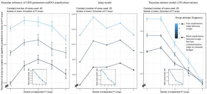
Theorem 3 shows that non-reversible PT does not deteriorate in performance as we increase N𝑁N unlike reversible PT, however the gains in round trip rate eventually become marginal. When N𝑁N is very large we expect to accumulate more round trips by running k>1𝑘1k>1 parallel copies of PT. As we shall see, the large N𝑁N asymptotic is still required however in order to determine the optimal number ksuperscript𝑘k^{*} of PT copies.

Suppose there are k𝑘k copies of PT running in parallel consisting of N+1𝑁1N+1 chains with optimal annealing schedule 𝒫Nsubscript𝒫𝑁\mathcal{P}_{N}. If N¯¯𝑁\bar{N} is the total number of cores available then k𝑘k and N𝑁N satisfy the constraint k(N+1)=N¯𝑘𝑁1¯𝑁k(N+1)=\bar{N}. By Corollary 1 the total round trip rate across all k𝑘k copies of PT is

τ=kτDEO(𝒫N)=N¯2(N+1)(1+E(𝒫N)).𝜏𝑘subscript𝜏DEOsubscript𝒫𝑁¯𝑁2𝑁11𝐸subscript𝒫𝑁\tau=k\ \tau_{\mathrm{DEO}}(\mathcal{P}_{N})=\frac{\bar{N}}{2(N+1)(1+E(\mathcal{P}_{N}))}. (33)

From Section 5.1, the optimal schedule 𝒫Nsuperscriptsubscript𝒫𝑁\mathcal{P}_{N}^{*} has a corresponding swap rejection rate r=Λ/N+O(N3)superscript𝑟Λ𝑁𝑂superscript𝑁3r^{*}=\Lambda/N+O(N^{-3}). Substituting this into (33) we get τ=τΛ(N)+O(N1)𝜏subscript𝜏Λ𝑁𝑂superscript𝑁1\tau=\tau_{\Lambda}(N)+O(N^{-1}), where

τΛ(N)=N¯(1Λ/N)2(N+1)(1Λ/N+Λ).subscript𝜏Λ𝑁¯𝑁1Λ𝑁2𝑁11Λ𝑁Λ\displaystyle\tau_{\Lambda}(N)=\frac{\bar{N}(1-\Lambda/N)}{2(N+1)(1-\Lambda/N+\Lambda)}. (34)

Ignoring error terms, τΛ()subscript𝜏Λ\tau_{\Lambda}(\cdot) is optimized when we run k=N¯/(1+N)superscript𝑘¯𝑁1superscript𝑁k^{*}=\bar{N}/(1+N^{*}) copies of PT with N+1=2Λ+1superscript𝑁12Λ1N^{*}+1=2\Lambda+1 chains to achieve an optimum round trip rate τ=k/(2+4Λ)superscript𝜏superscript𝑘24Λ\tau^{*}=k^{*}/(2+4\Lambda).

Note that when τ𝜏\tau is optimized, we have r1/2superscript𝑟12r^{*}\approx 1/2, which differs from from the 0.770.770.77 optimal rejection rate from the reversible PT literature [Atchadé et al., 2011, Kofke, 2002, Predescu et al., 2004]. In Section 7.2, we show empirically that when the ELE assumption (A2) is severely violated, the recommendation in the present section is turned into a bound, r<1/2superscript𝑟12r^{*}<1/2, as increasing N𝑁N appears to alleviate ELE violations.

5.4 Iterative schedule optimization

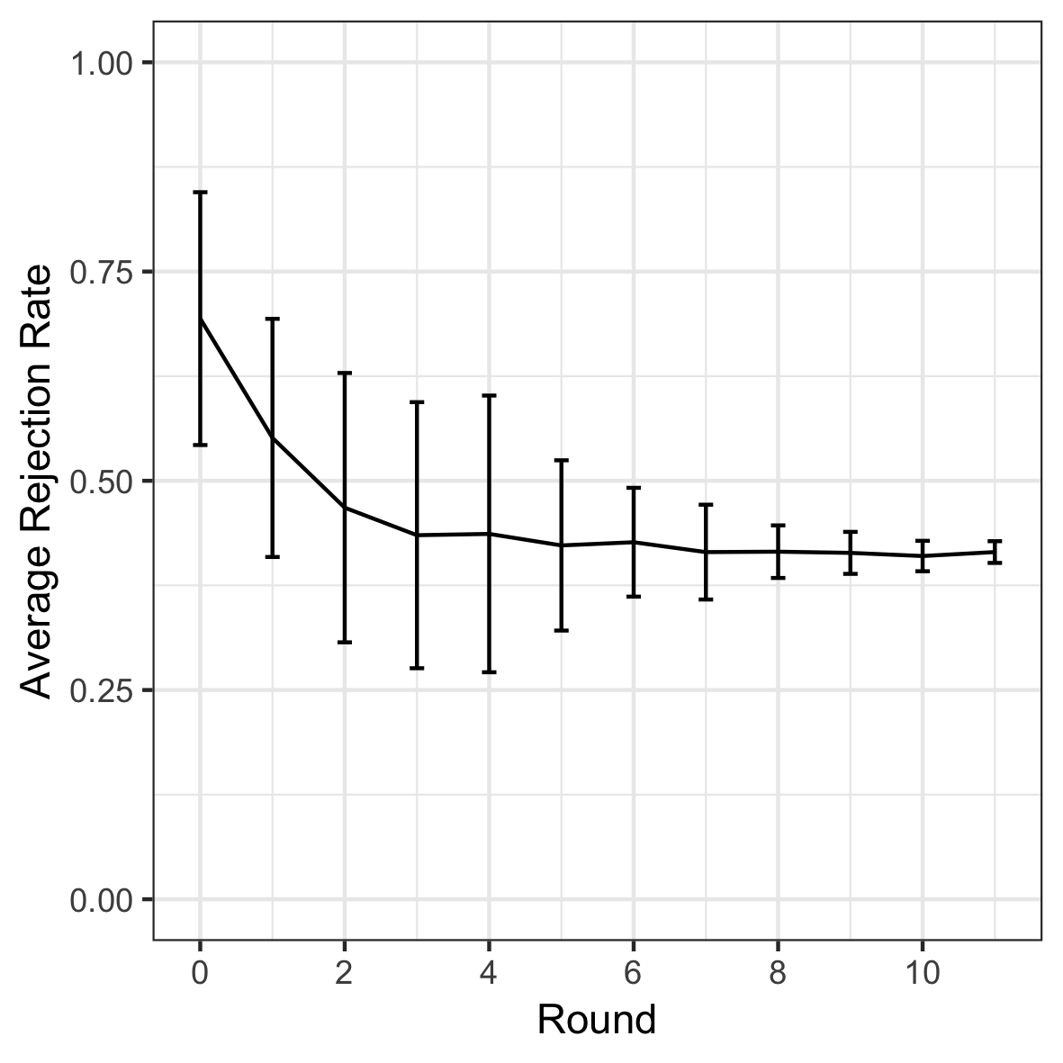
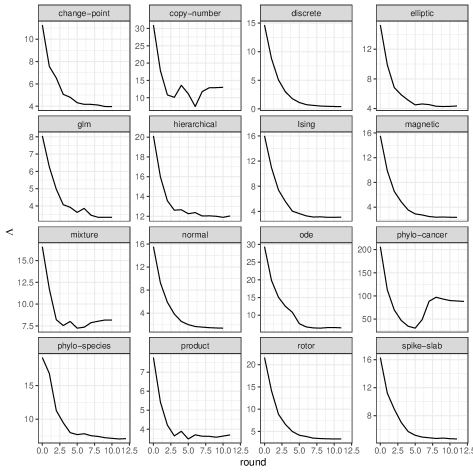
Suppose we have N¯¯𝑁\bar{N} cores available and a computational budget of nscansubscript𝑛scann_{\textrm{scan}} scans of PT, one scan consisting in one application of KPTsuperscriptKPT{\textbf{K}}^{\textrm{PT}}. The first ntunesubscript𝑛tunen_{\textrm{tune}} scans are used to find an accurate estimate of the communication barrier Λ^()^Λ\hat{\Lambda}(\cdot) and the remaining nsample=nscanntunesubscript𝑛samplesubscript𝑛scansubscript𝑛tunen_{\textrm{sample}}=n_{\textrm{scan}}-n_{\textrm{tune}} scans to sample from the target. Algorithm 4 approximates Λ^^Λ\hat{\Lambda} with error Op(N¯/ntune+N¯2)subscript𝑂𝑝¯𝑁subscript𝑛tunesuperscript¯𝑁2O_{p}(\sqrt{\bar{N}/n_{\textrm{tune}}}+\bar{N}^{-2}) by iteratively using Algorithms 2 and 3 for maxRound=log2ntuneabsentsubscript2subscript𝑛tune=\log_{2}n_{\textrm{tune}} rounds until the tuning budget is depleted. Equipped with Λ^()^Λ\hat{\Lambda}(\cdot), we can use the remaining nsamplesubscript𝑛samplen_{\textrm{sample}} scans to run k=N¯/(N+1)superscript𝑘¯𝑁superscript𝑁1k^{*}=\bar{N}/(N^{*}+1) copies of non-reversible PT with N=2Λ^(1)superscript𝑁2^Λ1N^{*}=2\hat{\Lambda}(1) chains with optimal schedule 𝒫Nsuperscriptsubscript𝒫superscript𝑁\mathcal{P}_{N^{*}}^{*} from Algorithm 2. In cases where it is suspected that (A2) may be severely violated (as evidenced for example by a large gap between τ¯¯𝜏\bar{\tau} and the estimated τ𝜏\tau as described in Section 5.2), it may be advantageous to also attempt N=N¯superscript𝑁¯𝑁N^{*}=\bar{N} in line 9 of Algorithm 4. We show empirically in Figure 7 (top) that in a range of synthetic and real world problems our scheme converges using a small number of iterations, in the order of maxRound =10absent10=10. In our experiments we used ntune=nscan/2subscript𝑛tunesubscript𝑛scan2n_{\textrm{tune}}=n_{\textrm{scan}}/2 and discarded the samples from the first ntunesubscript𝑛tunen_{\textrm{tune}} scans as burn-in.

Algorithm 4 NRPT(number of cores N¯¯𝑁\bar{N}, tuning budget ntunesubscript𝑛tunen_{\textrm{tune}}, sampling budget nsamplesubscript𝑛samplen_{\textrm{sample}})
1:𝒫N¯subscript𝒫¯𝑁absent\mathcal{P}_{\bar{N}}\leftarrow initial annealing schedule of size N¯+1¯𝑁1\bar{N}+1 (e.g. uniform)
2:maxRoundlog2(ntune)maxRoundsubscript2subscript𝑛tune\texttt{maxRound}\leftarrow\log_{2}(n_{\textrm{tune}})
3:n1𝑛1n\leftarrow 1 \triangleright Scans per round
4:for round in 1, 2, …, maxRound do
5:     {r(i1,i)}DEO(n,𝒫N¯)superscript𝑟𝑖1𝑖DEO𝑛subscript𝒫¯𝑁\{r^{(i-1,i)}\}\leftarrow\textrm{DEO}(n,\mathcal{P}_{\bar{N}}) \triangleright Algorithm 1
6:     Λ^()^Λabsent\hat{\Lambda}(\cdot)\leftarrowCommunicationBarrier({r(i1,i)},𝒫N¯)superscript𝑟𝑖1𝑖subscript𝒫¯𝑁(\{r^{(i-1,i)}\},\mathcal{P}_{\bar{N}}) \triangleright Algorithm 3
7:     𝒫N¯subscript𝒫¯𝑁absent\mathcal{P}_{\bar{N}}\leftarrowUpdateSchedule(Λ^(),N¯^Λ¯𝑁\hat{\Lambda}(\cdot),\bar{N}) \triangleright Algorithm 2
8:     n2n𝑛2𝑛n\leftarrow 2n \triangleright Rounds use an exponentially increasing number of scans
9:N2Λ^(1)superscript𝑁2^Λ1N^{*}\leftarrow 2\hat{\Lambda}(1) \triangleright See Section 5.3
10:𝒫superscript𝒫absent\mathcal{P}^{*}\leftarrow UpdateSchedule(Λ^(),N^Λsuperscript𝑁\hat{\Lambda}(\cdot),N^{*}) \triangleright Optimal schedule
11:kN¯/(N+1)superscript𝑘¯𝑁superscript𝑁1k^{*}\leftarrow\bar{N}/(N^{*}+1) \triangleright Number of copies of PT
12:for  1,…, ksuperscript𝑘k^{*} do
13:     (x¯1,,x¯nsample)DEO(nsample,𝒫)subscript¯x1subscript¯xsubscript𝑛sampleDEOsubscript𝑛samplesuperscript𝒫(\bar{\textbf{x}}_{1},\dots,\bar{\textbf{x}}_{n_{\textrm{sample}}})\leftarrow\textrm{DEO}(n_{\textrm{sample}},\mathcal{P}^{*})
14:     return (x¯1,,x¯nsample)subscript¯x1subscript¯xsubscript𝑛sample(\bar{\textbf{x}}_{1},\dots,\bar{\textbf{x}}_{n_{\textrm{sample}}})

5.5 Normalizing constant computation

Algorithm 4 can be easily modified to obtain efficient estimators for quantities of the form 01𝔼[f(V(β),β)]dβsuperscriptsubscript01𝔼delimited-[]𝑓superscript𝑉𝛽𝛽differential-d𝛽\int_{0}^{1}{\mathbb{E}}[f(V^{(\beta)},\beta)]\mathrm{d}\beta with an error of Op(N¯/ntune+N¯2)subscript𝑂𝑝¯𝑁subscript𝑛tunesuperscript¯𝑁2O_{p}(\sqrt{\bar{N}/n_{\textrm{tune}}}+\bar{N}^{-2}) for well-behaved functions f𝑓f. Examples of such quantities include log-normalizing constants [Kirkwood, 1935, Gelman and Meng, 1998, Xie et al., 2011], KL-divergence [Dabak and Johnson, 2002], and Fisher-Rao distance [Amari, 2016] between π𝜋\pi and π0subscript𝜋0\pi_{0}.

For example, by taking a Riemann sum in the thermodynamic integration identity [Ogata, 1989], the log-normalizing constant log𝒵(1)𝒵1\log\mathcal{Z}(1) of π𝜋\pi can be approximated using

log𝒵(1)𝒵(0)=01μ(β)dβ=i=1Nμ(βi)(βiβi1)+O(N2),𝒵1𝒵0superscriptsubscript01𝜇𝛽differential-d𝛽superscriptsubscript𝑖1𝑁𝜇subscript𝛽𝑖subscript𝛽𝑖subscript𝛽𝑖1𝑂superscript𝑁2\log\frac{\mathcal{Z}(1)}{\mathcal{Z}(0)}=-\int_{0}^{1}\mu(\beta)\mathrm{d}\beta=-\sum_{i=1}^{N}\mu(\beta_{i})(\beta_{i}-\beta_{i-1})+O(N^{-2}), (35)

where μ(β)=𝔼[V(β)]𝜇𝛽𝔼delimited-[]superscript𝑉𝛽\mu(\beta)={\mathbb{E}}[V^{(\beta)}] and 𝒵(0)𝒵0\mathcal{Z}(0) the normalizing constant of π0subscript𝜋0\pi_{0}. By running DEO with schedule 𝒫Nsubscript𝒫𝑁\mathcal{P}_{N} for n𝑛n scans we substitute a Monte Carlo estimate μ^(βk)^𝜇subscript𝛽𝑘\hat{\mu}(\beta_{k}) for μ(βk)𝜇subscript𝛽𝑘\mu(\beta_{k}) into (35) to get an estimator log(𝒵^(1)/𝒵^(0))^𝒵1^𝒵0\log(\hat{\mathcal{Z}}(1)/\hat{\mathcal{Z}}(0)) with error Op(N/n+N2)subscript𝑂𝑝𝑁𝑛superscript𝑁2O_{p}(\sqrt{N/n}+N^{-2}). See also [Gelman and Meng, 1998, Xie et al., 2011] for closely related normalization constant estimators. Figure 7 (bottom) in Section 7.1 shows how the estimate for log𝒵(1)𝒵1\log\mathcal{Z}(1) evolves with the number of rounds in Algorithm 4 for 16 different models.

6 Scaling limits of index process

The non-reversible communication scheme introduced in [Okabe et al., 2001] was presumably devised on algorithmic grounds (it performs the maximum number of swap attempts in parallel) since no theoretical justification was provided and the non-reversibility of the scheme was not mentioned. The arguments given in [Lingenheil et al., 2009] to explain the superiority of non-reversible communication over various PT algorithms rely on a misleading assumption, namely a diffusive scaling limit for the index process. Figure 1 (see also Figure 15 in the Supplementary Material) suggests that the index process behaves qualitatively differently as N𝑁N increases for reversible and non-reversible PT. The goal of this section is to investigate these differences by identifying some scaling limits. Such limits exist under assumptions (A1)-(A3) specified in Section 3.3 and Section 4.1.

Suppose G:[0,1][0,1]:𝐺0101G:[0,1]\to[0,1] is an increasing differentiable function satisfying G(0)=0𝐺00G(0)=0 and G(1)=1𝐺11G(1)=1. We say that G𝐺G is a schedule generator for 𝒫N={β0,,βN}subscript𝒫𝑁subscript𝛽0subscript𝛽𝑁\mathcal{P}_{N}=\{\beta_{0},\dots,\beta_{N}\} if βi=G(i/N)subscript𝛽𝑖𝐺𝑖𝑁\beta_{i}=G(i/N). We will now assume without loss of generality that the sequence of schedules 𝒫Nsubscript𝒫𝑁\mathcal{P}_{N} are generated by some common G𝐺G. In particular the mean value theorem implies 𝒫N=O(N1)normsubscript𝒫𝑁𝑂superscript𝑁1\|\mathcal{P}_{N}\|=O(N^{-1}) as N𝑁N\to\infty. This is not a strict requirement as most annealing schedules commonly used fall within this framework: the uniform schedule 𝒫Nuniform={0,1/N,,1}superscriptsubscript𝒫𝑁uniform01𝑁1\mathcal{P}_{N}^{\text{uniform}}=\{0,1/N,\dots,1\} is generated by G(w)=w𝐺𝑤𝑤G(w)=w, the optimal schedule 𝒫N={β0,,βN}superscriptsubscript𝒫𝑁superscriptsubscript𝛽0superscriptsubscript𝛽𝑁\mathcal{P}_{N}^{*}=\{\beta_{0}^{*},\dots,\beta_{N}^{*}\} derived in Section 5.1 is approximately generated by G(w)=F1(w)𝐺𝑤superscript𝐹1𝑤G(w)=F^{-1}(w), where F(β)=Λ(β)/Λ𝐹𝛽Λ𝛽ΛF(\beta)=\Lambda(\beta)/\Lambda. If π0(x)π(x)γproportional-tosubscript𝜋0𝑥𝜋superscript𝑥𝛾\pi_{0}(x)\propto\pi(x)^{\gamma} for some γ(0,1)𝛾01\gamma\in(0,1), and L(x)π(x)1γproportional-to𝐿𝑥𝜋superscript𝑥1𝛾L(x)\propto\pi(x)^{1-\gamma} then G(w)=γ1wγ1γ𝐺𝑤superscript𝛾1𝑤𝛾1𝛾G(w)=\frac{\gamma^{1-w}-\gamma}{1-\gamma} corresponds to the geometric schedule commonly used by practitioners. In contrast, we show in Figure 20 examples of schedule generators G𝐺G corresponding to estimated optimal 𝒫Nsuperscriptsubscript𝒫𝑁\mathcal{P}_{N}^{*} from various models. Figure 20 shows that in real world inference scenarios, the optimal G𝐺G often qualitatively differs from the simple geometric schedule.

Suppose (In,εn)subscript𝐼𝑛subscript𝜀𝑛(I_{n},\varepsilon_{n}) is the index process for an annealing schedule 𝒫Nsubscript𝒫𝑁\mathcal{P}_{N} generated by G𝐺G. To establish a scaling limit for (In,εn)subscript𝐼𝑛subscript𝜀𝑛(I_{n},\varepsilon_{n}), it will be convenient to work in a continuous time setting. To do this, we suppose the times that PT iterations occur are distributed according to a Poisson process {M()}𝑀\{M(\cdot)\} with mean μNsubscript𝜇𝑁\mu_{N}. The number M(t)𝑀𝑡M(t) of PT iterations that occur by time t0𝑡0t\geq 0 thus satisfies M(t)Poisson(μNt)similar-to𝑀𝑡Poissonsubscript𝜇𝑁𝑡M(t)\sim\mathrm{Poisson}(\mu_{N}t). We define the scaled index process by ZN(t)=(WN(t),εN(t))superscript𝑍𝑁𝑡superscript𝑊𝑁𝑡superscript𝜀𝑁𝑡Z^{N}(t)=(W^{N}(t),\varepsilon^{N}(t)) where WN(t)=IM(t)/Nsuperscript𝑊𝑁𝑡subscript𝐼𝑀𝑡𝑁W^{N}(t)=I_{M(t)}/N and εN(t)=εM(t)superscript𝜀𝑁𝑡subscript𝜀𝑀𝑡\varepsilon^{N}(t)=\varepsilon_{M(t)}.

Define the piecewise-deterministic Markov process (PDMP) [Davis, 1993] Z(t)=(W(t),ε(t))𝑍𝑡𝑊𝑡𝜀𝑡Z(t)=(W(t),\varepsilon(t)) on [0,1]×{1,1}0111[0,1]\times\{-1,1\} as follows: W(t)𝑊𝑡W(t) moves in [0,1]01[0,1] with velocity ε(t)𝜀𝑡\varepsilon(t) and the sign of ε(t)𝜀𝑡\varepsilon(t) is reversed at an inhomogeneous rate λ(G(W(t))G(W(t))\lambda(G(W(t))G^{\prime}(W(t)) or when W(t)𝑊𝑡W(t) hits a boundary; see [Bierkens et al., 2018] for a discussion of PDMP on restricted domains. The process Z𝑍Z corresponds to an inhomogeneous persistent random walk with reflective boundary conditions; see [Masoliver et al., 1992] for a description of the Fokker-Plank equation and first passage times. As the optimal schedule is generated by G=F1𝐺superscript𝐹1G=F^{-1} for F(β)=Λ(β)/Λ𝐹𝛽Λ𝛽ΛF(\beta)=\Lambda(\beta)/\Lambda, we have λ(G(w))G(w)=Λ𝜆𝐺𝑤superscript𝐺𝑤Λ\lambda(G(w))G^{\prime}(w)=\Lambda for all w[0,1]𝑤01w\in[0,1], so ε(t)𝜀𝑡\varepsilon(t) changes sign at a constant rate ΛΛ\Lambda. See Figure 13 for sample trajectories of Z𝑍Z for different values of ΛΛ\Lambda. The main result of this section is the following theorem.

Theorem 4.

Suppose 𝒫Nsubscript𝒫𝑁\mathcal{P}_{N} is family of schedules generated by G𝐺G, then

  1. (a)

    For reversible PT if μN=N2subscript𝜇𝑁superscript𝑁2\mu_{N}=N^{2} and if WN(0)superscript𝑊𝑁0W^{N}(0) converges weakly to W(0)𝑊0W(0) then WNsuperscript𝑊𝑁W^{N} converges weakly to a diffusion W𝑊W with initial condition W(0)𝑊0W(0), where W𝑊W is a Brownian motion on [0,1]01[0,1] with reflective boundary conditions. The process W𝑊W admits Unif([0,1])Unif01\mathrm{Unif}([0,1]) as stationary distribution.

  2. (b)

    For non-reversible PT if μN=Nsubscript𝜇𝑁𝑁\mu_{N}=N and if ZN(0)superscript𝑍𝑁0Z^{N}(0) converges weakly to Z(0)𝑍0Z(0), then ZNsuperscript𝑍𝑁Z^{N} converges weakly to the PDMP Z𝑍Z with initial condition Z(0)𝑍0Z(0). The process Z𝑍Z admits Unif([0,1]×{1,1})Unif0111\mathrm{Unif}([0,1]\times\{-1,1\}) as stationary distribution.

See Appendix G for a detailed construction of the scaled index process via their infinitesimal generators, and the proof of Theorem 4.

Theorem 4 implies for reversible PT that, if we speed time by a factor of N2superscript𝑁2N^{2}, then the index process scales to a diffusion W𝑊W independent of the choice of π0,πsubscript𝜋0𝜋\pi_{0},\pi and of the schedule. This is in contrast to non-reversible PT where, if we speed time by a factor of N𝑁N, the index process converges to a PDMP Z𝑍Z depending on π0,πsubscript𝜋0𝜋\pi_{0},\pi through λ𝜆\lambda and the schedule through G𝐺G.

7 Examples

7.1 Empirical behaviour of the schedule optimization method

We applied the proposed NRPT algorithm to 16 models from the statistics and physics literature to demonstrate its versatility. The models include 9 Bayesian models ranging from simple standard models such as generalized linear models and Bayesian mixtures, to complex ones such as cancer copy-number calling, ODE parameter estimation, spike-and-slab classification and two types of phylogenetic models. This is complemented by three models from statistical mechanics and four artificial models. The datasets considered include eight real datasets spanning diverse data-types and size, e.g. state-of-the-art measurements such as whole-genome single-cell sequencing data (494 individual cells from two types of cancer, triple negative breast cancer and high-grade serous ovarian [Dorri et al., 2020]) and mRNA transfection time series [Leonhardt et al., 2014], as well as more conventional ones such as mtDNA data and various feature selection/classification datasets. See Figure 6 and references therein for details. See also Appendix I for more information on the models and additional experimental results. All models and algorithms are implemented in the Blang modelling language [Bouchard-Côté et al., 2019].

In each of the 16 models and for each round of Algorithm 4 (line 4), we computed the mean swap acceptance probability across all neighbour chains. We then summarized these means across chains using a box plot. The equi-acceptance objective function of Section 5.1 can be visually understood as collapsing this box plot into a single point. We show in Figure 7 (top) the progression of these swap acceptance probabilities. In all examples considered, equi-acceptance is well approximated within 10 rounds.

Within the range of models considered, we observed a diversity of local barriers λ𝜆\lambda estimated by Algorithm 4 (Figure 7 (middle)). Most statistical models exhibit a high but narrow peak in the neighbourhood of the reference (β=0𝛽0\beta=0). However, a subset of models including statistical models (mixture, ode, phylo-cancer, spike-slab) and physics models (Ising, magnetic, rotor) exhibit additional peaks away from β=0𝛽0\beta=0. See Figure 20 in Appendix J.1 for the corresponding schedule generators G𝐺G and global barriers ΛΛ\Lambda.

Model (and dataset when applicable) n𝑛n d𝑑d Λ^^Λ\hat{\Lambda} N𝑁N
Change point detection (text message data, [Davidson-Pilon, 2015]) 747474 333 4.04.04.0 202020
Copy number inference (whole genome ovarian cancer data, Section 7.5) 6 20662066\;206 303030 13.013.013.0 505050
Discrete multimodal distribution (Appendix I.4.3) N/A 333 0.40.40.4 303030
Weakly identifiable elliptic curve (Appendix I.4) N/A 222 4.44.44.4 303030
General Linear Model (GLM) (Challenger O-ring dataset, [Dalal et al., 1989]) 232323 222 3.33.33.3 151515
Bayesian hierarchical model (historical rocket failure data, Appendix I.4) 5 66756675\;667 369369369 12.012.012.0 303030
Ising model (Appendix I.4.2) N/A 252525 3.13.13.1 303030
Ising model with magnetic field (Appendix I.4.2) N/A 252525 2.32.32.3 303030
Bayesian mixture model (Section I.4.4) 300300300 305305305 8.28.28.2 303030
Bayesian mixture model (subset of 150 datapoints) 150150150 155155155 5.55.55.5 202020
Isotropic normal distribution N/A 555 1.41.41.4 303030
ODE parameters (mRNA data, [Leonhardt et al., 2014]) 525252 555 6.46.46.4 505050
Phylogenetic inference (single cell breast cancer data, [Dorri et al., 2020]) 192 763192763192\;763 192 765192765192\;765 888888 300300300
Phylogenetic species tree inference (mtDNA, [Hayasaka et al., 1988]) 249249249 10 3951039510\;395 7.17.17.1 303030
Unidentifiable product parameterization (Appendix I.4) 100 000100000100\;000 222 3.73.73.7 151515
Rotor (XY) model, [Hsieh et al., 2013] N/A 252525 3.33.33.3 404040
Spike-and-slab classification (RMS Titanic passengers data [Hind, 2019]) 200200200 191919 4.74.74.7 303030
Figure 6: Summary of models used in the experiments, with the number of observations n𝑛n (when applicable), the number of latent random variables d𝑑d, estimated Λ^^Λ\hat{\Lambda}, and the default number of chains used. An abbreviation for each is shown in italic.
Refer to caption
Refer to caption
Refer to caption
Figure 7: Empirical behaviour of NRPT on 16 models. Top: distribution of acceptance rates observed at each round of Algorithm 4. Middle: estimates of the local communication barrier λ^^𝜆\hat{\lambda}. Bottom: progression of the log normalization constant estimates (Section 5.5) produced during each NRPT adaptation round.

7.2 Robustness to ELE violation

To investigate empirically whether the NRPT methodology is robust to the violation of the ELE assumption, we ran NRPT with a range of values for nexplsubscript𝑛expln_{\textrm{expl}} on the models shown in Figure 8. Let dvarsubscript𝑑vard_{\text{var}} denote the number of variables in each model. We run experiments with nexpl=0subscript𝑛expl0n_{\textrm{expl}}=0, (1/2)dvar12subscript𝑑var(1/2)d_{\text{var}}, dvarsubscript𝑑vard_{\text{var}}, 2dvar2subscript𝑑var2d_{\text{var}}, 4dvar4subscript𝑑var4d_{\text{var}}, …, 32dvar32subscript𝑑var32d_{\text{var}} (the only exception is the reference chain (β=0𝛽0\beta=0), where we always use nexpl=1subscript𝑛expl1n_{\textrm{expl}}=1 since we can get exact samples from π0subscript𝜋0\pi_{0}). The key quantity used by the NRPT algorithm for schedule optimization is the communication barrier λ𝜆\lambda. The results shown in Figure 8 demonstrate that in all models considered the function λ𝜆\lambda is reliably estimated even when ELE is severely violated, provided nexpl>0subscript𝑛expl0n_{\textrm{expl}}>0. Similarly, since the estimates of ΛΛ\Lambda and τ¯¯𝜏\bar{\tau} are derived from λ𝜆\lambda, these quantities can be accurately estimated even when ELE is severely violated (see Figure 19 in Appendix I.4.2). The results shown in Figure 3 support that increasing nexplsubscript𝑛expln_{\textrm{expl}} reduces the difference between the theoretical and observed round trip rate. Moreover, Figure 3 also demonstrate a second strategy to alleviate ELE violation, which is to increase N𝑁N while fixing nexplsubscript𝑛expln_{\textrm{expl}}.

In the next experiment shown in Figure 9, we compare the two mechanisms available for alleviating ELE violation, namely increasing N𝑁N and increasing nexplsubscript𝑛expln_{\textrm{expl}}. First consider the black line in Figure 9 showing the regime where ELE is best approximated in these experiments. This is in close agreement with the theoretical guidelines developed in Section 5.3. At the same time, the light blue lines in Figure 9 show that in situations where the local exploration kernel is not easy to parallelize, it can be advantageous to decrease nexplsubscript𝑛expln_{\textrm{expl}} and to compensate with a number of chains N𝑁N higher than 2Λ2Λ2\Lambda, leading to an average swap rejection rate r<1/2𝑟12r<1/2.

Refer to caption
Figure 8: Estimate λ^^𝜆\hat{\lambda} of the local communication barrier λ𝜆\lambda for different values of nexpl0subscript𝑛expl0n_{\textrm{expl}}\geq 0 and different models (refer to Figure 6 for model descriptions). The estimates are consistent as long as nexpl>0subscript𝑛expl0n_{\textrm{expl}}>0, even when assumption (A2) is severely violated. Refer to Section 7.2 for experiment details.
Refer to caption
Figure 9: Trade-off between number of chains N𝑁N, number of independent PT algorithms, k𝑘k, and the frequency at which swaps are attempted (1/nexplproportional-toabsent1subscript𝑛expl\propto 1/n_{\textrm{expl}}). Each model uses a constant number of cores and set N+1=N¯/k𝑁1¯𝑁𝑘N+1=\bar{N}/k chains per independent PT algorithm. Insets: swap acceptance probability for each k𝑘k. The results in the black lines (where ELE is best approximated) agree with the theory of Section 5.3. For the ODE model, Λ6.4Λ6.4\Lambda\approx 6.4, N12.8superscript𝑁12.8N^{*}\approx 12.8 in agreement with k=3superscript𝑘3k^{*}=3 observed. For the Ising model, Λ3.1Λ3.1\Lambda\approx 3.1, N6.2superscript𝑁6.2N^{*}\approx 6.2 in agreement with k=4superscript𝑘4k^{*}=4 observed. For the Bayesian mixture model, Λ5.5Λ5.5\Lambda\approx 5.5, N11superscript𝑁11N^{*}\approx 11, in agreement with k=2superscript𝑘2k^{*}=2 observed. These results also show that in the context of local exploration moves that are not easily parallelized, it is better to use higher swap attempt frequencies (light blue lines) which achieve their optima at N>2Λ𝑁2ΛN>2\Lambda and average swap rejection rate r<1/2𝑟12r<1/2.

7.3 Comparison with other parallel tempering schemes

We benchmarked the empirical running time of Algorithm 4 compared to previous adaptive PT methods [Atchadé et al., 2011, Miasojedow et al., 2013]. The methods we considered are: (1) the stochastic optimization adaptive method for reversible schemes proposed in [Atchadé et al., 2011]; (2), a second stochastic optimization scheme, which still selects the optimal number of chains using the 23%percent2323\% rule but uses an improved update scheme from [Miasojedow et al., 2013], refer to Appendix I.3 for details; (3) our non reversible schedule optimization scheme (NRPT); and finally, (4) our scheme, combined with a better initialization based on a preliminary execution of a sequential Monte Carlo algorithm (more precisely, based on a “sequential change of measure,” labelled SCM, as described in [Del Moral et al., 2006]), we use this to investigate the effect on the violation of the stationarity assumption, and for fairness, we use this sophisticated initialization method for all the methods except (3). We benchmarked the methods on four models: (a) a 369-dimensional hierarchical model applied to a dataset of rocket launch failure/success indicator variables [McDowell, 2019]; (b) a 19-dimensional Spike-and-Slab variable selection model applied to the RMS Titanic Passenger Manifest dataset [Hind, 2019]; (c) A 25-dimensional Ising model from Section I.4.2 (M=5𝑀5M=5); (d) a 9-dimensional model for an end-point conditioned Wright-Fisher stochastic differential equation (see, e.g., [Tataru et al., 2017]).

We provide the same number of cores and parallelized all the methods to the greatest extent possible. We refer the reader to Appendix I for implementation details, experimental setup, and detailed description of the models and datasets used.

In Figure 10, each dot summarized in the box plots represents the ESS per total wall clock time in seconds including schedule optimization time for the marginal of one of the model variables. The results show that schedule optimization is more efficient with our proposed non-reversible scheme, with a speed-up in the 10–100 range for the four models considered. The results also suggest that sequential Monte Carlo based initialization may not have a large impact on the performance of our method. See Figure 21 in Appendix J.2 for other summary statistics from this benchmark.
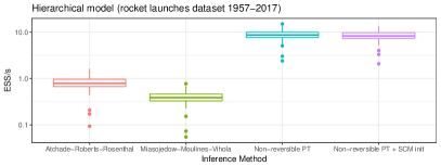
Refer to caption
Refer to caption
Refer to caption
Refer to caption
Figure 10: Effective Sample Size (ESS) per second (ordinate, in log scale) for four PT methods (abscissa). The four facets show results for the four models described in Section 7.3.

7.4 Mixture models

Refer to caption
Figure 11: Mixture model example: eight approximations of the posterior distributions, showing for each approximation two of the 155 latent random variables, namely the two component mixtures’ mean parameters. Since the two latent random variables are exchangeable a posteriori (by label switching), the true marginal posterior distributions are identical for the two random variables. Amongst the approximation methods, multimodality is only captured by our algorithm (NRPT, 1.508min) and by a state-of-the-art sequential Monte Carlo combined with several rounds of rejuvenation (SCM-100, 5.064min). The benchmark is conservative in that all competing methods use a computational budget (in terms of both parallelism and wall clock time) greater or equal than NRPT.

Bayesian analysis of mixture models can give rise to a label-switching symmetry, leading to a multimodal posterior distribution (see Appendix I.4.4). In Figure 11 we compare the following inference methods on a label-switching posterior distribution: our proposed algorithm (NRPT), an MCMC run based on a single chain (i.e. the exploration kernel alone), the stochastic optimization method of Miasojedow-Moulines-Vihola (MMV), DEO but optimized using MMV (MMV-DEO), Annealed Importance Sampling (AIS) [Neal, 2001], and a sequential Monte Carlo based on a sequence of annealed distributions [Del Moral et al., 2006] (labelled SCM as before). For both SCM and AIS, we use the adaptive scheme of [Zhou et al., 2016] (see Figure 24 in Appendix J.3 for diagnostics of the SCM adaptation). The number of iterations are set so that the method with the smallest wall clock time is our proposed algorithm (NRPT: 1.508min, MMV: 2.019min, MMV-DEO:1.665min, AIS: 1.887min, SCM: 1.778min–5.064min). For all methods, timing includes the time spent to perform schedule optimization.

Amongst MCMC methods, only NRPT correctly captures the multimodality of the target distribution. This is confirmed by the trace plots of the three MCMC methods, shown in Figure 25 in Appendix J.3. MMV automatically selected N=8𝑁8N=8 by targeting an swap acceptance probability of 23%percent2323\%. Post-adaptation, the swap acceptance probability was 27%percent2727\%. For NRPT we use N=30𝑁30N=30 but to avoid penalizing MMV for a lack of parallelism, we limited all methods to use no more than 888 threads. After schedule optimization, NRPT estimates the global communication barrier to a value of Λ^8^Λ8\hat{\Lambda}\approx 8, and the average swap acceptance probability was 72%percent7272\% (see Figure 26 in Appendix J.3 for more NRPT diagnostics).

7.5 Multimodality arising from single cell, whole genome copy number inference

In this section we describe an application to copy number inference in which multimodality arises from the unknown ploidy of a cancer cell. The likelihood of this model is based on a hidden Markov model over n=6 206𝑛6206n=6\,206 observations, and after analytic marginalization of the corresponding 6 20662066\,206 hidden states, the multimodal sampling problem is defined over d=30𝑑30d=30 remaining latent variables. The model is described in Appendix I.4.5, in this section we summarize the results concerning the performance of the algorithms.

We compare the quality of posterior approximations from four samplers on the High-Grade Serous Ovarian cancer dataset from [Dorri et al., 2020]. The four methods compared are: the stochastic optimization adaptive PT method MMV (adaptation selected 777 chains, average post-adaptation swap acceptance, 28.7%percent28.728.7\%), DEO but optimized using MMV (MMV-DEO, adaptation selected 111111 chains, average post-adaptation swap acceptance, 26.9%percent26.926.9\%) our proposed algorithm algorithm (NRPT with 25 and 50 chains, average post-optimization swap acceptance of respectively 48.8%percent48.848.8\% and 73.5%percent73.573.5\%), and inference based on a single MCMC chain. As in Section 7.4, to avoid overly penalizing MMV for a lack of parallelism, we limited all methods to use no more than 888 threads, hence obtaining the following wall clock running times including schedule optimization when applicable: MMV, 15.91h; MMV+DEO, 14.33h; 25 chains NRPT, 8.809h; 50 chains NRPT, 15.35h; 1 chain MCMC, 2.91h. The running time of MMV was dominated by adaptation (88% of the wall clock time), and is higher than the schedule optimization time used by NRPT (67%).

Refer to Figure 12 for a comparison of the trace plots between all three methods. Since the experimental protocol provides only proportionality between read counts and copy number, not absolute expected read count for a given copy number, the likelihood does not distinguish between a given copy number profile, and another one obtained by genome duplication of the same profile (refer to Appendix I.4.5 for details). The prior favours the former, but when local copy number events occur after the genome duplication it may be possible to detect recently evolved genome duplication. Challenging multimodality arises when these subsequent events involve only small regions. In such case, the tension between the prior distribution favouring low ploidy and the noisy observation favouring higher ploidy creates a multimodal posterior distribution. We use data from one such cell in the following experiments to illustrate a realistic multimodal inference problem.

The multimodality of the posterior distribution was successfully captured by NRPT but not by a single-chain MCMC nor by the stochastic optimization method MMV (Figure 12). MMV failed to achieve any round trip because the learnt schedule is highly suboptimal: while the mean swap acceptance probability across chains is 28.7%percent28.728.7\%, the minimum across chains is nearly zero due to the noise in the optimization procedure. The difficulty of exploring this particular multimodal target is compounded by the fact that the state space of each chromosome’s copy number is random, being upper-bounded by random variables mcsubscript𝑚𝑐m_{c} corresponding to each chromosome c𝑐c. So in order to perform a jump doubling the cell’s ploidy the sampler has to increase a large number of discrete variables mcsubscript𝑚𝑐m_{c} simultaneously. This is reflected in the posterior distribution of the model variables denoted mcsubscript𝑚𝑐m_{c}, shown in Figure 28 in Appendix J.4. Hence the local exploration kernel, which in this example samples the variables mcsubscript𝑚𝑐m_{c} one at the time, is insufficient to jump mode, and only excursions through the prior can achieve mode jumping, via a regeneration based on sampling from the prior at β=0𝛽0\beta=0.

NRPT used 50 chains, estimated Λ^=13^Λ13\hat{\Lambda}=13 (see Figure 30 in Appendix J.4), and converged quickly in this large scale example, performing drastic changes in the annealing schedule in the first 8 rounds then relatively little changes in rounds 8 through the final tenth round (Figure 30).

Comparing the performance of the two NRPT variants, we estimated a round trip rate of 9×1049superscript1049\times 10^{-4} for 25-chain, and 6×1036superscript1036\times 10^{-3} for 50-chain. Notice the increase being more than a factor two supports the use of large N𝑁N for exploration of complex multimodal posterior distributions. Neither MMV nor MMV-DEO achieved any round trips in the post-burn-in iterations.

Refer to caption
Figure 12: Trace plots for the copy number inference problem. Each facet shows a post burn-in trace plot for one of the discrete random variables mcsubscript𝑚𝑐m_{c}. Facet rows are indexed by chromosomes. Facet columns are indexed by MCMC approximation methods. The trace plots show that only NRPT frequently jumps between the two modes. MMV and the exploration kernel alone do not achieve any jump, due to the required concerted changes in a large number of discrete variables. See Figure 29 in Appendix J.4 for a larger version.

8 Discussion

We have established that under the ELE assumption, non-reversible PT dominates reversible PT in terms of round trip rates for any choice of N𝑁N and annealing schedule 𝒫Nsubscript𝒫𝑁\mathcal{P}_{N} (Corollary 1). Moreover we have characterized the optimal round trip rate in terms of the communication barrier ΛΛ\Lambda, which we have used to identify an intrinsic limitation of both reversible and non-reversible PT (Section 4.2), and to design a novel schedule optimization method (Section 5). We have shown that this schedule optimization method outperforms previous schedule optimizers in a range of numerical simulations, and we are already aware of other research groups that have successfully applied our methodology in astronomy [Akiyama et al., 2021, Issaoun et al., 2021] and engineering [Langmore et al., 2021].

By combining (28) with the estimate r1/2superscript𝑟12r^{*}\approx 1/2 derived from (34), our theoretical results indicate a 1/r21superscript𝑟21/r^{*}\approx 2-fold increase in the round trip rate of DEO compared to SEO in an idealized setting where the ELE assumption holds and the schedule, including the number of chains, is well-tuned. The efficiency gains can be more pronounced during schedule optimization, in the course of which the number of chains can be initially larger than the optimal number of chains specified in Section 5.3 as a consequence of Theorem 3. Moreover, our experimental results show that previous methods to tune PT schedules can be fragile. Compared to these previous methods, we have observed speedups of one to two orders of magnitude thanks to our schedule optimization method.

References

  • [Akiyama et al., 2021] Akiyama, K. et al. (2021). First M87 Event Horizon Telescope Results. VII. Polarization of the Ring. The Astrophysical Journal Letters, 910:12–59.
  • [Altekar et al., 2004] Altekar, G., Dwarkadas, S., Huelsenbeck, J. P., and Ronquist, F. (2004). Parallel Metropolis coupled Markov chain Monte Carlo for Bayesian phylogenetic inference. Bioinformatics, 20(3):407–415.
  • [Amari, 2016] Amari, S.-i. (2016). Information Geometry and Its Applications, volume 194. Springer.
  • [Atchadé et al., 2011] Atchadé, Y. F., Roberts, G. O., and Rosenthal, J. S. (2011). Towards optimal scaling of Metropolis-coupled Markov chain Monte Carlo. Statistics and Computing, 21(4):555–568.
  • [Ballnus et al., 2017] Ballnus, B., Hug, S., Hatz, K., Görlitz, L., Hasenauer, J., and Theis, F. J. (2017). Comprehensive benchmarking of Markov chain Monte Carlo methods for dynamical systems. BMC Systems Biology, 11(1):63.
  • [Baxter, 2007] Baxter, R. J. (2007). Exactly Solved Models in Statistical Mechanics. Dover books on Physics. Dover Publications.
  • [Beroukhim et al., 2010] Beroukhim, R. et al. (2010). The landscape of somatic copy-number alteration across human cancers. Nature, 463(7283):899–905.
  • [Bierkens et al., 2018] Bierkens, J., Bouchard-Côté, A., Doucet, A., Duncan, A. B., Fearnhead, P., Lienart, T., Roberts, G. O., and Vollmer, S. J. (2018). Piecewise deterministic Markov processes for scalable Monte Carlo on restricted domains. Statistics & Probability Letters, 136:148–154.
  • [Billingsley, 2013] Billingsley, P. (2013). Convergence of Probability Measures. John Wiley & Sons.
  • [Böttcher et al., 2013] Böttcher, B., Schilling, R., and Wang, J. (2013). Lévy matters. III, volume 2099 of Lecture Notes in Mathematics.
  • [Bouchard-Côté et al., 2019] Bouchard-Côté, A., Chern, K., Cubranic, D., Hosseini, S., Hume, J., Lepur, M., Ouyang, Z., and Sgarbi, G. (2019). Blang: Bayesian declarative modelling of arbitrary data structures. arXiv:1912.10396.
  • [Chandra et al., 2019] Chandra, R., Jain, K., Deo, R. V., and Cripps, S. (2019). Langevin-gradient parallel tempering for Bayesian neural learning. Neurocomputing, 359:315–326.
  • [Chen et al., 1999] Chen, F., Lovász, L., and Pak, I. (1999). Lifting Markov chains to speed up mixing. In Proceedings of the 31st Annual ACM Symposium on Theory of Computing, pages 275–281. ACM.
  • [Cho et al., 2010] Cho, K., Raiko, T., and Ilin, A. (2010). Parallel tempering is efficient for learning restricted Boltzmann machines. In Neural Networks (IJCNN), The 2010 International Joint Conference on, pages 1–8. IEEE.
  • [Dabak and Johnson, 2002] Dabak, A. G. and Johnson, D. H. (2002). Relations between Kullback–Leibler distance and Fisher information. Technical report, Rice University.
  • [Dalal et al., 1989] Dalal, S. R., Fowlkes, E. B., and Hoadley, B. (1989). Risk Analysis of the Space Shuttle: Pre-Challenger Prediction of Failure. Journal of the American Statistical Association, 84(408):945–957.
  • [Davidson-Pilon, 2015] Davidson-Pilon, C. (2015). Bayesian Methods for Hackers: Probabilistic Programming and Bayesian Inference. Addison-Wesley Professional, New York, 1st edition.
  • [Davis, 1993] Davis, M. H. (1993). Markov Models & Optimization. Chapman and Hall.
  • [Del Moral et al., 2006] Del Moral, P., Doucet, A., and Jasra, A. (2006). Sequential Monte Carlo samplers. Journal of the Royal Statistical Society. Series B (Statistical Methodology), 68(3):411–436.
  • [Desjardins et al., 2014] Desjardins, G., Luo, H., Courville, A., and Bengio, Y. (2014). Deep tempering. arXiv preprint arXiv:1410.0123.
  • [Diaconis et al., 2000] Diaconis, P., Holmes, S., and Neal, R. M. (2000). Analysis of a nonreversible Markov chain sampler. The Annals of Applied Probability, 10(3):726–752.
  • [Diaz et al., 2020] Diaz, A., Argüelles, C., Collin, G., Conrad, J., and Shaevitz, M. (2020). Where are we with light sterile neutrinos? Physics Reports, 884:1–59.
  • [Dorri et al., 2020] Dorri, F., Salehi, S., Chern, K., Funnell, T., Williams, M., Lai, D., Andronescu, M., Campbell, K. R., McPherson, A., Aparicio, S., Roth, A., Shah, S. P., and Bouchard-Côté, A. (2020). Efficient Bayesian inference of phylogenetic trees from large scale, low-depth genome-wide single-cell data. bioR Xiv 2020.05.06.058180.
  • [Ethier and Kurtz, 2009] Ethier, S. N. and Kurtz, T. G. (2009). Markov Processes: Characterization and Convergence, volume 282. John Wiley & Sons.
  • [Fang et al., 2014] Fang, Y., Feng, S., Tam, K.-M., Yun, Z., Moreno, J., Ramanujam, J., and Jarrell, M. (2014). Parallel tempering simulation of the three-dimensional Edwards-Anderson model with compact asynchronous multispin coding on GPU. Computer Physics Communications, 185(10):2467–2478.
  • [Friesen, 2015] Friesen, J. (2015). Java Threads and the Concurrency Utilities. Apress, Berkeley, CA, USA, 1st edition.
  • [Fritsch and Carlson, 1980] Fritsch, F. and Carlson, R. (1980). Monotone piecewise cubic interpolation. SIAM Journal on Numerical Analysis, 17(2):238–246.
  • [Gelman and Meng, 1998] Gelman, A. and Meng, X.-L. (1998). Simulating normalizing constants: From importance sampling to bridge sampling to path sampling. Statistical Science, pages 163–185.
  • [Geyer, 1991] Geyer, C. J. (1991). Markov chain Monte Carlo maximum likelihood. Interface Proceedings.
  • [Hayasaka et al., 1988] Hayasaka, K., Gojobori, T., and Horai, S. (1988). Molecular phylogeny and evolution of primate mitochondrial DNA. Molecular Biology and Evolution, 5(6):626–644. Publisher: Oxford Academic.
  • [Hind, 2019] Hind, P. (2019). RMS Titanic passenger dataset. data retrieved from https://tinyurl.com/y55c8kc7.
  • [Hsieh et al., 2013] Hsieh, Y.-D., Kao, Y.-J., and Sandvik, A. W. (2013). Finite-size scaling method for the Berezinskii-Kosterlitz-Thouless transition. Journal of Statistical Mechanics: Theory and Experiment, 2013(09):P09001.
  • [Hukushima and Nemoto, 1996] Hukushima, K. and Nemoto, K. (1996). Exchange Monte Carlo method and application to spin glass simulations. Journal of the Physical Society of Japan, 65(6):1604–1608.
  • [Issaoun et al., 2021] Issaoun, S. et al. (2021). Persistent non-Gaussian structure in the image of Sagittarius A* at 86 GHz. arXiv:2104.07610.
  • [Kallenberg, 2002] Kallenberg, O. (2002). Foundations of Modern Probability. Springer, 2nd edition.
  • [Kamberaj, 2020] Kamberaj, H. (2020). Molecular Dynamics Simulations in Statistical Physics: Theory and Applications. Springer.
  • [Katzgraber et al., 2006] Katzgraber, H. G., Trebst, S., Huse, D. A., and Troyer, M. (2006). Feedback-optimized parallel tempering Monte Carlo. Journal of Statistical Mechanics: Theory and Experiment, 2006(03):P03018.
  • [Kirkwood, 1935] Kirkwood, J. G. (1935). Statistical mechanics of fluid mixtures. The Journal of Chemical Physics, 3(5):300–313.
  • [Kofke, 2002] Kofke, D. A. (2002). On the acceptance probability of replica-exchange Monte Carlo trials. The Journal of Chemical Physics, 117(15):6911–6914.
  • [Kone and Kofke, 2005] Kone, A. and Kofke, D. A. (2005). Selection of temperature intervals for parallel-tempering simulations. The Journal of Chemical Physics, 122(20):206101.
  • [Łacki and Miasojedow, 2016] Łacki, M. K. and Miasojedow, B. (2016). State-dependent swap strategies and automatic reduction of number of temperatures in adaptive parallel tempering algorithm. Statistics and Computing, 26(5):951–964.
  • [Lai et al., 2020] Lai, D., Ha, G., and Shah, S. (2020). HMMcopy: Copy number prediction with correction for GC and mappability bias for HTS data.
  • [Langmore et al., 2021] Langmore, I., Dikovsky, M., Geraedts, S., Norgaard, P., and von Behren, R. (2021). Hamiltonian Monte Carlo in Inverse Problems; Ill-Conditioning and Multi-Modality. arXiv:2103.07515.
  • [Leiserson et al., 2012] Leiserson, C. E., Schardl, T. B., and Sukha, J. (2012). Deterministic parallel random-number generation for dynamic-multithreading platforms. MIT web domain.
  • [Lelièvre et al., 2010] Lelièvre, T., Stoltz, G., and Rousset, M. (2010). Free Energy Computations: A Mathematical Perspective. World Scientific.
  • [Leonhardt et al., 2014] Leonhardt, C., Schwake, G., Stögbauer, T. R., Rappl, S., Kuhr, J.-T., Ligon, T. S., and Rädler, J. O. (2014). Single-cell mRNA transfection studies: delivery, kinetics and statistics by numbers. Nanomedicine: Nanotechnology, Biology, and Medicine, 10(4):679–688.
  • [Lingenheil et al., 2009] Lingenheil, M., Denschlag, R., Mathias, G., and Tavan, P. (2009). Efficiency of exchange schemes in replica exchange. Chemical Physics Letters, 478(1-3):80–84.
  • [Lunn et al., 2000] Lunn, D. J., Thomas, A., Best, N., and Spiegelhalter, D. (2000). WinBUGS - a Bayesian modelling framework: Concepts, structure, and extensibility. Statistics and Computing, 10(4):325–337.
  • [Masoliver et al., 1992] Masoliver, J., Porra, J. M., and Weiss, G. H. (1992). Solutions of the telegrapher’s equation in the presence of traps. Physical Review A, 45(4):2222.
  • [McDowell, 2019] McDowell, J. (2019). Launch logs. data retrieved from https://tinyurl.com/y5veq9yf.
  • [Miasojedow et al., 2013] Miasojedow, B., Moulines, E., and Vihola, M. (2013). An adaptive parallel tempering algorithm. Journal of Computational and Graphical Statistics, 22(3):649–664.
  • [Mingas and Bouganis, 2012] Mingas, G. and Bouganis, C.-S. (2012). Parallel tempering MCMC acceleration using reconfigurable hardware. In Choy, O. C. S., Cheung, R. C. C., Athanas, P., and Sano, K., editors, Reconfigurable Computing: Architectures, Tools and Applications, Lecture Notes in Computer Science, pages 227–238. Springer Berlin Heidelberg.
  • [Müller and Bouckaert, 2020] Müller, N. F. and Bouckaert, R. R. (2020). Adaptive parallel tempering for BEAST 2. bioRxiv:10.1101/603514.
  • [Nadler and Hansmann, 2007] Nadler, W. and Hansmann, U. H. E. (2007). Dynamics and optimal number of replicas in parallel tempering simulations. Physical Review E, 76(6):065701.
  • [Neal, 2001] Neal, R. M. (2001). Annealed importance sampling. Statistics and Computing, 11(2):125–139.
  • [Neal, 2003] Neal, R. M. (2003). Slice sampling. The Annals of Statistics, 31(3):705–767.
  • [Ogata, 1989] Ogata, Y. (1989). A Monte Carlo method for high dimensional integration. Numerische Mathematik, 55:137–157.
  • [Okabe et al., 2001] Okabe, T., Kawata, M., Okamoto, Y., and Mikami, M. (2001). Replica-exchange Monte Carlo method for the isobaric–isothermal ensemble. Chemical Physics Letters, 335(5-6):435–439.
  • [Predescu et al., 2004] Predescu, C., Predescu, M., and Ciobanu, C. V. (2004). The incomplete beta function law for parallel tempering sampling of classical canonical systems. The Journal of Chemical Physics, 120(9):4119–4128.
  • [Rathore et al., 2005] Rathore, N., Chopra, M., and de Pablo, J. J. (2005). Optimal allocation of replicas in parallel tempering simulations. The Journal of Chemical Physics, 122(2):024111.
  • [Roberts and Rosenthal, 2014] Roberts, G. O. and Rosenthal, J. S. (2014). Minimising MCMC variance via diffusion limits, with an application to simulated tempering. The Annals of Applied Probability, 24(1):131–149.
  • [Sakai and Hukushima, 2016] Sakai, Y. and Hukushima, K. (2016). Irreversible simulated tempering. Journal of the Physical Society of Japan, 85(10):104002.
  • [Saranen and Seikkala, 1988] Saranen, J. and Seikkala, S. (1988). Solution of a nonlinear two-point boundary value problem with Neumann-type boundary data. Journal of Mathematical Analysis and Applications, 135(2):691–701.
  • [Steele and Lea, 2013] Steele, G. and Lea, D. (2013). Splittable random application programming interface. https://docs.oracle.com/javase/8/docs/api/java/util/SplittableRandom.html. [Online; accessed 6-May-2019].
  • [Swendsen and Wang, 1986] Swendsen, R. H. and Wang, J.-S. (1986). Replica Monte Carlo simulation of spin-glasses. Physical Review Letters, 57(21):2607.
  • [Tataru et al., 2017] Tataru, P., Simonsen, M., Bataillon, T., and Hobolth, A. (2017). Statistical inference in the Wright-Fisher model using allele frequency data. Systematic Biology, 66(1):e30–e46.
  • [Turitsyn et al., 2011] Turitsyn, K. S., Chertkov, M., and Vucelja, M. (2011). Irreversible Monte Carlo algorithms for efficient sampling. Physica D: Nonlinear Phenomena, 240(4-5):410–414.
  • [Vucelja, 2016] Vucelja, M. (2016). Lifting: a nonreversible Markov chain Monte Carlo algorithm. American Journal of Physics, 84(12):958–968.
  • [Woodard et al., 2009] Woodard, D. B., Schmidler, S. C., Huber, M., et al. (2009). Conditions for rapid mixing of parallel and simulated tempering on multimodal distributions. The Annals of Applied Probability, 19(2):617–640.
  • [Wu, 2017] Wu, F. (2017). Irreversible Parallel Tempering and an Application to a Bayesian Nonparametric Latent Feature Model. Master’s thesis, Oxford University.
  • [Xie et al., 2011] Xie, W., Lewis, P. O., Fan, Y., Kuo, L., and Chen, M.-H. (2011). Improving marginal likelihood estimation for Bayesian phylogenetic model selection. Systematic Biology, 60(2):150–160.
  • [Zahn et al., 2017] Zahn, H., Steif, A., Laks, E., Eirew, P., VanInsberghe, M., Shah, S. P., Aparicio, S., and Hansen, C. L. (2017). Scalable whole-genome single-cell library preparation without preamplification. Nature Methods, 14(2):167–173.
  • [Zhou et al., 2016] Zhou, Y., Johansen, A. M., and Aston, J. A. (2016). Toward automatic model comparison: An adaptive sequential Monte Carlo approach. Journal of Computational and Graphical Statistics, 25(3):701–726.
  • [Zhu et al., 2020] Zhu, P., Bouchard-Côté, A., and Campbell, T. (2020). Slice Sampling for General Completely Random Measures. In Proceedings of the 36th Conference on Uncertainty in Artificial Intelligence (UAI), volume 36.

Supplementary material

Appendix A Markov kernel for the index process

For SEO, initialize (I0,ε0)=(i,ε)subscript𝐼0subscript𝜀0𝑖𝜀(I_{0},\varepsilon_{0})=(i,\varepsilon). We then define the Markov transition kernel, (In+1,εn+1)|(In,εn)PSEO((In,εn),)similar-toconditionalsubscript𝐼𝑛1subscript𝜀𝑛1subscript𝐼𝑛subscript𝜀𝑛superscript𝑃SEOsubscript𝐼𝑛subscript𝜀𝑛(I_{n+1},\varepsilon_{n+1})|(I_{n},\varepsilon_{n})\sim P^{\mathrm{SEO}}((I_{n},\varepsilon_{n}),\cdot) in two steps. In the first step, simulate

In+1|(In,εn)=(i,ε){(i+ε)N0 with probability s(i,i+ε),i otherwise,conditionalsubscript𝐼𝑛1subscript𝐼𝑛subscript𝜀𝑛𝑖𝜀similar-tocases𝑖𝜀𝑁0 with probability superscript𝑠𝑖𝑖𝜀𝑖 otherwise,I_{n+1}|(I_{n},\varepsilon_{n})=(i,\varepsilon)\sim\begin{cases}(i+\varepsilon)\wedge N\vee 0&\text{ with probability }s^{(i,i+\varepsilon)},\\ i&\text{ otherwise,}\end{cases} (36)

where the expression “N0𝑁0\wedge N\vee 0” enforces the annealing parameter boundaries. In the second step, independently sample εn+1Unif{1,+1}similar-tosubscript𝜀𝑛1Unif11\varepsilon_{n+1}\sim\text{Unif}\{-1,+1\}.

Similarly for DEO, initialize (I0,ε0)=(i0,ε0)subscript𝐼0subscript𝜀0subscript𝑖0subscript𝜀0(I_{0},\varepsilon_{0})=(i_{0},\varepsilon_{0}). Analogous to the SEO construction, we define (In+1,εn+1)|(In,εn)PDEO((In,εn),)similar-toconditionalsubscript𝐼𝑛1subscript𝜀𝑛1subscript𝐼𝑛subscript𝜀𝑛superscript𝑃DEOsubscript𝐼𝑛subscript𝜀𝑛(I_{n+1},\varepsilon_{n+1})|(I_{n},\varepsilon_{n})\sim P^{\mathrm{DEO}}((I_{n},\varepsilon_{n}),\cdot) in two steps. We first update In+1|(In,εn)=(i,ε)conditionalsubscript𝐼𝑛1subscript𝐼𝑛subscript𝜀𝑛𝑖𝜀I_{n+1}|(I_{n},\varepsilon_{n})=(i,\varepsilon) as in (36), but apply the deterministic update in the second step,

εn+1={ε if In+1=i+ε,ε otherwise.subscript𝜀𝑛1cases𝜀 if subscript𝐼𝑛1𝑖𝜀𝜀 otherwise.\varepsilon_{n+1}=\begin{cases}\varepsilon&\text{ if }I_{n+1}=i+\varepsilon,\\ -\varepsilon&\text{ otherwise.}\end{cases} (37)

Appendix B Proof of Theorem 1

To simplify notation for the rest of the proof, let Tsubscript𝑇T_{\uparrow} and Tsubscript𝑇T_{\downarrow} be the hitting times to the target and reference defined by,

T=min{n:(In,εn)=(N,1)},T=min{n:(In,εn)=(0,1)}.formulae-sequencesubscript𝑇:𝑛subscript𝐼𝑛subscript𝜀𝑛𝑁1subscript𝑇:𝑛subscript𝐼𝑛subscript𝜀𝑛01\displaystyle T_{\uparrow}=\min\{n:(I_{n},\varepsilon_{n})=(N,1)\},\;\;\;\ T_{\downarrow}=\min\{n:(I_{n},\varepsilon_{n})=(0,-1)\}. (38)

We will also denote

si=s(i1,i),ri=r(i1,i).formulae-sequencesubscript𝑠𝑖superscript𝑠𝑖1𝑖subscript𝑟𝑖superscript𝑟𝑖1𝑖\displaystyle s_{i}=s^{(i-1,i)},\qquad r_{i}=r^{(i-1,i)}. (39)
  1. (a)

    If we define ai=𝔼SEO(T|I0=i)superscriptsubscript𝑎𝑖subscript𝔼SEOconditionalsubscript𝑇subscript𝐼0𝑖a_{\bullet}^{i}={\mathbb{E}}_{\mathrm{SEO}}(T_{\bullet}|I_{0}=i) for i=0,,N𝑖0𝑁i=0,\dots,N and {,}\bullet\in\{\uparrow,\downarrow\}, then we have

    𝔼SEO(T)=a0+aN.subscript𝔼SEO𝑇superscriptsubscript𝑎0superscriptsubscript𝑎𝑁\displaystyle{\mathbb{E}}_{\mathrm{SEO}}(T)=a_{\uparrow}^{0}+a_{\downarrow}^{N}. (40)

    By the Markov property, for i=1,,N1𝑖1𝑁1i=1,\dots,N-1, aisuperscriptsubscript𝑎𝑖a_{\bullet}^{i} satisfies the recursion

    ai=12si+1(ai+1+1)+12si(ai1+1)+12(ri+1+ri)(ai+1).superscriptsubscript𝑎𝑖12subscript𝑠𝑖1subscriptsuperscript𝑎𝑖1112subscript𝑠𝑖subscriptsuperscript𝑎𝑖1112subscript𝑟𝑖1subscript𝑟𝑖subscriptsuperscript𝑎𝑖1\displaystyle a_{\bullet}^{i}=\frac{1}{2}s_{i+1}(a^{i+1}_{\bullet}+1)+\frac{1}{2}s_{i}(a^{i-1}_{\bullet}+1)+\frac{1}{2}(r_{i+1}+r_{i})(a^{i}_{\bullet}+1). (41)

    For i=1,,N𝑖1𝑁i=1,\dots,N, we substitute in bi=aiai1superscriptsubscript𝑏𝑖superscriptsubscript𝑎𝑖superscriptsubscript𝑎𝑖1b_{\bullet}^{i}=a_{\bullet}^{i}-a_{\bullet}^{i-1} into (41). After simplification, bisubscriptsuperscript𝑏𝑖b^{i}_{\bullet} satisfies the following recursive relation

    2=si+1bi+1sibi.2subscript𝑠𝑖1subscriptsuperscript𝑏𝑖1subscript𝑠𝑖subscriptsuperscript𝑏𝑖\displaystyle-2=s_{i+1}b^{i+1}_{\bullet}-s_{i}b^{i}_{\bullet}. (42)

    The solutions to (42) are

    sibisubscript𝑠𝑖subscriptsuperscript𝑏𝑖\displaystyle s_{i}b^{i}_{\bullet} =s1b12(i1),absentsubscript𝑠1subscriptsuperscript𝑏12𝑖1\displaystyle=s_{1}b^{1}_{\bullet}-2(i-1), (43)

    or equivalently

    sibisubscript𝑠𝑖subscriptsuperscript𝑏𝑖\displaystyle s_{i}b^{i}_{\bullet} =sNbN+2(Ni).absentsubscript𝑠𝑁subscriptsuperscript𝑏𝑁2𝑁𝑖\displaystyle=s_{N}b^{N}_{\bullet}+2(N-i). (44)

    We now deal with the case of \uparrow and \downarrow separately.

    1. (a)

      To determine a0superscriptsubscript𝑎0a_{\uparrow}^{0}, we note that if I0=0subscript𝐼00I_{0}=0 then I1=1subscript𝐼11I_{1}=1 with probability 12s112subscript𝑠1\frac{1}{2}s_{1} and I1=0subscript𝐼10I_{1}=0 otherwise. So a0superscriptsubscript𝑎0a_{\uparrow}^{0} satisfies

      a0=12s1(a1+1)+(112s1)(a0+1),subscriptsuperscript𝑎012subscript𝑠1subscriptsuperscript𝑎11112subscript𝑠1subscriptsuperscript𝑎01\displaystyle a^{0}_{\uparrow}=\frac{1}{2}s_{1}(a^{1}_{\uparrow}+1)+\left(1-\frac{1}{2}s_{1}\right)(a^{0}_{\uparrow}+1), (45)

      or equivalently

      s1b1=2.subscript𝑠1subscriptsuperscript𝑏12\displaystyle s_{1}b^{1}_{\uparrow}=-2. (46)

      Substituting this into (43) implies sibi=2isubscript𝑠𝑖subscriptsuperscript𝑏𝑖2𝑖s_{i}b^{i}_{\uparrow}=-2i. By summing bi=aiai1subscriptsuperscript𝑏𝑖subscriptsuperscript𝑎𝑖subscriptsuperscript𝑎𝑖1b^{i}_{\uparrow}=a^{i}_{\uparrow}-a^{i-1}_{\uparrow} from i=1,,N𝑖1𝑁i=1,\dots,N and, noting aN=0subscriptsuperscript𝑎𝑁0a^{N}_{\uparrow}=0, we get

      a0=i=1N2isi.subscriptsuperscript𝑎0superscriptsubscript𝑖1𝑁2𝑖subscript𝑠𝑖\displaystyle a^{0}_{\uparrow}=\sum_{i=1}^{N}\frac{2i}{s_{i}}. (47)
    2. (b)

      Similarly to determine aNsuperscriptsubscript𝑎𝑁a_{\downarrow}^{N} we note that if I0=Nsubscript𝐼0𝑁I_{0}=N then I1=N1subscript𝐼1𝑁1I_{1}=N-1 with probability 12sN12subscript𝑠𝑁\frac{1}{2}s_{N} and I1=Nsubscript𝐼1𝑁I_{1}=N otherwise. So aNsuperscriptsubscript𝑎𝑁a_{\downarrow}^{N} satisfies

      aN=12sN(aN1+1)+(112sN)(aN+1),subscriptsuperscript𝑎𝑁12subscript𝑠𝑁subscriptsuperscript𝑎𝑁11112subscript𝑠𝑁subscriptsuperscript𝑎𝑁1\displaystyle a^{N}_{\downarrow}=\frac{1}{2}s_{N}(a^{N-1}_{\downarrow}+1)+\left(1-\frac{1}{2}s_{N}\right)(a^{N}_{\downarrow}+1), (48)

      or equivalently

      sNbN=2.subscript𝑠𝑁subscriptsuperscript𝑏𝑁2\displaystyle s_{N}b^{N}_{\downarrow}=2. (49)

      Substituting this into (44) implies sibi=2+2(Ni)subscript𝑠𝑖subscriptsuperscript𝑏𝑖22𝑁𝑖s_{i}b^{i}_{\downarrow}=2+2(N-i). By summing bi=aiai1subscriptsuperscript𝑏𝑖subscriptsuperscript𝑎𝑖subscriptsuperscript𝑎𝑖1b^{i}_{\downarrow}=a^{i}_{\downarrow}-a^{i-1}_{\downarrow} from i=1,,N𝑖1𝑁i=1,\dots,N and, noting a0=0subscriptsuperscript𝑎00a^{0}_{\downarrow}=0, we get

      aN=i=1N2(Ni)+2si.subscriptsuperscript𝑎𝑁superscriptsubscript𝑖1𝑁2𝑁𝑖2subscript𝑠𝑖\displaystyle a^{N}_{\downarrow}=\sum_{i=1}^{N}\frac{2(N-i)+2}{s_{i}}. (50)

    Substituting in (47) and (50) into (40), it follows that

    𝔼SEO(T)subscript𝔼SEO𝑇\displaystyle{\mathbb{E}}_{\mathrm{SEO}}(T) =i=1N2isi+i=1N2(Ni)+2siabsentsuperscriptsubscript𝑖1𝑁2𝑖subscript𝑠𝑖superscriptsubscript𝑖1𝑁2𝑁𝑖2subscript𝑠𝑖\displaystyle=\sum_{i=1}^{N}\frac{2i}{s_{i}}+\sum_{i=1}^{N}\frac{2(N-i)+2}{s_{i}} (51)
    =2(N+1)i=1N1siabsent2𝑁1superscriptsubscript𝑖1𝑁1subscript𝑠𝑖\displaystyle=2(N+1)\sum_{i=1}^{N}\frac{1}{s_{i}} (52)
    =2N(N+1)+2(N+1)i=1Nrisi.absent2𝑁𝑁12𝑁1superscriptsubscript𝑖1𝑁subscript𝑟𝑖subscript𝑠𝑖\displaystyle=2N(N+1)+2(N+1)\sum_{i=1}^{N}\frac{r_{i}}{s_{i}}. (53)
  2. (b)

    If we define ai,ε=𝔼DEO(T|I0=i,ε0=ε)subscriptsuperscript𝑎𝑖𝜀subscript𝔼DEOformulae-sequenceconditionalsubscript𝑇subscript𝐼0𝑖subscript𝜀0𝜀a^{i,\varepsilon}_{\bullet}={\mathbb{E}}_{\mathrm{DEO}}(T_{\bullet}|I_{0}=i,\varepsilon_{0}=\varepsilon) for i=0,,N𝑖0𝑁i=0,\dots,N, ε{+,}𝜀\varepsilon\in\{+,-\} and {,}\bullet\in\{\uparrow,\downarrow\}, then we have

    𝔼DEO(T)=a0,+aN,+.subscript𝔼DEO𝑇subscriptsuperscript𝑎0subscriptsuperscript𝑎𝑁\displaystyle{\mathbb{E}}_{\mathrm{DEO}}(T)=a^{0,-}_{\uparrow}+a^{N,+}_{\downarrow}. (54)

    Note that for i=1,,N1𝑖1𝑁1i=1,\dots,N-1 ai,εsuperscriptsubscript𝑎𝑖𝜀a_{\bullet}^{i,\varepsilon} satisfies the recursion relations

    ai,+superscriptsubscript𝑎𝑖\displaystyle a_{\bullet}^{i,+} =si+1(ai+1,++1)+ri+1(ai,+1),absentsubscript𝑠𝑖1superscriptsubscript𝑎𝑖11subscript𝑟𝑖1superscriptsubscript𝑎𝑖1\displaystyle=s_{i+1}(a_{\bullet}^{i+1,+}+1)+r_{i+1}(a_{\bullet}^{i,-}+1), (55)
    ai,superscriptsubscript𝑎𝑖\displaystyle a_{\bullet}^{i,-} =si(ai1,+1)+ri(ai,+1).absentsubscript𝑠𝑖superscriptsubscript𝑎𝑖11subscript𝑟𝑖superscriptsubscript𝑎𝑖1\displaystyle=s_{i}(a_{\bullet}^{i-1,-}+1)+r_{i}(a_{\bullet}^{i,-}+1). (56)

    If we substitute ci=ai,++ai1,superscriptsubscript𝑐𝑖superscriptsubscript𝑎𝑖superscriptsubscript𝑎𝑖1c_{\bullet}^{i}=a_{\bullet}^{i,+}+a_{\bullet}^{i-1,-}, and di=ai,+ai1,superscriptsubscript𝑑𝑖superscriptsubscript𝑎𝑖superscriptsubscript𝑎𝑖1d_{\bullet}^{i}=a_{\bullet}^{i,+}-a_{\bullet}^{i-1,-} into (55) and (56) and simplify, we obtain

    ai+1,+ai,+superscriptsubscript𝑎𝑖1superscriptsubscript𝑎𝑖\displaystyle a_{\bullet}^{i+1,+}-a_{\bullet}^{i,+} =ri+1di+11,absentsubscript𝑟𝑖1superscriptsubscript𝑑𝑖11\displaystyle=r_{i+1}d_{\bullet}^{i+1}-1, (57)
    ai,ai1,superscriptsubscript𝑎𝑖superscriptsubscript𝑎𝑖1\displaystyle a_{\bullet}^{i,-}-a_{\bullet}^{i-1,-} =ridi+1.absentsubscript𝑟𝑖superscriptsubscript𝑑𝑖1\displaystyle=r_{i}d_{\bullet}^{i}+1. (58)

    By subtracting and adding (57) and (58), we obtain a joint recursion relation for cisuperscriptsubscript𝑐𝑖c_{\bullet}^{i} and disuperscriptsubscript𝑑𝑖d_{\bullet}^{i} of the form

    ci+1cisuperscriptsubscript𝑐𝑖1superscriptsubscript𝑐𝑖\displaystyle c_{\bullet}^{i+1}-c_{\bullet}^{i} =ri+1di+1+ridi,absentsubscript𝑟𝑖1superscriptsubscript𝑑𝑖1subscript𝑟𝑖superscriptsubscript𝑑𝑖\displaystyle=r_{i+1}d_{\bullet}^{i+1}+r_{i}d_{\bullet}^{i}, (59)
    di+1disuperscriptsubscript𝑑𝑖1superscriptsubscript𝑑𝑖\displaystyle d_{\bullet}^{i+1}-d_{\bullet}^{i} =ri+1di+1+ridi2.absentsubscript𝑟𝑖1superscriptsubscript𝑑𝑖1subscript𝑟𝑖superscriptsubscript𝑑𝑖2\displaystyle=r_{i+1}d_{\bullet}^{i+1}+r_{i}d_{\bullet}^{i}-2. (60)

    Note that (60) can be rewritten as

    si+1di+1sidi=2.subscript𝑠𝑖1superscriptsubscript𝑑𝑖1subscript𝑠𝑖superscriptsubscript𝑑𝑖2\displaystyle s_{i+1}d_{\bullet}^{i+1}-s_{i}d_{\bullet}^{i}=-2. (61)

    Once one has expressions for cisuperscriptsubscript𝑐𝑖c_{\bullet}^{i} and disuperscriptsubscript𝑑𝑖d_{\bullet}^{i}, then we can recover ai,εsuperscriptsubscript𝑎𝑖𝜀a_{\bullet}^{i,\varepsilon} by using

    ai,+superscriptsubscript𝑎𝑖\displaystyle a_{\bullet}^{i,+} =ci+di2,absentsuperscriptsubscript𝑐𝑖superscriptsubscript𝑑𝑖2\displaystyle=\frac{c_{\bullet}^{i}+d_{\bullet}^{i}}{2}, (62)
    ai1,superscriptsubscript𝑎𝑖1\displaystyle a_{\bullet}^{i-1,-} =cidi2.absentsuperscriptsubscript𝑐𝑖superscriptsubscript𝑑𝑖2\displaystyle=\frac{c_{\bullet}^{i}-d_{\bullet}^{i}}{2}. (63)

    We now deal with the \uparrow and \downarrow cases separately.

    1. (a)

      Note that a0,=a0,++1superscriptsubscript𝑎0superscriptsubscript𝑎01a_{\uparrow}^{0,-}=a_{\uparrow}^{0,+}+1. We can substitute this into (57) to get s1d1=2subscript𝑠1superscriptsubscript𝑑12s_{1}d_{\uparrow}^{1}=-2, which combined with (61) implies

      sidi=2i.subscript𝑠𝑖superscriptsubscript𝑑𝑖2𝑖\displaystyle s_{i}d_{\uparrow}^{i}=-2i. (64)

      Since aN,+=0superscriptsubscript𝑎𝑁0a_{\uparrow}^{N,+}=0 we have cN=dNsuperscriptsubscript𝑐𝑁superscriptsubscript𝑑𝑁c_{\uparrow}^{N}=-d_{\uparrow}^{N}, so by summing (59) we get

      2a0,2superscriptsubscript𝑎0\displaystyle 2a_{\uparrow}^{0,-} =c1d1absentsuperscriptsubscript𝑐1superscriptsubscript𝑑1\displaystyle=c_{\uparrow}^{1}-d_{\uparrow}^{1} (65)
      =cNd1i=1N1(ci+1ci)absentsuperscriptsubscript𝑐𝑁superscriptsubscript𝑑1superscriptsubscript𝑖1𝑁1superscriptsubscript𝑐𝑖1superscriptsubscript𝑐𝑖\displaystyle=c_{\uparrow}^{N}-d_{\uparrow}^{1}-\sum_{i=1}^{N-1}(c_{\uparrow}^{i+1}-c_{\uparrow}^{i}) (66)
      =dNd1i=1N1(ri+1di+1+ridi)absentsuperscriptsubscript𝑑𝑁superscriptsubscript𝑑1superscriptsubscript𝑖1𝑁1subscript𝑟𝑖1superscriptsubscript𝑑𝑖1subscript𝑟𝑖superscriptsubscript𝑑𝑖\displaystyle=-d_{\uparrow}^{N}-d_{\uparrow}^{1}-\sum_{i=1}^{N-1}(r_{i+1}d_{\uparrow}^{i+1}+r_{i}d_{\uparrow}^{i}) (67)
      =sNdNs1d12i=1Nridi.absentsubscript𝑠𝑁superscriptsubscript𝑑𝑁subscript𝑠1superscriptsubscript𝑑12superscriptsubscript𝑖1𝑁subscript𝑟𝑖superscriptsubscript𝑑𝑖\displaystyle=-s_{N}d_{\uparrow}^{N}-s_{1}d_{\uparrow}^{1}-2\sum_{i=1}^{N}r_{i}d_{\uparrow}^{i}. (68)

      After substituting in (64) into (68), we obtain

      a0,=N+1+i=1N2irisi.superscriptsubscript𝑎0𝑁1superscriptsubscript𝑖1𝑁2𝑖subscript𝑟𝑖subscript𝑠𝑖\displaystyle a_{\uparrow}^{0,-}=N+1+\sum_{i=1}^{N}\frac{2ir_{i}}{s_{i}}. (69)
    2. (b)

      Note that aN,+=aN,+1superscriptsubscript𝑎𝑁superscriptsubscript𝑎𝑁1a_{\downarrow}^{N,+}=a_{\uparrow}^{N,-}+1. We can substitute this expression into (58) to get sNdN=2subscript𝑠𝑁superscriptsubscript𝑑𝑁2s_{N}d_{\downarrow}^{N}=2, which combined with (61) implies

      sidi=2(Ni+1).subscript𝑠𝑖superscriptsubscript𝑑𝑖2𝑁𝑖1\displaystyle s_{i}d_{\downarrow}^{i}=2(N-i+1). (70)

      Since a0,=0superscriptsubscript𝑎00a_{\downarrow}^{0,-}=0 we have c1=d1superscriptsubscript𝑐1superscriptsubscript𝑑1c_{\downarrow}^{1}=d_{\downarrow}^{1}, so by summing (59) we get

      2aN,+2superscriptsubscript𝑎𝑁\displaystyle 2a_{\downarrow}^{N,+} =cN+dNabsentsuperscriptsubscript𝑐𝑁superscriptsubscript𝑑𝑁\displaystyle=c_{\downarrow}^{N}+d_{\downarrow}^{N} (71)
      =c1+dN+i=1N1(ci+1ci)absentsuperscriptsubscript𝑐1superscriptsubscript𝑑𝑁superscriptsubscript𝑖1𝑁1superscriptsubscript𝑐𝑖1superscriptsubscript𝑐𝑖\displaystyle=c_{\downarrow}^{1}+d_{\downarrow}^{N}+\sum_{i=1}^{N-1}(c_{\downarrow}^{i+1}-c_{\downarrow}^{i}) (72)
      =d1+dN+i=1N1(ri+1di+1+ridi)absentsuperscriptsubscript𝑑1superscriptsubscript𝑑𝑁superscriptsubscript𝑖1𝑁1subscript𝑟𝑖1superscriptsubscript𝑑𝑖1subscript𝑟𝑖superscriptsubscript𝑑𝑖\displaystyle=d_{\downarrow}^{1}+d_{\downarrow}^{N}+\sum_{i=1}^{N-1}(r_{i+1}d_{\downarrow}^{i+1}+r_{i}d_{\downarrow}^{i}) (73)
      =s1d1+sNdN+2i=1Nridi.absentsubscript𝑠1superscriptsubscript𝑑1subscript𝑠𝑁superscriptsubscript𝑑𝑁2superscriptsubscript𝑖1𝑁subscript𝑟𝑖superscriptsubscript𝑑𝑖\displaystyle=s_{1}d_{\downarrow}^{1}+s_{N}d_{\downarrow}^{N}+2\sum_{i=1}^{N}r_{i}d_{\downarrow}^{i}. (74)

      After substituting in (70) into (74), we obtain

      aN,+=N+1+i=1N2(Ni+1)risi.superscriptsubscript𝑎𝑁𝑁1superscriptsubscript𝑖1𝑁2𝑁𝑖1subscript𝑟𝑖subscript𝑠𝑖\displaystyle a_{\downarrow}^{N,+}=N+1+\sum_{i=1}^{N}\frac{2(N-i+1)r_{i}}{s_{i}}. (75)

    Finally, by substituting (69) and (75) into (54), it follows that

    𝔼DEO(T)=2(N+1)+2(N+1)i=1Nrisi.subscript𝔼DEO𝑇2𝑁12𝑁1superscriptsubscript𝑖1𝑁subscript𝑟𝑖subscript𝑠𝑖\displaystyle{\mathbb{E}}_{\mathrm{DEO}}(T)=2(N+1)+2(N+1)\sum_{i=1}^{N}\frac{r_{i}}{s_{i}}. (76)

Appendix C Proof of Theorem 2

We begin by recalling the following estimate for r(β,β)𝑟𝛽superscript𝛽r(\beta,\beta^{\prime}) from Proposition 1 in [Predescu et al., 2004]:

Proposition 1.

[Predescu et al., 2004] Suppose V3superscript𝑉3V^{3} is integrable with respect to π0subscript𝜋0\pi_{0} and π𝜋\pi. For ββ𝛽superscript𝛽\beta\leq\beta^{\prime}, let β¯=β+β2¯𝛽𝛽superscript𝛽2\bar{\beta}=\frac{\beta+\beta^{\prime}}{2}, then we have

r(β,β)𝑟𝛽superscript𝛽\displaystyle r(\beta,\beta^{\prime}) =(ββ)λ(β¯)+O(|ββ|3),absentsuperscript𝛽𝛽𝜆¯𝛽𝑂superscriptsuperscript𝛽𝛽3\displaystyle=(\beta^{\prime}-\beta)\lambda(\bar{\beta})+O(|\beta^{\prime}-\beta|^{3}), (77)

where λ𝜆\lambda satisfies (22).

When β<β𝛽superscript𝛽\beta<\beta^{\prime}, (ββ)λ(β¯)superscript𝛽𝛽𝜆¯𝛽(\beta^{\prime}-\beta)\lambda(\bar{\beta}) is the Riemann sum for ββλ(b)𝑑bsuperscriptsubscript𝛽superscript𝛽𝜆𝑏differential-d𝑏\int_{\beta}^{\beta^{\prime}}\lambda(b)db with a single rectangle. Let Ck([0,1])superscript𝐶𝑘01C^{k}([0,1]) be the set of k𝑘k times continuously differentiable function on [0,1]01[0,1]. If λC2([0,1])𝜆superscript𝐶201\lambda\in C^{2}([0,1]), then standard midpoint rule error estimates yield

|ββλ(b)db(ββ)λ(β¯)|112d2λdβ2|ββ|3.superscriptsubscript𝛽superscript𝛽𝜆𝑏differential-d𝑏superscript𝛽𝛽𝜆¯𝛽112subscriptnormsuperscriptd2𝜆dsuperscript𝛽2superscriptsuperscript𝛽𝛽3\displaystyle\left|\int_{\beta}^{\beta^{\prime}}\lambda(b)\mathrm{d}b-(\beta^{\prime}-\beta)\lambda(\bar{\beta})\right|\leq\frac{1}{12}\left\|\frac{\mathrm{d}^{2}\lambda}{\mathrm{d}\beta^{2}}\right\|_{\infty}|\beta^{\prime}-\beta|^{3}. (78)

Therefore, if λC2([0,1])𝜆superscript𝐶201\lambda\in C^{2}([0,1]) then we can substitute (78) in (77) in Proposition 1, to obtain Theorem 2. This follows from Proposition 2.

Proposition 2.

If Vksuperscript𝑉𝑘V^{k} is integrable with respect to π0subscript𝜋0\pi_{0} and π𝜋\pi, then λCk1([0,1])𝜆superscript𝐶𝑘101\lambda\in C^{k-1}([0,1]).

Proof.

Suppose Vksuperscript𝑉𝑘V^{k} is integrable with respect to π0subscript𝜋0\pi_{0} and π𝜋\pi, we want to show here that λ:[0,1]+:𝜆01subscript\lambda:[0,1]\to{\mathbb{R}}_{+} given by

λ(β)=12𝒳2|V(x)V(y)|π(β)(x)π(β)(y)dxdy𝜆𝛽12subscriptsuperscript𝒳2𝑉𝑥𝑉𝑦superscript𝜋𝛽𝑥superscript𝜋𝛽𝑦differential-d𝑥differential-d𝑦\displaystyle\lambda(\beta)=\frac{1}{2}\int_{\mathcal{X}^{2}}|V(x)-V(y)|\pi^{(\beta)}(x)\pi^{(\beta)}(y)\mathrm{d}x\mathrm{d}y (79)

is in Ck1([0,1])superscript𝐶𝑘101C^{k-1}([0,1]). If we define L(x,y)=L(x)L(y)𝐿𝑥𝑦𝐿𝑥𝐿𝑦L(x,y)=L(x)L(y) and π0(x,y)=π0(x)π0(y)subscript𝜋0𝑥𝑦subscript𝜋0𝑥subscript𝜋0𝑦\pi_{0}(x,y)=\pi_{0}(x)\pi_{0}(y), we can rewrite (79) as

λ(β)𝜆𝛽\displaystyle\lambda(\beta) =12𝒵(β)2𝒳2|V(x)V(y)|L(x,y)βπ0(x,y)dxdyabsent12𝒵superscript𝛽2subscriptsuperscript𝒳2𝑉𝑥𝑉𝑦𝐿superscript𝑥𝑦𝛽subscript𝜋0𝑥𝑦differential-d𝑥differential-d𝑦\displaystyle=\frac{1}{2\mathcal{Z}(\beta)^{2}}\int_{\mathcal{X}^{2}}|V(x)-V(y)|L(x,y)^{\beta}\pi_{0}(x,y)\mathrm{d}x\mathrm{d}y (80)
=g(β)2𝒵(β)2,absent𝑔𝛽2𝒵superscript𝛽2\displaystyle=\frac{g(\beta)}{2\mathcal{Z}(\beta)^{2}}, (81)

where 𝒵,g:[0,1]+:𝒵𝑔01subscript\mathcal{Z},g:[0,1]\to{\mathbb{R}}_{+} are defined by

𝒵(β)𝒵𝛽\displaystyle\mathcal{Z}(\beta) =𝒳L(x)βπ0(x)dx,absentsubscript𝒳𝐿superscript𝑥𝛽subscript𝜋0𝑥differential-d𝑥\displaystyle=\int_{\mathcal{X}}L(x)^{\beta}\pi_{0}(x)\mathrm{d}x, (82)
g(β)𝑔𝛽\displaystyle g(\beta) =𝒳2|V(x)V(y)|L(x,y)βπ0(x,y)dxdy.absentsubscriptsuperscript𝒳2𝑉𝑥𝑉𝑦𝐿superscript𝑥𝑦𝛽subscript𝜋0𝑥𝑦differential-d𝑥differential-d𝑦\displaystyle=\int_{\mathcal{X}^{2}}|V(x)-V(y)|L(x,y)^{\beta}\pi_{0}(x,y)\mathrm{d}x\mathrm{d}y. (83)

Since 𝒵(β)>0𝒵𝛽0\mathcal{Z}(\beta)>0 on [0,1]01[0,1], if we can show that 𝒵,gCk1([0,1])𝒵𝑔superscript𝐶𝑘101\mathcal{Z},g\in C^{k-1}([0,1]) then it implies that λCk1([0,1])𝜆superscript𝐶𝑘101\lambda\in C^{k-1}([0,1]). This is established in Lemma 2. ∎

Lemma 1.

If Vksuperscript𝑉𝑘V^{k} is integrable with respect to π0subscript𝜋0\pi_{0} and π𝜋\pi for k𝑘k\in{\mathbb{N}}. Then for all β[0,1]𝛽01\beta\in[0,1], jk𝑗𝑘j\leq k, Vjsuperscript𝑉𝑗V^{j} is π(β)superscript𝜋𝛽\pi^{(\beta)}-integrable.

Proof.

We begin by noting that for L>0𝐿0L>0 and β[0,1]𝛽01\beta\in[0,1], we have Lβ1+Lsuperscript𝐿𝛽1𝐿L^{\beta}\leq 1+L. This implies

𝒳|V(x)|kπ(β)(x)dxsubscript𝒳superscript𝑉𝑥𝑘superscript𝜋𝛽𝑥differential-d𝑥\displaystyle\int_{\mathcal{X}}|V(x)|^{k}\pi^{(\beta)}(x)\mathrm{d}x (84)
=\displaystyle=\leavevmode\nobreak\ 1𝒵(β)𝒳|V(x)|kL(x)βπ0(x)dx1𝒵𝛽subscript𝒳superscript𝑉𝑥𝑘𝐿superscript𝑥𝛽subscript𝜋0𝑥differential-d𝑥\displaystyle\frac{1}{\mathcal{Z}(\beta)}\int_{\mathcal{X}}|V(x)|^{k}L(x)^{\beta}\pi_{0}(x)\mathrm{d}x (85)
\displaystyle\leq\leavevmode\nobreak\ 1𝒵(β)𝒳|V(x)|kπ0(x)dx+1𝒵(β)𝒳|V(x)|kL(x)π0(x)dx1𝒵𝛽subscript𝒳superscript𝑉𝑥𝑘subscript𝜋0𝑥differential-d𝑥1𝒵𝛽subscript𝒳superscript𝑉𝑥𝑘𝐿𝑥subscript𝜋0𝑥differential-d𝑥\displaystyle\frac{1}{\mathcal{Z}(\beta)}\int_{\mathcal{X}}|V(x)|^{k}\pi_{0}(x)\mathrm{d}x+\frac{1}{\mathcal{Z}(\beta)}\int_{\mathcal{X}}|V(x)|^{k}L(x)\pi_{0}(x)\mathrm{d}x (86)
=\displaystyle=\leavevmode\nobreak\ 𝒵(0)𝒵(β)𝒳|V(x)|kπ0(x)dx+𝒵(1)𝒵(β)𝒳|V(x)|kπ(x)dx𝒵0𝒵𝛽subscript𝒳superscript𝑉𝑥𝑘subscript𝜋0𝑥differential-d𝑥𝒵1𝒵𝛽subscript𝒳superscript𝑉𝑥𝑘𝜋𝑥differential-d𝑥\displaystyle\frac{\mathcal{Z}(0)}{\mathcal{Z}(\beta)}\int_{\mathcal{X}}|V(x)|^{k}\pi_{0}(x)\mathrm{d}x+\frac{\mathcal{Z}(1)}{\mathcal{Z}(\beta)}\int_{\mathcal{X}}|V(x)|^{k}\pi(x)\mathrm{d}x (87)
<\displaystyle<\leavevmode\nobreak\ .\displaystyle\infty. (88)

Therefore since Vksuperscript𝑉𝑘V^{k} is π0subscript𝜋0\pi_{0} and π𝜋\pi-integrable, Vksuperscript𝑉𝑘V^{k} is π(β)superscript𝜋𝛽\pi^{(\beta)}-integrable. Finally by Jensen’s inequality we have for jk𝑗𝑘j\geq k,

𝒳|V(x)|jπ(β)(x)dx(𝒳|V(x)|kπ(β)(x)dx)jk<.subscript𝒳superscript𝑉𝑥𝑗superscript𝜋𝛽𝑥differential-d𝑥superscriptsubscript𝒳superscript𝑉𝑥𝑘superscript𝜋𝛽𝑥differential-d𝑥𝑗𝑘\displaystyle\int_{\mathcal{X}}|V(x)|^{j}\pi^{(\beta)}(x)\mathrm{d}x\leq\left(\int_{\mathcal{X}}|V(x)|^{k}\pi^{(\beta)}(x)\mathrm{d}x\right)^{\frac{j}{k}}<\infty. (89)

Lemma 2.

Suppose Vksuperscript𝑉𝑘V^{k} is integrable with respect to π0subscript𝜋0\pi_{0} and π𝜋\pi for some k𝑘k\in{\mathbb{N}} then:

  1. (a)

    𝒵Ck([0,1])𝒵superscript𝐶𝑘01\mathcal{Z}\in C^{k}([0,1]) with derivatives satisfying,

    dj𝒵dβj=𝒳(1)jV(x)jL(x)βπ0(x)dx,superscript𝑑𝑗𝒵𝑑superscript𝛽𝑗subscript𝒳superscript1𝑗𝑉superscript𝑥𝑗𝐿superscript𝑥𝛽subscript𝜋0𝑥differential-d𝑥\displaystyle\frac{d^{j}\mathcal{Z}}{d\beta^{j}}=\int_{\mathcal{X}}(-1)^{j}V(x)^{j}L(x)^{\beta}\pi_{0}(x)\mathrm{d}x, (90)

    for jk𝑗𝑘j\leq k.

  2. (b)

    gCk1([0,1])𝑔superscript𝐶𝑘101g\in C^{k-1}([0,1]) with derivatives satisfying,

    djgdβj=𝒳2(1)j|V(x)V(y)|(V(x)+V(y))jL(x,y)βπ0(x,y)dxdy,superscript𝑑𝑗𝑔𝑑superscript𝛽𝑗subscriptsuperscript𝒳2superscript1𝑗𝑉𝑥𝑉𝑦superscript𝑉𝑥𝑉𝑦𝑗𝐿superscript𝑥𝑦𝛽subscript𝜋0𝑥𝑦differential-d𝑥differential-d𝑦\displaystyle\frac{d^{j}g}{d\beta^{j}}=\int_{\mathcal{X}^{2}}(-1)^{j}|V(x)-V(y)|(V(x)+V(y))^{j}L(x,y)^{\beta}\pi_{0}(x,y)\mathrm{d}x\mathrm{d}y, (91)

    for j<k𝑗𝑘j<k.

Proof.
  1. (a)

    Let h(x,β)=L(x)βπ0(x)=exp(βV(x))π0(x)𝑥𝛽𝐿superscript𝑥𝛽subscript𝜋0𝑥𝛽𝑉𝑥subscript𝜋0𝑥h(x,\beta)=L(x)^{\beta}\pi_{0}(x)=\exp(-\beta V(x))\pi_{0}(x) which satisfies

    jβjh(x,β)=(1)jV(x)jL(x)βπ0(x).superscript𝑗superscript𝛽𝑗𝑥𝛽superscript1𝑗𝑉superscript𝑥𝑗𝐿superscript𝑥𝛽subscript𝜋0𝑥\displaystyle\frac{\partial^{j}}{\partial\beta^{j}}h(x,\beta)=(-1)^{j}V(x)^{j}L(x)^{\beta}\pi_{0}(x). (92)

    Note for all β[0,1]𝛽01\beta\in[0,1] and jk𝑗𝑘j\leq k,

    supβ[0,1]|jβjh(x,β)|subscriptsupremum𝛽01superscript𝑗superscript𝛽𝑗𝑥𝛽\displaystyle\sup_{\beta\in[0,1]}\left|\frac{\partial^{j}}{\partial\beta^{j}}h(x,\beta)\right| |V(x)|jπ0(x)+|V(x)|jL(x)π0(x).absentsuperscript𝑉𝑥𝑗subscript𝜋0𝑥superscript𝑉𝑥𝑗𝐿𝑥subscript𝜋0𝑥\displaystyle\leq|V(x)|^{j}\pi_{0}(x)+|V(x)|^{j}L(x)\pi_{0}(x). (93)

    The left hand side of (93) dominates jhβjsuperscript𝑗superscript𝛽𝑗\frac{\partial^{j}h}{\partial\beta^{j}} uniformly in β𝛽\beta and is integrable by Lemma 1. The result follows using the Leibniz integration rule.

  2. (b)

    Let h~(x,y,β)=|V(x)V(y)|L(x,y)βπ0(x,y)~𝑥𝑦𝛽𝑉𝑥𝑉𝑦𝐿superscript𝑥𝑦𝛽subscript𝜋0𝑥𝑦\tilde{h}(x,y,\beta)=|V(x)-V(y)|L(x,y)^{\beta}\pi_{0}(x,y). By using logL(x,y)=V(x)V(y)𝐿𝑥𝑦𝑉𝑥𝑉𝑦\log L(x,y)=-V(x)-V(y), we get

    jβjh~(x,y,β)=(1)j|V(x)V(y)|(V(x)+V(y))jL(x,y)βπ0(x,y).superscript𝑗superscript𝛽𝑗~𝑥𝑦𝛽superscript1𝑗𝑉𝑥𝑉𝑦superscript𝑉𝑥𝑉𝑦𝑗𝐿superscript𝑥𝑦𝛽subscript𝜋0𝑥𝑦\displaystyle\frac{\partial^{j}}{\partial\beta^{j}}\tilde{h}(x,y,\beta)=(-1)^{j}|V(x)-V(y)|(V(x)+V(y))^{j}L(x,y)^{\beta}\pi_{0}(x,y). (94)

    Similar to (a), we have for all β[0,1]𝛽01\beta\in[0,1], jk1𝑗𝑘1j\leq k-1,

    supβ[0,1]|jβjh~(x,y,β)|subscriptsupremum𝛽01superscript𝑗superscript𝛽𝑗~𝑥𝑦𝛽absent\displaystyle\sup_{\beta\in[0,1]}\left|\frac{\partial^{j}}{\partial\beta^{j}}\tilde{h}(x,y,\beta)\right|\leq\leavevmode\nobreak\ |V(x)V(y)||V(x)+V(y)|jπ0(x,y)𝑉𝑥𝑉𝑦superscript𝑉𝑥𝑉𝑦𝑗subscript𝜋0𝑥𝑦\displaystyle|V(x)-V(y)||V(x)+V(y)|^{j}\pi_{0}(x,y)
    +|V(x)V(y)||V(x)+V(y)|jL(x,y)π0(x,y),𝑉𝑥𝑉𝑦superscript𝑉𝑥𝑉𝑦𝑗𝐿𝑥𝑦subscript𝜋0𝑥𝑦\displaystyle+|V(x)-V(y)||V(x)+V(y)|^{j}L(x,y)\pi_{0}(x,y), (95)

    The left hand side of (95) dominates jh~βjsuperscript𝑗~superscript𝛽𝑗\frac{\partial^{j}\tilde{h}}{\partial\beta^{j}} uniformly in β𝛽\beta. It is integrable by Lemma 1 and using the fact that Vksuperscript𝑉𝑘V^{k} is integrable with respect to π0subscript𝜋0\pi_{0} and π𝜋\pi. The result follows using the Leibniz integration rule.

Appendix D Proof of Theorem 3

We first note that (b) and (c) follow immediately from (a) and Corollary 1. So to prove Theorem 3 it is sufficient to show (a).

We use the fact that for all 𝒫Nsubscript𝒫𝑁\mathcal{P}_{N}

i=1Nr(i1,i)E(𝒫N)1minjs(j1,j)i=1Nr(i1,i).superscriptsubscript𝑖1𝑁superscript𝑟𝑖1𝑖𝐸subscript𝒫𝑁1subscript𝑗superscript𝑠𝑗1𝑗superscriptsubscript𝑖1𝑁superscript𝑟𝑖1𝑖\displaystyle\sum_{i=1}^{N}r^{(i-1,i)}\leq E(\mathcal{P}_{N})\leq\frac{1}{\min_{j}s^{(j-1,j)}}\sum_{i=1}^{N}r^{(i-1,i)}. (96)

By Theorem 2, we have minjsj=1+O(𝒫N)subscript𝑗subscript𝑠𝑗1𝑂normsubscript𝒫𝑁\min_{j}s_{j}=1+O(\|\mathcal{P}_{N}\|) and, by Corollary 2, we have i=1Nr(i1,i)=Λ+O(N𝒫N3)superscriptsubscript𝑖1𝑁superscript𝑟𝑖1𝑖Λ𝑂𝑁superscriptnormsubscript𝒫𝑁3\sum_{i=1}^{N}r^{(i-1,i)}=\Lambda+O(N\|\mathcal{P}_{N}\|^{3}) which combined with (96) implies

E(𝒫N)=Λ+O(𝒫N).𝐸subscript𝒫𝑁Λ𝑂normsubscript𝒫𝑁E(\mathcal{P}_{N})=\Lambda+O(\|\mathcal{P}_{N}\|). (97)

Therefore E(𝒫N)𝐸subscript𝒫𝑁E(\mathcal{P}_{N}) converges to ΛΛ\Lambda at a O(𝒫N)𝑂normsubscript𝒫𝑁O(\|\mathcal{P}_{N}\|) rate as 𝒫N0normsubscript𝒫𝑁0\|\mathcal{P}_{N}\|\to 0.

Appendix E Multimodal decomposition of communication barrier

Since PT is often used to sample from multimodal targets, it is natural to ask how the communication barrier behaves under the presence of modes. Similar to [Woodard et al., 2009], we partition 𝒳𝒳\mathcal{X} into the disjoint union 𝒳=k=1K𝒳k𝒳superscriptsubscript𝑘1𝐾subscript𝒳𝑘\mathcal{X}=\bigcup_{k=1}^{K}\mathcal{X}_{k} where we have 𝒳ksubscript𝒳𝑘\mathcal{X}_{k} represents region of the k𝑘k-th mode of π𝜋\pi and the target decomposes as a mixture of its modes its modes π(x)=k=1Kpkπ(x|𝒳k)𝜋𝑥superscriptsubscript𝑘1𝐾subscript𝑝𝑘𝜋conditional𝑥subscript𝒳𝑘\pi(x)=\sum_{k=1}^{K}p_{k}\pi(x|\mathcal{X}_{k}) where pk=π(𝒳k)subscript𝑝𝑘𝜋subscript𝒳𝑘p_{k}=\pi(\mathcal{X}_{k}) and π(x|𝒳k)=pk1π(x)𝕀𝒳k(x)𝜋conditional𝑥subscript𝒳𝑘superscriptsubscript𝑝𝑘1𝜋𝑥subscript𝕀subscript𝒳𝑘𝑥\pi(x|\mathcal{X}_{k})=p_{k}^{-1}\pi(x)\mathbb{I}_{\mathcal{X}_{k}}(x) are the probability mass and distribution of the k𝑘k-th mode. If we assume that the reference distribution puts the same relative mass on each mode as the target, π0(𝒳k)=π(𝒳k)subscript𝜋0subscript𝒳𝑘𝜋subscript𝒳𝑘\pi_{0}(\mathcal{X}_{k})=\pi(\mathcal{X}_{k}), then π(β)superscript𝜋𝛽\pi^{(\beta)} decomposes as

π(β)(x)i=1Kpkπ(β)(x|𝒳k).proportional-tosuperscript𝜋𝛽𝑥superscriptsubscript𝑖1𝐾subscript𝑝𝑘superscript𝜋𝛽conditional𝑥subscript𝒳𝑘\pi^{(\beta)}(x)\propto\sum_{i=1}^{K}p_{k}\pi^{(\beta)}(x|\mathcal{X}_{k}). (98)

Similarly V(x)=k=1KVk(x)𝕀𝒳k(x)𝑉𝑥superscriptsubscript𝑘1𝐾subscript𝑉𝑘𝑥subscript𝕀subscript𝒳𝑘𝑥V(x)=\sum_{k=1}^{K}V_{k}(x)\mathbb{I}_{\mathcal{X}_{k}}(x) where Vk(x)=log(π(x|𝒳k)/π0(x|𝒳k))subscript𝑉𝑘𝑥𝜋conditional𝑥subscript𝒳𝑘subscript𝜋0conditional𝑥subscript𝒳𝑘V_{k}(x)=-\log(\pi(x|\mathcal{X}_{k})/\pi_{0}(x|\mathcal{X}_{k})). Define λk,k(β)subscript𝜆𝑘superscript𝑘𝛽\lambda_{k,k^{\prime}}(\beta) and Λk,ksubscriptΛ𝑘superscript𝑘\Lambda_{k,k^{\prime}} as the local and global communication barrier between mode k𝑘k and ksuperscript𝑘k^{\prime} by

λk,k(β)=12𝔼[|Vk(β)Vk(β)|],Λk,k=01λk,k(β)dβ,formulae-sequencesubscript𝜆𝑘superscript𝑘𝛽12𝔼delimited-[]superscriptsubscript𝑉𝑘𝛽superscriptsubscript𝑉superscript𝑘𝛽subscriptΛ𝑘superscript𝑘superscriptsubscript01subscript𝜆𝑘superscript𝑘𝛽differential-d𝛽\displaystyle\lambda_{k,k^{\prime}}(\beta)=\frac{1}{2}{\mathbb{E}}\left[|V_{k}^{(\beta)}-V_{k^{\prime}}^{(\beta)}|\right],\qquad\Lambda_{k,k^{\prime}}=\int_{0}^{1}\lambda_{k,k^{\prime}}(\beta)\mathrm{d}\beta, (99)

where Vk(β)=dVk(Xk(β))superscript𝑑superscriptsubscript𝑉𝑘𝛽subscript𝑉𝑘superscriptsubscript𝑋𝑘𝛽V_{k}^{(\beta)}\stackrel{{\scriptstyle d}}{{=}}V_{k}(X_{k}^{(\beta)}) for Xkβπ(β((x|𝒳k)X_{k}^{\beta}\sim\pi^{(\beta(}(x|\mathcal{X}_{k}) and Vk(β),Vk(β)superscriptsubscript𝑉𝑘𝛽superscriptsubscript𝑉superscript𝑘𝛽V_{k}^{(\beta)},V_{k^{\prime}}^{(\beta)} are independent. An immediate consequence of (22) in Theorem 2 implies the following decomposition of the communication barrier.

Proposition 3 (Multimodal decomposition).

If π0(𝒳k)=π(𝒳k)subscript𝜋0subscript𝒳𝑘𝜋subscript𝒳𝑘\pi_{0}(\mathcal{X}_{k})=\pi(\mathcal{X}_{k}) then,

λ(β)=k=1Kk=1Kpkpkλk,k(β),Λ=k=1Kk=1KpkpkΛk,k,formulae-sequence𝜆𝛽superscriptsubscript𝑘1𝐾superscriptsubscriptsuperscript𝑘1𝐾subscript𝑝𝑘subscript𝑝superscript𝑘subscript𝜆𝑘superscript𝑘𝛽Λsuperscriptsubscript𝑘1𝐾superscriptsubscriptsuperscript𝑘1𝐾subscript𝑝𝑘subscript𝑝superscript𝑘subscriptΛ𝑘superscript𝑘\displaystyle\lambda(\beta)=\sum_{k=1}^{K}\sum_{k^{\prime}=1}^{K}p_{k}p_{k^{\prime}}\lambda_{k,k^{\prime}}(\beta),\qquad\Lambda=\sum_{k=1}^{K}\sum_{k^{\prime}=1}^{K}p_{k}p_{k^{\prime}}\Lambda_{k,k^{\prime}}, (100)

In particular (100) implies ΛΛ\Lambda is a weighted average over the communication barriers between modes. In the particular case where the modes are exchangeable, we have Λk,k=ΛsubscriptΛ𝑘superscript𝑘Λ\Lambda_{k,k^{\prime}}=\Lambda and thus ΛΛ\Lambda is exactly invariant to K𝐾K. We remark that the meta-model used in this section is not realistic for practical problems as we do not know a priori the location of the modes. This meta-model is only used to obtain intuition on the multimodal scalability of the method. Section 7.1 illustrates the empirical behaviour of the method in several genuinely challenging multimodal problems.

Appendix F High-dimensional scaling of communication barrier.

We determine here the asymptotic behaviour of λ𝜆\lambda and ΛΛ\Lambda when the dimension of 𝒳𝒳\mathcal{X} is large. To make the analysis tractable, we assume that πd(x)=i=1dπ(xi)subscript𝜋𝑑𝑥superscriptsubscriptproduct𝑖1𝑑𝜋subscript𝑥𝑖\pi_{d}(x)=\prod_{i=1}^{d}\pi(x_{i}) as in [Atchadé et al., 2011, Roberts and Rosenthal, 2014]. This provides a model for weakly dependent high-dimensional distributions. We only make this structural assumption on the state space and distribution to establish Proposition 4 below.

The corresponding annealed distributions are thus given by

πd(β)(x)=i=1dπ(β)(xi).superscriptsubscript𝜋𝑑𝛽𝑥superscriptsubscriptproduct𝑖1𝑑superscript𝜋𝛽subscript𝑥𝑖\pi_{d}^{(\beta)}(x)=\prod_{i=1}^{d}\pi^{(\beta)}(x_{i}). (101)

Let λdsubscript𝜆𝑑\lambda_{d} and ΛdsubscriptΛ𝑑\Lambda_{d} be the local and global communication barriers for πdsubscript𝜋𝑑\pi_{d} respectively.

Proposition 4 (High Dimensional Scaling).

Define σ2(β)=Var(V(β))superscript𝜎2𝛽Varsuperscript𝑉𝛽\sigma^{2}(\beta)=\mathrm{Var}(V^{(\beta)}), for all β[0,1]𝛽01\beta\in[0,1] we have as d𝑑d\to\infty,

λd(β)dπσ(β),Λddπ01σ(β)dβ.formulae-sequencesimilar-tosubscript𝜆𝑑𝛽𝑑𝜋𝜎𝛽similar-tosubscriptΛ𝑑𝑑𝜋superscriptsubscript01𝜎𝛽differential-d𝛽\displaystyle\lambda_{d}(\beta)\sim\sqrt{\frac{d}{\pi}}\sigma(\beta),\qquad\Lambda_{d}\sim\sqrt{\frac{d}{\pi}}\int_{0}^{1}\sigma(\beta)\mathrm{d}\beta. (102)

It follows from Proposition 4 that λdsubscript𝜆𝑑\lambda_{d} and ΛdsubscriptΛ𝑑\Lambda_{d} increase at a O(d1/2)𝑂superscript𝑑12O(d^{1/2}) rate as d𝑑d\to\infty.

Proof.

For k=1,2𝑘12k=1,2, let us define Vk(β)=dV(Xk(β))superscript𝑑superscriptsubscriptV𝑘𝛽Vsuperscriptsubscript𝑋𝑘𝛽\textbf{V}_{k}^{(\beta)}\stackrel{{\scriptstyle d}}{{=}}\textbf{V}(X_{k}^{(\beta)}) where Xk(β)πd(β)similar-tosuperscriptsubscript𝑋𝑘𝛽superscriptsubscript𝜋𝑑𝛽X_{k}^{(\beta)}\sim\pi_{d}^{(\beta)} and V(x)=i=1dV(xi)V𝑥superscriptsubscript𝑖1𝑑𝑉subscript𝑥𝑖\textbf{V}(x)=\sum_{i=1}^{d}V(x_{i}). The independence structure from Equation (101) tells us that Vk(β)superscriptsubscriptV𝑘𝛽\textbf{V}_{k}^{(\beta)} can be decomposed as Vk(β)=i=1dVki(β)superscriptsubscriptV𝑘𝛽superscriptsubscript𝑖1𝑑superscriptsubscript𝑉𝑘𝑖𝛽\textbf{V}_{k}^{(\beta)}=\sum_{i=1}^{d}V_{ki}^{(\beta)} where Vki(β)superscriptsubscript𝑉𝑘𝑖𝛽V_{ki}^{(\beta)} are iid with a distribution identical to V(β)superscript𝑉𝛽V^{(\beta)}, and therefore

V1(β)V2(β)=i=1dV1i(β)V2i(β).superscriptsubscriptV1𝛽superscriptsubscriptV2𝛽superscriptsubscript𝑖1𝑑superscriptsubscript𝑉1𝑖𝛽superscriptsubscript𝑉2𝑖𝛽\textbf{V}_{1}^{(\beta)}-\textbf{V}_{2}^{(\beta)}=\sum_{i=1}^{d}V_{1i}^{(\beta)}-V_{2i}^{(\beta)}. (103)

The random variables {V1i(β)V2i(β)}i=1dsuperscriptsubscriptsuperscriptsubscript𝑉1𝑖𝛽superscriptsubscript𝑉2𝑖𝛽𝑖1𝑑\{V_{1i}^{(\beta)}-V_{2i}^{(\beta)}\}_{i=1}^{d} are iid with mean zero and variance 2σ2(β)2superscript𝜎2𝛽2\sigma^{2}(\beta). By the central limit theorem,

V1(β)V2(β)2σ2(β)d=1di=1dV1i(β)V2i(β)2σ2(β)dZ~N(0,1).superscriptsubscriptV1𝛽superscriptsubscriptV2𝛽2superscript𝜎2𝛽𝑑1𝑑superscriptsubscript𝑖1𝑑superscriptsubscript𝑉1𝑖𝛽superscriptsubscript𝑉2𝑖𝛽2superscript𝜎2𝛽𝑑absent~𝑍similar-to𝑁01\frac{\textbf{V}_{1}^{(\beta)}-\textbf{V}_{2}^{(\beta)}}{\sqrt{2\sigma^{2}(\beta)d}}=\frac{1}{\sqrt{d}}\sum_{i=1}^{d}\frac{V_{1i}^{(\beta)}-V_{2i}^{(\beta)}}{\sqrt{2\sigma^{2}(\beta)}}\xRightarrow[d\rightarrow\infty]{}\tilde{Z}\sim N(0,1). (104)

Thus we have

λd(β)subscript𝜆𝑑𝛽\displaystyle\lambda_{d}(\beta) =12𝔼[|V1(β)V2(β)|]absent12𝔼delimited-[]superscriptsubscriptV1𝛽superscriptsubscriptV2𝛽\displaystyle=\frac{1}{2}{\mathbb{E}}\left[|\textbf{V}_{1}^{(\beta)}-\textbf{V}_{2}^{(\beta)}|\right] (105)
=122σ2(β)d𝔼[|V1(β)V2(β)2σ2(β)d|].absent122superscript𝜎2𝛽𝑑𝔼delimited-[]superscriptsubscriptV1𝛽superscriptsubscriptV2𝛽2superscript𝜎2𝛽𝑑\displaystyle=\frac{1}{2}\sqrt{2\sigma^{2}(\beta)d}{\mathbb{E}}\left[\left|\frac{\textbf{V}_{1}^{(\beta)}-\textbf{V}_{2}^{(\beta)}}{\sqrt{2\sigma^{2}(\beta)d}}\right|\right]. (106)

The sequence of variables indexed by d𝑑d in the expectation in (106) is also uniformly integrable. This follows by noting that the second moment of the integrand in (106) is uniformly bounded in d𝑑d:

supd𝔼[|V1(β)V2(β)2σ2(β)d|2]=supd12σ2(β)di=1dVar[V1i(β)V2i(β)]=1.subscriptsupremum𝑑𝔼delimited-[]superscriptsuperscriptsubscriptV1𝛽superscriptsubscriptV2𝛽2superscript𝜎2𝛽𝑑2subscriptsupremum𝑑12superscript𝜎2𝛽𝑑superscriptsubscript𝑖1𝑑Vardelimited-[]superscriptsubscript𝑉1𝑖𝛽superscriptsubscript𝑉2𝑖𝛽1\displaystyle\sup_{d}{\mathbb{E}}\left[\left|\frac{\textbf{V}_{1}^{(\beta)}-\textbf{V}_{2}^{(\beta)}}{\sqrt{2\sigma^{2}(\beta)d}}\right|^{2}\right]=\sup_{d}\frac{1}{2\sigma^{2}(\beta)d}\sum_{i=1}^{d}\mathrm{Var}\left[V_{1i}^{(\beta)}-V_{2i}^{(\beta)}\right]=1. (107)

By d𝑑d\to\infty and using (104) we have

limd2σ2(β)dλd(β)=𝔼|Z~|=2π,subscript𝑑2superscript𝜎2𝛽𝑑subscript𝜆𝑑𝛽𝔼~𝑍2𝜋\lim_{d\to\infty}\sqrt{\frac{2}{\sigma^{2}(\beta)d}}\lambda_{d}(\beta)={\mathbb{E}}|\tilde{Z}|=\sqrt{\frac{2}{\pi}}, (108)

which proves (102).

To obtain the dimensional scaling limit for ΛdsubscriptΛ𝑑\Lambda_{d}, we use Jensen’s inequality,

λd(β)dsubscript𝜆𝑑𝛽𝑑\displaystyle\frac{\lambda_{d}(\beta)}{\sqrt{d}} =12d𝔼[|V1(β)V2(β)|]absent12𝑑𝔼delimited-[]superscriptsubscriptV1𝛽superscriptsubscriptV2𝛽\displaystyle=\frac{1}{2\sqrt{d}}{\mathbb{E}}\left[|\textbf{V}_{1}^{(\beta)}-\textbf{V}_{2}^{(\beta)}|\right] (109)
12dVar[|V1(β)V2(β)|]absent12𝑑Vardelimited-[]superscriptsubscriptV1𝛽superscriptsubscriptV2𝛽\displaystyle\leq\frac{1}{2\sqrt{d}}\sqrt{\mathrm{Var}\left[|\textbf{V}_{1}^{(\beta)}-\textbf{V}_{2}^{(\beta)}|\right]} (110)
=σ(β)2.absent𝜎𝛽2\displaystyle=\frac{\sigma(\beta)}{\sqrt{2}}. (111)

Finally, (102), (111) along with dominated convergence yield

limdΛdd=01limdλd(β)ddβ=01σ(β)πdβ.subscript𝑑subscriptΛ𝑑𝑑superscriptsubscript01subscript𝑑subscript𝜆𝑑𝛽𝑑d𝛽superscriptsubscript01𝜎𝛽𝜋differential-d𝛽\displaystyle\lim_{d\to\infty}\frac{\Lambda_{d}}{\sqrt{d}}=\int_{0}^{1}\lim_{d\to\infty}\frac{\lambda_{d}(\beta)}{\sqrt{d}}\mathrm{d}\beta=\int_{0}^{1}\frac{\sigma(\beta)}{\sqrt{\pi}}\mathrm{d}\beta. (112)

Appendix G Scaling limit of index process

G.1 Scaled index process

Refer to caption
Refer to caption
Figure 13: Sample trajectories of W(t)𝑊𝑡W(t) where Z(t)=(W(t),ε(t))𝑍𝑡𝑊𝑡𝜀𝑡Z(t)=(W(t),\varepsilon(t)) under an optimal schedule generated by G=F1𝐺superscript𝐹1G=F^{-1} for F(β)=Λ(β)/Λ𝐹𝛽Λ𝛽ΛF(\beta)=\Lambda(\beta)/\Lambda for Λ=1Λ1\Lambda=1 (top) and Λ=10Λ10\Lambda=10 (bottom) respectively.

To establish scaling limits for (In,εn)subscript𝐼𝑛subscript𝜀𝑛(I_{n},\varepsilon_{n}), it will be convenient to work in a continuous time setting. To do this, we suppose the times that PT iterations occur are distributed according to a Poisson process {M()}𝑀\{M(\cdot)\} with mean μNsubscript𝜇𝑁\mu_{N}. The number of PT iterations that occur by time t0𝑡0t\geq 0 satisfies M(t)Poisson(μNt)similar-to𝑀𝑡Poissonsubscript𝜇𝑁𝑡M(t)\sim\mathrm{Poisson}(\mu_{N}t). We define the scaled index process by ZN(t)=(WN(t),εN(t))superscript𝑍𝑁𝑡superscript𝑊𝑁𝑡superscript𝜀𝑁𝑡Z^{N}(t)=(W^{N}(t),\varepsilon^{N}(t)) where WN(t)=IM(t)/Nsuperscript𝑊𝑁𝑡subscript𝐼𝑀𝑡𝑁W^{N}(t)=I_{M(t)}/N and εN(t)=εM(t)superscript𝜀𝑁𝑡subscript𝜀𝑀𝑡\varepsilon^{N}(t)=\varepsilon_{M(t)} (example realizations in Figure 13).

For convenience, we will denote βw=G(w)subscript𝛽𝑤𝐺𝑤\beta_{w}=G(w) and use z=(w,ε)[0,1]×{1,1}𝑧𝑤𝜀0111z=(w,\varepsilon)\in[0,1]\times\{-1,1\} to be a scaled index. Define C(+,𝒮)𝐶subscript𝒮C({\mathbb{R}}_{+},\mathcal{S}) and D(+,𝒮)𝐷subscript𝒮D({\mathbb{R}}_{+},\mathcal{S}) to be set of functions f:+𝒮:𝑓subscript𝒮f:{\mathbb{R}}_{+}\to\mathcal{S} that are continuous and càdlàg respectively.

The process ZND(+,[0,1]×{1,1})superscript𝑍𝑁𝐷subscript0111Z^{N}\in D({\mathbb{R}}_{+},[0,1]\times\{-1,1\}) takes values on the discrete set 𝒫Nuniform×{1,1}superscriptsubscript𝒫𝑁uniform11\mathcal{P}_{N}^{\text{uniform}}\times\{-1,1\} and is only well-defined when ZN(0)=z0𝒫Nuniform×{1,1}superscript𝑍𝑁0subscript𝑧0superscriptsubscript𝒫𝑁uniform11Z^{N}(0)=z_{0}\in\mathcal{P}_{N}^{\text{uniform}}\times\{-1,1\}. To establish convergence, it is useful to extend it to a process ZNsuperscript𝑍𝑁Z^{N} which can be initialized at any z0[0,1]×{1,1}subscript𝑧00111z_{0}\in[0,1]\times\{-1,1\}. Suppose ZN(0)=z0[0,1]×{1,1}superscript𝑍𝑁0subscript𝑧00111Z^{N}(0)=z_{0}\in[0,1]\times\{-1,1\} and let T1,T2,subscript𝑇1subscript𝑇2T_{1},T_{2},\dots be the iteration times generated by the Poisson process M𝑀M. We construct ZN(t)superscript𝑍𝑁𝑡Z^{N}(t) as follows: define ZN(t)=znsuperscript𝑍𝑁𝑡subscript𝑧𝑛Z^{N}(t)=z_{n} for t[Tn,Tn+1)𝑡subscript𝑇𝑛subscript𝑇𝑛1t\in[T_{n},T_{n+1}) and update zn+1|znconditionalsubscript𝑧𝑛1subscript𝑧𝑛z_{n+1}|z_{n} via a transition kernel dependent on the communication scheme. We determine this transition kernel mirroring the construction from Section 3.5.

Before doing this, it will be useful to define the backward and forward shift operators ΦN,Φ+N:[0,1][0,1]:subscriptsuperscriptΦ𝑁subscriptsuperscriptΦ𝑁0101\Phi^{N}_{-},\Phi^{N}_{+}:[0,1]\to[0,1] by,

ΦN(w)={w1Nw[1N,1],1Nww[0,1N),subscriptsuperscriptΦ𝑁𝑤cases𝑤1𝑁𝑤1𝑁11𝑁𝑤𝑤01𝑁\displaystyle\Phi^{N}_{-}(w)=\begin{cases}w-\frac{1}{N}&w\in\left[\frac{1}{N},1\right],\\ \frac{1}{N}-w&w\in\left[0,\frac{1}{N}\right),\end{cases} (113)

and similarly,

Φ+N(w)={w+1Nw[0,11N],1(1N(1w))w(11N,1].subscriptsuperscriptΦ𝑁𝑤cases𝑤1𝑁𝑤011𝑁11𝑁1𝑤𝑤11𝑁1\displaystyle\Phi^{N}_{+}(w)=\begin{cases}w+\frac{1}{N}&w\in\left[0,1-\frac{1}{N}\right],\\ 1-\left(\frac{1}{N}-(1-w)\right)&w\in\left(1-\frac{1}{N},1\right].\end{cases} (114)

Intuitively ΦεN(w)subscriptsuperscriptΦ𝑁𝜀𝑤\Phi^{N}_{\varepsilon}(w) represents the location in [0,1]01[0,1] after w𝑤w moves a distance 1N1𝑁\frac{1}{N} in the direction of ε𝜀\varepsilon with a reflection at 00 and 111.

G.2 Scaled index process for reversible PT

Under the reversible communication scheme, if zn=(wn,εn){0,1/N,,1}×{1,1}subscript𝑧𝑛subscript𝑤𝑛subscript𝜀𝑛01𝑁111z_{n}=(w_{n},\varepsilon_{n})\in\{0,1/N,\dots,1\}\times\{-1,1\}, then we have wn+1=ΦεnN(wn)subscript𝑤𝑛1subscriptsuperscriptΦ𝑁subscript𝜀𝑛subscript𝑤𝑛w_{n+1}=\Phi^{N}_{\varepsilon_{n}}(w_{n}) if a swap successfully occurred and wn+1=wnsubscript𝑤𝑛1subscript𝑤𝑛w_{n+1}=w_{n} otherwise. In both cases, εn+1Unif{1,+1}similar-tosubscript𝜀𝑛1Unif11\varepsilon_{n+1}\sim\mathrm{Unif}\{-1,+1\}. Since ΦεN(w)subscriptsuperscriptΦ𝑁𝜀𝑤\Phi^{N}_{\varepsilon}(w) is not only well-defined for w𝒫Nuniform𝑤superscriptsubscript𝒫𝑁uniformw\in\mathcal{P}_{N}^{\text{uniform}} but for w[0,1]𝑤01w\in[0,1], we naturally extend this construction to any w[0,1]𝑤01w\in[0,1].

Formally, we generate (wn+1,εn+1)subscript𝑤𝑛1subscript𝜀𝑛1(w_{n+1},\varepsilon_{n+1}) in two steps. In the first step we simulate,

wn+1|wn,εn{ΦεnN(wn) with probability s(βwn,βΦεnN(wn)),wn otherwise.similar-toconditionalsubscript𝑤𝑛1subscript𝑤𝑛subscript𝜀𝑛casessubscriptsuperscriptΦ𝑁subscript𝜀𝑛subscript𝑤𝑛 with probability 𝑠subscript𝛽subscript𝑤𝑛subscript𝛽subscriptsuperscriptΦ𝑁subscript𝜀𝑛subscript𝑤𝑛subscript𝑤𝑛 otherwise\displaystyle w_{n+1}|w_{n},\varepsilon_{n}\sim\begin{cases}\Phi^{N}_{\varepsilon_{n}}(w_{n})&\text{ with probability }s(\beta_{w_{n}},\beta_{\Phi^{N}_{\varepsilon_{n}}(w_{n})}),\\ w_{n}&\text{ otherwise}.\\ \end{cases} (115)

In the second step we simulate εn+1Unif{1,+1}similar-tosubscript𝜀𝑛1Unif11\varepsilon_{n+1}\sim\mathrm{Unif}\{-1,+1\}. This defines a continuous time Markov pure jump process WND(+,[0,1])superscript𝑊𝑁𝐷subscript01W^{N}\in D({\mathbb{R}}_{+},[0,1]) with jumps occurring according to an exponential of rate μNsubscript𝜇𝑁\mu_{N} and is well defined when initialized at any state w0[0,1]subscript𝑤001w_{0}\in[0,1].

From Theorem 19.2 in [Kallenberg, 2002], the infinitesimal generator for WNsuperscript𝑊𝑁W^{N} with reversible communication is

WNf(w)subscriptsuperscript𝑊𝑁𝑓𝑤\displaystyle\mathcal{L}_{W^{N}}f(w) =μN2ε{±1}(f(ΦεN(w))f(w))s(βw,βΦεN(w)),absentsubscript𝜇𝑁2subscript𝜀plus-or-minus1𝑓superscriptsubscriptΦ𝜀𝑁𝑤𝑓𝑤𝑠subscript𝛽𝑤subscript𝛽subscriptsuperscriptΦ𝑁𝜀𝑤\displaystyle=\frac{\mu_{N}}{2}\sum_{\varepsilon\in\{\pm 1\}}\left(f(\Phi_{\varepsilon}^{N}(w))-f(w)\right)s(\beta_{w},\beta_{\Phi^{N}_{\varepsilon}(w)}), (116)

where the domain 𝒟(WN)𝒟subscriptsuperscript𝑊𝑁\mathcal{D}(\mathcal{L}_{W^{N}}) is given by the set of functions such that WNfsubscriptsuperscript𝑊𝑁𝑓\mathcal{L}_{W^{N}}f is continuous. Since Φ+N,ΦNsubscriptsuperscriptΦ𝑁subscriptsuperscriptΦ𝑁\Phi^{N}_{+},\Phi^{N}_{-} are continuous, we have 𝒟(WN)=C([0,1])𝒟subscriptsuperscript𝑊𝑁𝐶01\mathcal{D}(\mathcal{L}_{W^{N}})=C([0,1]).

G.3 Scaled index process for non-reversible PT

Before defining the transition kernel for the scaled index process under non-reversible communication, it will be convenient to define the propagation function ΦN:[0,1]×{1,1}[0,1]×{1,1}:superscriptΦ𝑁01110111\Phi^{N}:[0,1]\times\{-1,1\}\to[0,1]\times\{-1,1\} for z=(w,ε)𝑧𝑤𝜀z=(w,\varepsilon),

ΦN(z)={(ΦεN(w),ε) if ΦεN(w)=w+εN,(ΦεN(w),ε) otherwise,superscriptΦ𝑁𝑧casessubscriptsuperscriptΦ𝑁𝜀𝑤𝜀 if subscriptsuperscriptΦ𝑁𝜀𝑤𝑤𝜀𝑁subscriptsuperscriptΦ𝑁𝜀𝑤𝜀 otherwise\displaystyle\Phi^{N}(z)=\begin{cases}(\Phi^{N}_{\varepsilon}(w),\varepsilon)&\text{ if }\Phi^{N}_{\varepsilon}(w)=w+\frac{\varepsilon}{N},\\ (\Phi^{N}_{\varepsilon}(w),-\varepsilon)&\text{ otherwise},\end{cases} (117)

and similarly the rejection function R:[0,1]×{1,1}[0,1]×{1,1}:𝑅01110111R:[0,1]\times\{-1,1\}\to[0,1]\times\{-1,1\},

R(z)=(w,ε).𝑅𝑧𝑤𝜀\displaystyle R(z)=(w,-\varepsilon). (118)

Under the non-reversible scheme, if zn=(wn,εn)𝒫Nuniform×{1,1}subscript𝑧𝑛subscript𝑤𝑛subscript𝜀𝑛superscriptsubscript𝒫𝑁uniform11z_{n}=(w_{n},\varepsilon_{n})\in\mathcal{P}_{N}^{\text{uniform}}\times\{-1,1\}, then we have zn+1=ΦN(zn)subscript𝑧𝑛1superscriptΦ𝑁subscript𝑧𝑛z_{n+1}=\Phi^{N}(z_{n}) when a swap is accepted and zn+1=R(zn)subscript𝑧𝑛1𝑅subscript𝑧𝑛z_{n+1}=R(z_{n}) otherwise. Since ΦN(z)superscriptΦ𝑁𝑧\Phi^{N}(z) and R(z)𝑅𝑧R(z) are well-defined for all of z[0,1]×{1,1}𝑧0111z\in[0,1]\times\{-1,1\}, we naturally extend this construction to any z[0,1]×{1,1}𝑧0111z\in[0,1]\times\{-1,1\}.

Formally, we generate zn+1subscript𝑧𝑛1z_{n+1} according to the transition kernel,

zn+1|zn{ΦN(zn) with probability s(βwn,βΦεnN(wn)),R(zn) otherwise.similar-toconditionalsubscript𝑧𝑛1subscript𝑧𝑛casessuperscriptΦ𝑁subscript𝑧𝑛 with probability 𝑠subscript𝛽subscript𝑤𝑛subscript𝛽subscriptsuperscriptΦ𝑁subscript𝜀𝑛subscript𝑤𝑛𝑅subscript𝑧𝑛 otherwise\displaystyle z_{n+1}|z_{n}\sim\begin{cases}\Phi^{N}(z_{n})&\text{ with probability }s(\beta_{w_{n}},\beta_{\Phi^{N}_{\varepsilon_{n}}(w_{n})}),\\ R(z_{n})&\text{ otherwise}.\\ \end{cases} (119)

This defines a continuous time Markov pure jump process ZND(+,[0,1]×{1,1})superscript𝑍𝑁𝐷subscript0111Z^{N}\in D({\mathbb{R}}_{+},[0,1]\times\{-1,1\}) with jumps occurring at an exponential of rate μNsubscript𝜇𝑁\mu_{N}. This process is well defined when initialized at any z0[0,1]×{1,1}subscript𝑧00111z_{0}\in[0,1]\times\{-1,1\}.

Analogously to the reversible case, under non-reversible communication, the infinitesimal generator for ZNsuperscript𝑍𝑁Z^{N} is

ZNf(z)subscriptsuperscript𝑍𝑁𝑓𝑧\displaystyle\mathcal{L}_{Z^{N}}f(z) =μN(f(ΦN(z))f(z))s(βw,βΦεN(w))+μN(f(R(z))f(z))r(βw,βΦεN(w)),absentsubscript𝜇𝑁𝑓superscriptΦ𝑁𝑧𝑓𝑧𝑠subscript𝛽𝑤subscript𝛽subscriptsuperscriptΦ𝑁𝜀𝑤subscript𝜇𝑁𝑓𝑅𝑧𝑓𝑧𝑟subscript𝛽𝑤subscript𝛽subscriptsuperscriptΦ𝑁𝜀𝑤\displaystyle=\mu_{N}\left(f(\Phi^{N}(z))-f(z)\right)s(\beta_{w},\beta_{{\Phi}^{N}_{\varepsilon}(w)})+\mu_{N}\left(f(R(z))-f(z)\right)r(\beta_{w},\beta_{\Phi^{N}_{\varepsilon}(w)}), (120)

where z=(w,ε)𝑧𝑤𝜀z=(w,\varepsilon) and 𝒟(ZN)𝒟subscriptsuperscript𝑍𝑁\mathcal{D}(\mathcal{L}_{Z^{N}}) is given by the set of functions f𝑓f such that ZNfsubscriptsuperscript𝑍𝑁𝑓\mathcal{L}_{Z^{N}}f is continuous. Since ΦNsuperscriptΦ𝑁\Phi^{N} has discontinuities at (1N,1)1𝑁1(\frac{1}{N},-1) and (11N,1)11𝑁1(1-\frac{1}{N},1), we can verify that f𝒟(ZN)𝑓𝒟subscriptsuperscript𝑍𝑁f\in\mathcal{D}(\mathcal{L}_{Z^{N}}) if and only if f(w0,1)=f(w0,1)𝑓subscript𝑤01𝑓subscript𝑤01f(w_{0},-1)=f(w_{0},1) for w0{0,1}subscript𝑤001w_{0}\in\{0,1\}.

G.4 Weak limits for scaled index processes

Define WC(+,[0,1])𝑊𝐶subscript01W\in C({\mathbb{R}}_{+},[0,1]) to be the diffusion on [0,1]01[0,1] with generator

Wf(w)=12d2fdw2,subscript𝑊𝑓𝑤12superscriptd2𝑓dsuperscript𝑤2\mathcal{L}_{W}f(w)=\frac{1}{2}\frac{\mathrm{d}^{2}f}{\mathrm{d}w^{2}}, (121)

where the domain 𝒟(W)𝒟subscript𝑊\mathcal{D}(\mathcal{L}_{W}) is the set of functions fC2([0,1])𝑓superscript𝐶201f\in C^{2}([0,1]) such that f(0)=f(1)=0superscript𝑓0superscript𝑓10f^{\prime}(0)=f^{\prime}(1)=0. W𝑊W is a Brownian motion on [0,1]01[0,1] with reflective boundary conditions admitting the uniform distribution Unif([0,1])Unif01\mathrm{Unif}([0,1]) as stationary distribution.

Define ZC(+,[0,1]×{1,1})𝑍𝐶subscript0111Z\in C({\mathbb{R}}_{+},[0,1]\times\{-1,1\}) to be the PDMP on [0,1]×{1,1}0111[0,1]\times\{-1,1\} given by Z(t)=(W(t),ε(t))𝑍𝑡𝑊𝑡𝜀𝑡Z(t)=(W(t),\varepsilon(t)) where W(t)𝑊𝑡W(t) moves in [0,1]01[0,1] with velocity ε(t)𝜀𝑡\varepsilon(t) and the sign of ε(t)𝜀𝑡\varepsilon(t) is reversed at the arrivals times of a non-homogeneous Poisson process of rate λ(G(W(t)))G(W(t))𝜆𝐺𝑊𝑡superscript𝐺𝑊𝑡\lambda(G(W(t)))G^{\prime}(W(t)) or when W(t)𝑊𝑡W(t) reaches the boundary {(0,1),(1,+1)}0111\{(0,-1),(1,+1)\}; see [Bierkens et al., 2018] for a discussion of PDMP on restricted domains. The infinitesimal generator of Z𝑍Z is given by

Zf(z)=εfw(z)+λ(βw)G(w)(f(R(z))f(z)),subscript𝑍𝑓𝑧𝜀𝑓𝑤𝑧𝜆subscript𝛽𝑤superscript𝐺𝑤𝑓𝑅𝑧𝑓𝑧\mathcal{L}_{Z}f(z)=\varepsilon\frac{\partial f}{\partial w}(z)+\lambda(\beta_{w})G^{\prime}(w)\left(f(R(z))-f(z)\right), (122)

for any f𝒟(Z)𝑓𝒟subscript𝑍f\in\mathcal{D}(\mathcal{L}_{Z}), the set of functions fC1([0,1]×{1,1})𝑓superscript𝐶10111f\in C^{1}([0,1]\times\{-1,1\}) such that f(w0,1)=f(w0,1)𝑓subscript𝑤01𝑓subscript𝑤01f(w_{0},-1)=f(w_{0},1) and fw(w0,1)=fw(w0,1)𝑓𝑤subscript𝑤01𝑓𝑤subscript𝑤01\frac{\partial f}{\partial w}(w_{0},-1)=-\frac{\partial f}{\partial w}(w_{0},1) for w0{0,1}subscript𝑤001w_{0}\in\{0,1\}.

G.5 Proof of scaling limit for reversible PT

We will prove Theorem 4(a) by using Theorem 17.25 from [Kallenberg, 2002].

Theorem 5 (Trotter, Sova, Kurtz, Mackevic̆ius).

Let X,X1,X2,𝑋superscript𝑋1superscript𝑋2italic-…X,X^{1},X^{2},\dots be Feller processes defined on a state space S𝑆S with generators ,1,2,subscript1subscript2italic-…\mathcal{L},\mathcal{L}_{1},\mathcal{L}_{2},\dots respectively. If D𝐷D is a core for \mathcal{L}, then the following statements are equivalent:

  1. 1.

    If fD𝑓𝐷f\in D, there exist fN𝒟(N)subscript𝑓𝑁𝒟subscript𝑁f_{N}\in\mathcal{D}(\mathcal{L}_{N}) such that fNf0subscriptnormsubscript𝑓𝑁𝑓0\|f_{N}-f\|_{\infty}\to 0 and NfNf0subscriptnormsubscript𝑁subscript𝑓𝑁𝑓0\|\mathcal{L}_{N}f_{N}-\mathcal{L}f\|_{\infty}\to 0 as N𝑁N\to\infty.

  2. 2.

    If XN(0)superscript𝑋𝑁0X^{N}(0) converges weakly to X(0)𝑋0X(0) in S𝑆S, then XNsuperscript𝑋𝑁X^{N} converges weakly to X𝑋X in D(+,S)𝐷subscript𝑆D({\mathbb{R}}_{+},S).

We will be applying Theorem 5 with =Wsubscript𝑊\mathcal{L}=\mathcal{L}_{W} defined as Wf=12f′′subscript𝑊𝑓12superscript𝑓′′\mathcal{L}_{W}f=\tfrac{1}{2}f^{\prime\prime} for f𝒟(W)𝑓𝒟subscript𝑊f\in\mathcal{D}(\mathcal{L}_{W}) where

𝒟(W):={fC2([0,1]):f(0)=f(1)=0},assign𝒟subscript𝑊conditional-set𝑓superscript𝐶201superscript𝑓0superscript𝑓10\mathcal{D}(\mathcal{L}_{W}):=\left\{f\in C^{2}\left([0,1]\right):f^{\prime}(0)=f^{\prime}(1)=0\right\}, (123)

and N=WNsubscript𝑁subscriptsuperscript𝑊𝑁\mathcal{L}_{N}=\mathcal{L}_{W^{N}} defined in (116), which we recall here for the reader’s sake

WNf(w)=N22ε{±1}(f(ΦεN(w))f(w))s(βw,βΦεN(w)),w[0,1],formulae-sequencesubscriptsuperscript𝑊𝑁𝑓𝑤superscript𝑁22subscript𝜀plus-or-minus1𝑓superscriptsubscriptΦ𝜀𝑁𝑤𝑓𝑤𝑠subscript𝛽𝑤subscript𝛽subscriptsuperscriptΦ𝑁𝜀𝑤𝑤01\mathcal{L}_{W^{N}}f(w)=\frac{N^{2}}{2}\sum_{\varepsilon\in\{\pm 1\}}\left(f(\Phi_{\varepsilon}^{N}(w))-f(w)\right)s(\beta_{w},\beta_{\Phi^{N}_{\varepsilon}(w)}),\quad w\in[0,1], (124)

with Φ±N(w)superscriptsubscriptΦplus-or-minus𝑁𝑤\Phi_{\pm}^{N}(w) defined in (113), (114) and βw=G(w)subscript𝛽𝑤𝐺𝑤\beta_{w}=G(w). Recall from the discussion just before (116) that WNsubscriptsuperscript𝑊𝑁\mathcal{L}_{W^{N}} defines a Feller semigroup.

First notice that in [Kallenberg, 2002], the transition semi-group and generator of a Feller process taking values in a metric space S𝑆S are defined on C0(S)subscript𝐶0𝑆C_{0}(S), the space of functions vanishing at infinity. Equivalently fC0(S)𝑓subscript𝐶0𝑆f\in C_{0}(S) if and only for any δ>0𝛿0\delta>0 there exists a compact set KS𝐾𝑆K\subset S such that for xK𝑥𝐾x\notin K, |f(x)|<δ𝑓𝑥𝛿|f(x)|<\delta. In our case since S=[0,1]𝑆01S=[0,1] is compact C0(S)=C(S)subscript𝐶0𝑆𝐶𝑆C_{0}(S)=C(S), which justifies the definition of the generator Wsubscript𝑊\mathcal{L}_{W} given above.

G.5.1 The Feller property of Wsubscript𝑊\mathcal{L}_{W}.

Similarly Wsubscript𝑊\mathcal{L}_{W} can be seen to define a Feller semigroup on C([0,1])𝐶01C([0,1]) by the Hille-Yosida theorem; see [Kallenberg, 2002, Theorem 19.11].

Indeed the first condition is satisfied since any function fC([0,1])𝑓𝐶01f\in C([0,1]) can be uniformly approximated within ϵ>0italic-ϵ0\epsilon>0 by a polynomial pϵsubscript𝑝italic-ϵp_{\epsilon}, that is a smooth function, by the Stone-Weirstrass theorem. We can further uniformly approximate pϵsubscript𝑝italic-ϵp_{\epsilon} within ϵitalic-ϵ\epsilon by a C2superscript𝐶2C^{2} function p^ϵsubscript^𝑝italic-ϵ\hat{p}_{\epsilon} with vanishing derivatives at the endpoints. For example one can let, for a δ𝛿\delta to be chosen later, p^ϵ(x)=pϵ(x)subscript^𝑝italic-ϵ𝑥subscript𝑝italic-ϵ𝑥\hat{p}_{\epsilon}(x)=p_{\epsilon}(x) for x(δ,1δ)𝑥𝛿1𝛿x\in(\delta,1-\delta) and for xδ𝑥𝛿x\leq\delta set p^ϵ(x)=0xρδ(y)pϵ(y)dy+csubscript^𝑝italic-ϵ𝑥superscriptsubscript0𝑥subscript𝜌𝛿𝑦superscriptsubscript𝑝italic-ϵ𝑦differential-d𝑦𝑐\hat{p}_{\epsilon}(x)=\int_{0}^{x}\rho_{\delta}(y)p_{\epsilon}^{\prime}(y)\mathrm{d}y+c, where ρδsubscript𝜌𝛿\rho_{\delta} is a smooth, increasing transition function such that ρδ(x)=0subscript𝜌𝛿𝑥0\rho_{\delta}(x)=0 for x<0𝑥0x<0, ρδ(x)=1subscript𝜌𝛿𝑥1\rho_{\delta}(x)=1 for x>δ𝑥𝛿x>\delta, for example let ρδ=ρ(x/δ)subscript𝜌𝛿𝜌𝑥𝛿\rho_{\delta}=\rho(x/\delta), ρ(x)=g(x)/(g(x)+g(1x))𝜌𝑥𝑔𝑥𝑔𝑥𝑔1𝑥\rho(x)=g(x)/(g(x)+g(1-x)) and g(x)=exp(1/x)𝟏{x>0}𝑔𝑥1𝑥subscript1𝑥0g(x)=\exp(-1/x)\mathbf{1}_{\{x>0\}}. We choose c𝑐c so that p^ϵ(x)subscript^𝑝italic-ϵ𝑥\hat{p}_{\epsilon}(x) is continuous at δ𝛿\delta. A similar construction can be used for the right-endpoint. One can then check that indeed p^ϵC2([0,1])subscript^𝑝italic-ϵsuperscript𝐶201\hat{p}_{\epsilon}\in C^{2}([0,1]), p^ϵ(0)=p^ϵ(1)=0superscriptsubscript^𝑝italic-ϵ0superscriptsubscript^𝑝italic-ϵ10\hat{p}_{\epsilon}^{\prime}(0)=\hat{p}_{\epsilon}^{\prime}(1)=0 and that for δ𝛿\delta small enough p^ϵpϵ<ϵsubscriptnormsubscript^𝑝italic-ϵsubscript𝑝italic-ϵitalic-ϵ\|\hat{p}_{\epsilon}-p_{\epsilon}\|_{\infty}<\epsilon.

The second condition of [Kallenberg, 2002, Theorem 19.11] requires that for some μ>0𝜇0\mu>0, the set (μW)(𝒟(W))𝜇subscript𝑊𝒟subscript𝑊(\mu-\mathcal{L}_{W})(\mathcal{D}\big{(}\mathcal{L}_{W})\big{)} is dense in C([0,1])𝐶01C([0,1]). Let gC([0,1])𝑔𝐶01g\in C([0,1]) be given. We apply [Saranen and Seikkala, 1988, Corollary 2.2], with f(t,y)=2μy2g𝑓𝑡𝑦2𝜇𝑦2𝑔f(t,y)=2\mu y-2g, which is clearly square integrable in t𝑡t and 2μ2𝜇2\mu-Lipschitz in y𝑦y. Then [Saranen and Seikkala, 1988, Corollary 2.2] implies that for small enough μ>0𝜇0\mu>0 the two-point Neumann-boundary value problem

μu12u′′𝜇𝑢12superscript𝑢′′\displaystyle\mu u-\frac{1}{2}u^{\prime\prime} =gabsent𝑔\displaystyle=g
u(0)=u(1)superscript𝑢0superscript𝑢1\displaystyle u^{\prime}(0)=u^{\prime}(1) =0absent0\displaystyle=0

admits a solution in the Sobolev space H2([0,1])superscript𝐻201H^{2}([0,1]) of functions with square integrable first and second derivatives. This already implies that uC1([0,1])𝑢superscript𝐶101u\in C^{1}([0,1]), whereas the continuity of g𝑔g and of u𝑢u a priori implies the continuity of u′′superscript𝑢′′u^{\prime\prime} since u′′=2μugsuperscript𝑢′′2𝜇𝑢𝑔u^{\prime\prime}=2\mu u-g. Overall, for any gC([0,1])𝑔𝐶01g\in C([0,1]) we can find u𝒟(W)𝑢𝒟subscript𝑊u\in\mathcal{D}(\mathcal{L}_{W}) such that g=(μW)g𝑔𝜇subscript𝑊𝑔g=(\mu-\mathcal{L}_{W})g establishing the second condition of [Kallenberg, 2002, Theorem 19.11].

The third condition of [Kallenberg, 2002, Theorem 19.11] is that (W,𝒟(W))subscript𝑊𝒟subscript𝑊(\mathcal{L}_{W},\mathcal{D}(\mathcal{L}_{W})) satisfies the positive maximum principle, that is if for some f𝒟(W))f\in\mathcal{D}(\mathcal{L}_{W})) and x0[0,1]subscript𝑥001x_{0}\in[0,1] we have f(x0)f(x)0𝑓subscript𝑥0𝑓𝑥0f(x_{0})\geq f(x)\vee 0 for all x[0,1]𝑥01x\in[0,1], then f′′(x0)0superscript𝑓′′subscript𝑥00f^{\prime\prime}(x_{0})\leq 0. Suppose first that the maximum is attained at an interior point x0(0,1)subscript𝑥001x_{0}\in(0,1); since fC2([0,1])𝑓superscript𝐶201f\in C^{2}([0,1]), by definition of 𝒟(W))\mathcal{D}(\mathcal{L}_{W})), f′′(x0)0superscript𝑓′′subscript𝑥00f^{\prime\prime}(x_{0})\geq 0. If on the other hand the positive maximum is attained at x0=0subscript𝑥00x_{0}=0, suppose that f′′(0)>ϵsuperscript𝑓′′0italic-ϵf^{\prime\prime}(0)>\epsilon for all xϵ𝑥italic-ϵx\leq\epsilon. Thus for 0<y<ϵ0𝑦italic-ϵ0<y<\epsilon small enough, since f(0)=0superscript𝑓00f^{\prime}(0)=0 we have

f(y)=f(0)+0yf(s)ds=f(0)+0y0sf′′(r)drdyf(0)+ϵ2y2>f(0),𝑓𝑦𝑓0superscriptsubscript0𝑦superscript𝑓𝑠differential-d𝑠𝑓0superscriptsubscript0𝑦superscriptsubscript0𝑠superscript𝑓′′𝑟differential-d𝑟differential-d𝑦𝑓0italic-ϵ2superscript𝑦2𝑓0f(y)=f(0)+\int_{0}^{y}f^{\prime}(s)\mathrm{d}s=f(0)+\int_{0}^{y}\int_{0}^{s}f^{\prime\prime}(r)\mathrm{d}r\mathrm{d}y\geq f(0)+\frac{\epsilon}{2}y^{2}>f(0),

thus arriving at a contradiction.

We have thus established that (W,𝒟(W))subscript𝑊𝒟subscript𝑊\left(\mathcal{L}_{W},\mathcal{D}\left(\mathcal{L}_{W}\right)\right) satisfies all conditions of [Kallenberg, 2002, Theorem 19.11] and therefore generates a Feller process. Now we can apply Theorem 5 to prove Theorem 4(a). We only need to check the first condition of Theorem 5. In this direction, first note that by definition Φ±N(w)=w±1/NsuperscriptsubscriptΦplus-or-minus𝑁𝑤plus-or-minus𝑤1𝑁\Phi_{\pm}^{N}(w)=w\pm 1/N for w[1/N,11/N]𝑤1𝑁11𝑁w\in[1/N,1-1/N]. Thus in this case using a Taylor expansion we have for w[w1/N,w]subscriptsuperscript𝑤𝑤1𝑁𝑤w^{\ast}_{-}\in[w-1/N,w] and w+[w,w+1/N]subscriptsuperscript𝑤𝑤𝑤1𝑁w^{\ast}_{+}\in[w,w+1/N] that for any f𝒟(W)𝑓𝒟subscript𝑊f\in\mathcal{D}\left(\mathcal{L}_{W}\right),

f(Φ+N(w))2f(w)+f(ΦN(w))𝑓superscriptsubscriptΦ𝑁𝑤2𝑓𝑤𝑓superscriptsubscriptΦ𝑁𝑤\displaystyle f(\Phi_{+}^{N}(w))-2f(w)+f(\Phi_{-}^{N}(w)) =f(w)+1Nf(w)+12N2f′′(w+)absent𝑓𝑤1𝑁superscript𝑓𝑤12superscript𝑁2superscript𝑓′′subscriptsuperscript𝑤\displaystyle=f(w)+\frac{1}{N}f^{\prime}(w)+\frac{1}{2N^{2}}f^{\prime\prime}(w^{\ast}_{+})
+f(w)1Nf(w)+12N2f′′(w)2f(w)𝑓𝑤1𝑁superscript𝑓𝑤12superscript𝑁2superscript𝑓′′subscriptsuperscript𝑤2𝑓𝑤\displaystyle\qquad+f(w)-\frac{1}{N}f^{\prime}(w)+\frac{1}{2N^{2}}f^{\prime\prime}(w^{\ast}_{-})-2f(w) (125)
=12N2(f′′(w+)+f′′(w)).absent12superscript𝑁2superscript𝑓′′subscriptsuperscript𝑤superscript𝑓′′subscriptsuperscript𝑤\displaystyle=\frac{1}{2N^{2}}\left(f^{\prime\prime}(w^{\ast}_{+})+f^{\prime\prime}(w^{\ast}_{-})\right). (126)

Since f′′superscript𝑓′′f^{\prime\prime} is uniformly continuous it follows that as N𝑁N\to\infty,

supw[0,1]|f′′(w±)f′′(w)|=o(1),subscriptsupremum𝑤01superscript𝑓′′subscriptsuperscript𝑤plus-or-minussuperscript𝑓′′𝑤𝑜1\sup_{w\in[0,1]}|f^{\prime\prime}(w^{\ast}_{\pm})-f^{\prime\prime}(w)|=o(1), (127)

and therefore for w[1/N,11/N]𝑤1𝑁11𝑁w\in[1/N,1-1/N] we have

supw[0,1]|f(Φ+N(w))2f(w)+f(ΦN(w))f′′(w)N2|subscriptsupremum𝑤01𝑓superscriptsubscriptΦ𝑁𝑤2𝑓𝑤𝑓superscriptsubscriptΦ𝑁𝑤superscript𝑓′′𝑤superscript𝑁2\displaystyle\sup_{w\in[0,1]}\Big{|}f(\Phi_{+}^{N}(w))-2f(w)+f(\Phi_{-}^{N}(w))-\frac{f^{\prime\prime}(w)}{N^{2}}\Big{|} =o(1N2).absent𝑜1superscript𝑁2\displaystyle=o\left(\frac{1}{N^{2}}\right). (128)

When w[0,1/N)𝑤01𝑁w\in[0,1/N) or w(11/N,1]𝑤11𝑁1w\in(1-1/N,1] we instead perform a Taylor expansion around 0 or 1 respectively. We only do the calculation in the first case, the other case being similar. Let w[0,1/N)𝑤01𝑁w\in[0,1/N) in which case, since f(0)=0superscript𝑓00f^{\prime}(0)=0, for w,w,w+[0,2/N]superscript𝑤subscriptsuperscript𝑤subscriptsuperscript𝑤02𝑁w^{\ast},w^{\ast}_{-},w^{\ast}_{+}\in[0,2/N]

f(Φ+N(w))2f(w)+f(ΦN(w))𝑓superscriptsubscriptΦ𝑁𝑤2𝑓𝑤𝑓superscriptsubscriptΦ𝑁𝑤\displaystyle f(\Phi_{+}^{N}(w))-2f(w)+f(\Phi_{-}^{N}(w)) =f(0)+Φ+N(w)f(0)+12[Φ+N(w)]2f′′(w+)absent𝑓0superscriptsubscriptΦ𝑁𝑤superscript𝑓012superscriptdelimited-[]superscriptsubscriptΦ𝑁𝑤2superscript𝑓′′subscriptsuperscript𝑤\displaystyle=f(0)+\Phi_{+}^{N}(w)f^{\prime}(0)+\frac{1}{2}\left[\Phi_{+}^{N}(w)\right]^{2}f^{\prime\prime}(w^{\ast}_{+})
+f(0)+ΦN(w)f(0)+12[ΦN(w)]2f′′(w)𝑓0superscriptsubscriptΦ𝑁𝑤superscript𝑓012superscriptdelimited-[]superscriptsubscriptΦ𝑁𝑤2superscript𝑓′′subscriptsuperscript𝑤\displaystyle\qquad+f(0)+\Phi_{-}^{N}(w)f^{\prime}(0)+\frac{1}{2}\left[\Phi_{-}^{N}(w)\right]^{2}f^{\prime\prime}(w^{\ast}_{-})
2f(0)2f(0)w2f′′(w)2w22𝑓02superscript𝑓0𝑤2superscript𝑓′′superscript𝑤2superscript𝑤2\displaystyle\qquad-2f(0)-2f^{\prime}(0)w-2\frac{f^{\prime\prime}(w^{\ast})}{2}w^{2} (129)
=f′′(0)2{[Φ+N(w)]2+[ΦN(w)]22w2}+o(N2),absentsuperscript𝑓′′02superscriptdelimited-[]superscriptsubscriptΦ𝑁𝑤2superscriptdelimited-[]superscriptsubscriptΦ𝑁𝑤22superscript𝑤2𝑜superscript𝑁2\displaystyle=\frac{f^{\prime\prime}(0)}{2}\left\{\left[\Phi_{+}^{N}(w)\right]^{2}+\left[\Phi_{-}^{N}(w)\right]^{2}-2w^{2}\right\}+o\left(N^{-2}\right), (130)

where the error term is uniform in w𝑤w and was obtained by combining the facts that f′′superscript𝑓′′f^{\prime\prime} is uniformly continuous and that |Φ±N|,|w|/2/N|\Phi^{N}_{\pm}|,|w|/\leq 2/N. Finally notice that since w[0,1/N]𝑤01𝑁w\in[0,1/N], then

[Φ+N(w)]2+[ΦN(w)]22w2=[w+1N]2+[1Nw]22w2=2N2.superscriptdelimited-[]superscriptsubscriptΦ𝑁𝑤2superscriptdelimited-[]superscriptsubscriptΦ𝑁𝑤22superscript𝑤2superscriptdelimited-[]𝑤1𝑁2superscriptdelimited-[]1𝑁𝑤22superscript𝑤22superscript𝑁2\left[\Phi_{+}^{N}(w)\right]^{2}+\left[\Phi_{-}^{N}(w)\right]^{2}-2w^{2}=\left[w+\frac{1}{N}\right]^{2}+\left[\frac{1}{N}-w\right]^{2}-2w^{2}=\frac{2}{N^{2}}. (131)

Finally we will need the following weaker version of Theorem 1, whose proof is postponed to the end of this section.

Lemma 3.

Suppose that π0(|V|),π(|V|)<subscript𝜋0𝑉𝜋𝑉\pi_{0}(|V|),\pi(|V|)<\infty. Then there exists a constant C>0𝐶0C>0 such that

supβ|s(β,β+δ)1|Cδ.subscriptsupremum𝛽𝑠𝛽𝛽𝛿1𝐶𝛿\sup_{\beta}\left|s(\beta,\beta+\delta)-1\right|\leq C\delta. (132)

Using Lemma 3, we see that for some constant C>0𝐶0C>0

supw[0,1]|s(βw,βΦ±N(w))1|Csupw|G(w)G(Φ±N(w))|CGN,subscriptsupremum𝑤01𝑠subscript𝛽𝑤subscript𝛽superscriptsubscriptΦplus-or-minus𝑁𝑤1𝐶subscriptsupremum𝑤𝐺𝑤𝐺superscriptsubscriptΦplus-or-minus𝑁𝑤𝐶subscriptnormsuperscript𝐺𝑁\sup_{w\in[0,1]}\Big{|}s\left(\beta_{w},\beta_{\Phi_{\pm}^{N}(w)}\right)-1\Big{|}\leq C\sup_{w}\left|G(w)-G\left(\Phi_{\pm}^{N}(w)\right)\right|\leq\frac{C\|G^{\prime}\|_{\infty}}{N}, (133)

and therefore

Nf(w)subscript𝑁𝑓𝑤\displaystyle\mathcal{L}_{N}f(w) =N22ε{±1}(f(ΦεN(w))f(w))s(βw,βΦεN(w))absentsuperscript𝑁22subscript𝜀plus-or-minus1𝑓superscriptsubscriptΦ𝜀𝑁𝑤𝑓𝑤𝑠subscript𝛽𝑤subscript𝛽subscriptsuperscriptΦ𝑁𝜀𝑤\displaystyle=\frac{N^{2}}{2}\sum_{\varepsilon\in\{\pm 1\}}\left(f(\Phi_{\varepsilon}^{N}(w))-f(w)\right)s(\beta_{w},\beta_{\Phi^{N}_{\varepsilon}(w)}) (134)
=N22ε{±1}(f(ΦεN(w))f(w))[1+o(N1)]absentsuperscript𝑁22subscript𝜀plus-or-minus1𝑓superscriptsubscriptΦ𝜀𝑁𝑤𝑓𝑤delimited-[]1𝑜superscript𝑁1\displaystyle=\frac{N^{2}}{2}\sum_{\varepsilon\in\{\pm 1\}}\left(f(\Phi_{\varepsilon}^{N}(w))-f(w)\right)\left[1+o(N^{-1})\right] (135)
=N22(f(Φ+N(w))2f(w)+f(ΦN(w)))[1+o(N1)]=N22f′′(w)N2[1+o(1)],absentsuperscript𝑁22𝑓superscriptsubscriptΦ𝑁𝑤2𝑓𝑤𝑓superscriptsubscriptΦ𝑁𝑤delimited-[]1𝑜superscript𝑁1superscript𝑁22superscript𝑓′′𝑤superscript𝑁2delimited-[]1𝑜1\displaystyle=\frac{N^{2}}{2}\left(f(\Phi_{+}^{N}(w))-2f(w)+f(\Phi_{-}^{N}(w))\right)\left[1+o(N^{-1})\right]=\frac{N^{2}}{2}\frac{f^{\prime\prime}(w)}{N^{2}}\left[1+o(1)\right], (136)

where the error term is uniform in w𝑤w. Thus Nffsubscript𝑁𝑓𝑓\mathcal{L}_{N}f\to\mathcal{L}f uniformly.

of Lemma 3.

Using the bound 01exp(x)x01𝑥𝑥0\leq 1-\exp(-x)\leq x for x0𝑥0x\geq 0 we have

|s(β,β)1|𝑠𝛽superscript𝛽1\displaystyle\left|s(\beta,\beta^{\prime})-1\right|
π(β)(dx)π(β)(dy)[1exp(max{0,(ββ)[V(x)V(y)]})]absentsuperscript𝜋𝛽d𝑥superscript𝜋superscript𝛽d𝑦delimited-[]10superscript𝛽𝛽delimited-[]𝑉𝑥𝑉𝑦\displaystyle\leq\int\!\int\pi^{(\beta)}(\mathrm{d}x)\pi^{(\beta^{\prime})}(\mathrm{d}y)\Big{[}1-\exp\big{(}-\max\big{\{}0,(\beta^{\prime}-\beta)[V(x)-V(y)]\big{\}}\big{)}\Big{]} (137)
|ββ|π(β)(dx)π(β)(dy)max{0,[V(x)V(y)]})]\displaystyle\leq|\beta^{\prime}-\beta|\int\!\int\pi^{(\beta)}(\mathrm{d}x)\pi^{(\beta^{\prime})}(\mathrm{d}y)\max\big{\{}0,[V(x)-V(y)]\big{\}}\big{)}\Big{]} (138)
|ββ|π(β)(dx)π(β)(dy)(|V(x)|+|V(y)|)]\displaystyle\leq|\beta^{\prime}-\beta|\int\!\int\pi^{(\beta)}(\mathrm{d}x)\pi^{(\beta^{\prime})}(\mathrm{d}y)\big{(}|V(x)|+|V(y)|\big{)}\Big{]} (139)
2|ββ|supβπ(β)(|V|).absent2superscript𝛽𝛽subscriptsupremum𝛽superscript𝜋𝛽𝑉\displaystyle\leq 2|\beta^{\prime}-\beta|\sup_{\beta}\pi^{(\beta)}(|V|). (140)

G.6 Proof of scaling limit for non-reversible PT

We will prove Theorem 4(b) in a slightly round about way. We will define the auxiliary processes {UN()}superscript𝑈𝑁\{U^{N}(\cdot)\}, {U()}𝑈\{U(\cdot)\} living on the unit circle 𝕊1:={z:|z|=1}assignsuperscript𝕊1conditional-set𝑧𝑧1\mathds{S}^{1}:=\{z\in\mathds{C}:|z|=1\} along with a mapping ϕ:𝕊1[0,1]×{±1}:italic-ϕmaps-tosuperscript𝕊101plus-or-minus1\phi:\mathds{S}^{1}\mapsto[0,1]\times\{\pm 1\} such that ZN=ϕ(UN)superscript𝑍𝑁italic-ϕsuperscript𝑈𝑁Z^{N}=\phi(U^{N}) and Z=ϕ(U)𝑍italic-ϕ𝑈Z=\phi(U). We will first show that the law of UNsuperscript𝑈𝑁U^{N} converges weakly to U𝑈U.

Before defining the processes we point out that we will identify 𝕊1superscript𝕊1\mathds{S}^{1} with [0,2π)02𝜋[0,2\pi) in the usual way by working inmod2πmoduloabsent2𝜋\mod 2\pi arithmetic. Notice that in this way

C(𝕊1)={fC([0,2π]):f(0)=f(2π)}.𝐶superscript𝕊1conditional-set𝑓𝐶02𝜋𝑓0𝑓2𝜋C(\mathds{S}^{1})=\{f\in C([0,2\pi]):f(0)=f(2\pi)\}. (141)

The reason for working with these auxiliary processes is that we can now avoid working with PDMPs with boundaries, helping us to remove a layer of technicalities.

For any N𝑁N we define ΣN:𝕊1𝕊1:superscriptΣ𝑁maps-tosuperscript𝕊1superscript𝕊1\Sigma^{N}:\mathds{S}^{1}\mapsto\mathds{S}^{1} through ΣN(θ)=θ+2π/NsuperscriptΣ𝑁𝜃𝜃2𝜋𝑁\Sigma^{N}(\theta)=\theta+2\pi/N. Consider then a continuous-time process UNsuperscript𝑈𝑁U^{N} that jumps at the arrival times of a homogeneous Poisson process with rate N𝑁N according to the kernel

QN(θ,dθ)=s(β~θ,β~ΣN(θ))δΣN(θ)(dθ)+[1s(β~θ,β~ΣN(θ))]δ2πθ(dθ),superscript𝑄𝑁𝜃dsuperscript𝜃𝑠subscript~𝛽𝜃subscript~𝛽superscriptΣ𝑁𝜃subscript𝛿superscriptΣ𝑁𝜃dsuperscript𝜃delimited-[]1𝑠subscript~𝛽𝜃subscript~𝛽superscriptΣ𝑁𝜃subscript𝛿2𝜋𝜃dsuperscript𝜃Q^{N}(\theta,\mathrm{d}\theta^{\prime})=s\left(\tilde{\beta}_{\theta},\tilde{\beta}_{\Sigma^{N}(\theta)}\right)\delta_{\Sigma^{N}(\theta)}(\mathrm{d}\theta^{\prime})+\left[1-s\left(\tilde{\beta}_{\theta},\tilde{\beta}_{\Sigma^{N}(\theta)}\right)\right]\delta_{2\pi-\theta}(\mathrm{d}\theta^{\prime}), (142)

where

β~θ={G(θπ),θ[0,π),G(2πθπ),θ[π,2π).subscript~𝛽𝜃cases𝐺𝜃𝜋𝜃0𝜋𝐺2𝜋𝜃𝜋𝜃𝜋2𝜋\tilde{\beta}_{\theta}=\begin{cases}G\left(\frac{\theta}{\pi}\right),&\theta\in[0,\pi),\\ G\left(\frac{2\pi-\theta}{\pi}\right),&\theta\in[\pi,2\pi).\end{cases} (143)

Define the map

ϕ(θ)={(θπ,+1),θ[0,π),(2πθπ,1),θ[π,2π).italic-ϕ𝜃cases𝜃𝜋1𝜃0𝜋2𝜋𝜃𝜋1𝜃𝜋2𝜋\phi(\theta)=\begin{cases}\left(\frac{\theta}{\pi},+1\right),&\theta\in[0,\pi),\\ \left(\frac{2\pi-\theta}{\pi},-1\right),&\theta\in[\pi,2\pi).\end{cases} (144)

Essentially we think of the circle as comprising of two copies of [0,1]01[0,1] glued together at the end points. The top one is traversed in an increasing direction and the bottom one in a decreasing direction. When glued together and viewed as a circle these dynamics translate in a counter-clockwise rotation with occasional reflections with respect to the x𝑥x-axis at the time of events. With this picture in mind it should be clear that ϕ(UN)=ZNitalic-ϕsuperscript𝑈𝑁superscript𝑍𝑁\phi(U^{N})=Z^{N}.

We also define the limiting process U𝑈U as follows. First let

λ~(θ)=(λG)(ϕ1(θ))G(ϕ1(θ)),~𝜆𝜃𝜆𝐺superscriptitalic-ϕ1𝜃superscript𝐺superscriptitalic-ϕ1𝜃\tilde{\lambda}(\theta)=(\lambda\circ G)(\phi^{1}(\theta))G^{\prime}(\phi^{1}(\theta)), (145)

where ϕ1(θ)superscriptitalic-ϕ1𝜃\phi^{1}(\theta) is the first coordinate of ϕ(θ)italic-ϕ𝜃\phi(\theta). Notice at this point that ϕ1:𝕊1[0,1]:superscriptitalic-ϕ1maps-tosuperscript𝕊101\phi^{1}:\mathds{S}^{1}\mapsto[0,1] is continuous and satisfies ϕ1(θ)=ϕ1(θ)superscriptitalic-ϕ1𝜃superscriptitalic-ϕ1𝜃\phi^{1}(\theta)=\phi^{1}(-\theta) for any θ[0,2π)𝜃02𝜋\theta\in[0,2\pi), whence we obtain that λ~(θ)=λ~(θ)~𝜆𝜃~𝜆𝜃\tilde{\lambda}(-\theta)=\tilde{\lambda}(\theta). Given U(0)=θ𝑈0𝜃U(0)=\theta, let T1subscript𝑇1T_{1} be a random variable such that

[T1t]=exp{0tλ~(θ+s)ds},delimited-[]subscript𝑇1𝑡superscriptsubscript0𝑡~𝜆𝜃𝑠differential-d𝑠\mathbb{P}[T_{1}\geq t]=\exp\left\{-\int_{0}^{t}\tilde{\lambda}(\theta+s)\mathrm{d}s\right\}, (146)

and define the process as U(s)=θ+smod2π𝑈𝑠modulo𝜃𝑠2𝜋U(s)=\theta+s\mod 2\pi for all s<T1𝑠subscript𝑇1s<T_{1} and set U(T1)=U(T1)mod2π𝑈subscript𝑇1modulo𝑈limit-fromsubscript𝑇12𝜋U(T_{1})=-U(T_{1}-)\mod 2\pi. Iterating this procedure will define the 𝕊1superscript𝕊1\mathds{S}^{1}-valued PDMP {U()}𝑈\{U(\cdot)\}. We first need the next lemma.

Lemma 4.

Suppose V𝑉V is integrable with respect to π0subscript𝜋0\pi_{0} and π𝜋\pi. The process U𝑈U defined above is a Feller process, its infinitesimal generator is given by

Uf(θ)=f(θ)+λ~(θ)[f(2πθ)f(θ)],subscript𝑈𝑓𝜃superscript𝑓𝜃~𝜆𝜃delimited-[]𝑓2𝜋𝜃𝑓𝜃\mathcal{L}_{U}f(\theta)=f^{\prime}(\theta)+\tilde{\lambda}(\theta)\left[f(2\pi-\theta)-f(\theta)\right], (147)

with domain

𝒟(U)={fC1([0,π]):f(0)=f(2π)},𝒟subscript𝑈conditional-set𝑓superscript𝐶10𝜋𝑓0𝑓2𝜋\mathcal{D}(\mathcal{L}_{U})=\{f\in C^{1}([0,\pi]):f(0)=f(2\pi)\}, (148)

and invariant measure dθ/2πd𝜃2𝜋\mathrm{d}\theta/2\pi.

Proof.

First, note that since 𝕊1superscript𝕊1\mathds{S}^{1} is compact C0(𝕊1)=C(𝕊1)subscript𝐶0superscript𝕊1𝐶superscript𝕊1C_{0}(\mathds{S}^{1})=C(\mathds{S}^{1}) and thus to study the Feller process we consider the semi-group {PUt}tsubscriptsuperscriptsubscript𝑃𝑈𝑡𝑡\{P_{U}^{t}\}_{t} defined by the process U𝑈U as acting on C(𝕊1)𝐶superscript𝕊1C(\mathds{S}^{1}). To prove the Feller property we can thus use [Davis, 1993, Theorem 27.6]. Since there is no boundary in the definition of U𝑈U the first assumption is automatically verified, Qf(θ)=f(θ)C(𝕊1)𝑄𝑓𝜃𝑓𝜃𝐶superscript𝕊1Qf(\theta)=f(-\theta)\in C\left(\mathds{S}^{1}\right) for any continuous f𝑓f. We also know that the rate λ~~𝜆\tilde{\lambda} is bounded whereas by Proposition 2 and the fact that GC1[0,1]𝐺superscript𝐶101G\in C^{1}[0,1] we know that λ~~𝜆\tilde{\lambda} is also continuous. Therefore the third condition of [Davis, 1993, Theorem 27.6] holds and thus U𝑈U is Feller.

The infinitesimal generator will be defined on 𝒟(U)C(𝕊1)𝒟subscript𝑈𝐶superscript𝕊1\mathcal{D}(\mathcal{L}_{U})\subseteq C(\mathds{S}^{1}). The domain is defined as the class of functions fC(𝕊1)𝑓𝐶superscript𝕊1f\in C(\mathds{S}^{1}) such that

g(θ)=limh01h[PUtf(θ)f(θ)]C(𝕊1),𝑔𝜃subscript01delimited-[]superscriptsubscript𝑃𝑈𝑡𝑓𝜃𝑓𝜃𝐶superscript𝕊1g(\theta)=\lim_{h\to 0}\frac{1}{h}\left[P_{U}^{t}f(\theta)-f(\theta)\right]\in C(\mathds{S}^{1}), (149)

where the limit is uniform in θ𝜃\theta. However by [Böttcher et al., 2013, Theorem 1.33], we can also consider pointwise limits without enlarging the domain. Using the definition of U𝑈U we then have for θ[0,2π)𝜃02𝜋\theta\in[0,2\pi) that

1h𝔼θ[f(Uh)f(θ)]1superscript𝔼𝜃delimited-[]𝑓subscript𝑈𝑓𝜃\displaystyle\frac{1}{h}\mathbb{E}^{\theta}\left[f(U_{h})-f(\theta)\right] =1h[f(θ+h)θ[T1h]f(θ)]+1h𝔼θ[f(Uh)𝟙{T1h}].absent1delimited-[]𝑓𝜃superscript𝜃delimited-[]subscript𝑇1𝑓𝜃1superscript𝔼𝜃delimited-[]𝑓subscript𝑈1subscript𝑇1\displaystyle=\frac{1}{h}\left[f\left(\theta+h\right)\mathbb{P}^{\theta}\left[T_{1}\geq h\right]-f(\theta)\right]+\frac{1}{h}\mathbb{E}^{\theta}\left[f\left(U_{h}\right)\mathds{1}\left\{T_{1}\leq h\right\}\right]. (150)

Since for x0𝑥0x\geq 0 we have |exp(x)1+x|Cx2𝑥1𝑥𝐶superscript𝑥2|\exp(-x)-1+x|\leq Cx^{2} for some constant C>0𝐶0C>0, and using the uniform continuity of λ~~𝜆\tilde{\lambda} we can see that

|exp{0hλ~(θ+s)ds}1+λ~(θ)h|superscriptsubscript0~𝜆𝜃𝑠differential-d𝑠1~𝜆𝜃\displaystyle\left|\exp\left\{-\int_{0}^{h}\tilde{\lambda}(\theta+s)\mathrm{d}s\right\}-1+\tilde{\lambda}(\theta)h\right| =o(h),absent𝑜\displaystyle=o(h), (151)

uniformly in θ𝜃\theta, and thus

1hf(θ+h)θ[T1h]f(θ)1𝑓𝜃superscript𝜃delimited-[]subscript𝑇1𝑓𝜃\displaystyle\frac{1}{h}f\left(\theta+h\right)\mathbb{P}^{\theta}\left[T_{1}\geq h\right]-f(\theta) =1h[f(θ+h)[1λ~(θ)h+o(h)]f(θ)]absent1delimited-[]𝑓𝜃delimited-[]1~𝜆𝜃𝑜𝑓𝜃\displaystyle=\frac{1}{h}\left[f\left(\theta+h\right)\left[1-\tilde{\lambda}(\theta)h+o(h)\right]-f(\theta)\right] (152)
=1h[f(θ+h)f(θ)]λ~(θ)f(θ)+o(1).absent1delimited-[]𝑓𝜃𝑓𝜃~𝜆𝜃𝑓𝜃𝑜1\displaystyle=\frac{1}{h}\left[f(\theta+h)-f(\theta)\right]-\tilde{\lambda}(\theta)f(\theta)+o(1). (153)

In addition

1h𝔼θ[f(Uh)𝟙{T1h}]1superscript𝔼𝜃delimited-[]𝑓subscript𝑈1subscript𝑇1\displaystyle\frac{1}{h}\mathbb{E}^{\theta}\left[f\left(U_{h}\right)\mathds{1}\left\{T_{1}\leq h\right\}\right]
=1h0hλ~(θ+s)exp{0sλ~(θ+r)dr}dsPUhsQf(θ)absent1superscriptsubscript0~𝜆𝜃𝑠superscriptsubscript0𝑠~𝜆𝜃𝑟differential-d𝑟differential-d𝑠superscriptsubscript𝑃𝑈𝑠𝑄𝑓𝜃\displaystyle=\frac{1}{h}\int_{0}^{h}\tilde{\lambda}(\theta+s)\exp\left\{-\int_{0}^{s}\tilde{\lambda}(\theta+r)\mathrm{d}r\right\}\mathrm{d}sP_{U}^{h-s}Qf(\theta) (154)
λ~(θ)Qf(θ),absent~𝜆𝜃𝑄𝑓𝜃\displaystyle\to\tilde{\lambda}(\theta)Qf(\theta), (155)

for any fC(𝕊1)𝑓𝐶superscript𝕊1f\in C(\mathds{S}^{1}) by strong continuity of {PUt}superscriptsubscript𝑃𝑈𝑡\{P_{U}^{t}\} (Feller property) and continuity of λ~~𝜆\tilde{\lambda}. Overall we thus have that f𝒟(U)𝑓𝒟subscript𝑈f\in\mathcal{D}(\mathcal{L}_{U}) if and only if

1h𝔼θ[f(Uh)f(θ)]1superscript𝔼𝜃delimited-[]𝑓subscript𝑈𝑓𝜃\displaystyle\frac{1}{h}\mathbb{E}^{\theta}\left[f(U_{h})-f(\theta)\right] =f(θ+h)f(θ)h+λ~(θ)[Qf(θ)f(θ)]+o(1)absent𝑓𝜃𝑓𝜃~𝜆𝜃delimited-[]𝑄𝑓𝜃𝑓𝜃𝑜1\displaystyle=\frac{f(\theta+h)-f(\theta)}{h}+\tilde{\lambda}(\theta)\left[Qf(\theta)-f(\theta)\right]+o(1) (156)
g(θ)C(𝕊1),absent𝑔𝜃𝐶superscript𝕊1\displaystyle\to g(\theta)\in C(\mathds{S}^{1}), (157)

which is clearly equivalent to fC1(𝕊1)𝑓superscript𝐶1superscript𝕊1f\in C^{1}(\mathds{S}^{1}).

Finally to see that dθ/2πd𝜃2𝜋\mathrm{d}\theta/2\pi is invariant, having identified the domain we can easily check that for any fC(𝕊1)𝑓𝐶superscript𝕊1f\in C(\mathds{S}^{1}) we have

dθPUtf(θ)differential-d𝜃superscriptsubscript𝑃𝑈𝑡𝑓𝜃\displaystyle\int\mathrm{d}\theta P_{U}^{t}f(\theta) =s=0tdθUPUsf(θ)dθds.absentsuperscriptsubscript𝑠0𝑡differential-d𝜃subscript𝑈superscriptsubscript𝑃𝑈𝑠𝑓𝜃differential-d𝜃differential-d𝑠\displaystyle=\int_{s=0}^{t}\int\mathrm{d}\theta\mathcal{L}_{U}P_{U}^{s}f(\theta)\mathrm{d}\theta\mathrm{d}s. (158)

Since f𝒟(U)𝑓𝒟subscript𝑈f\in\mathcal{D}(\mathcal{L}_{U}) we have that PUsg𝒟(U)superscriptsubscript𝑃𝑈𝑠𝑔𝒟subscript𝑈P_{U}^{s}g\in\mathcal{D}(\mathcal{L}_{U}). Since for any g𝒟(U)𝑔𝒟subscript𝑈g\in\mathcal{D}(\mathcal{L}_{U}) we have

dθUf(θ)differential-d𝜃subscript𝑈𝑓𝜃\displaystyle\int\mathrm{d}\theta\mathcal{L}_{U}f(\theta) =θ=02πf(θ)dθ+θ=02πλ~(θ)f(Q(θ))dθθ=02πλ~(θ)f(θ)dθabsentsuperscriptsubscript𝜃02𝜋superscript𝑓𝜃differential-d𝜃superscriptsubscript𝜃02𝜋~𝜆𝜃𝑓𝑄𝜃differential-d𝜃superscriptsubscript𝜃02𝜋~𝜆𝜃𝑓𝜃differential-d𝜃\displaystyle=\int_{\theta=0}^{2\pi}f^{\prime}(\theta)\mathrm{d}\theta+\int_{\theta=0}^{2\pi}\tilde{\lambda}(\theta)f(Q(\theta))\mathrm{d}\theta-\int_{\theta=0}^{2\pi}\tilde{\lambda}(\theta)f(\theta)\mathrm{d}\theta (159)
=f(2π)f(0)+θ=02πλ~(θ)f(Q(θ))dθ.absent𝑓2𝜋𝑓0superscriptsubscript𝜃02𝜋~𝜆𝜃𝑓𝑄𝜃differential-d𝜃\displaystyle=f(2\pi)-f(0)+\int_{\theta=0}^{2\pi}\tilde{\lambda}(\theta)f(Q(\theta))\mathrm{d}\theta. (160)

Proposition 5.

Suppose UN(0)superscript𝑈𝑁0U^{N}(0) converges weakly to U(0)𝑈0U(0), then UNsuperscript𝑈𝑁U^{N} converges weakly to U𝑈U in D(+,[0,1])𝐷subscript01D({\mathbb{R}}_{+},[0,1]).

Proof.

We will once again use Theorem 5. The generator of UNsubscript𝑈𝑁U_{N} is given by

UNf(θ)superscriptsubscript𝑈𝑁𝑓𝜃\displaystyle\mathcal{L}_{U}^{N}f(\theta) =N[f(θ+1/N)f(θ)]s(β~θ,β~ΣN(θ))+N[f(θ)f(θ)]r(β~θ,β~ΣN(θ)).absent𝑁delimited-[]𝑓𝜃1𝑁𝑓𝜃𝑠subscript~𝛽𝜃subscript~𝛽superscriptΣ𝑁𝜃𝑁delimited-[]𝑓𝜃𝑓𝜃𝑟subscript~𝛽𝜃subscript~𝛽superscriptΣ𝑁𝜃\displaystyle=N\left[f(\theta+1/N)-f(\theta)\right]s\left(\tilde{\beta}_{\theta},\tilde{\beta}_{\Sigma^{N}(\theta)}\right)+N\left[f(-\theta)-f(\theta)\right]r\left(\tilde{\beta}_{\theta},\tilde{\beta}_{\Sigma^{N}(\theta)}\right). (161)

We will consider the two terms separately. To this end notice that by (23), the boundedness of λ𝜆\lambda and the fact that GC1[0,1]𝐺superscript𝐶101G\in C^{1}[0,1]

|1s(β~θ,β~ΣN(θ))|CN,1𝑠subscript~𝛽𝜃subscript~𝛽superscriptΣ𝑁𝜃𝐶𝑁\left|1-s\left(\tilde{\beta}_{\theta},\tilde{\beta}_{\Sigma^{N}(\theta)}\right)\right|\leq\frac{C}{N}, (162)

for some C>0𝐶0C>0. Thus, using the mean value theorem, for each θ[0,2π)𝜃02𝜋\theta\in[0,2\pi), there exists gN(θ)[θ,θ+1/N]subscript𝑔𝑁𝜃𝜃𝜃1𝑁g_{N}(\theta)\in[\theta,\theta+1/N] such that

N[f(θ+1/N)f(θ)]s(β~θ,β~ΣN(θ))𝑁delimited-[]𝑓𝜃1𝑁𝑓𝜃𝑠subscript~𝛽𝜃subscript~𝛽superscriptΣ𝑁𝜃\displaystyle N\left[f(\theta+1/N)-f(\theta)\right]s\left(\tilde{\beta}_{\theta},\tilde{\beta}_{\Sigma^{N}(\theta)}\right) =f(gN(θ))(1+O(1/N))=f(θ)((1+o(1)),\displaystyle=f^{\prime}\left(g_{N}(\theta)\right)\left(1+O(1/N)\right)=f^{\prime}\left(\theta\right)(\left(1+o(1)\right), (163)

where the errors are uniformly bounded and to obtain the second equality above we have used the fact that |gN(θ)θ|1/Nsubscript𝑔𝑁𝜃𝜃1𝑁|g_{N}(\theta)-\theta|\leq 1/N and that fsuperscript𝑓f^{\prime} is uniformly continuous, being continuous on a compact set.

Overall we can see that as N𝑁N\to\infty

supθ|N[f(θ+1/N)f(θ)]s(β~θ,β~ΣN(θ))f(θ)|0.subscriptsupremum𝜃𝑁delimited-[]𝑓𝜃1𝑁𝑓𝜃𝑠subscript~𝛽𝜃subscript~𝛽superscriptΣ𝑁𝜃superscript𝑓𝜃0\sup_{\theta}\left|N\left[f(\theta+1/N)-f(\theta)\right]s\left(\tilde{\beta}_{\theta},\tilde{\beta}_{\Sigma^{N}(\theta)}\right)-f^{\prime}(\theta)\right|\to 0. (164)

Next, using (23) we have that

r(β~θ,β~ΣN(θ))=λ~(θ)1N+o(N1),𝑟subscript~𝛽𝜃subscript~𝛽superscriptΣ𝑁𝜃~𝜆𝜃1𝑁𝑜superscript𝑁1r\left(\tilde{\beta}_{\theta},\tilde{\beta}_{\Sigma^{N}(\theta)}\right)=\tilde{\lambda}(\theta)\frac{1}{N}+o(N^{-1}), (165)

where the error is uniform in θ𝜃\theta, whence we easily conclude that

N[f(θ)f(θ)]r(β~θ,β~ΣN(θ))λ~(θ)[Qf(θ)f(θ)],𝑁delimited-[]𝑓𝜃𝑓𝜃𝑟subscript~𝛽𝜃subscript~𝛽superscriptΣ𝑁𝜃~𝜆𝜃delimited-[]𝑄𝑓𝜃𝑓𝜃N\left[f(-\theta)-f(\theta)\right]r\left(\tilde{\beta}_{\theta},\tilde{\beta}_{\Sigma^{N}(\theta)}\right)\to\tilde{\lambda}(\theta)\left[Qf(\theta)-f(\theta)\right], (166)

uniformly in θ𝜃\theta. ∎

G.6.1 Proof of Theorem 4(b)

Now we are ready to prove the main result of this section. Notice that ZN()=ϕ(UN())superscript𝑍𝑁italic-ϕsuperscript𝑈𝑁Z^{N}(\cdot)=\phi\left(U^{N}(\cdot)\right) and Z()=ϕ(U())𝑍italic-ϕ𝑈Z(\cdot)=\phi\left(U(\cdot)\right).

From Proposition 5 we know that the finite dimensional distributions of UNsubscript𝑈𝑁U_{N} converge to those of U𝑈U. If ϕitalic-ϕ\phi were continuous we could conclude using the continuous mapping theorem. Since it is not continuous at the points {0,π}0𝜋\{0,\pi\}, we will be using [Billingsley, 2013, Theorem 2.7]. We have to check that the law of the limiting process, that is the law of {U()}𝑈\{U(\cdot)\} places zero mass on finite dimensional distributions that hit {0,π}0𝜋\{0,\pi\}, that is for n𝑛n\in\mathbb{N} and 0<t1<<tn0subscript𝑡1subscript𝑡𝑛0<t_{1}<\dots<t_{n} we want

[U(ti){0,π} for some i{1,,n}]=0,delimited-[]U(ti){0,π} for some i{1,,n}0\mathbb{P}\left[\text{$U(t_{i})\in\{0,\pi\}$ for some $i\in\{1,\dots,n\}$}\right]=0, (167)

when U(0)𝑈0U(0) is initialized according to dθ/2πd𝜃2𝜋\mathrm{d}\theta/2\pi. But the above follows from the fact that [U(ti){0,π}]=0delimited-[]𝑈subscript𝑡𝑖0𝜋0\mathbb{P}[U(t_{i})\in\{0,\pi\}]=0, by stationarity when U(0)𝑈0U(0) is initialised uniformly on 𝕊1superscript𝕊1\mathds{S}^{1}.

Relative compactness of {ZN()}Nsubscriptsubscript𝑍𝑁𝑁\{Z_{N}(\cdot)\}_{N} can be easily seen to follow from the compact containment condition [Ethier and Kurtz, 2009, Remark 3.7.3]. This combined with convergence of the finite dimensional distributions of ZNsuperscript𝑍𝑁Z^{N} to those of Z𝑍Z concludes the proof.

Appendix H Distributed implementation of PT

For simplicity, in Section 2 we have shown pseudo-code for PT with a parallel computing context in mind rather than a distributed computing context. The key difference is that in the latter case, it is advantageous to swap annealing parameters instead of states to minimize network communication. For completeness, we show the pseudo-code for the distributed implementation in this section.

Algorithm 5 Distributed DEO
1:xx0xsubscriptx0\textbf{x}\leftarrow\textbf{x}_{0} \triangleright Initialize chain
2:i(0,1,2,,N)i012𝑁\textbf{i}\leftarrow(0,1,2,\dots,N) \triangleright For a machine j𝑗j, ijsuperscripti𝑗\textbf{i}^{j} gives the annealing parameter index for that machine. Initialized with the identity map.
3:j(0,1,2,,N)j012𝑁\textbf{j}\leftarrow(0,1,2,\dots,N) \triangleright For an annealing parameter index i𝑖i, jisuperscriptj𝑖\textbf{j}^{i} gives the machine processing the corresponding chain. This is the inverse of the above mapping, hence it is also initialized with the identity map.
4:for n𝑛n in 1, 2, …, nscansubscript𝑛scann_{\textrm{scan}} do
5:     if n𝑛n is even then \triangleright Non-reversibility inducing alternation
6:         P{i:0i<N,i is even}𝑃conditional-set𝑖formulae-sequence0𝑖𝑁𝑖 is evenP\leftarrow\{i:0\leq i<N,i\text{ is even}\} \triangleright Even subset of {0,,N1}0𝑁1\{0,\dots,N-1\}
7:     else
8:         P{i:0i<N,i is odd}𝑃conditional-set𝑖formulae-sequence0𝑖𝑁𝑖 is oddP\leftarrow\{i:0\leq i<N,i\text{ is odd}\} \triangleright Odd subset of {0,,N1}0𝑁1\{0,\dots,N-1\}      
9:     for j𝑗j in 0,,N0𝑁0,\dots,N do \triangleright Distributed local exploration phase
10:         ββij𝛽subscript𝛽superscripti𝑗\beta\leftarrow\beta_{\textbf{i}^{j}} \triangleright Fetch current annealing parameter for machine j𝑗j
11:         xjK(β)(xn1j,)similar-tosuperscript𝑥𝑗superscript𝐾𝛽subscriptsuperscript𝑥𝑗𝑛1x^{j}\sim K^{(\beta)}(x^{j}_{n-1},\cdot)      
12:     for i𝑖i in 0,,N10𝑁10,\dots,N-1 do \triangleright Distributed communication phase
13:         αα(i,i+1)𝛼superscript𝛼𝑖𝑖1\alpha\leftarrow\alpha^{(i,i+1)} \triangleright Equation (6).
14:         ABern(α)similar-to𝐴Bern𝛼A\sim\mathrm{Bern}(\alpha)
15:         if iP𝑖𝑃i\in P and A=1𝐴1A=1 then
16:              (ji,ji+1)(ji+1,ji)superscriptj𝑖superscriptj𝑖1superscriptj𝑖1superscriptj𝑖(\textbf{j}^{i},\textbf{j}^{i+1})\leftarrow(\textbf{j}^{i+1},\textbf{j}^{i})               
17:     for i𝑖i in 0,,N0𝑁0,\dots,N do \triangleright Recompute i from j such that ji=jij=isuperscriptj𝑖𝑗superscripti𝑗𝑖\textbf{j}^{i}=j\Longleftrightarrow\textbf{i}^{j}=i
18:         jji𝑗superscriptj𝑖j\leftarrow\textbf{j}^{i}
19:         ijisuperscripti𝑗𝑖\textbf{i}^{j}\leftarrow i      
20:     xnxsubscriptx𝑛x\textbf{x}_{n}\leftarrow\textbf{x}

Appendix I Experiment supplements

Refer to caption
Refer to caption
Refer to caption
Figure 14: A demonstration of the tuning phase in Algorithm 4 ran on a hierarchical Bayesian model applied to the historical failure rates of 5 66756675\,667 launches for 367 types of rockets (a 369 dimensional problem, see Appendix I.4 for details). We use N¯=30¯𝑁30\bar{N}=30 cores and 111111 schedule optimization rounds, the last one consisting of ntune=5 000subscript𝑛tune5000n_{\textrm{tune}}=5\,000 and Λ^=12.03^Λ12.03\hat{\Lambda}=12.03. (Left) Progression of the annealing schedule (colours index parallel chains, y-axis, the values βksubscript𝛽𝑘\beta_{k} for each schedule optimization round, in log scale). (Centre) Progression of the sample mean and standard deviation of empirical rejection probabilities {r^(i1,i)}i=1Nsuperscriptsubscriptsuperscript^𝑟𝑖1𝑖𝑖1𝑁\{\hat{r}^{(i-1,i)}\}_{i=1}^{N}. The mean stabilizes quickly, and as the schedule optimization rounds increase, the rejection probabilities converge to the mean as desired. (Right) Progression of the estimated λ^(β)^𝜆𝛽\hat{\lambda}(\beta) as a function of the schedule optimization round.

I.1 Reproducibility.

To make our NRPT method easy to use we implemented it as an inference engine in the open source probabilistic programming language (PPL) Blang https://github.com/UBC-Stat-ML/blangSDK. A full description of the models used in the paper are available at https://github.com/UBC-Stat-ML/blangDemos, see in particular https://github.com/UBC-Stat-ML/blangDemos/blob/master/src/main/resources/demos/models.csv for a list of command line options and data paths used for each model. All methods use the same local exploration kernels, namely slice sampling with exponential doubling followed by shrinking [Neal, 2003]. Scripts documenting replication of our experiments are available at https://github.com/UBC-Stat-ML/ptbenchmark.

I.2 Multi-core implementation.

We use lightweight threads [Friesen, 2015] to parallelize both the local exploration and communication phases, as shown in Algorithm 1. We use the algorithm of [Leiserson et al., 2012] as implemented in [Steele and Lea, 2013] to allow each PT chain to have its own random stream. This technique avoids any blocking across threads and hence makes the inner loop of our algorithm embarrassingly parallel in N𝑁N. Moreover, the method of [Leiserson et al., 2012] combined with the fact that we fix random seeds means that the numerical value output by the algorithm is not affected by the number of threads used. Increasing the number of threads simply makes the algorithm run faster. In all experiments unless noted otherwise we use the maximum number of threads available in the host machine, by default an Intel i5 2.7 GHz (which supports 8 threads via hyper-threading) except for Section 7.3 where we use an Amazon EC2 instance of type c4.8xlarge, which is backed by a 2.9 GHz Intel Xeon E5-2666 v3 Processor (20 threads).

I.3 Stochastic optimization methods.

All baseline methods are implemented in Blang (https://github.com/UBC-Stat-ML/blangSDK), the same probabilistic programming language used to implement our method. The code for the baseline adaption methods are available at https://github.com/UBC-Stat-ML/blangDemos. All methods therefore run on the Java Virtual Machine, so their wall clock running times are all comparable.

Both [Atchadé et al., 2011] and [Miasojedow et al., 2013] are based on reversible PT together with two different flavours of stochastic optimization to adaptively select the annealing schedule. In [Atchadé et al., 2011], the chains are added one by one, each chain targeting a swap acceptance rate of 23%percent2323\% from the previous one. In [Miasojedow et al., 2013], this scheme is modified in two ways: first, all annealing parameters are optimized simultaneously, and second, a different update for performing the stochastic optimization is proposed. To optimize all chains simultaneously, the authors assume that both the number of chains and the equi-acceptance probability are specified. Since this information is not provided to the other methods, in order to perform a fair comparison, for the method we label as “Miasojedow, Moulines, Vihola” we implemented a method which adds the chain one at the time while targeting the swap acceptance rate of 23%percent2323\% but based on the improved stochastic optimization update of [Miasojedow et al., 2013]. Specifically, both [Atchadé et al., 2011] and [Miasojedow et al., 2013] rely on updates of the form ρn+1=ρn+γn(αn+10.23)subscript𝜌𝑛1subscript𝜌𝑛subscript𝛾𝑛subscript𝛼𝑛10.23\rho_{n+1}=\rho_{n}+\gamma_{n}(\alpha_{n+1}-0.23) where γnsubscript𝛾𝑛\gamma_{n} is an update schedule and ρnsubscript𝜌𝑛\rho_{n} is a re-parameterization of difference in annealing parameter from the previous chain β𝛽\beta to the one being added βsuperscript𝛽\beta^{\prime}. The work of [Atchadé et al., 2011] uses the update βn=β(1+exp(ρn))1subscriptsuperscript𝛽𝑛𝛽superscript1subscript𝜌𝑛1\beta^{\prime}_{n}=\beta(1+\exp(\rho_{n}))^{-1}, whereas the work of [Miasojedow et al., 2013] specifies the explicit parameterization used for ρ𝜌\rho, namely ρ=log(β1β1)𝜌superscript𝛽1superscript𝛽1\rho=\log(\beta^{\prime-1}-\beta^{-1}), from which the update becomes βn=β(1+βexp(ρn))1subscriptsuperscript𝛽𝑛𝛽superscript1𝛽subscript𝜌𝑛1\beta^{\prime}_{n}=\beta(1+\beta\exp(\rho_{n}))^{-1}. Moreover, while [Atchadé et al., 2011] use γn=(n+1)1subscript𝛾𝑛superscript𝑛11\gamma_{n}=(n+1)^{-1}, [Miasojedow et al., 2013] suggest to use γn=(n+1)0.6subscript𝛾𝑛superscript𝑛10.6\gamma_{n}=(n+1)^{-0.6}. The experiments confirm that the latter algorithm is more stable.

I.4 Description of models and datasets

In Section 7.3 we benchmark the methods on the following four models. First, a hierarchical model applied to a dataset of rocket launch failure/success indicator variables [McDowell, 2019]. We organized the data by types of launcher, obtaining 5,66756675,667 launches for 367367367 types of rockets (processed data available at https://github.com/UBC-Stat-ML/blangDemos/blob/master/data/failure_counts.csv). Each type is associated with a Beta-distributed parameter with parameters tied across rocket types, with the likelihood given by a Binomial distribution (full model specification available at https://github.com/UBC-Stat-ML/blangDemos/blob/master/src/main/java/hier/HierarchicalRockets.bl). The second model is a Spike-and-Slab variable selection model applied to the RMS Titanic Passenger Manifest dataset [Hind, 2019]. The preprocessed data is available at https://github.com/UBC-Stat-ML/blangDemos/tree/master/data/titanic. The data consist in binary classification indicators for the survival of each individual passenger as well as covariates such as age, fare paid, etc. We used a Spike-and-Slab prior with a point mass at zero and a Student-t continuous component (full model specification available at https://github.com/UBC-Stat-ML/blangDemos/blob/master/src/main/java/glms/SpikeSlabClassification.bl). Third, we used the Ising model from Section I.4.2. Finally, we also used an end-point conditioned Wright-Fisher stochastic differential equation (see, e.g., [Tataru et al., 2017]). For this last model we used synthetic data generated by the model. The specification of this last model is available at https://github.com/UBC-Stat-ML/blangSDK/blob/master/src/main/java/blang/validation/internals/fixtures/Diffusion.bl.

The model-specific command line options used for all four experiments is available at https://github.com/UBC-Stat-ML/blangDemos/blob/master/src/main/resources/demos/models.csv. The same file also documents the location of the probabilistic programming source code and precise command line arguments for the 16 models summarized in Figure 7.

I.4.1 Gaussian model

Suppose πN(0,σ2𝕀d)similar-to𝜋𝑁0superscript𝜎2subscript𝕀𝑑\pi\sim N(0,\sigma^{2}\mathbb{I}_{d}), and π0N(0,σ02𝕀d)similar-tosubscript𝜋0𝑁0subscriptsuperscript𝜎20subscript𝕀𝑑\pi_{0}\sim N(0,\sigma^{2}_{0}\mathbb{I}_{d}) with σ0>σsubscript𝜎0𝜎\sigma_{0}>\sigma. It can be shown that π(β)N(0,σβ2𝕀d)similar-tosuperscript𝜋𝛽𝑁0subscriptsuperscript𝜎2𝛽subscript𝕀𝑑\pi^{(\beta)}\sim N(0,\sigma^{2}_{\beta}\mathbb{I}_{d}) where σβ2=(1β)σ02+βσ2superscriptsubscript𝜎𝛽21𝛽superscriptsubscript𝜎02𝛽superscript𝜎2\sigma_{\beta}^{-2}=(1-\beta)\sigma_{0}^{-2}+\beta\sigma^{-2}. Theorem 1 in [Predescu et al., 2004] implies the following closed form expressions for λ(β)𝜆𝛽\lambda(\beta) and Λ(β)Λ𝛽\Lambda(\beta)

λ(β)=21d(σ2σ02)B(d2,d2)σβ2,Λ(β)=22dB(d2,d2)log(σ0σβ),formulae-sequence𝜆𝛽superscript21𝑑superscript𝜎2superscriptsubscript𝜎02𝐵𝑑2𝑑2superscriptsubscript𝜎𝛽2Λ𝛽superscript22𝑑𝐵𝑑2𝑑2subscript𝜎0subscript𝜎𝛽\lambda(\beta)=\frac{2^{1-d}(\sigma^{-2}-\sigma_{0}^{-2})}{B\left(\frac{d}{2},\frac{d}{2}\right)}\sigma_{\beta}^{2},\qquad\Lambda(\beta)=\frac{2^{2-d}}{B\left(\frac{d}{2},\frac{d}{2}\right)}\log\left(\frac{\sigma_{0}}{\sigma_{\beta}}\right), (168)

where B(a,b)𝐵𝑎𝑏B(a,b) is the Beta function. As d𝑑d\to\infty, we have Λ2dπlog(σ0σ)similar-toΛ2𝑑𝜋subscript𝜎0𝜎\Lambda\sim\sqrt{\frac{2d}{\pi}}\log\left(\frac{\sigma_{0}}{\sigma}\right), which is consistent with Proposition 4. We see from Figure 16 that the empirical approximation of λ^,Λ^^𝜆^Λ\hat{\lambda},\hat{\Lambda} from Algorithm 4 are consistent with the theoretical values from in (168).

Substituting (168) into (30) we have βksubscriptsuperscript𝛽𝑘\beta^{*}_{k} satisfies

σβk=σkNσ01kN.subscript𝜎superscriptsubscript𝛽𝑘superscript𝜎𝑘𝑁superscriptsubscript𝜎01𝑘𝑁\sigma_{\beta_{k}^{*}}=\sigma^{\frac{k}{N}}\sigma_{0}^{1-\frac{k}{N}}. (169)

This is the same spacing obtained (based on a different theoretical approach) in [Atchadé et al., 2011] and [Predescu et al., 2004] for the Gaussian model. This combined with Proposition 3 also justifies why the geometric schedule works for Gaussian mixture models with well-separated modes. See Figure 15 for realizations of the index process for the reversible and non-reversible PT algorithms.
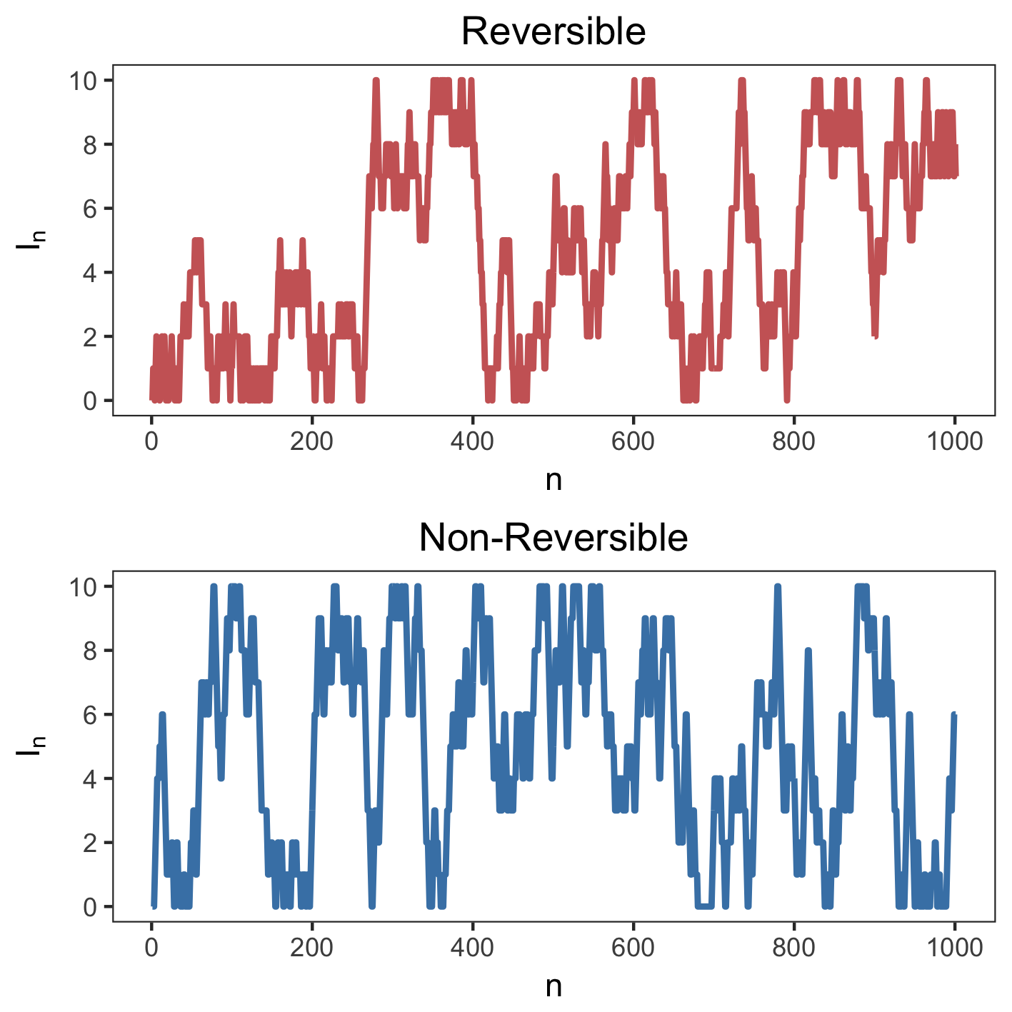
Refer to caption
Refer to caption
Figure 15: Sample trajectories of the component In0subscriptsuperscript𝐼0𝑛I^{0}_{n} of the index process for a Gaussian model with Λ=5Λ5\Lambda=5 with schedule 𝒫Nsubscript𝒫𝑁\mathcal{P}_{N} satisfying (169) for N=10𝑁10N=10 (left) and N=100𝑁100N=100 (right). The trajectories are run over 100N100𝑁100N iterations for reversible (top) and non-reversible (bottom) PT.
Refer to caption
Refer to caption
Figure 16: (Left) The local communication barrier for d=8,σ=1/2,1/10,1/100formulae-sequence𝑑8𝜎121101100d=8,\sigma=1/2,1/10,1/100 and σ0=1subscript𝜎01\sigma_{0}=1. (Right) The global communication barrier as a function of d𝑑d for τ=2,10,100𝜏210100\tau=2,10,100 and σ0=1subscript𝜎01\sigma_{0}=1. The solid line is the approximation λ^(β)^𝜆𝛽\hat{\lambda}(\beta) (respectively Λ^^Λ\hat{\Lambda}), resulting from Algorithm 4 (N=60𝑁60N=60 and n=10 000𝑛10000n=10\,000 scans) and the dotted line is the analytic expression from (168).

I.4.2 Ising model

We now compute numerically λ𝜆\lambda for the Ising model on a 2-dimensional lattice of size M×M𝑀𝑀M\times M with magnetic moment μ𝜇\mu. Note that the terminology “Ising” is technically incorrect since we are using a finite M𝑀M instead of an infinite lattice. The terminology “autologistic” would be more appropriate but we abuse the terminology “Ising” since it is widespread in the computational statistics literature. Similarly, when we talk about “phase transition” this should be interpreted as an approximate phase transition since M𝑀M is finite.

Using the notation xixjsimilar-tosubscript𝑥𝑖subscript𝑥𝑗x_{i}\sim x_{j} to indicate sites are nearest neighbours on the lattice, the target distribution is annealed by the inverse temperature β𝛽\beta and the tempered distributions are given by

π(β)(x)=1Z(β)exp(βxixjxixj+μixi).superscript𝜋𝛽𝑥1𝑍𝛽𝛽subscriptsimilar-tosubscript𝑥𝑖subscript𝑥𝑗subscript𝑥𝑖subscript𝑥𝑗𝜇subscript𝑖subscript𝑥𝑖\displaystyle\pi^{(\beta)}(x)=\frac{1}{Z(\beta)}\exp\left(\beta\sum_{x_{i}\sim x_{j}}x_{i}x_{j}+\mu\sum_{i}x_{i}\right). (170)

This is an M2superscript𝑀2M^{2} dimensional model which undergoes a phase transition as M𝑀M\to\infty at some critical inverse-temperature βcsubscript𝛽𝑐\beta_{c}. When μ=0𝜇0\mu=0 it is known that βc=log(1+2)/2subscript𝛽𝑐122\beta_{c}=\log(1+\sqrt{2})/2 [Baxter, 2007]. We consider experiments with μ=0𝜇0\mu=0 and with μ=0.1𝜇0.1\mu=0.1, the latter denoted “Ising with magnetic field” and abbreviated “magnetic” in composite figures.

We observe that λ𝜆\lambda exhibits very different characteristics in this scenario compared to the Gaussian model: it is not monotonic and is maximized at the critical temperature. Consequently, the optimal annealing schedule is denser near the phase transition. We also note from Figure 17 that both λ𝜆\lambda and ΛΛ\Lambda increases roughly linearly with respect to M𝑀M, similarly to the conclusion of Proposition 4, however here the conditions of Proposition 4 do not apply. As N𝑁N increases, the round trip rate of reversible PT decays to 0 and non-reversible PT increase towards (2+2Λ)1superscript22Λ1(2+2\Lambda)^{-1} as seen in Figure 18. This is consistent with Theorem 3.
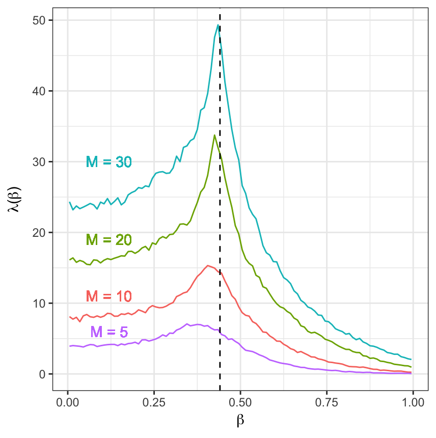
Refer to caption
Refer to caption
Figure 17: Estimate of the local communication barrier (left) and global communication barrier (right) for the Ising model with μ=0𝜇0\mu=0 and M=5,10,20,30𝑀5102030M=5,10,20,30. The vertical line is at the phase transition.
Refer to caption
Refer to caption
Figure 18: (Left) Optimal annealing schedule for the Ising model with M=20𝑀20M=20, Λ=13.33Λ13.33\Lambda=13.33 with N=30𝑁30N=30. The vertical line is at the phase transition. (Right) The round trip rates when M=20𝑀20M=20 with a uniform schedule (dashed) to the optimal schedule (solid) for both non-reversible (blue) and reversible (red) PT. The dotted horizontal line represents the approximation of the optimal round trip rate (2+2Λ^)1superscript22^Λ1(2+2\hat{\Lambda})^{-1}.
Refer to caption
Refer to caption
Figure 19: Further results on robustness to ELE violation on the Ising model with a magnetic moment, μ=0.1𝜇0.1\mu=0.1. Impact of increasing the number N𝑁N of parallel chains for an example where ELE is severely violated (only half the variables are updated at each exploration step). (Left) Estimated upper bound τ¯¯𝜏\bar{\tau}. This quantity is well estimated for any N𝑁N. (Right) Round trip rate τ𝜏\tau measured from the empirical index process trajectories. Dotted line shows τ¯¯𝜏\bar{\tau}. The result shows τ𝜏\tau approaches τ¯¯𝜏\bar{\tau} by increasing N𝑁N. This experiment suggests that the result in Theorem 3(c) may hold under more general conditions. Moreover since τ¯¯𝜏\bar{\tau} is well estimated even when the number of chains is modest, the gap between τ¯¯𝜏\bar{\tau} and observed τ𝜏\tau can be readily estimated.

I.4.3 Discrete-multimodal problem

Consider a discrete state space 𝒳={0,,2k}𝒳02𝑘\mathcal{X}=\{0,\dots,2k\}, and let 1Even:Ω{0,1}:subscript1EvenΩ011_{\mathrm{Even}}:\Omega\to\{0,1\} denote the indicator function for even numbers. Define π(x)a1Even(x)proportional-to𝜋𝑥superscript𝑎subscript1Even𝑥\pi(x)\propto a^{1_{\mathrm{Even}}(x)} for a>1𝑎1a>1 and π0(x)1proportional-tosubscript𝜋0𝑥1\pi_{0}(x)\propto 1 with V(x)=1Even(x)loga𝑉𝑥subscript1Even𝑥𝑎V(x)=-1_{\mathrm{Even}}(x)\log a. The distribution π𝜋\pi has k+1𝑘1k+1 modes located where x𝑥x is even with low probability “barriers” located at x𝑥x odd. The parameter a𝑎a controls the relative mass put on the modes. Therefore we have

π(β)(x)=aβ1Even(x)Z(β),superscript𝜋𝛽𝑥superscript𝑎𝛽subscript1Even𝑥𝑍𝛽\pi^{(\beta)}(x)=\frac{a^{\beta 1_{\mathrm{Even}}(x)}}{Z(\beta)}, (171)

where Z(β)=k+(k+1)aβ𝑍𝛽𝑘𝑘1superscript𝑎𝛽Z(\beta)=k+(k+1)a^{\beta}. A simple computation using (22) shows that the local communication barrier is,

λ(β)=k(k+1)aβloga(k+(k+1)aβ)2kaβloga(1+aβ)2.𝜆𝛽𝑘𝑘1superscript𝑎𝛽𝑎superscript𝑘𝑘1superscript𝑎𝛽2𝑘absentsuperscript𝑎𝛽𝑎superscript1superscript𝑎𝛽2\lambda(\beta)=\frac{k(k+1)a^{\beta}\log a}{(k+(k+1)a^{\beta})^{2}}\xrightarrow[k\to\infty]{}\frac{a^{\beta}\log a}{(1+a^{\beta})^{2}}. (172)

By integrating we obtain the global communication barrier between π𝜋\pi and π0subscript𝜋0\pi_{0},

Λ=k(k+1)(a1)(2k+1)(k+(k+1)a)ka12(a+1).Λ𝑘𝑘1𝑎12𝑘1𝑘𝑘1𝑎𝑘absent𝑎12𝑎1\displaystyle\Lambda=\frac{k(k+1)(a-1)}{(2k+1)(k+(k+1)a)}\xrightarrow[k\to\infty]{}\frac{a-1}{2(a+1)}. (173)

I.4.4 Mixture model

We consider a Bayesian mixture model with two mixture components. The likelihood for each component is a normal distribution with a non-conjugate Uniform(0,100)0100(0,100) prior on the standard deviation and a normal prior on the means (standard deviation of 100100100). We placed a uniform prior on the mixture proportion. We used simulated data generated from the model. While the mixture membership indicator latent random variables can be marginalized in this model, we sample them to make the posterior inference problem more challenging. Sampling these mixture membership random variables is representative of more complex models from the Bayesian non-parametric literature where marginalization of the latent variable is intractable; for example, this is the case for the stick-breaking representation of general completely random measures [Zhu et al., 2020].

In addition to the three MCMC methods described in the main text, we also ran baselines based on SMC and AIS, which are popular methods to explore complex posterior distributions. These methods also depend on the construction of a sequence of annealed distributions from prior to posterior. For the SMC and AIS baselines, to select the sequence of distributions we used an adaptive scheme based on relative ESS as described in [Zhou et al., 2016]. Diagnostics of the adaptation are shown in Figure 26. These methods were parallelized at the particle level. We set the number of particles to achieve a similar running time compared to NRTP, namely 2 00020002\,000 particles for SMC and 2 50025002\,500 particles for AIS. We found that the quality of the posterior approximation was highly dependent on performing several rounds of rejuvenations on the final particle population. The wall-clock time with 5 and 20 rounds of rejuvenation (SMC-5, SMC-20) was comparable to NRPT (1.778min, 2.302min) however the posterior approximation is markedly poor compared to NRPT. With 100 rounds of rejuvenation, the posterior approximation matches closely that of NRPT, however this brings the computation cost to 5.064min. AIS did not perform well since the weights were highly unbalanced in the last iteration, effectively resulting in an approximation putting all mass to a single particle.

I.4.5 Copy number inference

A copy number alteration is a widespread type of mutation in cancers. Whereas in healthy cells each non-sexual chromosomes comes in two copies, in certain cancer cells, chunks of chromosomes of small and large size are frequently deleted or duplicated [Beroukhim et al., 2010]—one extreme type of such event is a whole-genome duplication, in which the copy number of every genomic position is doubled. We consider the task of inferring the copy number for each location in the genome based on single-cell, whole genome data. For simplicity, we consider here a model for performing inference over the copy number profile of one individual cell at a time.

The data consists in the number of reads yi,csubscript𝑦𝑖𝑐y_{i,c} measured at different loci. Here i𝑖i denotes a sub-region or bin of a chromosome c𝑐c. We use the same binning method as [Lai et al., 2020]. The goal is to infer for each bin i𝑖i and chromosome c𝑐c an integer copy number xi,csubscript𝑥𝑖𝑐x_{i,c}. As previously reported in [Zahn et al., 2017], and confirmed in Figure 27, to a first order approximation the location parameter of the variable yi,csubscript𝑦𝑖𝑐y_{i,c} is determined by (1) the known GC contents of each bin, denoted gi,csubscript𝑔𝑖𝑐g_{i,c} and (2) the unknown copy number xi,csubscript𝑥𝑖𝑐x_{i,c}. Here instead of performing GC-normalization as a pre-processing step, as done in [Zahn et al., 2017], we perform GC-normalization jointly with copy number inference. We describe in this section how doing so allows us to capture the uncertainty over plausible whole-genome duplication events, and induces multimodal posterior distributions.

The single cell protocol used for the dataset considered here [Zahn et al., 2017] minimizes the PCR amplification biases so that after correcting the GC-bias, the count in a bin is approximately proportional to the copy number of the bin: logyi,c=f(θ,loggi,c)+log(xi,c)+ϵi,c,subscript𝑦𝑖𝑐𝑓𝜃subscript𝑔𝑖𝑐subscript𝑥𝑖𝑐subscriptitalic-ϵ𝑖𝑐\log y_{i,c}=f(\theta,\log g_{i,c})+\log(x_{i,c})+\epsilon_{i,c}, for xi,c>0subscript𝑥𝑖𝑐0x_{i,c}>0. Based on Figure 27 in Appendix J.4, we approximate f𝑓f using a latent quadratic function, and hence θ𝜃\theta is a global parameter containing the 3 coefficients specifying a quadratic polynomial. We assume ϵi,csubscriptitalic-ϵ𝑖𝑐\epsilon_{i,c} are independent zero-mean normal random variables with standard deviation σ𝜎\sigma. To model the prior information that copy number events affect contiguous regions of the genome, for each chromosome c𝑐c, we model the collection of random variables x1,c,x2,c,subscript𝑥1𝑐subscript𝑥2𝑐x_{1,c},x_{2,c},\dots using a hidden Markov model (HMM). The maximum copy number in each chromosome is modelled using a geometric random variable mcsubscript𝑚𝑐m_{c} with a shared latent parameter p𝑝p.

We placed an exponential prior on σ𝜎\sigma with rate 1/101101/10. We posit normal priors on the coefficients θ𝜃\theta (mean zero, variance 100). We put a uniform prior on p𝑝p. The transition probabilities of the Markov chain are determined by the marginals of a Juke Cantor model with a global rate parameter τ𝜏\tau. We put a unit exponential prior on τ𝜏\tau. Full model specification is available at https://github.com/UBC-Stat-ML/nowellpack/blob/multimodality-example/src/main/java/chromobreak/SingleCell.bl.

I.5 Multimodality of the examples considered

Figures 4 (bottom left), 22 and 23 support the multimodality of two of the examples considered in Section 7.3, namely the Ising and Spike-and-Slab examples. Multimodality of other examples considered in Section 7.1, 7.2, 7.4 and 7.5 is demonstrated in Figures 4, 27, 25, 28 and 29. Moreover, Figures 4, 25, 28 and 29 demonstrate that using standard MCMC is insufficient to explore these multimodal distributions.

I.6 Selection of π0subscript𝜋0\pi_{0}

In our experiments all Bayesian models considered have proper priors, and hence we set π0subscript𝜋0\pi_{0} to the prior in all these situations. The local exploration kernel in this case consists in an independent draw from the prior (performed by sorting the latent random variables according to a linearization of the partial order induced by the directed graphical model, and sampling their values according to these sorted laws).

For the Ising model, we let π0subscript𝜋0\pi_{0} denote a product of independent and identically distributed Bernoulli(1/2121/2) random variables, one for each node in the Ising grid. It is then straightforward to interpolate between this product distribution and the Ising model of interest using a geometric average. Independent sampling from π0subscript𝜋0\pi_{0} is used for the local exploration kernel at β=0𝛽0\beta=0.

Similarly, for the rotor (XY) model, we take π0subscript𝜋0\pi_{0} to be a product of independent and identically distributed Uniform(π,π𝜋𝜋-\pi,\pi) random variables, and we use a geometric interpolation between π0subscript𝜋0\pi_{0} and the target distribution.

Appendix J Supplementary figures for Section 7

J.1 Section 7.1
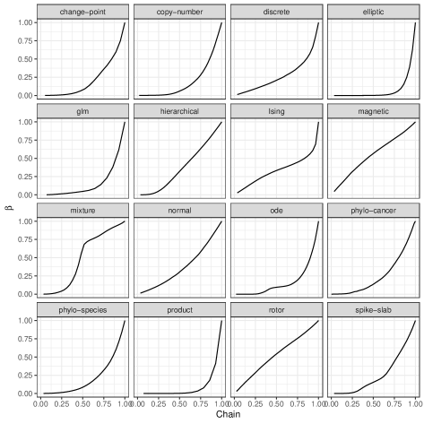
Refer to caption
Refer to caption
Figure 20: Top: Estimates of the schedule generator G𝐺G for 16 models. The abscissa denotes the normalized chain indices i/N𝑖𝑁i/N, the ordinates, parameters β𝛽\beta. The function G𝐺G is such that the partition G(0),G(1/N),G(2/N),,G(1)𝐺0𝐺1𝑁𝐺2𝑁𝐺1G(0),G(1/N),G(2/N),\dots,G(1) approximates equi-acceptance. Bottom: Estimates of ΛΛ\Lambda for 16 models. The abscissa denotes the schedule optimization round.

J.2 Section 7.3

Model (and dataset when applicable) Method N𝑁N s^^𝑠\hat{s} (%) Λ^^Λ\hat{\Lambda}
Spike-and-slab classification NRPT+SCM 151515 67.667.667.6 4.544.544.54
(RMS Titanic passengers data, [Hind, 2019]) ARR 666 36.336.336.3 3.823.823.82
MMV 666 39.939.939.9 3.613.613.61
NRPT 151515 67.267.267.2 4.594.594.59
Bayesian hierarchical model NRPT+SCM 343434 63.763.763.7 11.9611.9611.96
(historical rocket failure data, [McDowell, 2019]) ARR 2superscript22^{*} 0superscript00^{*} 1superscript11^{*}
MMV 151515 33.633.633.6 9.969.969.96
NRPT 343434 63.463.463.4 12.0812.0812.08
Wright-Fisher diffusion NRPT+SCM 151515 75.275.275.2 3.473.473.47
ARR 555 43.843.843.8 2.812.812.81
MMV 555 43.743.743.7 2.822.822.82
NRPT 151515 75.575.575.5 3.423.423.42
Ising model NRPT+SCM 151515 78.278.278.2 3.053.053.05
ARR 444 37.937.937.9 2.482.482.48
MMV 444 36.936.936.9 2.522.522.52
NRPT 151515 78.578.578.5 3.013.013.01
Figure 21: Summary statistics for the experiments in Section 7.3. The row marked with a star indicates failed optimization of one of the stochastic optimization schemes on the Bayesian hierarchical model.
Refer to caption
Refer to caption
Refer to caption
Figure 22: Examples of multimodality encountered in the Spike-and-Slab model applied to the RMS Titanic passenger dataset. Joint posterior distribution of the following regression parameters (1) passengerAge and passengerClass; (2) passengerAge and SiblingsSpousesAboard; (3) passengerClass and passengerClass2, the latter corresponding to an artificially duplicated regressor used to investigate the effect of co-linearity on the posterior approximation.
Refer to caption
Figure 23: Example of multimodality in an Ising model. Each facet is a posterior probability mass function, facet rows index the first 20 vertices of the Ising graph, facet columns, four posterior approximation methods. By symmetry, each marginal should place equal mass at spins 11-1 and 111. The multimodality is only correctly captured by our proposed algorithm (NRPT, third column, wall clock time of 7.250s, N=10𝑁10N=10). For the other methods, the posterior approximation either misses the other mode completely, namely when using AIS (left column, wall clock time of 5.723s, 1000 particles, relative ESS adaptive annealing schedule) or single-chain MCMC (second column, wall clock time of 1.439s), or, for annealed SMC (fourth column, wall clock time of 8.269s, 1000 particles, relative ESS adaptive annealing schedule), detects the multimodality but not their respective proportions. All wall clock time are reported for a 2.8 GHz Intel Core i7.

J.3 Section 7.4

Refer to caption
Refer to caption
Refer to caption
Figure 24: Diagnostics for the adaptive annealed SMC method (SCM), used as a benchmark on the Bayesian mixture problem. From left to right: (1) ESS as a function of the SMC iteration. Resampling is performed when the ESS drops below 1/2121/2; (2) annealing parameter as a function of the SMC iteration; (3) log normalization estimates at each resampling step.
Refer to caption
Refer to caption
Refer to caption
Refer to caption
Figure 25: Mixture modelling example: post burn-in trace plots of two model parameters (facet rows) for four MCMC methods considered (facet columns). The two parameters correspond to the location parameters of two exchangeable clusters. Correct MCMC exploration of this unidentifiable model requires label switching, providing a test bed for MCMC over multimodal targets. All methods use a computational budget lower or equal to NRPT’s.
Refer to caption
Refer to caption
Refer to caption
Refer to caption
Figure 26: Diagnostics for NRPT on the mixture modelling example. From left to right: (1) Estimate of the global communication barrier Λ^^Λ\hat{\Lambda} as a function of the schedule optimization round. (2) Average swap acceptance probability across the 30 chains as a function of the schedule optimization round. The final value is 72%percent7272\%. (3) Estimated communication barrier λ𝜆\lambda output by NRPT. The two peaks can be interpreted as transition points where the cluster membership indicator variables go from disorganized (all cluster membership variables are i.i.d. at β=0𝛽0\beta=0), to all taking the same value within a cluster. The two clusters having different number of data points and parameters induce two distinct transition points. The empirical behaviour observed is analogous to the phase transition found in statistical mechanics models such as the Ising model. Investigation of possible phase transitions in clustering models would be an interesting future direction of investigation, although somewhat orthogonal to this work. (4) Learning curves for the annealing parameters (ordinate axis, log scale) for the 303030 NRPT chains (colours) as a function of the schedule optimization round (abscissa).

J.4 Section 7.5
Refer to caption
Refer to caption
Refer to caption
Refer to caption
Refer to caption
Figure 27: Copy number inference: inputs and outputs. From left to right: (1) raw data, where each dot represent a genomic bin i,c𝑖𝑐i,c, with its abscissa showing loggi,csubscript𝑔𝑖𝑐\log g_{i,c} and its ordinate, logyi,csubscript𝑦𝑖𝑐\log y_{i,c}. (2) posterior distribution obtained from NRPT for the random function f(θ,)𝑓𝜃f(\theta,\cdot) obtained from NRPT. One translucent line f(θn,)𝑓subscript𝜃𝑛f(\theta_{n},\cdot) is drawn for each sampled θnsubscript𝜃𝑛\theta_{n}. Notice the bi-modality of the posterior distribution. (3) The approximation of the same posterior distribution based on a single chain misses one of the modes. (4) Two regions in chromosome 2 supporting a plausible genome duplication (and hence multimodality). We show here a sample index n𝑛n corresponding to the tetraploid mode in the second sub-panel. The dots show the data after GC-correction based on sample n𝑛n, i.e. exp(logyi,cf(θn,loggi,c))subscript𝑦𝑖𝑐𝑓subscript𝜃𝑛subscript𝑔𝑖𝑐\exp(\log y_{i,c}-f(\theta_{n},\log g_{i,c})). The line shows the imputed copy numbers at iteration n𝑛n. Notice the two small regions with odd copy numbers, around position 25 and just before position 200. (5) Same visualization as panel (4) but for a sample index n𝑛n corresponding to the diploid mode. Regions 25 and 200 cannot be explained without assuming genome duplication, however since the regions supporting duplication are small, the model remains uncertain about ploidy and hence multimodal.
Refer to caption
Refer to caption
Refer to caption
Refer to caption
Figure 28: Multimodality of the random variables mcsubscript𝑚𝑐m_{c} controlling the size of the copy number space for each chromosome c𝑐c. Each facet displays an approximate posterior probability mass function. Facet rows are indexed by chromosomes. Facet columns are indexed by posterior inference methods, which are all MCMC schemes ran for 5000 iterations. (1, 2) The multimodality arising from a weakly supported genome duplication is captured by NRPT, based on N=50𝑁50N=50 and N=25𝑁25N=25 respectively. (3) Results for an MCMC run based on the same exploration kernel misses the multimodality. (4) The stochastic adaptation method MMV fails to learn a schedule capable of performing round trips within the 5000 iterations and therefore misses the multimodality as well. See Section 7.5 for details.
Refer to caption
Figure 29: Enlarged version of Figure 12.
Refer to caption
Refer to caption
Refer to caption
Refer to caption
Figure 30: NRPT diagnostics on the copy number inference example. From left to right: (1) Estimate of the global communication barrier Λ^^Λ\hat{\Lambda} as a function of the scehdule optimization round. (2) Average swap acceptance probability across the 50 chains as a function of the schedule optimization round. (3) Estimated communication barrier λ𝜆\lambda output by NRPT. (4) Learning curve for the annealing parameters (ordinate axis, log scale) for the 505050 NRPT chains (colours) as a function of the schedule optimization round (abscissa).