ATM: An Open-Source Tool for Asteroid Thermal Modeling

Abstract

We publicly release ATM, a Python package designed to model asteroid flux measurements to estimate an asteroid’s size, surface temperature distribution, and emissivity. A number of the most popular static asteroid thermal models are implemented with the reflected solar light contribution and Kirchhoff’s law accounted for. Priors for fitted parameters can be easily specified and the solution, including the full multi-dimensional posterior probability density function, is found using Markov Chain Monte Carlo (MCMC). We describe the package’s architecture and discuss model and fitting validation. Data files with $\sim$ 2.5 million WISE flux measurements for $\sim$ 150,000 unique asteroids and additional Minor Planet Center data are also included with the package, as well as Python Jupyter Notebooks with examples of how to select subsamples of objects, filter and process data, and use ATM to fit for the desired model parameters. The entirety of the analysis presented here, including all the figures, tables, and catalogs, can be easily reproduced with these publicly released Notebooks. We show that ATM can match the best-fit size estimates for well-observed asteroids published in 2016 by the NEOWISE team (Mainzer et al., 2016) with a sub-percent bias and a scatter of only 6%. Our analysis of various sources of random and systematic size uncertainties shows that for the majority of over 100,000 objects with WISE-based size estimates random uncertainties (precision) are about 10%; systematic uncertainties within the adopted model framework, such as NEATM, are likely in the range of 10-20%. Hence, the accuracy of WISE-based asteroid size estimates is approximately in the range of 15-20% for most objects, except for unknown errors due to a possibly over-simplified modeling framework (e.g., spherical asteroid approximation). We also study optical data collected by the Sloan Digital Sky Survey (SDSS) and show that correlations of optical colors and WISE-based best-fit model parameters indicate robustness of the latter. Our analysis gives support to the claim by Harris & Drube (2014) that candidate metallic asteroids can be selected using the best-fit temperature parameter and infrared albedo. We investigate a correlation between SDSS colors and optical albedo derived using WISE-based size estimates and show that this correlation can be used to estimate asteroid sizes with optical data alone, with a precision of about 21% relative to WISE-based size estimates. After accounting for systematic errors, the difference in accuracy between infrared and optical color-based size estimates becomes less than a factor of two.

1 Introduction

Asteroid thermal flux modeling aims to estimate an asteroid’s size (volume-equivalent diameter, hereafter diameter) and surface temperature distribution, and sometimes other physical properties such as emissivity, from measured infrared (IR) fluxes. The largest dataset of infrared flux measurements for asteroids was recently contributed by the WISE survey (Wright et al., 2010) and analyzed by the associated NEOWISE team (Mainzer et al., 2011, and references therein). Flux measurements in four WISE bands provide strong constraints on asteroid sizes and emissivities as a function of wavelength. A series of papers that produced size estimates for about 164,000 asteroids, as well as constraints on asteroid emissivity properties, was reviewed and summarized by Mainzer et al. (2015).

It appears that the pioneering analysis by the NEOWISE team can be improved in various ways, as argued by Myhrvold (2018a, b). In particular, ignoring reflected sunlight can induce biases in estimated asteroid sizes and lead to underestimated size uncertainties. In addition, best-fit sizes can be biased due to assumptions on the priors for an asteroid’s emissivity as a function of wavelength, which varies with the chemical composition of an asteroid’s surface. Further biases are introduced by the use of fairly simplistic static thermal models to calculate volume-equivalent diameters. The need for improvements in data analysis was recently acknowledged by Wright et al. (2018), but it appears that a number of data analysis issues remain open. In particular, the behavior of systematic and random (statistical) uncertainties for the best-fit parameters remains an active research topic (see for example Wright, 2007; Mommert et al., 2018; Masiero et al., 2018a)

Given that the WISE dataset is by far the largest of its kind and will not soon be surpassed, it is prudent to focus on improved data analysis. We aim to contribute to such improvements by publicly releasing a new Python modeling tool, ATM (Asteroid Thermal Modeling), designed to enable easy fitting of the most common thermal models to WISE and other asteroid flux measurements. Data analysis software is often a crucial component in delivering scientific results, as vividly exemplified by this case, and thus discussions of scientific reproducibility and transparency can be greatly enhanced by collaborative software development and code sharing. Thanks to rapidly developing tools and technologies, such as Jupyter Notebooks, Python, and GitHub, performing these steps in open-source environment is now easier than ever. By releasing ATM we aim to increase reproducibility – a fundamental tenet of the scientific process.

In §2 we describe the mathematical/physical model underlying ATM, its Python implementation, and discuss model validation using observational and model data for asteroid sizes from the literature. The capabilities of ATM, with emphasis on various treatments of Bayesian priors when also fitting emissivity are further illustrated in §3 using three well-observed asteroids. In §4 we apply ATM to a “gold” sample of $\sim$7,000 best-observed asteroids from the NEOWISE dataset; in addition to best-fit diameters, we also obtain best-fit values for the emissivity of each asteroid across WISE bands W1 and W2. The best-fit sizes are compared to the values obtained by the NEOWISE team (the 2016 Planetary Data System version). In §5 we match the “gold” sample to optical data from the SDSS Moving Object Catalog, compute the visual albedo $p_{V}$, and study its correlation with optical colors. We also discuss how optical colors can be used to estimate $p_{V}$ and asteroid sizes when adequate infrared data are not available. Our results are summarized in §6.

As part of the ATM package release, we also include all data files used in this work including NEOWISE, Minor Planet Center, and SDSS Moving Object Catalog data. We provide Jupyter Notebooks with examples of how to select subsamples of objects, process and filter their flux measurements, and how to use ATM to estimate their diameters and infrared emissivities. All of the analysis presented here, including all the figures and tables, can be easily reproduced using the Notebooks released with the ATM package on GitHub. In particular, https://github.com/moeyensj/atm/blob/master/notebooks/README.md lists the Notebooks required to reproduce each figure in this paper.

2 ATM: An Open-Source Tool for Asteroid Thermal Modeling

A detailed discussion of the relevant physics implemented in asteroid thermal flux modeling, and a summary of models proposed in the literature, are presented in Myhrvold (2018a) and references therein. Here we only summarize the main results needed to understand how ATM works and what it computes. We also describe its Python implementation and discuss model validation using observational and model data for asteroid sizes from literature.

2.1 The Asteroid Flux Model Summary

We first introduce $F_{\nu}(\lambda)$: the specific flux (flux per unit frequency, $\nu$) from an object. The SI units for $F_{\nu}$ are W m^-2 Hz^-1 (= 10³ erg cm^-2 s^-1). The specific flux can also be defined per unit wavelength, $F_{\lambda}$, using energy conservation $F_{\nu}|d\nu|=F_{\lambda}|d\lambda|$ and $\lambda\nu=c$. The choice of $F_{\nu}$, as opposed to $F_{\lambda}$, is completely arbitrary. Similarly, the running variable can be either $\lambda$ or $\nu$, and the choice of $\lambda$ is more convenient in this context.

The model flux from an asteroid, $F_{\nu}^{ast}(\lambda)$, corresponding to flux detected by the observer, $F_{\nu}^{obs}(\lambda)$, is the sum of the emitted thermal flux controlled by the asteroid’s surface temperature distribution, and the portion of the incident solar flux reflected by the asteroid,

$$F_{\nu}^{ast}(\lambda)=F_{\nu}^{th}(\lambda)+F_{\nu}^{ref}(\lambda).$$ (1)

A given model spectrum $F_{\nu}^{ast}(\lambda)$, corresponding to observational quantity $F_{\nu}^{obs}(\lambda)$, is integrated over the bandpass (assumed known hereafter) to obtain observed in-band model flux for a given instrument. For example, Wright (2013) has derived simple quadrature formulae that can be used to efficiently and accurately compute in-band fluxes for the four WISE bands from model flux $F_{\nu}^{ast}(\lambda)$.

Both $F_{\nu}^{th}(\lambda)$ and $F_{\nu}^{ref}(\lambda)$ depend on the relative positions of the Sun, the asteroid and the observer, the asteroid’s diameter $D$, and the asteroid’s emissivity, $\epsilon(\lambda)$, which controls the balance between absorbed/emitted and reflected incident flux. These relative positions are fully described by the asteroid-Sun distance, $r$, asteroid-observer distance, $\Delta$, and the angle subtended on the asteroid’s surface by the lines of sight towards the Sun and the observer, the so-called phase angle, $\alpha$. Hereafter we assume that asteroid orbital parameters are known and that $r$, $\Delta$ and $\alpha$ can be easily computed using standard and readily-available tools (e.g., the JPL HORIZONS service; OpenOrb, Granvik et al., 2015). To simplify nomenclature, we do not explicitly list these independent variables, unless necessary to avoid confusion.

2.1.1 The emitted flux

The observed thermal flux is obtained by integrating the emitted thermal flux per unit area over the visible surface of the asteroid,

$$F_{\nu}^{th}(\lambda)=\left({D\over 2\,\Delta}\right)^{2}\,\epsilon(\lambda)\int_{-\pi/2}^{\pi/2}\int_{-\pi/2+\alpha}^{\pi/2+\alpha}\pi B_{\nu}\left(T(\theta,\phi),\lambda\right)\cos(\theta-\alpha)\cos^{2}(\phi)d\theta d\phi,$$ (2)

where $\theta$ and $\phi$ are the integration variables over the asteroid’s surface (here we use geographic coordinates with $\theta=0$ and $\phi=0$ at the subsolar point, and both ranging from $-\pi$ to $\pi$; note that Myhrvold 2018a used ISO coordinates with $0<\phi<2\pi$), and $B_{\nu}$ is the Planck function.

It is implied that, in this context of thermal emission, asteroids are approximated as perfect spherical Lambertian emitters which follow Lambert’s cosine rule (unlike scattered light, which shows a strong opposition surge – a peaked reflectance for phase angles near zero).

The temperature variation across an asteroid’s surface is model dependent. ATM implements the three most common thermal models: the Standard Thermal Model (STM), the Fast Rotating Model (FRM), and the Near-Earth Asteroid Thermal Model (NEATM). For a comparison of these models and an analysis of their validity, please see Wright (2007), Mommert et al. (2018), and references therein. Common to all models is a temperature scale set by the so-called sub-solar temperature, $T_{ss}$, which is the highest temperature on the asteroid’s surface. Depending on the adopted model, the temperature variation across the surface can range in complexity from being constant to having a strong temperature gradient from the subsolar point (e.g., see Fig. 1 in Mommert et al. 2018).

The NEATM model uses a multiplicative correction factor (e.g., for surface roughness) to eq. 2 called the“beaming parameter”, $\eta$. For a more detailed discussion of this parameter, please see Myhrvold (2018a). The $\eta$ parameter is not constant and can vary with the observer’s location (Wright, 2007).

Given a model parameter for the temperature scale, $T_{1}$, defined as the sub-solar temperature when $r=1$ A.U., the sub-solar temperature is simply

$$T_{ss}=\left({1\,{\rm A.U.}\over r}\right)^{1/2}\,T_{1}.$$ (3)

Unlike $T_{ss}$, which depends on the asteroid-Sun distance, $T_{1}$ is nearly constant for a given asteroid (not exactly constant because of its slight dependence on $\eta$, see eq. 4 below).

The energy balance, discussed below, connects $T_{1}$ with the incident solar flux, an asteroid’s physical properties and other model parameters. Myhrvold (2018a) made an important point that when fitting a model to data, all the other parameters are not directly relevant – it is only $T_{1}$ that controls the model fluxes and thus it is only $T_{1}$ that is directly constrained by the infrared flux data for a given observer’s position.

2.1.2 The energy balance and the meaning of best-fit parameter $T_{1}$

Using the energy balance equation that equates the absorbed incident solar flux with the flux emitted by an asteroid, it can be shown (e.g., see Myhrvold 2018a and references therein) that

$$T_{1}=\left({S(1-A)\over\sigma\eta\epsilon_{B}}\right)^{1/4},$$ (4)

where $S$ is the solar constant at 1 A.U. ($S=1360.8$ Wm^-2), $\sigma=5.67\times 10^{-8}$ W m^-2 K^-4 is the Stefan-Boltzmann constant, and $A$ and $\epsilon_{B}$ are appropriately wavelength-averaged values of $1-\epsilon(\lambda)$ and $\epsilon(\lambda)$ over the incident and thermal flux distributions, respectively (for details, please see §3 in Myhrvold 2018a). It is usually assumed that $\epsilon_{B}=0.9$, but the exact value is not crucial to modeling once the beaming parameter $\eta$ is introduced – it is only the $\eta\epsilon_{B}$ product that can be constrained using best-fit $T_{1}$. Another conventional approximation is

$$A\approx A_{V}=p_{V}\,q,$$ (5)

where $A_{V}$ is the Bond albedo (limited to the range 0–1), $p_{V}$ is the geometric albedo in the visible band (can be larger than 1), and $q$ is the empirically-derived phase integral. In the H-G magnitude system introduced by Bowell et al. (1989), $q(G)=0.29+0.684G$, where $G$ is the slope parameter of the phase function. A common assumption, when G is unknown, is $G=0.15$. Therefore, the best-fit $T_{1}$ can be used to estimate $p_{V}$, given the value of the $\eta\epsilon_{B}$ product.

The geometric albedo can also be constrained, when the asteroid’s diameter, $D$, is known, using flux measurements at wavelengths sufficiently short for flux to be dominated by the reflected incident solar flux. For example, in the visual band

$$p_{V}=\left({1,329\,{\rm km}\over D}\right)^{2}\,10^{-0.4H},$$ (6)

where $H$ is the asteroid’s absolute magnitude in the visual band. When such measurements are available, the two constraints for $p_{V}$ can be used to estimate the beaming parameter, $\eta$, or to simply check the model’s internal consistency.

2.1.3 The reflected flux

The reflected flux is proportional to an asteroid’s reflectivity, $\rho(\lambda)$, with $\rho(\lambda)=1-\epsilon(\lambda)$ via Kirchhoff’s law,

$$F_{\nu}^{ref}(\lambda)=\left({D\over 2\,\Delta}\right)^{2}\,\frac{\Psi(\alpha,G)}{q(G)}\,\left[1-\epsilon(\lambda)\right]\,F_{\nu}^{\sun}(\lambda),$$ (7)

where the H-G phase function, $\Psi(\alpha,G)$, and empirically derived phase integral, $q(G)$, are purely geometric quantities that account for phase effects (Bowell et al., 1989).

The incident solar flux, $F_{\nu}^{\sun}(\lambda)$, at a distance $r$ from the Sun, is given by

$$F_{\nu}^{\sun}(\lambda)=\left({R_{\sun}\over r}\right)^{2}\,\pi\,B_{\nu}(T_{\sun},\lambda),$$ (8)

where $T_{\sun}=5,778$ K and $R_{\sun}=0.00465$ A.U. Therefore, when $\epsilon(\lambda)$ is known, the reflected flux is fully determined for a given observing geometry (note also that a fully known $\epsilon(\lambda)$ implies a given value of $p_{V}$).

2.1.4 Fitting Model Fluxes to Data

The likelihood of obtaining $N$ observed fluxes, $F^{obs}_{i}$, given model predictions, $F_{i}^{ast}$, can be written as (for details see, e.g., Chapter 4 in Ivezić et al. 2014)

$$L=\prod_{i=1}^{N}{1\over\sqrt{2\pi(\sigma_{i}^{2}+\Sigma^{2})}}\exp{\left({-(F^{obs}_{i}-F_{i}^{ast})^{2}\over 2\,(\sigma_{i}^{2}+\Sigma^{2})}\right)},$$ (9)

where $\sigma_{i}$ is the flux measurement uncertainty and $\Sigma$ accounts for variability. Assuming flat Bayesian priors for fitted model parameters, maximizing this likelihood function is equivalent to maximizing the Bayesian posterior probability density function. ATM also supports the Jeffreys’ priors (flat distributions in $\log(D)$ and $\log(T_{1})$, for details see Chapter 5 in Ivezić et al. 2014).

The above expression assumes that the scatter of flux measurements around predicted model values follows a Gaussian distribution with standard deviation (measurement uncertainty) $\sigma_{i}$. In practice, most asteroids show variability with amplitudes ($\sim 1$ mag) exceeding typical measurement uncertainties ($\leq$0.2 mag for SNR$\geq 5$). This variability is mostly due to non-spherical shapes, which are not captured by the model. For this reason, the likelihood expression includes the $\Sigma^{2}$ term. Given that $\Sigma\gg\sigma_{i}$ for reasonably high SNR, we have $\sigma_{i}^{2}+\Sigma^{2}\approx\Sigma^{2}$, which is presumed constant for a given asteroid. While it does not influence the values of the best-fit parameters, $\Sigma$ does control their uncertainty. Following Masiero et al. (2018c), we adopt $\Sigma=0.2$ mag as typical uncertainty due to variability.

When emissivity $\epsilon(\lambda)$ is assumed known, the best-fit model parameters are effectively obtained by maximizing the log-likelihood in magnitude space, as a function of two free parameters, $D$ and $T_{1}$ (for a discussion of emissivity fitting, see the next section),

$$ln(L)={\rm const.}-\sum_{i=1}^{N}\left[m^{obs}_{i}-m_{i}^{ast}(D,T_{1})\right]^{2},$$ (10)

where $m^{obs}_{i}$ are observed magnitudes and $m_{i}^{ast}$ are their model predictions ($m=-2.5\,\log_{10}(F)+{\rm const.}$).

2.1.5 The treatment of emissivity, $\epsilon(\lambda)$

The assumed priors for $\epsilon(\lambda)$ play an important role in determining an asteroid’s size. Technically, all fitted parameters require their prior probability distributions to be specified (for a discussion of Bayesian priors, see, for example, Chapter 5 in Ivezić et al. 2014). When $\epsilon(\lambda)$ is assumed known, these priors effectively become the Dirac $\delta$ functions.

When $\epsilon(\lambda)$ is assumed known, in principle even just two infrared flux measurements can constrain an asteroid’s diameter $D$ and temperature $T_{1}$. In essence, the measured color (i.e. the ratio of the two measured fluxes) constrains $T_{1}$ and the overall flux level constrains $D$. When measurement errors are present, the constraints become more complex, as discussed further below in the model validation section (§2.3). If more than two infrared flux measurements are available, $\Sigma$ is known from light curve analysis, and measurement errors are sufficiently small, the model fluxes can be checked for internal consistency using statistical tests such as $\chi^{2}$.

When $\epsilon(\lambda)$ is treated as a free parameter, care must be taken to avoid the $D\epsilon$ degeneracy when only thermal fluxes are measured: in eq. 2 parameters $D$ and $\epsilon$ appear only as a product $D^{2}\epsilon$. This degeneracy can be broken when flux measurements at wavelengths where the reflected light component is non-negligible are available. Because in eq. 7 the reflected flux is proportional to $D^{2}(1-\epsilon)$ rather than proportional to $D^{2}\,\epsilon$, the $D-\epsilon$ degeneracy is broken and both $\epsilon$ and $D$ can be estimated. The larger the contribution of the reflected flux to the total flux, the less correlated are the best-fit values of $\epsilon$ and $D$. We return to this point in §2.3.

In reality, a rather substantial variation in $\epsilon(\lambda)$ is observed for asteroids (e.g., see Fig. 1 in Myhrvold 2018a). If more than two flux measurements are available, as is the case for NEOWISE data with four bands, parameters from a judiciously chosen parameterization of $\epsilon(\lambda)$ can also be fit to data. In the case of four bandpasses, up to two such parameters can be well constrained (in addition to $D$ and $T_{1}$, for the total of four fitted parameters).

Unknown functions are often specified as power laws with two free parameters: the power-law index and its overall normalization. This common approximation would work poorly given the $\epsilon(\lambda)$ functions observed for asteroids. Instead, motivated by the observed behavior of the $\epsilon(\lambda)$ functions, we consider an ansatz (“a simplified procedure”, or “a provisional mathematical assumption”) where we fit $\epsilon_{W1W2}$, the value of $\epsilon(\lambda)$ in the WISE bands 1 and 2, and $\epsilon_{W3W4}$, the value of $\epsilon(\lambda)$ in the WISE bands 3 and 4. In other words, we approximate $\epsilon(\lambda)$ as a step function $\epsilon(\lambda)=\epsilon_{W1W2}$ for $\lambda<6\hbox{$\mu\mathrm{m}$}$, and $\epsilon(\lambda)=\epsilon_{W3W4}$ for $\lambda>6\hbox{$\mu\mathrm{m}$}$. Because the two shortest WISE bands include substantial contribution of reflected flux (e.g., see Figure 1 in Myhrvold 2018a), constraints can be placed on $\epsilon_{W1W2}$ and $\epsilon_{W3W4}$ for well-observed asteroids. We discuss these constraints in more detail in the next section. We note that asteroids with sizes estimated by other means (e.g., from occultation or radar measurements) represent an invaluable sample for constraining the behavior of $\epsilon(\lambda)$ among the asteroid population.

2.2 Model Implementation: ATM

We now briefly describe the ATM code architecture and highlight some aspects of its functionality. ATM is built on two bespoke Python classes: the ‘observatory’ and ‘model’ classes. The observatory class is used to describe an observatory’s filter throughput curves as a function of wavelength. In the case of WISE, these are the modified quadrature formulae provided by Wright (2013). The model class has placeholder functions for how a thermal model describes the surface temperature distribution on a model asteroid, how the observing geometry is taken into account, and how the model integrates emitted flux over the surface of a model asteroid of unit diameter. The instances of the two classes, called objects, can then be passed as arguments with physical parameters ($D$, $T_{ss}$, $\epsilon$, $p$, $G$) and observing parameters ($\alpha$, $r$, $\Delta$) to a series of functions. These functions calculate predicted in-band fluxes with and/or without reflected sunlight for the given observatory. Additionally, the model class can be passed separately to a different series of functions to generate model spectral energy distributions (SEDs) at a range of desired wavelengths.

As indicated by Myhrvold (2018a), fitting for different desired parameters and integrating the emitted flux on the fly can be slow. To make modeling and subsequent fitting more computationally tractable, ATM comes with emitted flux lookup tables generated for each thermal model at each WISE quadrature wavelength and at a range of wavelengths at 1 micron intervals between 1 and 30 microns. The lookup tables are functions of a grid of $T_{ss}$ and $\alpha$ values and contain $\sim$ 800,000 saved integration evaluations per table.

To conduct MCMC sampling, ATM uses the pymc3 (Salvatier et al., 2016) package. pymc3 is a robust Python probabilistic programming and Bayesian inference package and it allows for multi-threaded sampling of the posterior; the ATM lookup table implementation in combination with pymc3 allows 4,000 samples to be extracted in approximately 40 seconds on a moderate CPU. Each sampling chain requires a single thread, hence, sampling the posterior with 10 chains would require 10 threads and, because pymc3 support parallelization, it takes the same amount of time to sample as a single chain. Given a set of asteroid flux measurements for either a single object or multiple objects, with assumptions on priors for fitting parameters, the user can fit for any combination of parameters as defined by Eq 2. Should the user decide to constrain emissivity as described in §2.1.5, this task too is made simple by the use of several keyword arguments in the fitting function that describe how emissivity and albedo should be constrained and calculated.

We refer the reader to the GitHub repository for further information on the modeling code. The Notebooks used to validate the code are located here: https://github.com/moeyensj/atm/tree/master/notebooks/validation/. The Notebooks used to analyze the WISE sample of data (presented in the following sections) are located here: https://github.com/moeyensj/atm/tree/master/notebooks/analysis/. A Notebook showing how different assumptions regarding emissivity and albedo affect the modeling and retrieval of physical parameters is located here: https://github.com/moeyensj/atm/tree/master/notebooks/analysis/single_object_90367.ipynb.

2.3 ATM Validation

No complex software system can be fully trusted without extensive validation and verification steps. We validate and verify the ATM code in two steps. First, we generate synthetic fluxes from a hypothetical asteroid using given $D$, $T_{1}$, and $\epsilon(\lambda)$, and then use ATM to perform Markov Chain Monte Carlo (MCMC) fitting to recover the input parameters. This step serves as a validation of internal code consistency. Second, physical validation is performed using a few studies from the literature, where asteroid sizes are known independently from infrared flux measurements (e.g., from radar measurements and stellar occultation measurements).

2.3.1 Validation of the internal code consistency

Figure 1: The solid line shows the synthetic spectral energy distribution (SED) generated using the NEATM model for an asteroid with $D=1$ km, $T_{1}=422$ K, $\epsilon(\lambda)=0.7$, asteroid-Sun distance of 3 A.U., and an observer at 2 A.U. The four symbols with error bars correspond to the four in-band fluxes for the WISE observatory at the same distance from the asteroid. The error bars reflect the assumed variability amplitude but the implied scatter is not shown in this plot. The three other lines show the best fits obtained with ATM (see text). The two solid lines are indistinguishable. This figure was generated using notebooks/validation/example_synthetic_changingNumObservations.ipynb.

Figure 2: The posterior probability density function (pdf) for the case of fitting asteroid diameter $D$ (in m) and temperature parameter $T_{1}$ (in Kelvin; see eq. 4). The equivalent 1$-\sigma$ uncertainties for $D$ and $T_{1}$, measured as standard deviation of the marginal probability distributions (shown as histograms; the vertical lines are true input values), are 8.6% and 4.9%, respectively. Note the strong covariance between $D$ and $T_{1}$: a smaller $D$ is compensated by higher $T_{1}$. The best-fit SED is shown in Fig. 1. This figure was generated using notebooks/validation/example_synthetic_changingNumObservations.ipynb.

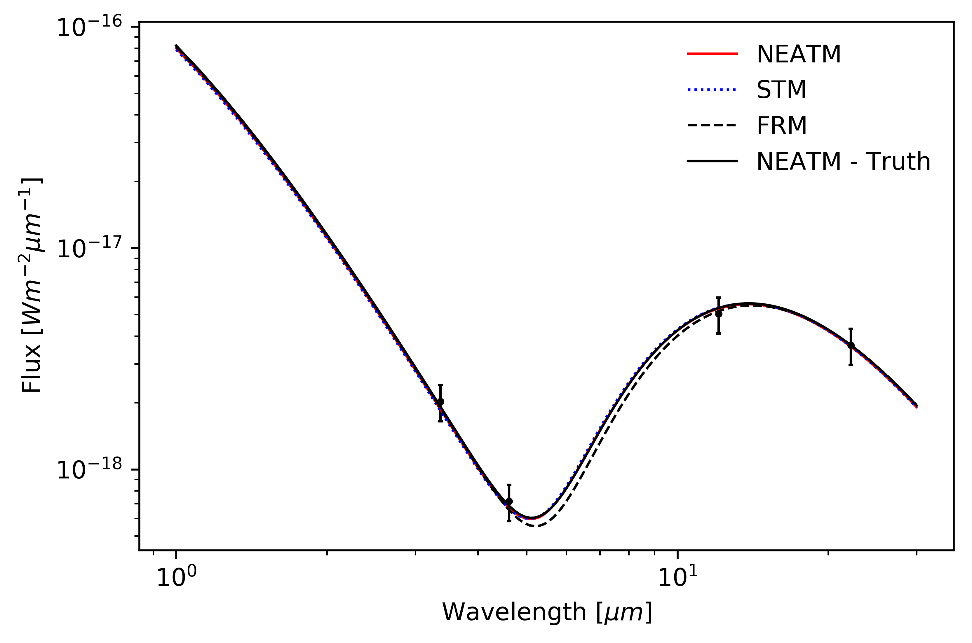
We generate synthetic fluxes in the four WISE bandpasses using an asteroid with $D=1$ km, $T_{1}=422$ K, $\epsilon(\lambda)=0.7$, and asteroid-Sun distance of 3 A.U. The observatory is placed at 2 A.U. from the asteroid. The synthetic fluxes generated using the NEATM model are shown in Fig. 1. The four symbols with error bars correspond to the four in-band fluxes for the WISE observatory. As evident, the flux in the bluest band is dominated by the reflected flux component, while the two reddest bands are dominated by the emitted flux component. When fitting for $D$ and $T_{1}$ using “observational” constraints in the four WISE bands, we add Gaussian scatter to each flux with a standard deviation of 20%. This scatter reflects the variability amplitude $\Sigma$ from eq. 9.

The synthetic model flux, generated using the NEATM model, is fit using MCMC and three different thermal models implemented in ATM: NEATM, STM and FRM. We use 20 chains, each with 3,000 samples and 500 burn-in samples. The best-fit parameters obtained using the STM and FRM models are very similar, but not identical, to the parameters obtained with the correct NEATM model. The three best-fit SEDs for the fiducial validation case are shown in Fig. 1.

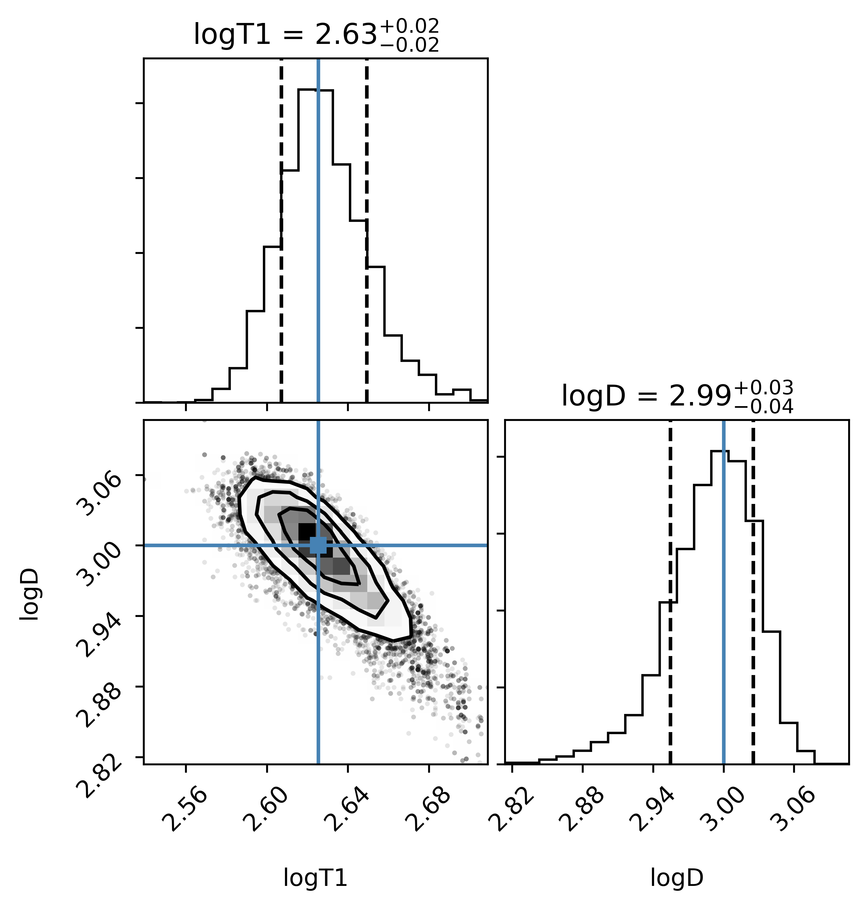
The posterior probability density function (pdf) for the NEATM fitting case is shown in Fig. 2. Note that the use of full multi-dimensional pdf for the analysis of constraints on the model parameters is superior to using the so-called “point estimates” obtained by maximum likelihood methods (e.g., the least squares method). A strong covariance between $D$ and $T_{1}$ is clearly visible: a smaller $D$ is compensated by higher $T_{1}$, with a bias (as well as scatter) in best-fit $D$ twice as large as the corresponding $T_{1}$ bias (because the observed flux approximately scales with $D^{2}T_{1}^{4}$). The equivalent 1$-\sigma$ uncertainties for $D$ and $T_{1}$ are 8.6% and 4.9%, respectively. These uncertainty levels can be approximately explained from first principles: given the flux uncertainty of 20% and 4 data points, the overall flux normalization uncertainty is about 10% (=20%/$\sqrt{4}$). If $T_{1}$ were known, the best-fit uncertainty for $D$ would be about 5%, and if $D$ were known, the best-fit uncertainty for $T_{1}$ would be about 2.5%. Given the covariance between best-fit $D$ and $T_{1}$, their expected uncertainties are about twice as large (see Fig. 2), in good agreement with the MCMC results.

When the number of epochs $N$ is increased, we find that the fitting uncertainty for the best-fit parameter decreases as $N^{-1/2}$, as expected. The fitting uncertainty increases approximately linearly with the assumed flux uncertainty ($\Sigma=0.2$ mag, presumably due to variability, rather than due to measurement uncertainties). For example, with $\Sigma=0.1$ mag and 25 observing epochs (each with four WISE fluxes), the fitting uncertainty for the best-fit parameters $D$ and $T_{1}$ decreases by about a factor of ten, to 0.92% and 0.52%, respectively. Of course, here we are using the same model for fitting as was used to generate the synthetic flux – in reality, such small uncertainties are essentially impossible due to numerous systematic shortcomings of idealized thermal models (and uncertain $\epsilon(\lambda)$ – see below).

These tests assumed that the correct values of $\epsilon(\lambda)$ are known a priori. When we set $\epsilon_{W1W2}$ to an incorrect value of 0.8, instead of the true input value of 0.7, we found that the best-fit value of $D$ was biased by as much as 22%. Therefore, even though formal fitting precision can be high, the accuracy of fitted parameters can be significantly worse.

We investigated next how the precision of the best-fit $D$ and $T_{1}$ decreases when emissivity $\epsilon(\lambda)$ is also fit. Following discussion in §2.1.5, we fit $\epsilon_{W1W2}$, the value of $\epsilon(\lambda)$ in the WISE bands 1 and 2, and assume that $\epsilon_{W3W4}$, the value of $\epsilon(\lambda)$ in the WISE bands 3 and 4, is known. In other words, we assume a flat prior in the range 0 to 1 for $\epsilon_{W1W2}$, and a Dirac $\delta$ function for $\epsilon_{W3W4}$, centered on its true value. The posterior pdf is shown in Fig. 3. The differences compared to the posterior pdf in Fig. 2 are substantial; for example, the equivalent 1$-\sigma$ uncertainties for $D$ and $T_{1}$ increased by about a factor of three: from 8.6% and 4.9% to 30% and 12%, respectively. In addition to the covariance between $D$ and $T_{1}$, both parameters show covariances with $\epsilon_{W1W2}$. A larger $\epsilon_{W1W2}$ can be compensated by a lower $T_{1}$ or a larger $D$. For example, a 0.1 uncertainty in $\epsilon_{W1W2}$ can induce a $\sim$25% uncertainty in $D$! Given that typically $\epsilon(\lambda)$ is not known to better than 0.05, it follows that uncertainty of best-fit $D$ is unlikely below $\sim$10% (in agreement with recent analysis by Wright et al. 2018 and Masiero et al. 2018a).

Figure 3: Analogous to Fig. 2, but here for the case of fitting three free parameters: asteroid diameter $D$, temperature parameter $T_{1}$, and the value of $\epsilon(\lambda)$ in the WISE bands 1 and 2, $\epsilon_{W1W2}$. Although all other simulation and fitting parameters are the same as is in Fig. 2, the differences between the posterior pdfs are substantial. For example, the equivalent 1$-\sigma$ uncertainties for $D$ and $T_{1}$ increased from 8.6% and 4.9% to 30% and 12%, respectively. In addition to the covariance between $D$ and $T_{1}$, both parameters show covariances with $\epsilon_{W1W2}$. Compared to $D$ and $T_{1}$, posterior constraints on $\epsilon_{W1W2}$ are much weaker. This figure was generated using notebooks/validation/example_synthetic_changingNumObservations.ipynb.

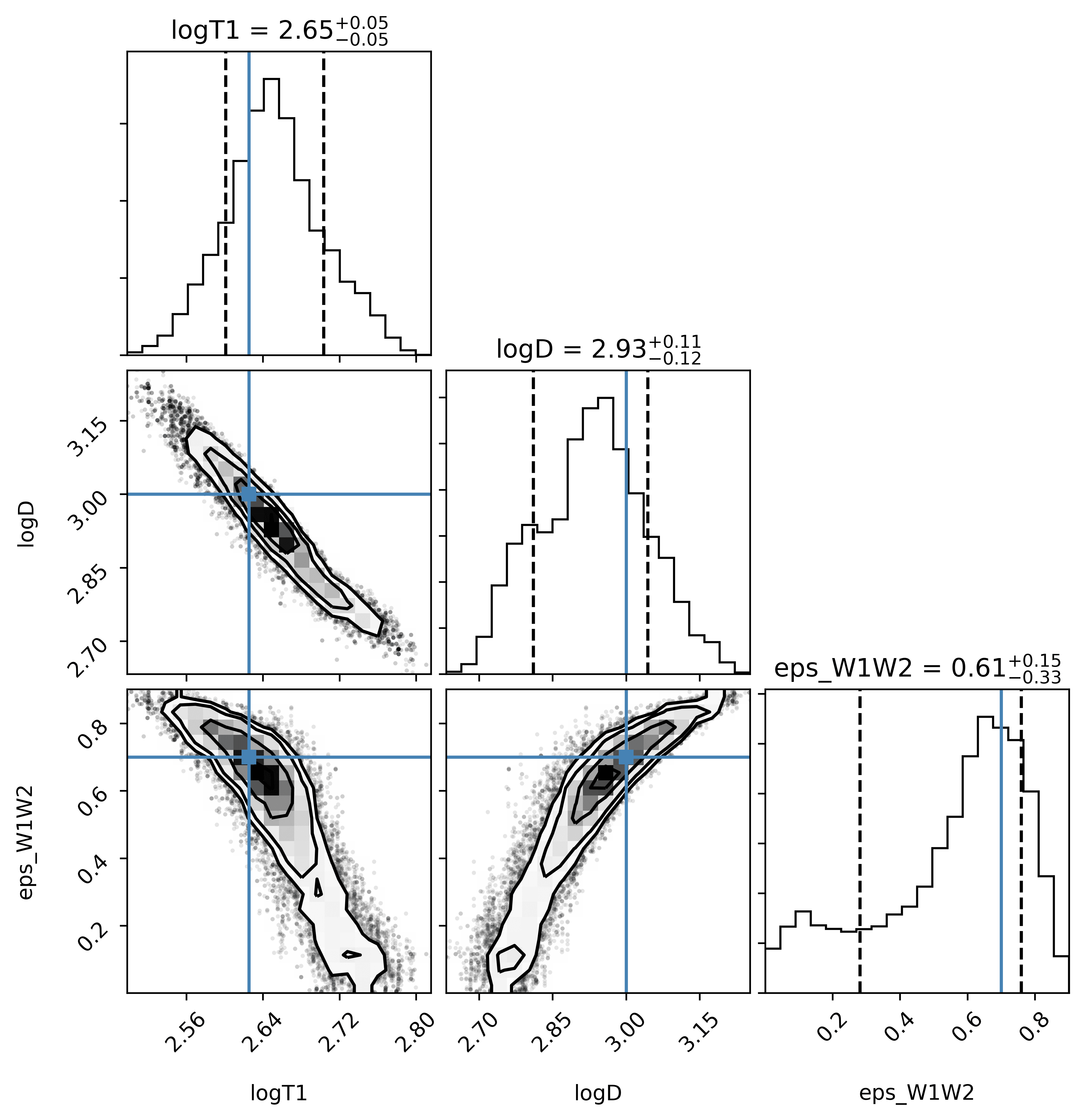
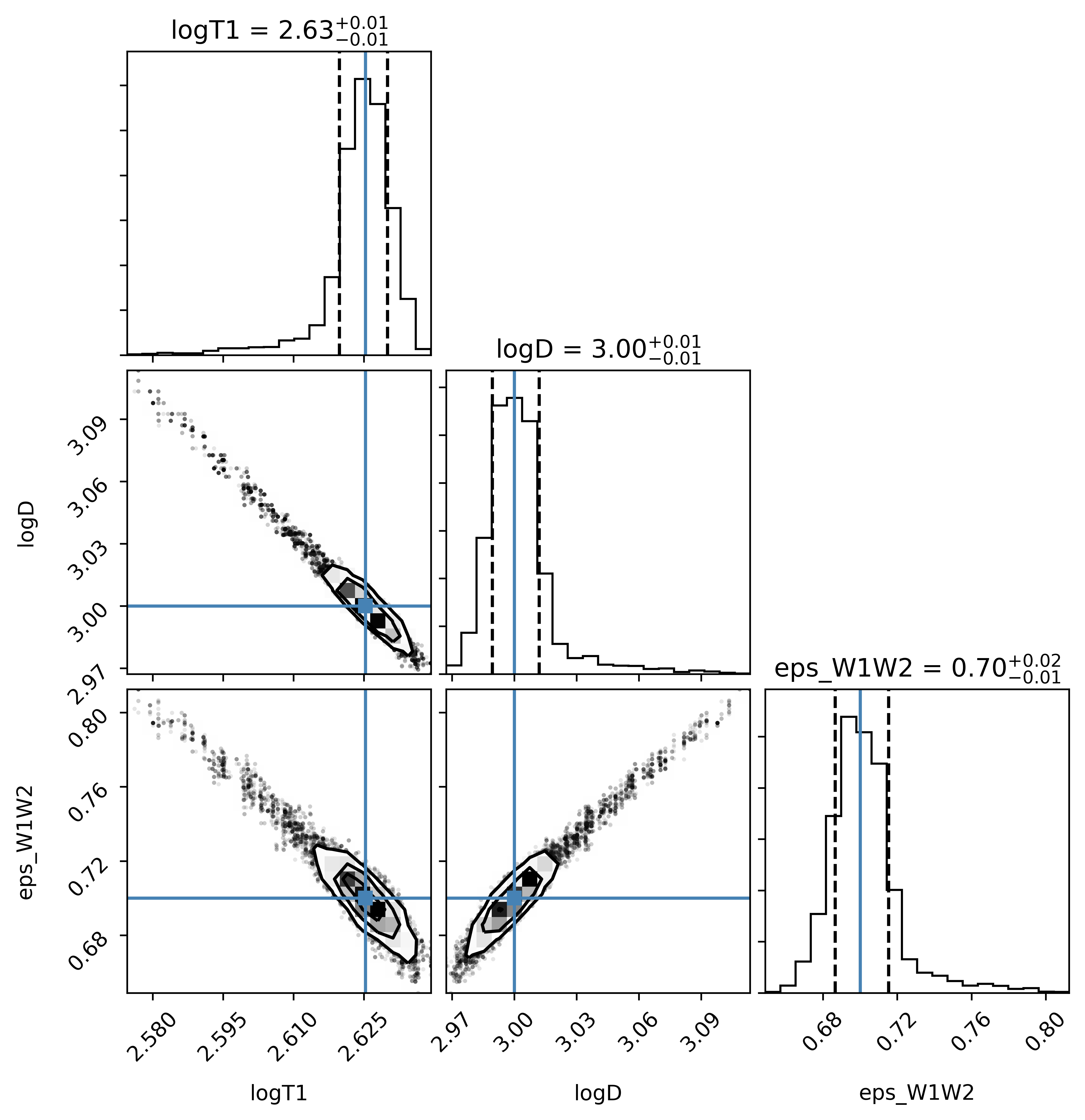
Compared to $D$ and $T_{1}$, the posterior constraint on $\epsilon_{W1W2}$ is much weaker. The standard deviation for the marginal distribution of $\epsilon_{W1W2}$ shown in Fig. 3 is 0.23, but note that this marginal pdf is far from Gaussian. The fitting constraints on all three free parameters, and $\epsilon_{W1W2}$ in particular, improve as the number of data points increases and the scatter $\Sigma$ decreases. Fig. 4 shows the posterior pdf when synthetic data include 25 epochs (each with four WISE fluxes) instead of one in Fig. 3, and with flux uncertainty of $\Sigma=0.1$ mag, instead of 0.2 mag. As evident, the posterior constraints for all three fitted parameters are significantly improved. The standard deviations for the marginal distributions are 2.5% for $D$, 1.1% for $T_{1}$ and 0.014 for $\epsilon_{W1W2}$ (recall that in the case of fitting only $D$ and $T_{1}$, their uncertainties were equal to 0.92% and 0.52%, respectively, using the same number of observations and the same value of $\Sigma$). Therefore, adding $\epsilon_{W1W2}$ as a free parameter results in about twice as large statistical uncertainties for the best-fit size $D$.

Figure 4: Analogous to Fig. 3, but here with better observational constraints: 25 epochs (each with four WISE fluxes) instead of one, and with flux uncertainty $\Sigma$ of 0.1 mag, instead of 0.2 mag. Note the significant improvement in best-fit constraints, as well as persistent covariance between the fitted parameters. This figure was generated using notebooks/validation/example_synthetic_changingNumObservations.ipynb.

2.3.2 Physical Validation

The analysis described in the preceding section validated internal code consistency using synthetic data. While ATM can reproduce its own inputs, it still needs to be validated in an absolute sense. We now use several real asteroids, with sizes known independently from infrared flux measurements, to physically validate the code and implemented models.

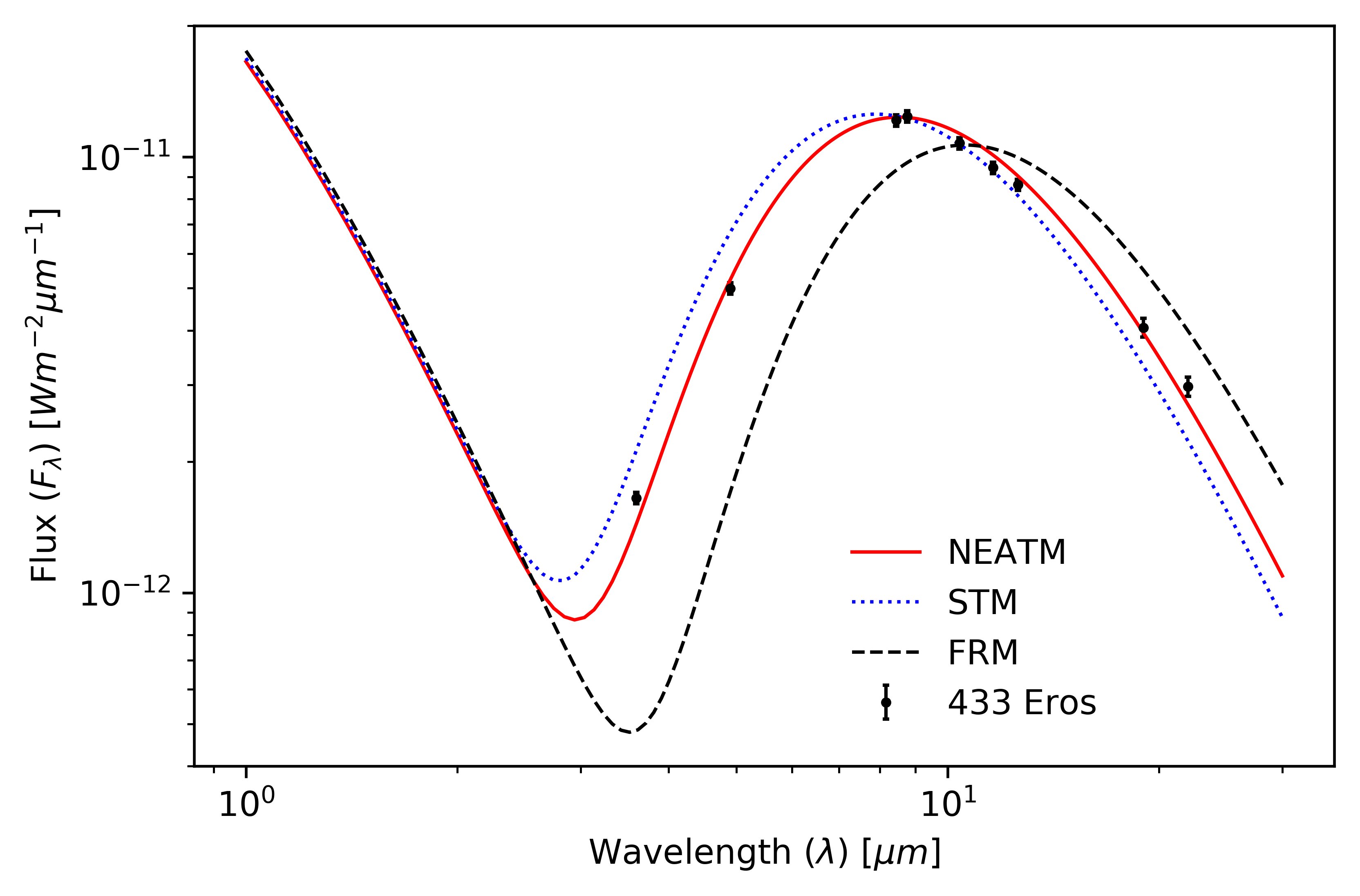
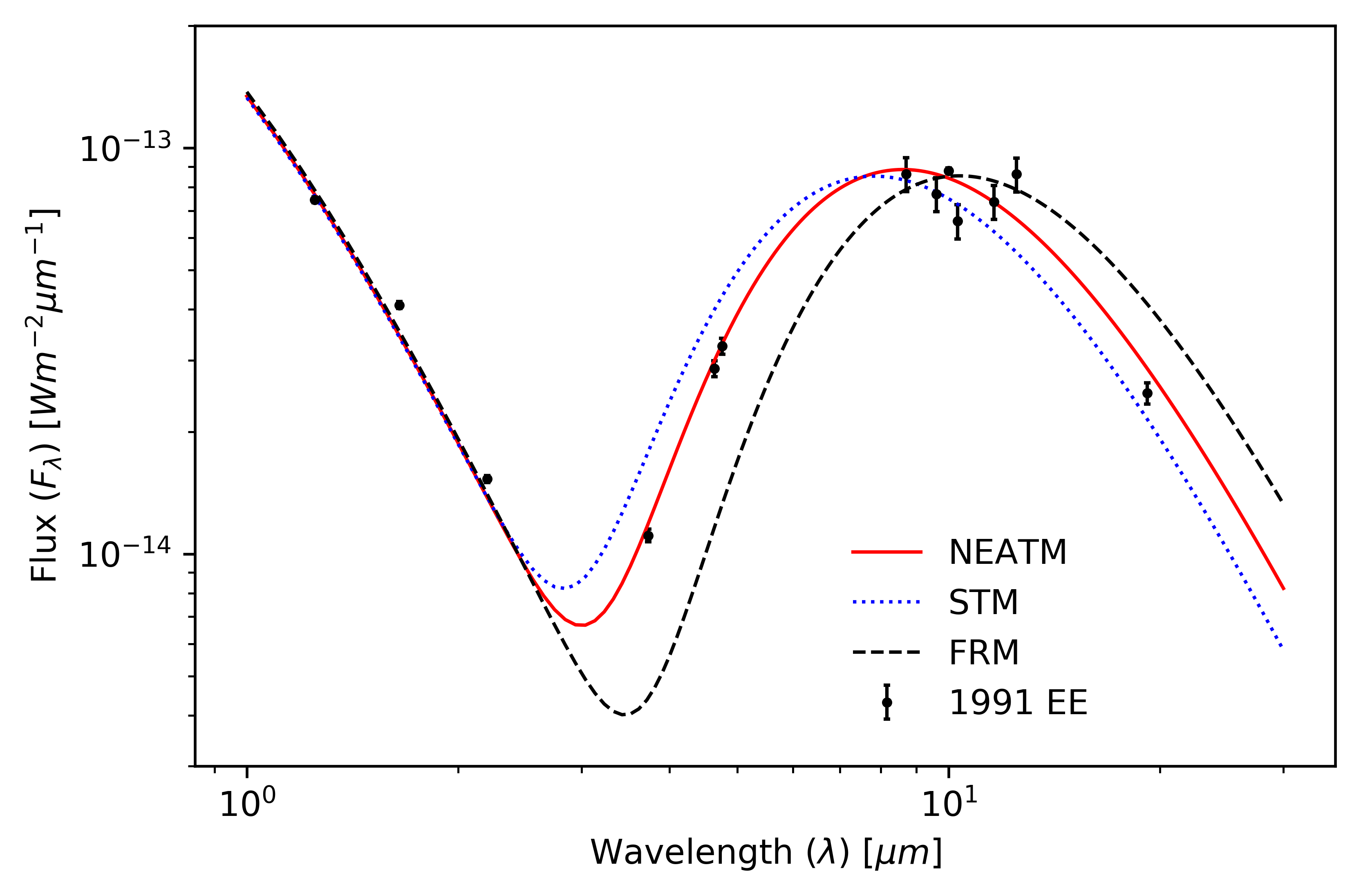
First, we consider the observations of asteroid 433 Eros by Lebofsky & Rieke (1979). We use best-fit model parameters from Harris (1998) and demonstrate in Fig. 5 that ATM produces model fluxes in agreement with measurements. An additional example, with data and analysis for near-Earth asteroid 1991 EE from Harris et al. (1998), also includes and validates the reflected light component, as shown in Fig. 6. Finally, ATM is also validated against NEOWISE results, as described in detail in §4.

Figure 5: Physical model validation using data for 433 Eros (symbols) from Lebofsky & Rieke (1979) and models evaluated using best-fit parameters from Harris (1998). This figure recreates Figure 1a from Harris (1998) and was generated using notebooks/validation/example_Eros.ipynb.

Figure 6: Physical model validation using data for asteroid 1991 EE from Harris et al. (1998). This figure recreates Figure 3 from Harris et al. (1998) and was generated using notebooks/validation/example_1991EE.ipynb.

2.4 The Impact of Missing Bands on Best-fit Parameters

Our validation discussion in §2.3.1 was based on synthetic data for all four WISE bands. The WISE effective bandpass wavelengths are well spaced to provide simultaneous constraints on $T_{1}$, $D$ and $\epsilon_{W1W2}$, given a sufficient number of observations. We have shown above that fitting precision deteriorates as $\epsilon_{W1W2}$ is added as a fitting parameter: with 25 epochs and $\Sigma=0.1$ mag, the uncertainty of best-fit $D$ and $T_{1}$ increases by about a factor of two from 0.92% and 0.52% to 2.5% and 1.1%, respectively (with an uncertainty of 0.012 for $\epsilon_{W1W2}$). Again, these are formal fitting uncertainties when the model is perfectly well known. We now investigate how the precision further deteriorates when only a subset of WISE bandpasses is used in fitting.

When only $T_{1}$ and $D$ are fit, the largest increase in uncertainties, about a factor of two, is seen when the missing bandpass is $W_{1}$. This is because the total flux in the $W_{1}$ bandpass is dominated by the reflected sunlight component and thus it depends very weakly on $T_{1}$. Consequently, $W_{1}$ strongly constrains diameter $D$ in the case of known $\epsilon$ (and thus known albedo). Indeed, when only the $W_{1}$ and $W_{2}$ bandpasses are used, the $T_{1}$ precision worsens by only 50% and the $D$ precision remains unchanged. When only $W_{1}$ and $W_{3}$ are used, there is no appreciable decrease in precision. On the other hand, a combination of the $W_{2}$ and $W_{3}$ bandpasses results in 3 to 4 times larger uncertainties. Somewhat surprisingly, the fitter does not recover the correct parameters when only the $W_{3}$ and $W_{4}$ bandpasses are used. In the latter case, typically the best-fit temperature is under-estimated, while the best-fit size can be larger than the input value by close to a factor of 10. When fitting three parameters ($T_{1}$, $D$ and $\epsilon_{W1W2}$), flux in at least one of the two bluest bandpasses must be available to recover the input parameters. A decrease in precision of less than a factor of two is observed when fitting with three bandpasses as long as the $W_{4}$ band is used in fitting. When the $W_{4}$ data are not used, the fitting precision decreases by about a factor of three compared to the four-bandpass case.

In summary, when only $T_{1}$ and $D$ are fit, even two bandpasses will suffice as long as $W_{1}$ or $W_{2}$ is included, but when $\epsilon_{W1W2}$ is also fit, $W_{4}$ becomes more important than $W_{1}$ and $W_{2}$. However, note the caveat that these conclusions are derived for the somewhat unrealistic case with a lot of observations and small $\Sigma$.

3 Illustration of ATM fitting capabilities

Figure 7: ATM “corner” plot for asteroid (54789) assuming model 5. Here both $\epsilon_{W1}$ and $\epsilon_{W2}$ are free parameters; compare to Figure 8 where an additional constraint $\epsilon_{W1}=\epsilon_{W2}$ is imposed. This figure was generated using notebooks/analysis/single_object_54789.ipynb.

Figure 8: ATM “corner” plot for asteroid (54789) assuming model 4. This model imposes a constraint $\epsilon_{W1}=\epsilon_{W2}$. Compare to Figure 7 where both $\epsilon_{W1}$ and $\epsilon_{W2}$ are free parameters. This figure was generated using notebooks/analysis/single_object_54789.ipynb.

In this section, we illustrate ATM’s capabilities for fitting asteroid spectral energy distributions, with emphasis on the treatment of Bayesian priors when also fitting emissivity, using three well-observed asteroids: (25916), (54789), and (90367). We study how the choices of priors affect the posterior pdf for fitted parameters and we study the resulting biases in point estimates derived from these pdfs (that is, “best-fit parameters”). We consider five different models, where in addition to fitting for asteroid diameter, $D$, and temperature parameter, $T_{1}$, we treat emissivity $\epsilon(\lambda)$ as follows:

• Model 1: $\epsilon(\lambda)=\epsilon_{0}=$ const. and we fit for $\epsilon_{0}$ using a flat prior $0<\epsilon_{0}<1$.

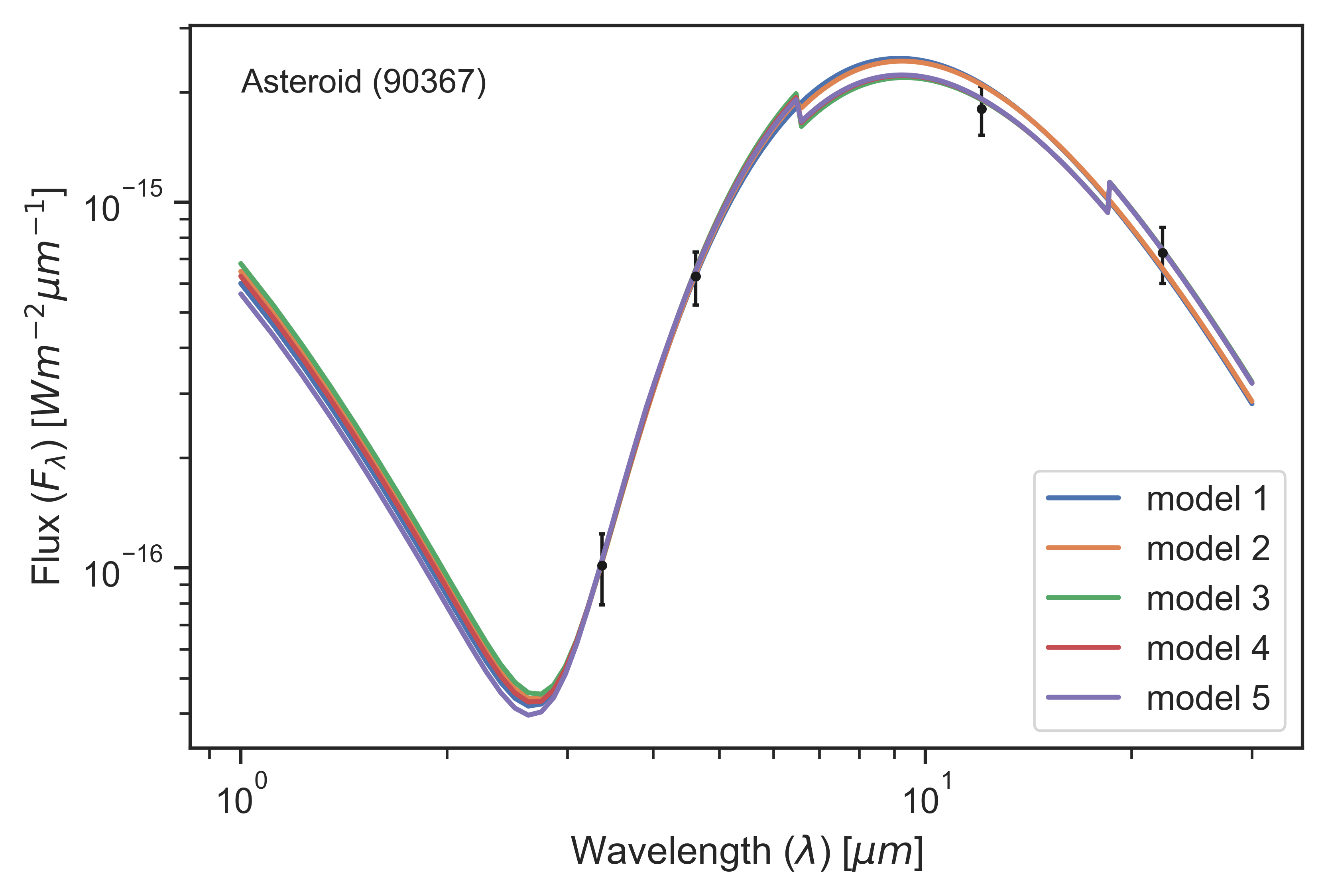
• Model 2: We set $\epsilon_{W3}=\epsilon_{W4}=0.9$ (that is, the prior is the Dirac $\delta$ function) and fit for unknown $\epsilon_{W1}=\epsilon_{W2}=\epsilon_{W1W2}$, where subscripts indicate WISE bands. Here, and in models below, we model $\epsilon(\lambda)$ as a step function, with transition wavelengths between bands at $\lambda_{W1W2}=3.9\,\mu{\rm m}$, $\lambda_{W2W3}=6.5\,\mu{\rm m}$, and $\lambda_{W3W4}=18.5\,\mu{\rm m}$. Note that in SED plots discussed below emissivity $\epsilon_{W1}$ is extrapolated to wavelengths shorter than $\lambda_{W1W2}$, implying a pre-set value for the visual albedo, $p_{V}$. The same is true for emissivity in the most redward band, $\epsilon_{W4}$; it is extrapolated to wavelengths beyond the W4 bandpass for plotting purposes.

• Model 3: We set $\epsilon_{W3}=0.70$ and $\epsilon_{W4}=0.86$, motivated by ensemble analysis presented later in §4.3, and fit for $\epsilon_{W1W2}$.

• Model 4: We set $\epsilon_{W3}=0.80$ and $\epsilon_{W4}=0.98$ and fit for $\epsilon_{W1W2}$. The $\epsilon_{W4}/\epsilon_{W3}$ ratio is the same as in the previous model.

• Model 5: We set $\epsilon_{W3}=0.80$ and $\epsilon_{W4}=0.98$ and fit for $\epsilon_{W1}$ and $\epsilon_{W2}$. Compared to the previous model, here we do not enforce $\epsilon_{W1}=\epsilon_{W2}$ .

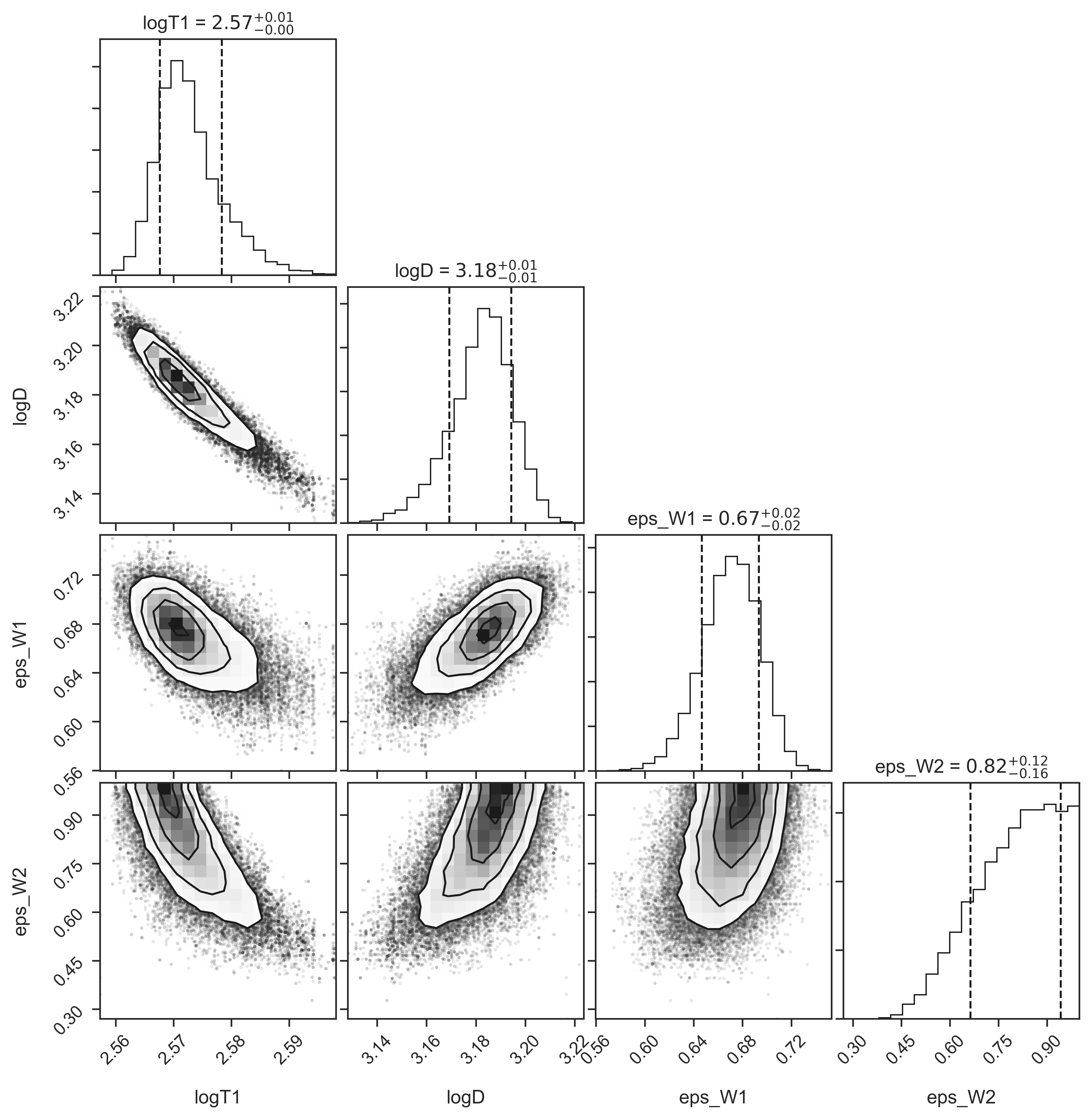
Figure 7 shows the posterior pdf for four fitted parameters in the case of model 5 and asteroid (54789). We have also considered a case where emissivity values in all four bands are free fitting parameters, for a total of six fitted parameters, but concluded that it is sufficient to start the discussion here with model 5. As panels in the bottom row of Figure 7 show, the pdf for $\epsilon_{W2}$ is quite wide and not too dissimilar to its prior, while $D$, $T_{1}$ and $\epsilon_{W1}$ have pdfs that are much narrower than their priors, and with a well defined peak. In other words, $\epsilon_{W2}$ is much less constrained by the data than the other three parameters. This conclusion is also valid for the other two asteroids considered here.

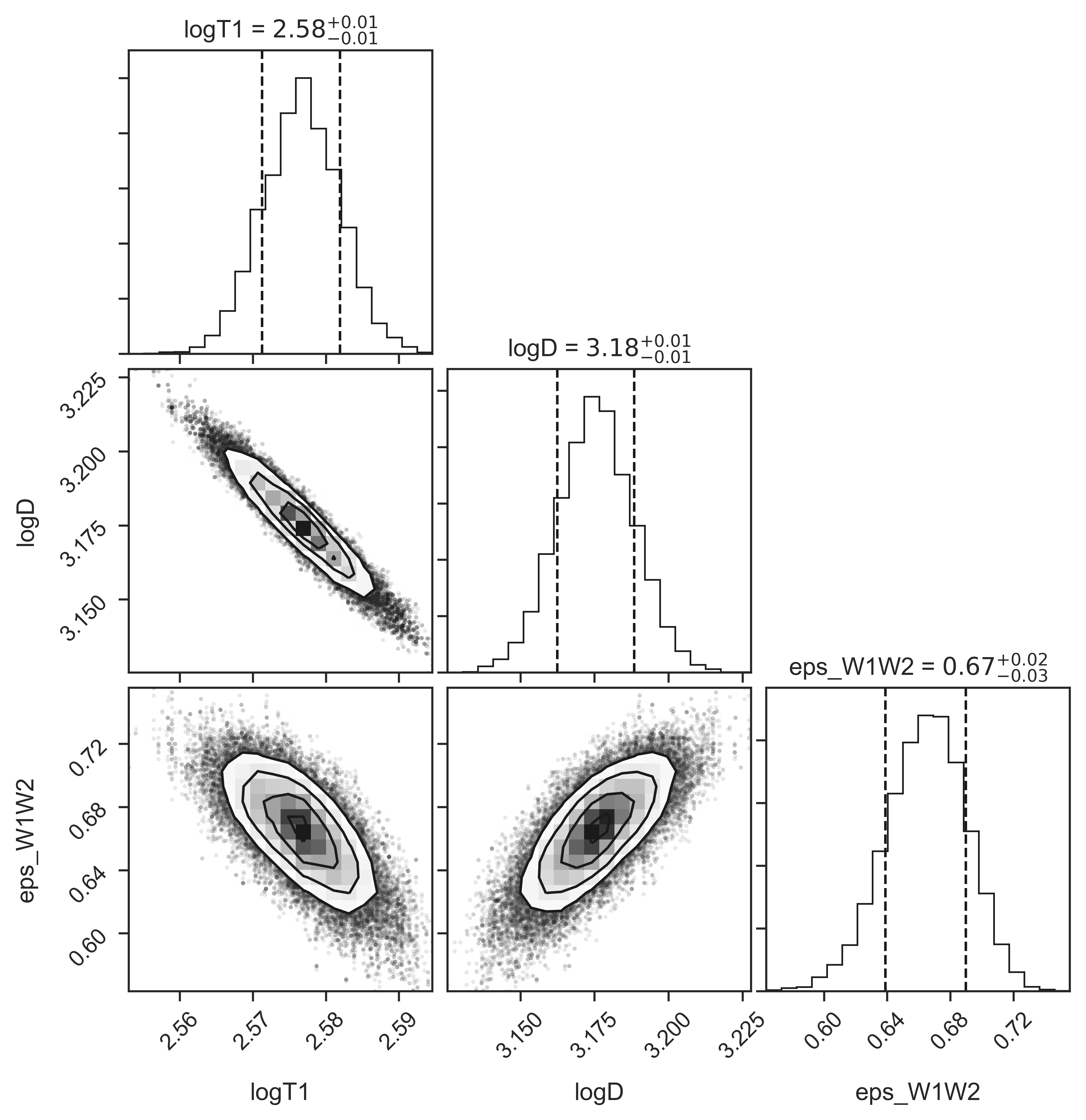
Following the behavior of emissivity inferred from laboratory spectra for different materials, as illustrated in Figure 1 from Myhrvold (2018a), we enforce an additional fitting constraint: $\epsilon_{W1}=\epsilon_{W2}=\epsilon_{W1W2}$ and fit for three free parameters (models 2, 3, and 4). Figure 8 shows the posterior pdf for fitted parameters in the model 4 case. The fitted parameter $\epsilon_{W1W2}$ now has a pdf that is much narrower than its priors and with a well defined peak. The same behavior is observed for the other two asteroids. As a result of this analysis, we conclude that for the robust fitting of these, and other less observed, asteroids, we need to only fit for $\epsilon_{W1W2}$, and not for $\epsilon_{W1}$ and $\epsilon_{W2}$ separately.

There is a remaining question of what to choose for the values of $\epsilon_{W3}$ and $\epsilon_{W4}$ that are not fitting parameters. As Table 1 shows, models 2, 3, and 4 result in values of best-fit $D$ varying by about 10-15%, depending on the chosen values of $\epsilon_{W3}$ and $\epsilon_{W4}$. In addition, adopting $\epsilon(\lambda)=\epsilon_{0}$ and fitting for $\epsilon_{0}$ can result in a change of $D$ as large as 20% (compare model 1 and model 2 for asteroid 54789). This approach also leads to a taxonomy-dependent $D$ bias (systematic uncertainty) because the actual bias depends on detailed deviations of $\epsilon(\lambda)$ from the assumed constant value of $\epsilon_{0}$. We will return to the discussion of optimal choice of $\epsilon_{W3}$ and $\epsilon_{W4}$ in §4.3.

Table 1: The Best-fit NEATM Parameters^a for Asteroids (25916), (54789) and (90367)

Model	log($D$/m)	log($T_{1}$/K)	$\epsilon_{W1}$	$\epsilon_{W2}$	$\epsilon_{W3}$	$\epsilon_{W4}$
Asteroid (25916)
1	3.691	2.587	0.877	=$\epsilon_{W1}$	=$\epsilon_{W1}$	=$\epsilon_{W1}$
2	3.681	2.589	0.874	=$\epsilon_{W1}$	(0.90)	(0.90)
3	3.702	2.585	0.884	=$\epsilon_{W1}$	(0.70)	(0.86)
4	3.684	2.589	0.877	=$\epsilon_{W1}$	(0.80)	(0.98)
5	3.664	2.602	0.902	0.660	(0.80)	(0.98)
Asteroid (54789)
1	3.240	2.558	0.740	=$\epsilon_{W1}$	=$\epsilon_{W1}$	=$\epsilon_{W1}$
2	3.166	2.575	0.653	=$\epsilon_{W1}$	(0.90)	(0.90)
3	3.198	2.571	0.697	=$\epsilon_{W1}$	(0.70)	(0.86)
4	3.175	2.577	0.665	=$\epsilon_{W1}$	(0.80)	(0.98)
5	3.184	2.572	0.672	0.827	(0.80)	(0.98)
Asteroid (90367)
1	3.223	2.580	0.971	=$\epsilon_{W1}$	=$\epsilon_{W1}$	=$\epsilon_{W1}$
2	3.254	2.576	0.972	=$\epsilon_{W1}$	(0.90)	(0.90)
3	3.278	2.572	0.974	=$\epsilon_{W1}$	(0.70)	(0.86)
4	3.261	2.575	0.974	=$\epsilon_{W1}$	(0.80)	(0.98)
5	3.260	2.576	0.976	0.953	(0.80)	(0.98)
(a) The values in parenthesis represent priors.

Figure 9 compares spectral energy distributions for models 1-5 in the case of asteroid (90367). As evident, all models are equally successful in explaining observed fluxes in bands W1 and W2. Models 3, 4 and 5 are more successful than models 1 and 2 in explaining observed fluxes in bands W3 and W4. This improvement is due to the choice $\epsilon_{W4}=1.22\epsilon_{W3}$, instead of $\epsilon_{W4}=\epsilon_{W3}$ for models 1 and 2, and is discussed in detail in §4.3. This model degeneracy implies a bias in best-fit asteroid size in the range 10-20%, as discussed above.

Note that the prediction for reflected flux at wavelengths below $\sim 2\mu{\rm m}$ varies by about 30% due to variation of best-fit $D$ and best-fit $\epsilon_{W1}$, which implies an extrapolated value of $p_{V}$. Nevertheless, a measurement of flux at optical wavelengths could only break the model degeneracy if there were a strong prior reason to believe that emissivity values at optical wavelengths were somehow fully determined by the value of emissivity in the WISE W1 band.

Figure 9: The symbols show the median fluxes and their errors for WISE data for asteroid (90367). The errors include the contribution of assumed variability amplitude of 0.15 mag. The solids line show five NEATM models that differ in chosen priors for emissivity (see text). The best-fit parameters for these models are listed in Table 1. The sharp changes in modeled fluxes at $\lambda_{W2W3}=6.5\,\mu{\rm m}$ and $\lambda_{W3W4}=18.5\,\mu{\rm m}$ is due to a simplistic approximation of emissivity as a function of wavelength as a step function. This figure was generated using notebooks/analysis/single_object_90367.ipynb.

4 Application of ATM to WISE data and comparison with NEOWISE analysis

In this section, we apply ATM to a “gold” sample of $\sim$7,000 best-observed asteroids by WISE. In addition to the best-fit diameter $D$ and characteristic temperature $T_{1}$ for each object, we also obtain best-fit emissivity across bands W1 and W2, $\epsilon_{W1W2}$. We compare ATM best-fit parameters to their values as published by the NEOWISE team, discuss physical implications of the best-fit parameters, and derive an approximate method for estimating $D$ from WISE W3 measurements that doesn’t require model fitting and is applicable to the majority of asteroids with WISE measurements.

4.1 Selection of High-quality WISE Data and Reliable ATM Fits

To cleanly compare ATM best-fit parameters with their values as published by the NEOWISE team, we select a relatively small subsample ($\sim 5$% of the full sample) with the highest quality and quantity of WISE data. Observations of asteroids by WISE were obtained using the same criteria described by NEOWISE papers. The list of observations were obtained from the Minor Planet Center database for observatory code C51. The positions and times were then used to search the WISE All-Sky Single Exposure Level 1b Source catalog using a cone search with radius 10 arcseconds, and an observation time tolerance of $\pm 2$ seconds. The distance from the asteroid to the Sun, distance from the asteroid to WISE, and the phase angle were obtained with the JPL HORIZONS service, using the asteroid designation and observation time. To ensure high quality measurements, we require:

• at least 3 observations with the photometric signal-to-noise ratio of at least 4 in each band, and

• artifact flag = 0 and quality flag = A, B, C, but not U or X.

This set of criteria reduces $\sim 2.5$ million observations of $\sim$150,000 asteroids to $\sim$87,000 observations of 9,672 asteroids (each observation with fluxes measured in up to four WISE bands).

For some objects, measurements still include outliers despite the above quality cuts. We clip outliers using a simple automated iterative algorithm. We first reject all points that are more than 1 mag away from the median magnitude (per band), then fit a straight line to magnitude vs. time relation in each band using the surviving data points, and finally reject all points more than 1 mag away from the best fit line. This outlier clipping reduced the aforementioned 9,672 asteroids down to 7,363 ($\sim$14% of observations at this stage were cut as magnitude outliers). Finally, 4 objects were removed as they had missing assumptions on physical parameter, $G$. The final “gold” sample contains $\sim$ 77,000 observations of 7,359 objects.

For each object, we fit for diameter $D$, characteristic temperature $T_{1}$ and emissivity across the W1–W2 wavelength range, $\epsilon_{W1W2}$. We produced four sets of fits that differ in priors for emissivity across the W3–W4 wavelength range. Following NEOWISE analysis, we adopted $\epsilon_{W3}=\epsilon_{W4}=0.90$ for the first set. Informed by discrepancies between the observed and modeled distributions of objects in the W3-W4 vs. W2-W3 color-color diagram (see below for detailed discussion), for the other three sets we adopted $(\epsilon_{W3},\epsilon_{W4})$ = (0.80, 0.98), (0.76, 0.93) and (0.70, 0.86).

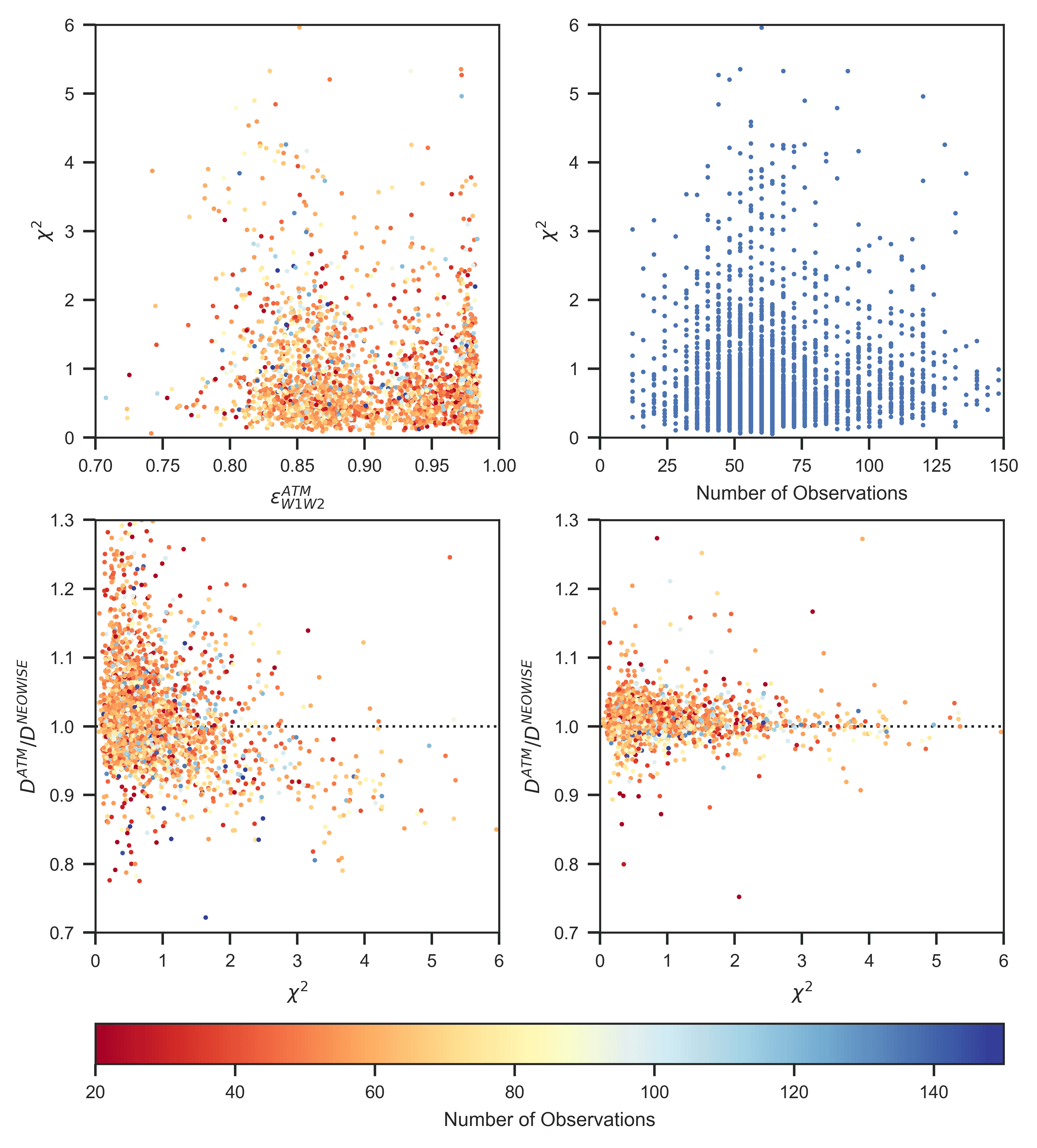
The top right panel in Figure 10 shows the distribution of $\chi^{2}$ per degree of freedom as a function of the total number of data points in all 4 bands. The computation of $\chi^{2}$, as well as fitting, assumes an intrinsic scatter due to variability of $\Sigma=0.15$ mag (see eq. 9). The distribution of $\chi^{2}$, with a mode at unity, validates this choice. There is no correlation of the $\chi^{2}$ distribution with the number of data points; typically, there are $\sim$50 measurements per object.

Figure 10: The top left panel shows the $\chi^{2}$ per degree of freedom vs. $\epsilon_{W1W2}$ diagram for asteroids that pass initial quality cuts (see §4.1), have NEOWISE fit code “DVBI” and have at least 3 observations in each of the four WISE bands. The best-fit $\chi^{2}$ and emissivity $\epsilon_{W1W2}$ were obtained using ATM. The symbols are color-coded using the total number of data points, according to the legend below the panel. The top right panel shows the $\chi^{2}$ vs. the total number of data points diagram. The bottom panels show the ratios of the best-fit diameter (left) and $\epsilon_{W1W2}$ (right) obtained by ATM and the 2016 NEOWISE release values vs. $\chi^{2}$, color-coded the same way as in the top left panel. This figure was generated using notebooks/analysis/analysis.ipynb.

4.2 Comparison to NEOWISE Fits

To compare our best-fit parameters to those obtained by the NEOWISE team, we match objects from our dataset to objects from the 2016 Planetary Data System version of the NEOWISE Diameters and Albedos database (Mainzer et al., 2016), hereafter “NEOWISE values”. For this initial comparison, we also require NEOWISE fit code “DVBI” and at least 3 observations in each of the four WISE bands, yielding a comparison sample of 2,807 asteroids. We selected only the NEOWISE results for each asteroid that used the most data points as some asteroids had multiple fitting results under the same fit code. The ratio of best-fit ATM and NEOWISE values vs. $\chi^{2}$ for diameter $D$ and emissivity $\epsilon_{W1W2}$ is shown in the bottom panels in Figure 10. As evident, there is a good agreement between the two sets of best-fit parameters.

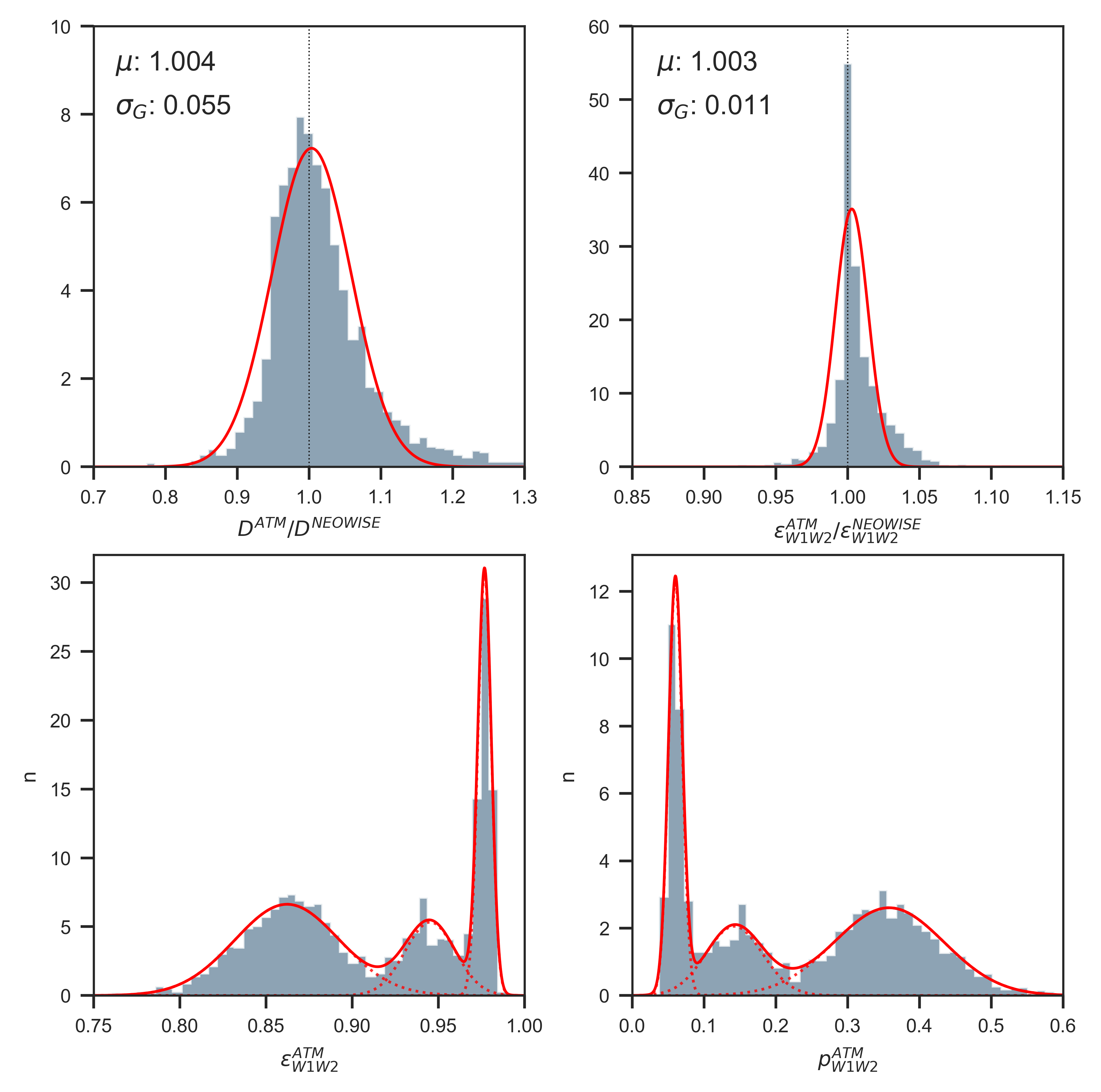
A more quantitative comparison is shown in the top two panels in Figure 11, for the fitting case with $\epsilon_{W3}=\epsilon_{W4}$ = 0.90. Both the best-fit diameters and emissivity agree on average to within 0.4%, with a scatter of 5.5% for diameters and 1.1% for emissivity. Plausible reasons for the scatter include different outlier rejection algorithms, different treatments of Kirchhoff’s law (for a detailed discussion, see Myhrvold 2018a), and how ATM accounts for intrinsic variability, although we cannot exclude other causes (e.g., a slight error in the quadrature formula for the W3 band, see Appendix A for details). Whatever the reason, the discrepancies are encouragingly small.

Our ATM results faithfully match the tri-modal distribution of $\epsilon_{W1W2}$ emissivity discovered by Masiero et al. (2014). The two bottom panels in Figure 11 show the resulting distributions of emissivity and corresponding albedo based on ATM results. The parameters of a best-fit 3-component Gaussian mixture model are listed in Table 2. Note that the fractions of three components listed in Table 2 (20%, 30% and 50%) are not corrected for the various sample selection effects.

This tri-modality is related to taxonomic classes; according to Masiero et al. (2014) the low and high p_W1W2 albedo peaks correspond to the low and high visible albedo groups observed previously (C/D/P and S groups, respectively), while the intermediate albedo peak corresponds to intermediate visible albedo values that are blended with the high albedo objects in visible albedo distributions.

Figure 11: The top panels show histograms of the ratios of the best-fit diameter (left) and $\epsilon_{W1W2}$ (right) ATM and the 2016 NEOWISE release values, for 2,656 asteroids with $\chi^{2}<3$ (ATM) and at least 28 observations. The red lines are single Gaussian fits, with their mean and standard deviation shown in each panel (e.g., ATM matches NEOWISE fits with a bias of 0.3% and a scatter of 6.5%, though note the distribution is leptokurtic). The bottom panels show distributions of emissivity $\epsilon_{W1W2}$ (left) and corresponding albedo (right) for the same objects. The solid lines show best-fit 3-component Gaussian mixtures (fit to individual data points rather than to histograms which are shown only for illustration). The best-fit parameters are listed in Table 2. This figure was generated using notebooks/analysis/analysis.ipynb.

Table 2: The Best-fit Parameters for Emissivity and Albedo Distributions

Quantity	fraction1	$\mu_{1}$	$\sigma_{1}$	fraction2	$\mu_{2}$	$\sigma_{2}$	fraction3	$\mu_{3}$	$\sigma_{3}$
Emissivity $\epsilon_{W1W2}$	0.299	0.977	0.004	0.195	0.945	0.015	0.506	0.862	0.030
Albedo pW1W2	0.296	0.060	0.010	0.203	0.142	0.039	0.501	0.358	0.077

4.3 Understanding ATM Best Fits

Despite good agreement between ATM and NEOWISE fitting results, there are statistical problems with best-fit models when $\epsilon_{W3}=\epsilon_{W4}$ = 0.90: the per-band magnitude residual distributions for all objects are offset from zero by 0.1–0.2 mag in most bands. These offsets indicate that the thermal models used are not fully capable of explaining WISE data. The distributions of observed objects in WISE color-color diagrams offer an efficient way to study possible causes of model deficiencies. We note that the use of a full sample to constrain priors for individual objects is known as Hierarchical Bayesian modeling (e.g., see Chapter 5 in Ivezić et al. 2014).

For each object, we compute the median observed magnitudes in each WISE band and the median observed colors. The resulting color-color diagrams are shown in Figure 12. The position along the model sequences in the W3-W4 vs. W2-W3 color-color diagram (see the bottom right panel in Figure 12) is by and large controlled by the asteroid-Sun distance $r$, while both $r$ and emissivity $\epsilon_{W1W2}$ (or, equivalently, albedo) determine the position in the W2-W3 vs. W1-W2 color-color diagram (bottom left panel). Note the three clearly delineated observed sequences in this diagram. Their finite width is influenced by both the distribution of $\epsilon_{W1W2}$ values, and the distribution of observational phase angles (increase in $\epsilon_{W1W2}$ and/or phase angle moves model sequences from the bottom left to the top right). Note also that the W2-W3 and W3-W4 colors become redder as $r$ increases, while the W1-W2 color becomes redder for decreasing $r$ (because of the increasing relative contribution of the blue reflected component).

Figure 12: The symbols correspond to 2,656 asteroids with $\chi^{2}<3$ (ATM) and at least 28 WISE observations. Except for the top right panel, symbols are color-coded according to the median asteroid-Sun distance, $r$. The top right panel shows the variation of W2-W3 color with $r$. The three solid lines in each panel are model tracks produced with three fixed pairs of characteristic temperature, $T_{1}$, and emissivity across the W1 and W2 wavelength range, $\epsilon_{W1W2}$ (0.98, 406 K; 0.95, 399 K; 0.86, 391 K; for black, red and blue tracks, respectively). The position along each track is controlled by the asteroid-Sun distance (models are computed for the range 1.5–5.5 AU). Colors do not depend on the object size and distance from the observer; however, the position in the W1 vs. W1-W2 color-magnitude diagram (top left) depends on both of these quantities and model tracks assume a fiducial asteroid diameter of 10 km at a distance of 1 A.U. Emissivity across the W3 and W4 wavelength range, parameterized as $\epsilon_{W3}$ and $\epsilon_{W4}$, controls the placement of model tracks in the W3-W4 vs. W2-W3 color-color diagram. The model tracks shown by solid lines are computed using $\epsilon_{W3}=0.80$ and $\epsilon_{W4}=0.98$. Model tracks shown by dashed lines correspond to the usually adopted values $\epsilon_{W3}=\epsilon_{W4}=0.90$, and are strongly ruled out by the data distribution in the W3-W4 vs. W2-W3 color-color diagram. This figure was generated using notebooks/analysis/analysis.ipynb.

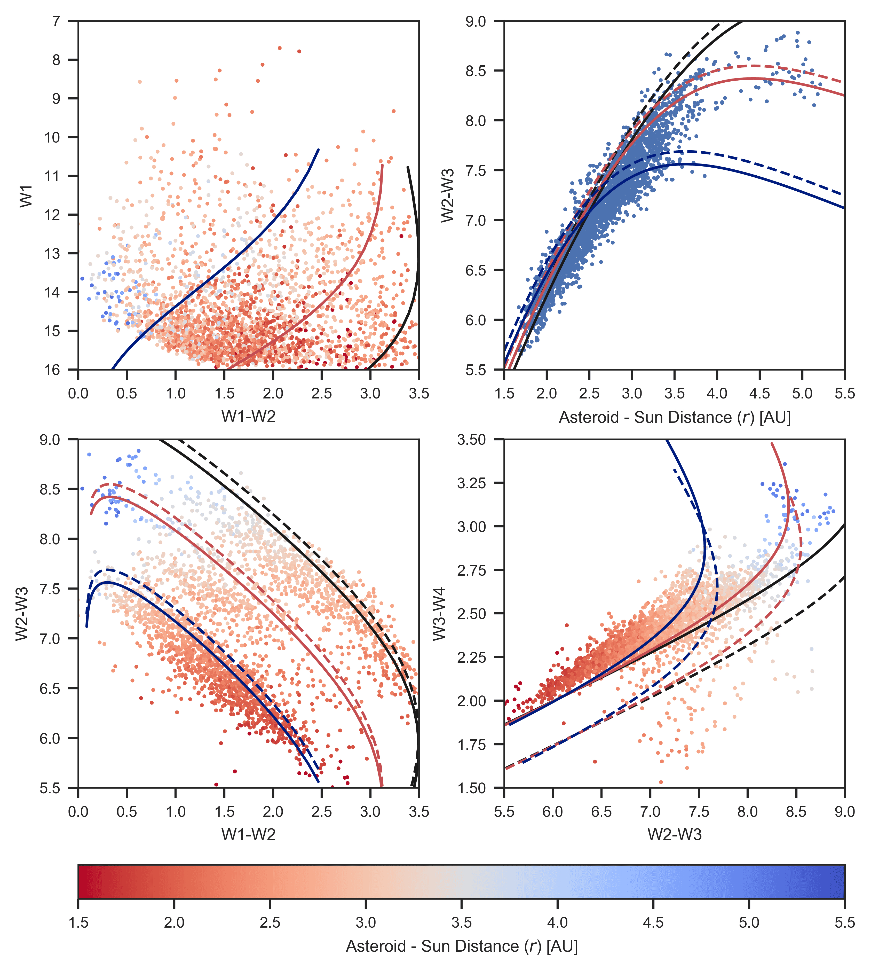
The placement of model tracks in the W3-W4 vs. W2-W3 color-color diagram is controlled by emissivity across the W3 and W4 wavelength range, parameterized as $\epsilon_{W3}$ and $\epsilon_{W4}$, while the position along the tracks is controlled by the asteroid’s temperature (itself controlled by $T_{1}$ and the asteroid-Sun distance). The three model tracks shown by dashed lines correspond to $\epsilon_{W3}=\epsilon_{W4}=0.90$, and are strongly ruled out by the data: they don’t overlap the majority of data points.

A small fraction of data points (about 3%) with very blue W3-W4 colors could be, at least in principle, either measurement outliers, or interesting objects with unusual $\epsilon_{W3}$ and $\epsilon_{W4}$ values. However, all of them are extremely bright in W3 (W3$<$1.8) and essentially represent the top 3% brightest sources. Hence, it is likely that their peculiar behavior in the W3-W4 vs. W2-W3 color-color diagram is simply due to overestimated W3 flux by about 0.5 mag. This conclusion is consistent with the recently reported flux corrections for saturation in the W3 band by Wright et al. (2018).

The only way to move model tracks to reach the data distribution is to assume $\epsilon_{W4}>\epsilon_{W3}$. After some experimentation, we adopted $\epsilon_{W4}\approx 1.22\epsilon_{W3}$. The required scale of $\epsilon$ is only set when W1 data is added because the W1 band includes a significant contribution from the reflected light component (proportional to $(1-\epsilon)D^{2}$, rather than to $\epsilon D^{2}$ for thermal emission component, as discussed earlier).

We investigated three pairs of values: $(\epsilon_{W3},\epsilon_{W4})$ = (0.80, 0.98), (0.76, 0.93) and (0.70, 0.86). All three pairs produce model tracks in Figure 12 that are in a much better agreement with data than $\epsilon_{W3}=\epsilon_{W4}=0.9$. The model tracks could be moved further to completely overlap the data distribution by adopting $\epsilon_{W4}\approx 1.34\epsilon_{W3}$ (e.g., $\epsilon_{W3}=0.73,\epsilon_{W4}=0.98$). We leave detailed investigation of such models to future work.

While in all three cases the agreement between the data and the models in color-color diagrams is essentially unchanged, the values of best-fit diameters change in inverse proportion to the values of $\epsilon$. Relative to the best-fit diameters for $(\epsilon_{W3},\epsilon_{W4})$ = (0.80, 0.98) case, which on average agree with the NEOWISE values to better than 1%, the sizes for (0.76, 0.93) case are on average 4% larger, and 10% larger for (0.70, 0.86) case. Note that best-fit diameters scale with $\epsilon$ faster ($\propto\epsilon^{-0.7}$) than the naively expected $1/\sqrt{\epsilon}$ due to non-linear fitting effects. We chose $(\epsilon_{W3},\epsilon_{W4})$ = (0.80, 0.98) for the rest of analysis here because of agreement with the NEOWISE values but we emphasize that these fiducial diameter values could easily have a systematic error exceeding 10% simply due to incorrect priors for $\epsilon_{W3}$ and $\epsilon_{W4}$. It is plausible that these biases could be larger for the $\epsilon_{W4}\approx 1.34\epsilon_{W3}$ case.

This simple analysis illustrates how data can constrain model parameters, and also justifies our updated choice of priors for $\epsilon_{W3}$ and $\epsilon_{W4}$. We now proceed with the analysis of best-fit model parameter distributions, their relationship to data properties, and derive an approximate size estimator that can be applied to the majority of objects in WISE sample.

Figure 13: The symbols correspond to 2,656 asteroids with $\chi^{2}<3$ (ATM) and at least 4 observations in each band. The top left panel shows the W2-W3 vs. W1-W2 color-color diagram, with symbols color-coded by the best-fit values of $\epsilon_{W1W2}$. The three observed sequences clearly correspond to different taxonomic groups. The top right panel shows that the W2-W3 color is by and large controlled by the asteroid-Sun distance, $r$, while characteristic temperature, $T_{1}$, has only a secondary influence due to its small dynamic range. The bottom left panel shows a weak correlation between albedo (or equivalently $\epsilon_{W1W2}$) and $T_{1}$ (the albedo distribution is tri-modal, see the bottom right panel in Fig. 11). The bottom right panel shows a correlation of “absolute” magnitude (corrected for the asteroid size and asteroid-observer distance) with $r$. The preponderance of low-albedo objects at large $r$ reflects the structure of the asteroid belt. This figure was generated using notebooks/analysis/analysis_W3.ipynb.

4.4 An Approximate Single-band W3-based Size Estimator

The availability of WISE measurements varies greatly with bandpass and only a small minority of asteroids have data in all four bands. The majority of asteroids have data only in W3 and W4 bands, or in the W3 band alone. The best coverage is in W3 band. The NEOWISE team developed an elaborate set of different modeling approaches depending on which bands have data (for a concise summary, see §3 in Myhrvold 2018b). Here we propose a much simpler two-step calibration and modeling scheme:

1. In the first step, size, temperature parameter and infrared emissivity $\epsilon_{W1W2}$ are fit for several thousand asteroids with WISE data in all four bands. The subset of these objects with direct size measurements is used to calibrate and validate NEATM model parameters and priors (not done here but implicitly used since the NEOWISE team validated their best-fit sizes using about 100 such objects, which we reproduce here with a subpercent bias).

2. In the second step, only W3 measurements are used to estimate the object’s size, and the method is calibrated and validated using the four-band sample from the first step.

Hence, for studies requiring large samples of objects with size estimates (e.g., tens of thousands), the second step can provide a uniform dataset with well understood random and systematic size uncertainties from the 4-band sample, which is in turn calibrated using objects with direct size measurements.

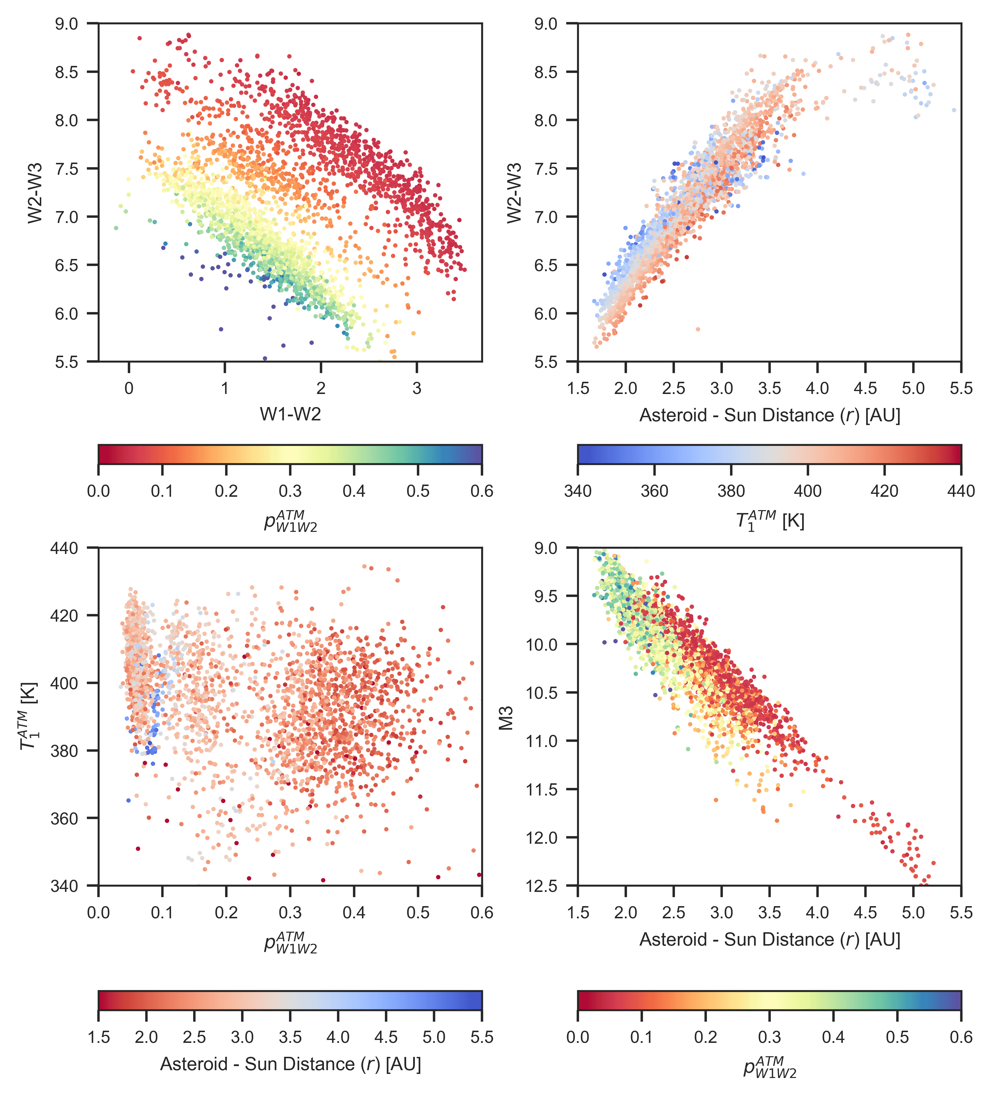
The top left panel in Figure 13 shows the distribution of objects in the W2-W3 vs. W1-W2 color-color diagram, with symbols coded by the near-IR albedo derived from the best-fit emissivity $\epsilon_{W1W2}$. We use model with $\epsilon_{W3}=\epsilon_{W4}=0.9$ because of direct comparison with NEOWISE results further below. As evident, the three sequences displayed by data distribution are related to albedo, and to its tri-modal distribution shown in Figure 11. As was demonstrated in Figure 12, the position along each sequence is by and large controlled by the asteroid temperature, which itself is controlled by the best-fit $T_{1}$ and asteroid-Sun distance. These relations are illustrated in the top right panel in Figure 13. The distribution of best-fit $T_{1}$ is rather narrow and only weakly correlated with near-IR albedo, as shown in the bottom left panel in Figure 13.

As expected from eq. 4, $T_{1}$ does not strongly depend on asteroid-Sun distance. Given this independence and a rather narrow distribution of $T_{1}$, it is possible to derive an approximate but relatively precise predictor for the asteroid flux, given the observing geometry (asteroid-Sun distance, $r$, and asteroid-observer distance, $\Delta$). We first define a “pseudo-absolute” magnitude that accounts for the dependence of observed flux on asteroid size ($\propto D^{2}$) and its distance from the observer ($\propto\Delta^{-2}$),

$$M=W+5\,\log\left(\frac{D}{\rm km}\right)-5\,\log\left(\frac{\Delta}{\rm A.U.}\right).$$ (11)

The variation of this “pseudo-absolute” magnitude constructed using WISE W3 band data with asteroid-Sun distance is shown in the bottom right panel in Figure 13. At a given asteroid-Sun distance, the distribution of $M3$ is rather narrow because both $T_{1}$ and $\epsilon_{W3}$ distributions are narrow.

A linear fit to $M3$ as a function of asteroid-Sun distance,

$$M3=0.863\,\left(\frac{r}{\rm A.U.}\right)+7.859.$$ (12)

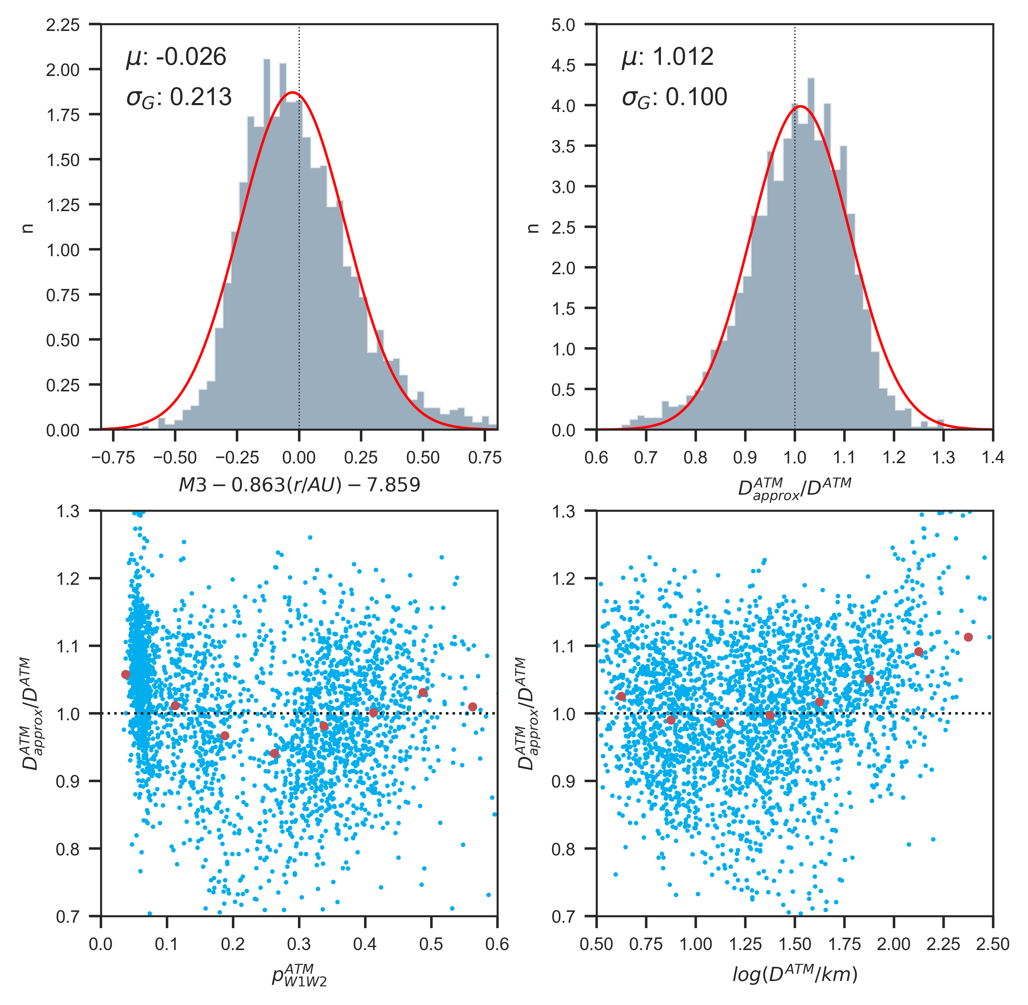
is adequate and matches observed values with a scatter of 0.21 mag, as shown in the top left panel in Figure 14. Using this fit and the definition of $M3$ given by eq. 11, we derive an approximate estimator for asteroid size

$$5\,\log\left(\frac{D_{approx}}{\rm km}\right)=7.589+0.863\,\left(\frac{r}{\rm A.U.}\right)-W3+5\,\log\left(\frac{\Delta}{\rm A.U.}\right).$$ (13)

As shown in the top right panel in Figure 14, this single-band estimator matches best-fit diameters based on data in all four bands with a scatter of only about 10%. This scatter is primarily due to scatter in unknown $T_{1}$ and $\epsilon_{W3}$ around their typical values implicitly assumed in eq. 13. For the same reason, systematic errors are correlated with albedo, at about the 5% level as shown in the bottom left panel in Figure 14. We also find a bias of about 10% for the largest objects (bottom right panel).

Figure 14: The top left panel shows a histogram of residuals after a straight line is fit to the “absolute” magnitude vs. the asteroid-Sun distance relationship shown in the bottom right panel in Fig. 13. The histogram in the top right panel shows the distribution of the ratio of an approximate asteroid diameter estimate based on W3 measurements alone and the best-fit ATM values based on all four WISE bands. The red lines are single Gaussian fits, with their mean and standard deviation shown in each panel. Note that single-band estimates match 4-band estimates with a scatter of 10% and a bias of 1% (this scatter is not dominated by the formal random uncertainties of single-band diameter estimates). The bottom two panels illustrate systematic uncertainty in this approximate estimate as a function of albedo and diameter. The large symbols are the median values for bins along the horizontal axis. This figure was generated using notebooks/analysis/analysis_W3.ipynb.

The usefulness of the approximate size estimator given by eq. 13 is primarily that it can be applied to a much larger sample of objects than the 4-band sample discussed above. We computed the median W3 magnitude for 128,660 unique objects, that also have NEOWISE size estimates, using about 2.3 million W3 measurements. The formal size uncertainties based on scatter in observed W3 magnitudes and an intrinsic variability of 15% are in the range 2-6% for objects with W3 $<8$ and about 10% at the sample faint limit (W3$\sim$10).

The two size estimators are compared in Figure 15, as a function of the NEOWISE fit code. They agree on average with a scatter of about 10%, and without appreciable biases for the high data quality “DVBI” subsample (as expected, as this subsample is closely related to the training sample). However, the two by far largest subsamples, “DVB-” and “DV–” show biases exceeding 10%, and these biases have different behavior for different fit codes. Given that we apply a single estimator, it is likely, although not certain, that biases are introduced by the NEOWISE size estimator. As a possible clue, we find that the bias increases with the formal uncertainty in median W3 magnitude.

Figure 15: The panels show the ratio of W3-based size estimate and the 2016 NEOWISE estimate for subsamples of objects selected by their NEOWISE fitting code and the number of observations (symbols in top two panels and contours in bottom two panels due to much larger subsamples), as a function of the median observed W3 magnitude. The large symbols show the median values of size ratio in bins of W3. The three numbers in each panel list the subsample size, the median value of size ratio, and its robust (interquartile based) standard deviation. Top panels show “DVBI” sample, without (left) and with (right) a limit on the minimum number of observations in all four WISE bands. Bottom panels show “DVB-” subsample (left) and “DV–” subsample (right), with a limit on the minimum number of observations as shown next to the label. This figure was generated using notebooks/analysis/analysis_W3.ipynb.

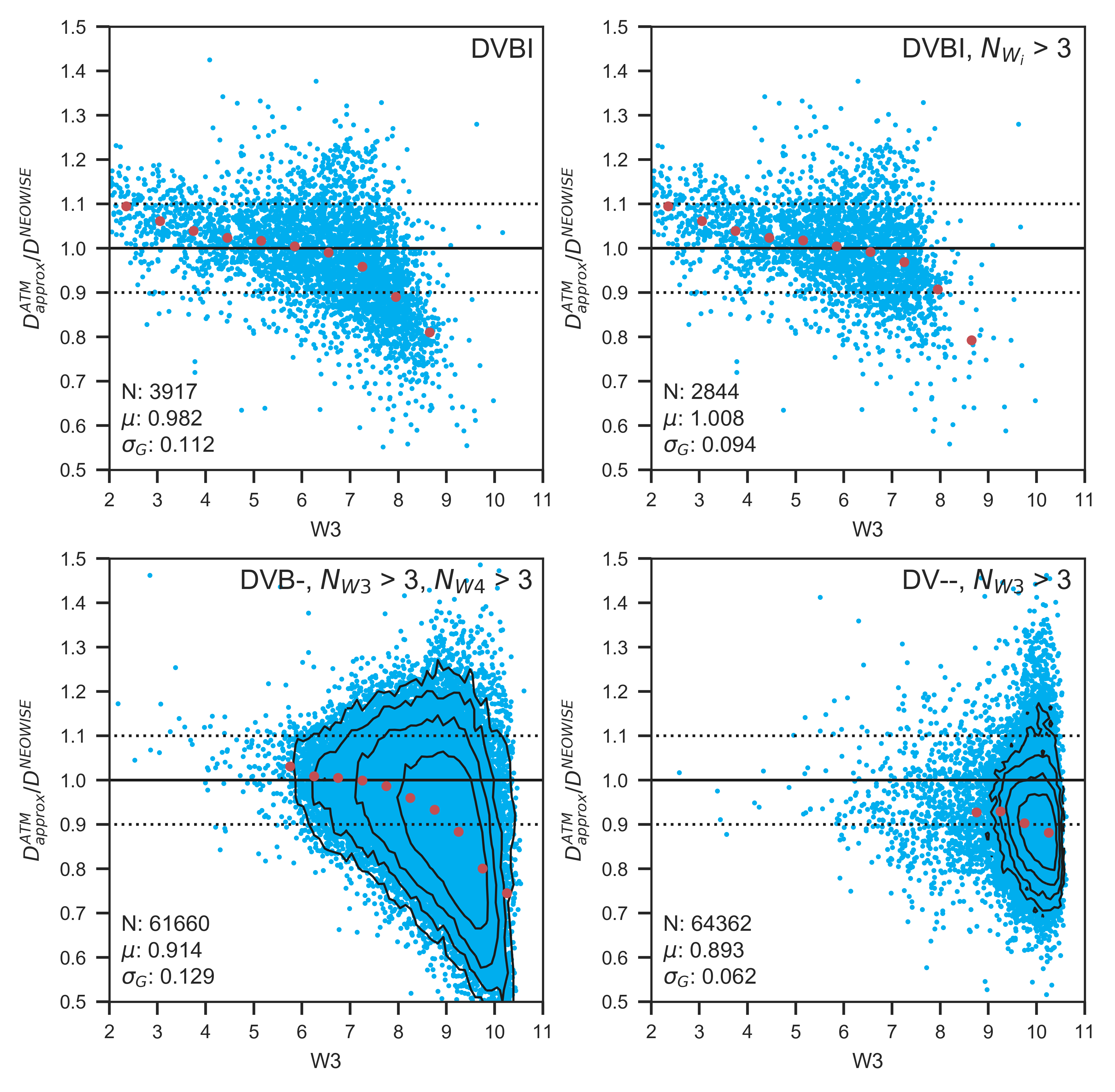
We note that because of a strong correlation between the median W3 flux and asteroid size (because of the finite dynamic range of observed distances), the biases with respect to the median W3 flux propagate to biases with respect to the object size and thus may introduce biases when estimating size distributions.

5 Comparison of WISE-based model parameters and SDSS data

In this section, we match the “gold” sample of 7,359 best-observed asteroids from the WISE dataset (see §4.1 for selection criteria) to asteroids with optical observations listed in the Sloan Digital Sky Survey Moving Object Catalog (hereafter SDSSMOC; Ivezić et al. 2001, 2002; Jurić et al. 2002; Parker et al. 2008). Following Mainzer et al. (2012), we aim to study correlations between optical and infrared properties, such as colors and albedo. In addition, we quantitatively explore the color vs. albedo correlation and develop an approximate method to estimate asteroid size from optical data alone.

The 4th SDSSMOC release lists astrometric and photometric data for 471,569 moving objects observed by SDSS prior to March 2007. Of those, 220,101 objects are linked to 104,449 unique objects with orbits. A match based on object designation to 7,359 objects with WISE-based fits yields 1,574 objects.

In the remainder of the analysis here, we use optical absolute magnitude, $H$, based on SDSS measurements (field 47 in SDSSMOC) because it represents an observationally uniform dataset, and because the values obtained from Minor Planet Center were found to have errors (both biases and random scatter) at the level of a few tenths of magnitude (for detailed discussion, see §2.3 in Parker et al. 2008). However, we note that the net offset between the SDSS and MPC values of $H$, reported by Parker et al. (2008), disappears when using the June 2018 version of the MPC catalog MPCORB.DAT, and the scatter is reduced to 0.22 mag.

5.1 Estimates of optical albedo from WISE-based best-fit sizes

Using SDSS-based absolute magnitude $H$ and WISE-based best-fit size $D$, we estimate optical albedo using eq. 6, repeated here for convenience

$$p_{V}=\left({1329\,{\rm km}\over D}\right)^{2}\,10^{-0.4H}.$$ (14)

This estimate implies that $p_{V}$ is a free fitting parameter whose prior is decoupled from emissivity and albedo values at IR wavelengths probed by WISE. If some prior data implied a strong emissivity/albedo relationship across the entire probed wavelength range (e.g., when assuming a constant unknown value of emissivity $\epsilon$), then a joint fit would be more appropriate and $D$ would be constrained by both optical and infrared data. Given that our knowledge of the emissivity vs. wavelength curve for individual objects is usually poor, and that observed emissivity values span a much smaller dynamic range than albedo values, it is better to first estimate size at wavelengths where thermal emission dominates total observed flux, and then use that best-fit size to estimate albedo at wavelengths were reflected light dominates total observed flux.

5.2 Optical albedo-color correlation

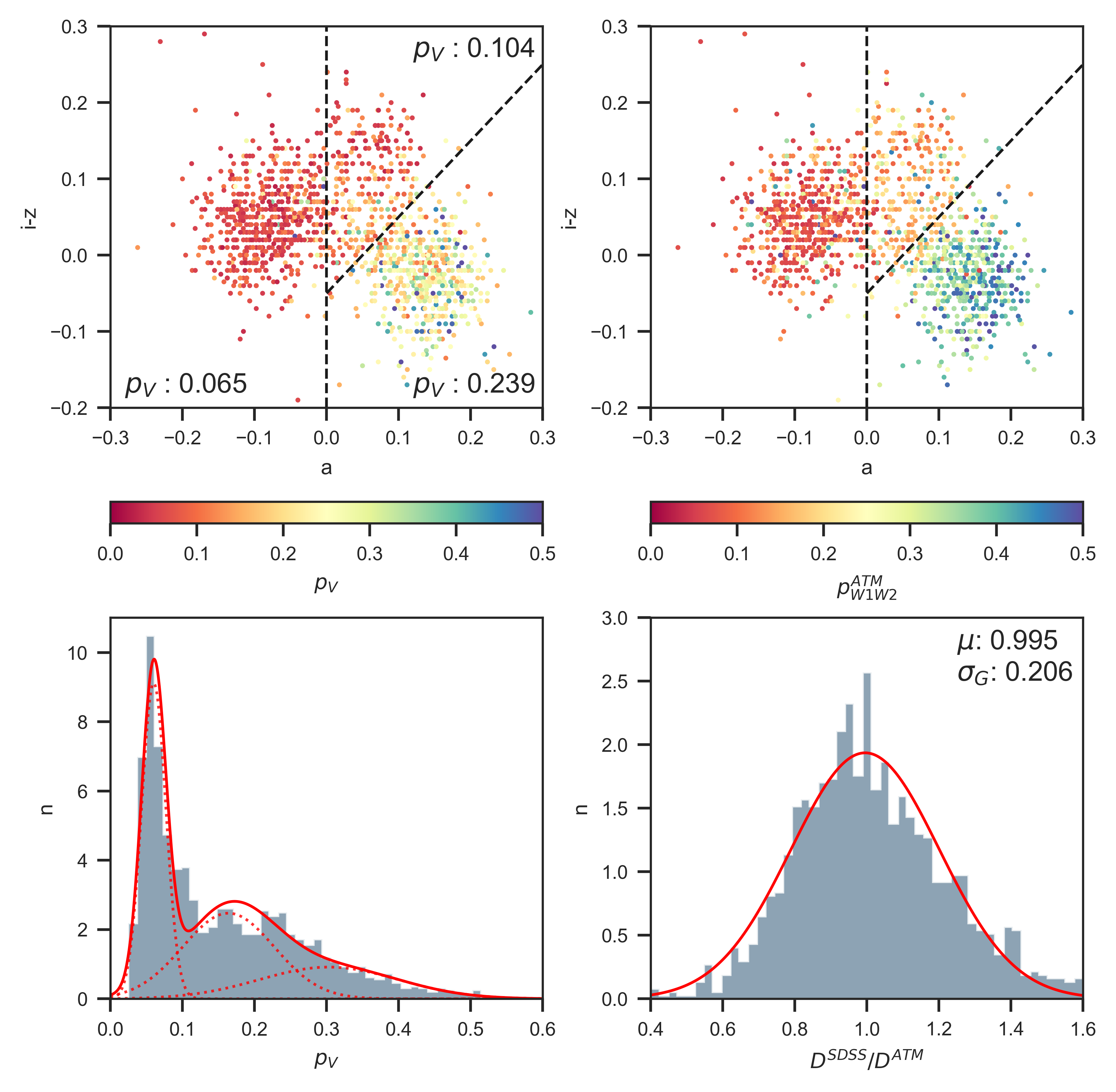
Following Figure 5 from Mainzer et al. (2012), the top two panels in Figure 16 show the SDSS $a$ color vs. $i-z$ color-color diagram, with symbols color coded using the V band albedo from eq. 14 (left) and IR albedo derived from best-fit $\epsilon_{W1W2}$ (right). The $a$ color is the first principal axis for the asteroid distribution in the SDSS $r-i$ vs. $g-r$ color-color diagram, defined as (Ivezić et al., 2001)

$$a=0.89(g-r)+0.45(r-i)-0.57,$$ (15)

and enables easy separation of C type asteroids ($a<0$) from S type asteroids ($a>0$).

As discussed by Mainzer et al. (2012), the addition of IR albedo improves the definition of taxonomic regions, and presumably of subsets of asteroids with different optical albedo distributions, in the optical $r-i$ vs. $g-r$ color-color diagram. Motivated by the morphology of diagrams shown in the top two panels, in addition to the $a=0$ separator, we add the line $i-z=a-0.05$ and separate the sample intro three subsamples. The median optical albedo for these subsamples is listed in the top left panel in Figure 16. The medians and robust standard deviations are listed in Table 3.

Table 3: The median and robust standard deviation for the visual albedo, $p_{V}$.

Color-selected sample	Median	St.dev.a
$a<0$	0.065	0.029
$a>0$ & $i-z>a-0.05$	0.104	0.065
$a>0$ & $i-z<a-0.05$	0.239	0.089

Figure 16: The top panels show the $a$ vs. $i-z$ SDSS color-color diagram, where a color is defined as $a=0.89*gr+0.45*ri-0.57$ (Ivezić et al., 2001), for 1,644 asteroids from SDSS MOC4 catalog that also have WISE-based distances and IR albedo estimated with ATM. The symbols are color-coded by WISE-based IR albedo (right) and by V-band albedo (left) obtained using WISE-based diameter and SDSS-based absolute magnitude. The vertical dashed line shows the separation between C and S taxonomic classes from Ivezić et al. (2001), while the solid line is a separator between low-albedo and high-albedo objects derived here. The histogram in the bottom left panel shows the distribution of V-band albedo and the solid lines show the best-fit 3-component Gaussian mixture (fit to individual data points). The darkest component is centered on $p_{V}=0.06$. The histogram in the bottom right panel shows the distribution of the ratio of an approximate asteroid diameter estimate based on SDSS measurements alone and the best-fit ATM values based on all four WISE bands. The SDSS estimate is based on three color-assigned values of $p_{V}$, listed in the top left panel. The mean and standard deviation listed in the bottom right panel show that SDSS-based diameters match WISE-based best-fit ATM values with a bias of 0.5% and a scatter of 21%. This figure was generated using notebooks/analysis/analysis_SDSS.ipynb.

5.3 An Approximate SDSS-based Size Estimator

Asteroid size can be estimated from optical data alone by transforming eq. 14 into

$$D=1329\,{\rm km}\,{10^{-0.2H}\over\sqrt{p_{V}}}$$ (16)

and adopting a median albedo. Due to the large dynamic range of visual albedo, the scatter of such size estimates around the true values is large, about 50-60%, and non-Gaussian. However, the separation of asteroids using optical colors into three subclasses, each with a much narrower albedo distribution than for the whole sample, greatly improves such estimates. We use the following simple algorithm to assign $p_{V}$:

$$p_{V}=0.065 \,\,\,\,{\rm if}\,\,\,\,a<0$$ (17)

$$p_{V}=0.104 \,\,\,\,{\rm if}\,\,\,\,a>0\,\,\,\,{\rm and}\,\,\,\,i-z>a-0.05$$

$$p_{V}=0.239 \,\,\,\,{\rm if}\,\,\,\,a>0\,\,\,\,{\rm and}\,\,\,\,i-z<a-0.05$$

As shown in the bottom right panel in Figure 16, such SDSS-based size estimates match WISE-based estimates with a scatter of only 21%, and a nearly Gaussian error distribution. For reference, single-band W3-based estimates have an intrinsic precision of about 10%, so the size estimates based on WISE W3 data are about twice as precise as the SDSS-based estimates (and have similar systematic errors because the latter are calibrated using the former).

We note that the above scatter of 21% must be at least partially due to the variability-induced scatter in single-epoch SDSS estimates of $H$. When SDSS estimates are replaced by the June 2018 MPC values of $H$, the size scatter relative to WISE-based estimates reduces to 17%. This reduction is consistent with a variability-induced scatter of 12%, which is not too dissimilar from the inferred $\Sigma$=0.15 mag deduced from $\chi^{2}$ analysis of modeling residuals for WISE fluxes.

5.4 Selection of M type asteroids using WISE-based best-fit parameters

The joint analysis of optical and infrared properties discussed above is focused on objects with “typical” properties. It shows a good correlation between WISE-based best-fit infrared albedo and optical colors measured by SDSS. Such correlations provide support that infrared emission models and best-fitting parameters are robust because the two datasets are essentially independent. Given this independence, we can also improve our understanding of outliers in each dataset. As discussed below, we select a judicious subsample of outliers using only IR parameters and show that their optical color distribution is different than that for the whole sample. This fact further demonstrates that infrared best-fit model parameters are robust – if instead IR outliers were random measurement or modeling failures, their optical color distribution would not differ from that for the whole sample.

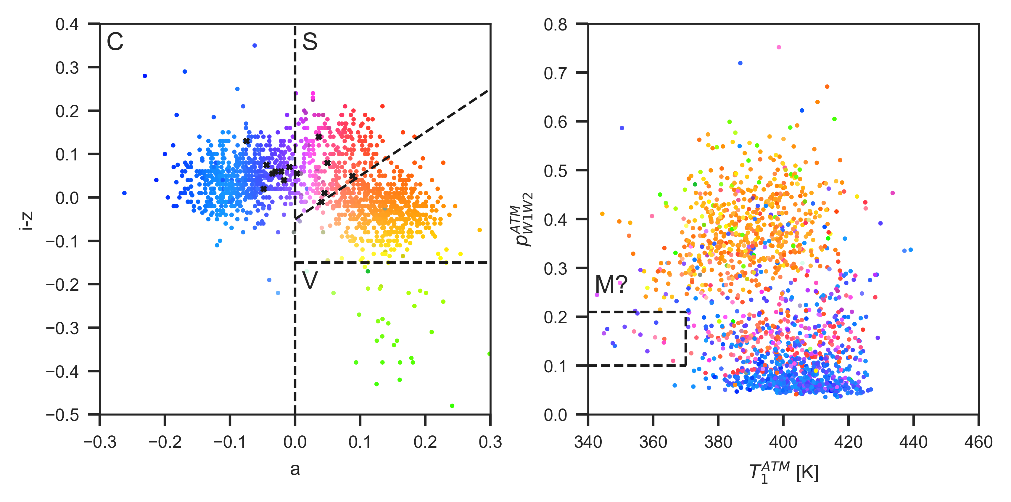
Harris & Drube (2014) argued that the best-fit IR albedo ($p_{IR}$ in the WISE context, $p_{W1W2}$ in the ATM case) and beaming parameter ($\eta$) can be used to select metallic asteroids (M taxonomic type). Their main argument is that objects with high radar albedo values, indicative of metallic objects, display a very narrow distribution of IR albedo ($p_{W1W2}\sim 0.2$), while a larger fraction of objects with unusually high beaming parameter values are seen in the same albedo range. Therefore, objects with large $\eta$ and $p_{W1W2}\sim 0.2$ are good candidates for metallic asteroids. Since WISE data are available for orders of magnitude more objects than radar observations, and metallic objects are interesting in many ways (for discussion see Harris & Drube 2014), it is prudent to critically examine this method.

Due to degeneracy discussed in §2.1.1, ATM fits only for temperature parameter $T_{1}$ and not for $\eta$. The relationship between $T_{1}$ and $\eta$ is given by eq. 4; high $\eta$ corresponds to low $T_{1}$. Therefore, an implication of analysis from Harris & Drube (2014) is that low $T_{1}$ objects with $p_{W1W2}\sim 0.2$ are good candidates for metallic asteroids. We now examine whether IR data discussed here suggest that such outliers exist, and if so, whether they have distinct optical colors.

The right panel in Figure 17 shows that the SDSS-WISE sample does contain objects at the low end of $T_{1}$ range that have $p_{W1W2}\sim 0.2$. By requiring $340<T_{1}/K<370$ and $0.1<p_{W1W2}<0.21$, we select 14 objects out of 1,644 objects in the SDSS-WISE sample (there are 32 selected objects out of 2,479 objects in the high-quality WISE sample), or about 1% of the sample. These candidates for metallic asteroids are listed in Table 4.

Table 4: Candidates for M type (metallic) asteroids^a.

Designation	$g-r$	$r-i$	$logD$	$\sigma_{logD}$	$logT_{1}$	$\sigma_{logT}$	$p_{W1W2}$	$\sigma_{p}$
(497)	0.48	0.15	4.717	0.024	2.542	0.009	0.141	0.015
(844)	0.50	0.19	4.715	0.029	2.541	0.011	0.146	0.019
(1349)	0.51	0.16	4.466	0.040	2.539	0.015	0.175	0.033
(1546)	0.52	0.19	4.468	0.029	2.546	0.011	0.180	0.022
(1670)	0.62	0.14	4.365	0.016	2.549	0.006	0.170	0.012
(1730)	0.58	0.13	4.213	0.025	2.538	0.010	0.166	0.018
(1732)	0.63	0.21	4.397	0.028	2.560	0.011	0.155	0.019
(1860)	0.52	0.20	4.270	0.012	2.554	0.004	0.130	0.009
(1977)	0.56	0.15	4.284	0.021	2.552	0.008	0.164	0.016
(2294)	0.61	0.15	4.206	0.017	2.557	0.006	0.158	0.014
(2407)	0.52	0.17	4.417	0.021	2.550	0.008	0.207	0.019
(2573)	0.61	0.17	4.325	0.020	2.564	0.007	0.110	0.011
(2904)	0.49	0.19	4.209	0.017	2.557	0.006	0.188	0.015
(4813)	0.56	0.24	4.256	0.027	2.560	0.011	0.147	0.018

As the two-dimensional color scheme in Figure 17 illustrates, the IR-selected objects have significantly different optical $a$ color distribution than the full sample: the $a$ color mean and standard deviation for selected objects are $-0.02$ and 0.027, respectively (see the left panel in Figure 17). This difference demonstrates that these objects are not random outliers in the $p_{W1W2}$ vs. $T_{1}$ diagram and provides support to the hypothesis about metallic asteroids advanced by Harris & Drube (2014). Yet, the optical colors of these metallic candidates are not sufficiently unique for an efficient selection using only optical data – for example, a restrictive selection based on $a$ and $i-z$ colors that selects only 8 out of 14 WISE-selected candidates (a selection completeness of $\sim$50%) still results in only 10% sample selection purity (that is, there are about 10 times as many other objects in the SDSS subsample selected by the cut).

Infrared data are required to efficiently select candidates for metallic asteroids. As the right panel in Figure 17 shows, $T_{1}$ selection is more restrictive than $p_{W1W2}$ selection. Therefore, in the context of selecting metallic candidates with a hypothetical two-band survey, having W3 and W4 data would be more useful than W2 and W3 data. On the other hand, for studies requiring $p_{W1W2}$, W1 or W2 band would be a more useful addition to W3 band than the addition of W4 band.

Figure 17: The colored symbols in the left panel show the $a$ vs. $i-z$ SDSS color-color diagram for the same objects as in Figure 16. The symbols’ color code is two-dimensional, according to $a$ and $i-z$ colors (for algorithmic details see Ivezić et al. 2002). The same color coding is used in the right panel to visualize the correlation of optical colors and WISE-based best-fit values of IR albedo ($p_{W1W2}$) and temperature parameter $T_{1}$. It is easy to discern that, for example, objects with $i-z<-0.15$ have high IR albedo, while objects with $a<0$ have predominantly low IR albedo. The dashed lines in the right panel outline selection of 14 candidates for metallic asteroids. Their distribution of optical colors is different from the color distribution for the full sample, as further visualized by showing them as crosses in the left panel. The dashed lines in the left panel outline the distribution of main taxonomic classes, as marked in the panel (C, S and V). This figure was generated using notebooks/analysis/analysis_SDSS.ipynb.

6 Discussion and conclusions

Motivated by a desire to enable transparency and reproducibility of results, and to foster collaborative software development, we release ATM, a general tool for interpreting infrared flux measurements of asteroids. With adequate infrared data, this tool can be used to estimate asteroid sizes, constrain asteroid emissivities at infrared wavelengths, and when optical data are available, also estimate visual albedos. The package also includes data files and example Jupyter Notebooks that can help significantly reduce the time to reproduce published results. All the analysis presented here, including all the figures, tables, and catalogs, can be easily reproduced with these Notebooks.

We emphasize that our analysis presented here, and corresponding catalogs with best-fit sizes and other parameters, are far from definitive and can be improved in various ways. For example, an analysis of emissivity in W1 and W2 bands using Hierarchical Bayesian modeling, similar to our analysis of emissivity in W3 and W4 bands (which could also be improved by optimizing the adopted $\epsilon_{W4}/\epsilon_{W3}$ ratio), would likely further decrease systematic uncertainties. As another example, modern machine learning methods could be used to improve our simplistic algorithm for assigning visual albedo using optical colors (eq. 17). We leave these improvements for future studies by us and the community.

Nevertheless, our results presented here already yield a number of useful conclusions. We show that ATM can match the best-fit size estimates for best-observed objects published in 2016 by the NEOWISE team with a sub-percent bias and a scatter of only 6%. Plausible reasons for this scatter include different outlier rejection algorithms, different treatments of Kirchhoff’s law, and ATM accounting for intrinsic variability, although we cannot exclude other causes. Whatever the reason, the discrepancies are encouragingly small.

Our analysis of various sources of random and systematic size uncertainties show that for the majority of over 100,000 objects with WISE-based size estimates random uncertainties (precision) are about 10% (using W3-based estimates calibrated using high-quality 4-band subsample, see §4.4), and systematic uncertainties within the adopted model framework, such as NEATM, are in the range 10-20%. We estimate that the accuracy of WISE-based asteroid size estimates is in the range 15-20% for most objects, except for unknown errors due to an inadequate modeling framework (such as spherical asteroid approximation). Of course, there is no implied guarantee of Gaussianity and these statements need to be interpreted with care. This result is consistent with the statement that accuracy is about 15% by Mainzer et al. (2016), but somewhat larger than the claim of “errors better than 10%” in Masiero et al. (2011).

The treatment of priors for emissivity $\epsilon(\lambda)$ has a direct and fundamental impact on biases in best-fit size estimates. We note that given this role of $\epsilon(\lambda)$, which is presumably shared by all members of an asteroid family, resulting systematic errors will be shared by all family members and thus cannot be seen when analyzing the per-family scatter in WISE-based optical albedo (Masiero et al., 2018b). Studies of such scatter are insensitive to systematic errors due to incorrect $\epsilon(\lambda)$ and thus cannot be used to constrain the absolute uncertainty, or accuracy, of flux-based size estimates. Only direct size measurements can enable a full understanding of the accuracy of size estimates based on thermal models.

Our ATM results faithfully recover the tri-modal distribution of $\epsilon_{W1W2}$ emissivity related to taxonomic classes discovered by Masiero et al. (2014). Correlations of SDSS colors and WISE-based best-fit model parameters indicate the robustness of the latter, and also give support to the claim that candidate metallic asteroids can be selected using best-fit temperature parameter and IR albedo (Harris & Drube, 2014). However, it should be noted that the condition on priors $\epsilon_{W1}=\epsilon_{W2}=\epsilon_{W1W2}$, introduced because WISE data do not strongly constrain $\epsilon_{W2}$, may not be optimal. For example, we did not investigate ansatz $\epsilon_{W2}=k\,\epsilon_{W1}$, with $k$ different from unity, as we did for $\epsilon_{W3}$ and $\epsilon_{W4}$. We noticed some evidence for $k<1$ when both $\epsilon_{W1}$ and $\epsilon_{W2}$ are free fitting parameters (see §3 and Table 1). Investigation of the optimal value of $k$ using the full high-quality sample and Hierarchical Bayes methodology (as we did for the $\epsilon_{W4}/\epsilon_{W3}$ ratio, see §4.3) may shed new light on the behavior of infrared emissivity/albedo (especially if attempted for taxonomic subsamples defined by optical colors).

We utilized a correlation between SDSS optical colors and optical albedo derived using WISE-based size estimates and developed a method to estimate asteroid sizes with optical data alone, with an uncertainty of about 21% relative to WISE-based size estimates. When systematic errors are included, this small difference in accuracy between IR-based and optical size estimates is further diminished. This remarkable result bodes well for future optical asteroid surveys, such as the Large Synoptic Survey Telescope (Ivezić et al., 2019), which might deliver such size estimates for over 5 million asteroids (Jones et al., 2018, and references therein).

Nevertheless, we point out that adequate infrared data are crucial for breaking the degeneracy between emissivity and asteroid size. An infrared survey with appropriately placed (at least) three bandpasses, and sensitivity to match the LSST sample, could provide a major breakthrough in our knowledge of the emissivity distribution for asteroid population. We also note that laboratory measurements of emissivity can greatly contribute to this endeavor by providing more robust priors for $\epsilon(\lambda)$. Last but not least, direct asteroid size measurements are of paramount importance for validating thermal asteroid models and quantitatively estimating their intrinsic biases, and they should be greatly encouraged and supported.

Appendix A A correction to the quadrature formula for the W3 band

Wright (2013) has derived simple quadrature formulae that can be used to compute in-band fluxes for the four WISE bands from model flux $F_{\nu}^{ast}(\lambda)$. It appears that the provided coefficients for the W3 band can be improved (N. Myhrvold, in prep.). The corrected coefficients are available in ATM package, in method bandpassLambda that can be found in file atm/obs/wise.py. We validated new coefficients by comparing the approximate integral obtained using the quadrature formula to exactly integrated flux for a $T=100$ K black body. The new coefficients match the exact integral to better than 0.2%, while the original coefficients result in a 35% smaller flux. We have verified that the original coefficients for other three bands match exact integrals to sub-percent accuracy.

References

- Astropy Collaboration et al. (2013) Astropy Collaboration, Robitaille, T. P., Tollerud, E. J., et al. 2013, A&A, 558, A33, doi: 10.1051/0004-6361/201322068
- Astropy Collaboration et al. (2018) Astropy Collaboration, Price-Whelan, A. M., Sipőcz, B. M., et al. 2018, AJ, 156, 123, doi: 10.3847/1538-3881/aabc4f
- Bowell et al. (1989) Bowell, E., Hapke, B., Domingue, D., et al. 1989, in Asteroids II, ed. R. P. Binzel, T. Gehrels, & M. S. Matthews, 524–556
- Foreman-Mackey (2016) Foreman-Mackey, D. 2016, The Journal of Open Source Software, 24, doi: 10.21105/joss.00024
- Granvik et al. (2015) Granvik, M., Virtanen, J., Oszkiewicz, D., & Muinonen, K. 2015, OpenOrb: Open-source asteroid orbit computation software, Astrophysics Source Code Library. http://ascl.net/1502.002
- Harris (1998) Harris, A. W. 1998, Icarus, 131, 291, doi: 10.1006/icar.1997.5865
- Harris et al. (1998) Harris, A. W., Davies, J. K., & Green, S. F. 1998, Icarus, 135, 441, doi: 10.1006/icar.1998.6002
- Harris & Drube (2014) Harris, A. W., & Drube, L. 2014, ApJ, 785, L4, doi: 10.1088/2041-8205/785/1/L4
- Hunter (2007) Hunter, J. D. 2007, Computing In Science & Engineering, 9, 90, doi: 10.1109/MCSE.2007.55
- Ivezić et al. (2014) Ivezić, Ž., Connolly, A. J., VanderPlas, J. T., & Gray, A. 2014, Statistics, Data Mining, and Machine Learning in Astronomy: a practical Python guide for the analysis of survey data, Princeton Series in Modern Observational Astronomy (Princeton, NJ: Princeton University Press)
- Ivezić et al. (2001) Ivezić, Ž., Tabachnik, S., Rafikov, R., et al. 2001, AJ, 122, 2749, doi: 10.1086/323452
- Ivezić et al. (2002) Ivezić, Ž., Lupton, R. H., Jurić, M., et al. 2002, AJ, 124, 2943, doi: 10.1086/344077
- Ivezić et al. (2019) Ivezić, Ž., Kahn, S. M., Tyson, J. A., et al. 2019, ApJ, 873, 111, doi: 10.3847/1538-4357/ab042c
- Jones et al. (2001–) Jones, E., Oliphant, T., Peterson, P., et al. 2001–, SciPy: Open source scientific tools for Python. http://www.scipy.org/
- Jones et al. (2018) Jones, R. L., Slater, C. T., Moeyens, J., et al. 2018, Icarus, 303, 181, doi: 10.1016/j.icarus.2017.11.033
- Jurić et al. (2002) Jurić, M., Ivezić, Ž., Lupton, R. H., et al. 2002, AJ, 124, 1776, doi: 10.1086/341950
- Lebofsky & Rieke (1979) Lebofsky, L. A., & Rieke, G. H. 1979, Icarus, 40, 297, doi: 10.1016/0019-1035(79)90074-5
- Mainzer et al. (2015) Mainzer, A., Usui, F., & Trilling, D. E. 2015, Space-Based Thermal Infrared Studies of Asteroids, ed. P. Michel, F. E. DeMeo, & W. F. Bottke, 89–106
- Mainzer et al. (2011) Mainzer, A., Bauer, J., Grav, T., et al. 2011, ApJ, 731, 53, doi: 10.1088/0004-637X/731/1/53
- Mainzer et al. (2012) Mainzer, A., Masiero, J., Grav, T., et al. 2012, ApJ, 745, 7, doi: 10.1088/0004-637X/745/1/7
- Mainzer et al. (2016) Mainzer, A. K., Bauer, J. M., Cutri, R. M., et al. 2016, NASA Planetary Data System, 247, EAR
- Masiero et al. (2014) Masiero, J. R., Grav, T., Mainzer, A. K., et al. 2014, ApJ, 791, 121, doi: 10.1088/0004-637X/791/2/121
- Masiero et al. (2018a) Masiero, J. R., Mainzer, A. K., & Wright, E. L. 2018a, AJ, 156, 62, doi: 10.3847/1538-3881/aacbd4
- Masiero et al. (2018b) —. 2018b, AJ, 156, 62, doi: 10.3847/1538-3881/aacbd4
- Masiero et al. (2011) Masiero, J. R., Mainzer, A. K., Grav, T., et al. 2011, ApJ, 741, 68, doi: 10.1088/0004-637X/741/2/68
- Masiero et al. (2018c) Masiero, J. R., Redwing, E., Mainzer, A. K., et al. 2018c, AJ, 156, 60, doi: 10.3847/1538-3881/aacce4
- McKinney (2010) McKinney, W. 2010, in Proceedings of the 9th Python in Science Conference, ed. S. van der Walt & J. Millman, 51 – 56
- Mommert et al. (2018) Mommert, M., Jedicke, R., & Trilling, D. E. 2018, AJ, 155, 74, doi: 10.3847/1538-3881/aaa23b
- Myhrvold (2018a) Myhrvold, N. 2018a, Icarus, 303, 91, doi: 10.1016/j.icarus.2017.12.024
- Myhrvold (2018b) —. 2018b, Icarus, 314, 64, doi: 10.1016/j.icarus.2018.05.004
- Oliphant (2006) Oliphant, T. E. 2006, A guide to NumPy, Vol. 1
- Parker et al. (2008) Parker, A., Ivezić, Ž., Jurić, M., et al. 2008, Icarus, 198, 138, doi: 10.1016/j.icarus.2008.07.002
- Salvatier et al. (2016) Salvatier, J., Wiecki, T. V., & Fonnesbeck, C. 2016, PeerJ Computer Science, 2, e55, doi: 10.7717/peerj-cs.55
- VanderPlas et al. (2012) VanderPlas, J., Connolly, A. J., Ivezić, Ž., & Gray, A. 2012, in Proceedings of Conference on Intelligent Data Understanding (CIDU), pp. 47-54, 2012., 47–54
- Waskom et al. (2018) Waskom, M., Botvinnik, O., O’Kane, D., et al. 2018, mwaskom/seaborn: v0.9.0 (July 2018), doi: 10.5281/zenodo.1313201. https://doi.org/10.5281/zenodo.1313201
- Wright et al. (2018) Wright, E., Mainzer, A., Masiero, J., et al. 2018, ArXiv e-prints. https://arxiv.org/abs/1811.01454
- Wright (2007) Wright, E. L. 2007, ArXiv Astrophysics e-prints
- Wright (2013) Wright, E. L. 2013, in American Astronomical Society Meeting Abstracts, Vol. 221, American Astronomical Society Meeting Abstracts #221, 439.05
- Wright et al. (2010) Wright, E. L., Eisenhardt, P. R. M., Mainzer, A. K., et al. 2010, AJ, 140, 1868, doi: 10.1088/0004-6256/140/6/1868