Decision Making with Machine Learning and ROC Curves

Abstract. The Receiver Operating Characteristic (ROC) curve is a representation of the statistical information discovered in binary classification problems and is a key concept in machine learning and data science. This paper studies the statistical properties of ROC curves and its implication on model selection. We analyze the implications of different models of incentive heterogeneity and information asymmetry on the relation between human decisions and the ROC curves. Our theoretical discussion is illustrated in the context of a large data set of pregnancy outcomes and doctor diagnosis from the Pre-Pregnancy Checkups of reproductive age couples in Henan Province provided by the Chinese Ministry of Health.

Keywords: ROC Curve, Binary Classification, Neyman Pearson Lemma, Incentive Heterogeneity, Information Asymmetry.

1 Introduction

In the era of artificial intelligence, much attention has been drawn to the potential of machine learning in assisting human decision making. Among the recent headlines, Google used a deep learning algorithm to detect diabetic retinopathy in retinal fundus photographs (Gulshan et al. (2016)). Long et al. (2017) proposes a new deep learning algorithm, CC-Cruiser, which can be used to diagnose cataracts and provide treatment advice. In the economics literature, Currie and MacLeod (2017)’s analysis of the decision making of physicians suggests the possibility of improvements that can both benefit patients and reduce medical expenses.

In this paper, we focus on the binary classification decision making problem, i.e. a choice between “yes” and “no”, or $1$ and $0$. Binary classification is a foundational building block of statistical decision making in a variety of disciplines including machine learning, data science, and econometrics. It takes different forms and interpretations in different empirical settings: “ill or healthy” in a medical diagnosis by physicians, “jail or release” in a verdict by sitting Judges, and “accept or reject” by a collage admission committee.

A key concept that is used to evaluate the quality of binary classification and prediction is the Receiver Operating Characteristic (ROC) Curve, which essentially measures the diagnostic performance of a binary classifier as its cutoff threshold is varied. Since its first appearance in Fisher (1936), ROC curves and its variants are widely used in analyzing empirical data. However, its statistical properties do not appear to be well-understood. This paper serves to bridge such an important gap, and present statistical properties of ROC curves in the context of decision making under incentive heteroscedasticity and information asymmetry.

For a data set with labels $Y_{i}\in\{0,1\}$, and features $X_{i},i=1,\ldots,n$, a learning algorithm makes predictions $\hat{Y}_{i}\in\{0,1\}$ for $Y_{i}$. An algorithm that generates a higher proportion of correct predictions, defined as the accuracy

$$\text{ACC}=\frac{1}{n}\sum_{i=1}^{n}\mathds{1}\left(\hat{Y}_{i}=Y_{i}\right),$$

naturally has more appeal.

However, accuracy itself is unlikely to be sufficient to characterize the quality of prediction algorithms. In the National Free Pre-Pregnancy Check-ups (NFPC) data set that we studied as an application of this paper, the accuracy of doctors’ diagnosis of high-risk pregnancy $\hat{Y}_{i}$ in predicting birth defects ($Y_{i}$) is about 80%. Yet less than 5% of the births are abnormal. A simple prediction of all pregnancy as low risk would result in an accuracy of 95%. Nevertheless, the precision of doctor’s diagnosis among the abnormal births, or the true positive rate (TPR), is much higher than the naive prediction of all normal births (where the TPR is by definition zero). For this reason, the pair of TPR and false positive rate (FPR) are to be considered in tandem in evaluating a given set of predictions:

$$\text{TPR}=\sum_{i=1}^{n}Y_{i}\hat{Y}_{i}/\sum_{i=1}^{n}Y_{i},\quad\text{FPR}=\sum_{i=1}^{n}\left(1-Y_{i}\right)\hat{Y}_{i}/\sum_{i=1}^{n}\left(1-Y_{i}\right).$$

In a statistical setting, a prediction method (based on either machine learning or a binary choice econometric model) typically generates a function of features that represents a sample estimate of the probability of the label taking value $1$ conditional on the features: $\hat{p}\left(X_{i}\right)\in\left[0,1\right]$. The sample ROC is a transformation of the estimated probability function $\hat{p}\left(X_{i}\right)$. It is the collection of the set of all TPR/FPR pairs corresponding to decision rules of the form of $\hat{Y}_{i}=\mathds{1}\left(\hat{p}\left(X_{i}\right)>c\right)$ when $c$ varies from $0$ to $1$. Essentially, ROC curves present the tradeoff between TPR and FPR for different cutoff thresholds. Figure 1 shows the typical shape of a ROC curve (the blue line), e.g. resembling those reported in numerous science papers. The red dot represents the aggregate TPR/FPR of human decision makers (such as doctors diagnosing diseases) in the observed data that is typically benchmarked by the ROC curves generated by machine learning algorithms.

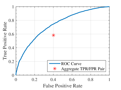
Figure 1: A typical ROC curve

Note that papers such as Kleinberg et al. (2018) and Elliott and Lieli (2013) use loss (cost) function to specify the tradeoff between under-detection and over-detection rates, which is closely related to the ROC curve.

The focal point of our paper is to study the fundamental properties of ROC curves and proposes a statistical inference to the ROC curve. From Bamber (1975), many papers such as Fawcett (2006) and Hand and Till (2001)) study using the area under curve (AUC), a number instead of a curve, to measure the overall performance of a binary classifier. In this paper, we also present the inference of AUC and its implication for model selection.

Benchmarking the performance of machine algorithm, normally presented by a ROC curve, with that of a human decision maker, presented by a pair of false positive and true positive rates, is a common practice. For example, Rajpurkar et al. (2017) trained a 34-layer convolutional neural network to process ECG sequences and compared its performance to 6 cardiologists. Esteva et al. (2017) proposed a deep convolutional neural network structure for skin cancer classification and claimed that the model outperforms the average dermatologist. Kermany et al. (2018) proposed an image-based deep learning model to classify macular degeneration and concluded that it outperforms human. The conclusions of these papers are mostly based on observing an empirical pair of true positive and false positive rates that lie strictly below the ROC curve formed by the machine classification algorithm, implying that machines can achieve a higher TPR for a given FPR, or a lower FPR for a given TPR. However, an important message of our current paper is to caution against such interpretations without a deeper understanding of the human decision making process: such findings can be rationalized not only by the superior information quality of machine learning algorithms, but also by the incentive heterogeneity of human decision makers who can be as intelligent as machine learning algorithms in processing statistical information from observational data.

To illustrate an issue of concern, consider Figure 2, in which a collection of human decision makers, denoted $j=1,\ldots,J$, all lie approximately on the machine-learned ROC. This is the case if they employed decision rules $\hat{Y}_{i}=\mathds{1}\left(\hat{p}\left(X_{i}\right)>c_{i}\right)$ with the same $\hat{p}\left(\cdot\right)$ function but with different individual cutoff points $c_{i}$. Yet, after aggregating over all decision makers, the aggregate TPR/FPR pair lies visibly below the ROC.

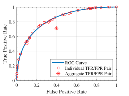
Figure 2: Individual and Aggregate TPR/FPR Pairs: Perspective of Jensen’s Inequality

This is an immediate artifact of Jensen’s inequality due to the concavity of the observed ROC, and bears no implication on the comparison between the qualities of the machine learning algorithm and human decision makers. An optimal ROC is necessarily concave (Lemma A.1). This simple observation appears to have gone largely unnoticed by the literature.

More precisely, as long as the collection of humans’ individual TPR/FPR points can be represented by a concave curve, the aggregated humans’ TPR/FPR must fall below the curve of humans’ individual TPR/FPR points. Let $\alpha_{j}$ denote FPR and $\beta_{j}$ denote TPR, and suppose they are related by $\beta=f\left(\alpha\right)$, where $f\left(\cdot\right)$ is concave. Then by Jensen’s inequality:

$$\bar{\beta}=\frac{1}{J}\sum_{j=1}^{J}\beta_{j}=\frac{1}{J}\sum_{j=1}^{n}f\left(\alpha_{j}\right)<f\left(\frac{1}{J}\sum_{j=1}^{J}\alpha_{i}\right)=f\left(\bar{\alpha}\right).$$

Furthermore, when incentive heterogeneity is present, a decision maker may also set her cutoff value $c$ based on observed features $X$, denoted as $c\left(X_{i}\right)$. As shown in subsection 5.2.1, in this case, the TPR/FPR pair of a single decision maker is also below the optimal ROC curve. Lemma A.2 presents a formal proof. The foregoing discussion highlights the need to understand and correctly interpret the statistical properties of ROC curves.

To motivate and empirically illustrate our theoretical discussion, we make use of a data set of high-risk pregnancy diagnosis with more than a million observations collected in the NFPC administered by the Chinese Ministry of Health. The checkup is offered free of charge to newly-wed couples who are either expecting or who are planning to conceive. The data set contains more than 300 features, including indicators from medical examinations and clinical tests, individual and family history of diseases and drug usage, pregnancy history, and demographic characteristics, etc. The label is whether the birth outcome is normal or involves defects. Most importantly, the data set also contains the diagnosis by doctors regarding the risk level of each pregnancy.

The rest of this paper are as follows. In section 2, we offer an in-depth analysis of the properties of the ROC in the context of a statistical model and its relationship with loss functions in decision making. Section 3 and 4 develop and study methods for the statistical inference of ROC and for related model estimation and selection issues. These two sections involve technical econometrics results that can be skipped for readers mostly interested in economic insights. Section 5 analyze the issues and caveats when comparing performance between humans and machine algorithms. In section 6, we present a detailed empirical application using the NFPC data set. Section 7 concludes.

2 Neyman Pearson Lemma and Decision Rules

In a standard statistical model, the data set $Y_{i},X_{i},i=1,\ldots,n$ is typically assumed to be drawn i.i.d. (identically and independently distributed) from an underlying population. There is a true probability function $p\left(X_{i}\right)=\mathbb{P}\left(Y_{i}=1|X_{i}\right)$, also known as the propensity score function in the treatment effect literature. We will invoke (uniform) law of large numbers and convergence in probability whenever they may apply under plausible assumptions. For this purpose, for $\mathbb{X}$ the support of $X_{i}$, we assume that $\hat{p}\left(X_{i}\right)$ converges uniformly over $\mathbb{X}$ to a deterministic limit function $q\left(X_{i}\right)$ when $n$ increases without bound:

$$\sup_{x\in\mathbb{X}}\left|\hat{p}\left(x\right)-q\left(x\right)\right|\overset{p}{\longrightarrow}0,\quad\text{as}\quad n\rightarrow\infty.$$

In the above, if the model that is used to estimate $\hat{p}\left(X_{i}\right)$ is correctly specified, $q\left(\cdot\right)=p\left(\cdot\right)$. If a misspecified model is used to obtain $\hat{p}\left(X_{i}\right)$, it is possible that $q\left(\cdot\right)\neq p\left(\cdot\right)$.

2.1 Neyman Pearson Lemma

Binary decision making is inherently related to parametric hypothesis testing. In the terminology of hypothesis testing, $Y=0$ is often denoted as the null hypothesis and $Y=1$ as the alternative hypothesis. The TPR/FPR pair corresponds to the power (one minus Type II error) and the size (Type I error) of a test. For a general classification rule $\hat{Y}_{i}=\mathds{1}\left(X_{i}\in R\right)$, where $R$ is known as the rejection region in hypothesis testing, the law of large numbers implies that the sample TPR/FPR pair corresponding to each $R$ converges to their population analogs, denoted as PTPR and PFPR

$$\begin{split}\text{TPR}&\overset{\mathbb{P}}{\longrightarrow}\text{PTPR}\equiv\frac{\mathbb{E}\left[Y_{i}\mathds{1}\left(X_{i}\in R\right)\right]}{p},\\ \text{FPR}&\overset{\mathbb{P}}{\longrightarrow}\text{PFPR}\equiv\frac{\mathbb{E}\left[\left(1-Y_{i}\right)\mathds{1}\left(X_{i}\in R\right)\right]}{1-p}.\end{split}$$

In the above, $p=\mathbb{E}\left[Y_{i}\right]=\int p\left(x\right)f\left(x\right)\mathrm{d}x$ is the overall population portion of positive labels, where for simplicity we assume that $X$ has a density $f\left(x\right)$, which can be broadly interpreted using generalized functions to include probability mass functions for discrete $X$. By the law of iterated expectation,

$$\begin{split}\text{PTPR}=\frac{1}{p}\int p\left(x\right)\mathds{1}\left(x\in R\right)f\left(x\right)\mathrm{d}x,\quad\text{PFPR}=\frac{1}{1-p}\int\left(1-p\left(x\right)\right)\mathds{1}\left(x\in R\right)f\left(x\right)\mathrm{d}x.\end{split}$$

Recall the Bayes law

$$\begin{split}f\left(X|Y=1\right)=\frac{f\left(X\right)p\left(X\right)}{p},\quad f\left(X|Y=0\right)=\frac{f\left(X\right)\left(1-p\left(X\right)\right)}{1-p}.\end{split}$$

Therefore we can equivalently write

$$\begin{split}\text{PTPR}=\int\mathds{1}\left(X\in R\right)f\left(X|Y=1\right)\mathrm{d}X,\quad\text{PFPR}=\int\mathds{1}\left(X\in R\right)f\left(X|Y=0\right)\mathrm{d}X.\end{split}$$

Consequently, PTPR is the probability of rejection under the alternative hypothesis, namely the power of the test; PFPR is the probability of rejection under the null hypothesis, namely the size of the test. In the population limit, the ROC is therefore a plot of power against size, for the collection of rejection areas determined by $R=\mathds{1}\left(q\left(X_{i}\right)>c\right)$ when $c$ ranges over $\left[0,1\right]$.

The classical Neyman Pearson Lemma states that the collection of likelihood ratio tests

$$\begin{split}R_{NP}\left(d\right)=\biggl{\{}x:\frac{f\left(X|Y=1\right)}{f\left(X|Y=0\right)}>d\biggr{\}},\end{split}$$

where $d\in\left(0,\infty\right)$ varies, are most powerful tests that maximize power for whatever size it achieves. By the Bayes law, write

$$\begin{split}R_{NP}\left(d\right)=\biggl{\{}x:\frac{p\left(x\right)}{1-p\left(x\right)}>d\frac{p}{1-p}\biggr{\}}=\biggl{\{}x:p\left(x\right)>c=\frac{dp}{1-p+dp}\biggr{\}}.\end{split}$$

Consequently, the ROC corresponding to the decision rules

$$\begin{split}\hat{y}=\mathds{1}\left(p\left(x\right)>c\right)\quad\text{for $c$ varying between $0$ and $1$,}\end{split}$$

has the Neyman-Pearson optimality that it lies weakly above the PTPR/PFPR pair of any other decision rule $\hat{y}=\mathds{1}\left(x\in R\right)$ for any given $R$, or equivalently the ROC of any alternative collection of decision rules.

Lemma A.1 in the Appendix shows that the optimal ROC is necessarily a concave function. A non-optimal ROC, on the other hand, need not be concave, and can even lie above the 45 degree line.

2.2 Loss Function in Decision Making

The decision theoretic framework in Elliott and Lieli (2013) and Kleinberg et al. (2018) balances the loss of false positive decision vs. the loss of false negative decision through a cost (loss) function. Since the choice decision depends only on the utility difference and is invariant with respect to the addition of a normalizing constant, without loss of generality we first consider minimizing expected cost based on the following cost matrix, where the cost of correct classifications is normalized to zero:

Table 1: Loss Matrix

	$\hat{Y}=0,\text{Accept}$	$\hat{Y}=1,\text{Reject}$
$Y=0$	$0$	$c_{0R}$
$Y=1$	$c_{1A}$	$0$

The (negative of the) expected loss governed by this cost matrix is then

$$\begin{split}&-\int\left[C_{0R}\mathds{1}\left(x\in R,Y=0\right)+C_{1A}\mathds{1}\left(x\in R^{c},Y=1\right)\right]\mathrm{d}F\left(x,Y\right)\\ =&-\int\biggl{[}\mathds{1}\left(x\in R\right)\left(1-p\right)C_{0R}f\left(x|Y=0\right)+\mathds{1}\left(x\in R^{c}\right)pC_{1A}f\left(x|Y=1\right)\biggr{]}\mathrm{d}x\\ =&-C_{0R}\mathbb{P}\left(X\in R,Y=0\right)+C_{1A}\mathbb{P}\left(X\in R,Y=1\right)+\text{const}\end{split}$$ (1)

where $\text{const}=-C_{1A}\mathbb{P}\left(Y=1\right)$ does not depend on the rejection region $R$. This takes the same form of a linear combination of PTPR and PFPR, i.e. $\phi\mathrm{PTPR}-\eta\mathrm{PFPR}$, where $\phi=pC_{1A}$ and $\eta=\left(1-p\right)C_{0R}$.

$$\begin{split}\phi\text{PTPR}-\eta\text{PFPR}=&\frac{\phi}{p}\mathbb{P}\left(Y=1,X\in R\right)-\frac{\eta}{1-p}\mathbb{P}\left(Y=0,X\in R\right)\\ =&\int\left[\mathds{1}\left(X\in R\right)\frac{\phi}{p}p\left(X\right)-\mathds{1}\left(X\in R\right)\frac{\eta}{1-p}\left(1-p\left(X\right)\right)\right]f\left(X\right)\mathrm{d}X\end{split}$$ (2)

By inspection, the optimal rule $R_{c}$ that maximizes this linear combination is given by

$$\begin{split}R_{c}&=\biggl{\{}X:\frac{\phi}{p}p\left(X\right)>\frac{\eta}{1-p}\left(1-p\left(X\right)\right)\ \biggr{\}}=\biggl{\{}X:p\left(X\right)>c=\frac{\eta/(1-p)}{\phi/p+\eta/(1-p)}\biggr{\}}.\end{split}$$ (3)

Therefore, for each $c$, the implied $R_{c}$ corresponds to the maximizer of $\phi\text{PTPR}-\eta\text{PFPR}$ for some (nonunique) choice of $\phi$ and $\eta$ which in turn determine $c$. Consequently, for this $c$ and the resulting $R_{c}$, it is not possible to choose an alternative $R$ in order to increase PTPR while keeping PFPR unchanged, or to decrease PFPR while keeping PTPR unchanged. In other words, other classification rules that result in at least as much as this PTPR will necessarily have the same or higher PFPR. Equivalently, any other classification rule that results in at most this PFPR will have the same or lower PTPR. Since the choice of $C_{0R}$ and $C_{1A}$ is subjective and lacks consensus, it is common to draw a curve of FPR and TPR according to different combination of $C_{0R}$ and $C_{1A}$ in an ROC curve.

2.3 Additional Remarks

Randomized tests

are sometimes used to obtain a desired size when the observations $X$ have a discrete distribution, and has its analog in binary classification as a randomized classification rule.

However, for size levels that can be achieved by a function of the features, randomization only serves to dilute power. Specifically, a randomized classifier is a decision rule

$$\begin{split}\hat{Y}=\phi\left(X,U\right)\in\{0,1\}\quad\text{were}\quad U\perp Y|X.\end{split}$$

The condition $U\perp Y|X$ rules out information about $Y$ that is not already contained in $X$.

The resulting PFPR and PTPR can now be written as

$$\begin{split}\text{PTPR}=\frac{1}{p}\iint\phi\left(X,U\right)f\left(U|X\right)\mathrm{d}Up\left(X\right)f\left(X\right)\mathrm{d}X\end{split}$$

and

$$\begin{split}\text{PFPR}=\frac{1}{1-p}\iint\phi\left(X,U\right)f\left(U|X\right)\mathrm{d}U\left(1-p\left(X\right)\right)f\left(X\right)\mathrm{d}X\end{split}$$

Given $\phi$ and $\eta$, the maximizing $\phi\left(X,U\right)$ of a linear combination of $\phi\text{PTPR}-\eta\text{PFPR}$ satisfies

$$\begin{split}\int\phi\left(X,U\right)f\left(U|X\right)\mathrm{d}U=\mathds{1}\left(p\left(X\right)>c\right),\end{split}$$

for $c$ determined by $\phi$ and $\eta$ as in (3). A solution is given by (3): $\phi\left(X,U\right)=\mathds{1}\left(p\left(X\right)>c\right)$.

Alternative representations

of the ROC are possible. Consider the following question: conditional on a machine diagnosis of being high risk, what is the probability of actually being high risk. In other words, we would like to calculate, by Bayes law:

$$\begin{split}&\mathbb{P}\left(Y=1|\hat{Y}=1\right)=\frac{\mathbb{P}\left(Y=1,\hat{Y}=1\right)}{\mathbb{P}\left(\hat{Y}=1\right)}\\ =&\frac{p\times\mathbb{P}\left(\hat{Y}=1|Y=1\right)}{p\times\mathbb{P}\left(\hat{Y}=1|Y=1\right)+(1-p)\times\mathbb{P}\left(\hat{Y}=1|Y=0\right)}=\frac{p\times\text{TPR}}{p\times\text{TPR}+(1-p)\times\text{FPR}}\end{split}$$

In the above, $p$ is given by raw data. Next, each point on the ROC curve corresponds to a $\text{TPR}/\text{FPR}$ pair. Therefore, for each point on the ROC curve, we can calculate $\mathbb{P}\left(Y=1|\hat{Y}=1\right)$. Connecting these numbers will produce a “posterior odds” curve.

For example, with perfect classification, $\text{FPR}=0$ and $\text{TPR}=1$, $\mathbb{P}\left(Y=1|\hat{Y}=1\right)=1$. With random guessing, the ROC curve is the 45 degree line, where $\text{FPR}=\text{TPR}$, then $\mathbb{P}\left(Y=1|\hat{Y}=1\right)=\mathbb{P}\left(Y=1\right)$, same as the raw sample unconditional probability.

Sampling Errors

differentiates the ROC for the binary classification problem from classical hypothesis testing problems. In the size versus power tradeoff in classical hypothesis testing, the conditional densities of the features under both the null and the alternative, $f\left(X|Y=0\right)$ and $f\left(X|Y=1\right)$, are known and fully specified. In contrast, in binary classification these quantities, or equivalently the propensity score $p\left(x\right)$, need to be estimated from the training data set and are thus subject to sampling errors.

In the population analysis we abstract away from such sampling errors, a topic that we defer to in the estimation and inference sections. Precise knowledge of the correctly specified population propensity score $p\left(X\right)$ is not feasible in finite samples. If the features $X_{i}$ are supported on a small number of discrete points, $p\left(x\right)$ can be estimated by the sample frequency counts of $Y$ for each value in the support of $\mathbb{X}$:

$$\begin{split}\hat{p}\left(X=k\right)=\frac{\sum_{i=1}^{n}Y_{i}\mathds{1}\left(X_{i}=k\right)}{n_{k}},\quad n_{k}=\sum_{i=1}^{n}\mathds{1}\left(X_{i}=k\right).\end{split}$$

When the features are continuously distributed or take a large number of discrete values, regularization methods such as parametric assumptions, sampling splitting, nonparametric regression, penalization, etc, are needed to reduce overfitting and to obtain $\hat{p}\left(x\right)$ that has out of sample predictive powers.

The $\hat{p}\left(x\right)$ estimated from the training data is likely to be misspecified in the holdout sample, or converge to a $q\left(x\right)$ that is misspecified in the population. In these situations, it may be difficult to find a dominating ROC among several competing models, as their corresponding ROCs are likely to cross each other. Choosing among these ROCs involves a subjective choice of criteria, such as the F-score or the Area Under Curve (AUC). The sense in which these alternative loss functions offer better model selection criteria than the usual measurements (such as mean square error, accuracy, or entropy divergence) remains to be investigated. Huang and Ling (2005) argued both theoretically and empirically for the advantage of using AUC over accuracy.

The duality

between binary classification and classical hypothesis testing also suggests a conditional version of the Neyman-Pearson lemma that uses the conditional density of $x_{1}$ given $x_{2}$: $f\left(x_{1}|x_{2},y=\{1,0\}\right)$ and that employs a critical value $c\left(x_{2}\right)$ that depends on $x_{2}$ only:

$$\begin{split}\tilde{R}=\biggl{\{}x:\frac{f\left(x_{1}|x_{2},y=1\right)}{f\left(x_{1}|x_{2},y=0\right)}>c\left(x_{2}\right)\biggr{\}}\end{split}$$ (4)

where $\tilde{R}$ is the collection of rejection areas. This can be justified by minimizing expected conditional Bayesian loss given $x_{2}$, where the prior and the loss can depend on $x_{2}$ (only):

$$\begin{split}\tilde{R}=&\arg\min_{R}p_{1}\left(x_{2}\right)\ell_{1}\left(x_{2}\right)\int_{x_{1}\in R}f\left(x_{1}|x_{2},y=0\right)\mathrm{d}x_{1}\\ &\hskip 7.22743pt+\left(1-p_{1}\left(x_{2}\right)\right)\ell_{0}\left(x_{2}\right)\int_{x_{1}\in R^{c}}f\left(x_{1}|x_{2},y=1\right)\mathrm{d}x_{1}.\end{split}$$

In the above, $\ell_{0}\left(x_{2}\right)$ is the loss of rejecting when the null is true, and $\ell_{1}\left(x_{2}\right)$ is the loss of not rejecting when the null is false. $p_{1}\left(x_{2}\right)$ is the conditional prior probability of the null, and $\left(1-p_{1}\left(x_{2}\right)\right)$ is the conditional prior probability of the alternative.

While the rejection region now also takes a form of (4), the determination of $c\left(x_{2}\right)$ also involves knowledge of $\frac{f\left(x_{2}|y=1\right)}{f\left(x_{2}|y=0\right)}$ in addition to the prior probabilities and loss function matrix.

3 Statistical Inference of ROC Curves

In this section we derive asymptotic pointwise confidence bands for an estimated ROC to account for its sampling uncertainty. Confidence bands can be useful for testing the statistical performance of a ROC curve or testing whether one ROC lies above another. These results are technical in nature and are valid under conventional regularity conditions. For brevity and clarify we present the main results. Detailed verification steps are available from the authors upon request. In reference of Figure 1, confidence bands can be constructed vertically or horizontally. We begin with the vertical construction, and then show that it is also valid in a horizontal sense.

3.1 Vertical Construction of Confidence Bands

For tractability, we consider parametric models of $p\left(X_{i},\theta\right)$ under i.i.d sampling assumptions. A consistent estimate of $\hat{\theta}$ can be obtained by maximum likelihood or other methods, such that $\hat{\theta}\overset{p}{\longrightarrow}\theta_{0}$, with an asymptotic linear influence function representation:

$$\begin{split}\sqrt{n}\left(\hat{\theta}-\theta_{0}\right)=\frac{1}{\sqrt{n}}\sum_{i=1}^{n}\kappa_{i}+o_{P}\left(1\right),\quad\text{where}\quad\kappa_{i}=\kappa\left(y_{i},x_{i}\right)\end{split}$$ (5)

In the sample, the power and size corresponding to the classification rule based on $p\left(X_{i},\theta\right)$ and a threshold value of $c$ are given by

$$\begin{split}\hat{\beta}\left(c\right)=\frac{1/n\sum_{i=1}^{n}y_{i}\mathds{1}\left(p\left(x_{i},\hat{\theta}\right)>c\right)}{\hat{p}},\quad\hat{\alpha}\left(c\right)=\frac{1/n\sum_{i=1}^{n}\left(1-y_{i}\right)\mathds{1}\left(p\left(x_{i},\hat{\theta}\right)>c\right)}{1-\hat{p}}\end{split}$$

To simplify notation let $\hat{c}_{\alpha}=\hat{\alpha}^{-1}\left(\alpha\right)$ and $\hat{\beta}_{\alpha}=\hat{\beta}\left(\hat{c}_{\alpha}\right)=\hat{\beta}\left(\hat{\alpha}^{-1}\left(\alpha\right)\right)$. Non-continuity can be handled by redefinining $\hat{c}_{\alpha}=\inf\{c:\hat{\alpha}\left(c\right)>\alpha\}$. The population analogs of the power and size curves are defined by

$$\begin{split}\beta\left(c\right)=\frac{1}{p}\mathbb{E}\left[p\left(X\right)\mathds{1}\left(p\left(X,\theta_{0}\right)>c\right)\right],\quad\alpha\left(c\right)=\frac{1}{1-p}\mathbb{E}\left[\left(1-p\left(X\right)\right)\mathds{1}\left(p\left(X,\theta_{0}\right)>c\right)\right].\end{split}$$

Similarly let $c_{\alpha}=\alpha^{-1}\left(\alpha\right)$ and $\beta_{\alpha}\equiv\beta\left(\alpha\right)=\beta\left(c_{\alpha}\right)=\beta\left(\alpha^{-1}\left(\alpha\right)\right)$.

The goal is to construct an asymptotic confidence inteval for $\beta_{\alpha}$ based on $\hat{\beta}_{\alpha}$ for each $\alpha$, in the form of $\left(\hat{\beta}_{\alpha}-\hat{d},\hat{\beta}_{\alpha}+\hat{d}\right)$, to ensure a given approximate coverage probability

$$\begin{split}\lim\inf_{n\rightarrow\infty}\mathbb{P}\left(\hat{\beta}_{\alpha}-\hat{d}\leq\beta_{\alpha}\leq\hat{\beta}_{\alpha}+\hat{d}\right)\geq 1-\eta.\end{split}$$ (6)

Typical choices of $\eta$ are $1\%,5\%$ and $10\%$. This is achieved by deriving the asymptotic distribution of $\hat{\beta}_{\alpha}-\beta_{\alpha}$, which in turn can be based on an influential function representation in the form of

$$\begin{split}\sqrt{n}\left(\hat{\beta}_{\alpha}-\beta_{\alpha}\right)=\frac{1}{\sqrt{n}}\sum_{i=1}^{n}\psi_{i}+o_{\mathbb{P}}\left(1\right),\quad\text{where}\quad\psi_{i}=\psi\left(y_{i},x_{i},\alpha\right).\end{split}$$ (7)

It follows from (7) that

$$\begin{split}\sqrt{n}\left(\hat{\beta}_{\alpha}-\beta_{\alpha}\right)\overset{d}{\longrightarrow}N\left(0,\sigma^{2}\right),\quad\text{where}\quad\sigma^{2}=Var\left(\psi_{i}\right).\end{split}$$

For a consistent estimate $\hat{\sigma}^{2}\overset{\mathbb{P}}{\rightarrow}\sigma^{2}$, we can form $\hat{d}=\frac{1}{\sqrt{n}}\hat{\sigma}\Phi^{-1}\left(1-\eta/2\right)$. In the following we present the procedure to derive (7) and to obtain $\hat{\sigma}^{2}$. Verifying (7) is also important for validating the use of resampling methods such as the bootstrap for confidence interval construction.

To show (7) we begin with defining the sample moment conditions,

$$\begin{split}Q_{n}\left(\theta,c,\beta\right)=&\frac{1}{n}\sum_{i=1}^{n}y_{i}\left(\mathds{1}\left(p\left(x_{i},\theta\right)>c\right)-\beta\right),\\ P_{n}\left(\theta,c,\alpha\right)=&\frac{1}{n}\sum_{i=1}^{n}\left(1-y_{i}\right)\left(\mathds{1}\left(p\left(x_{i},\theta\right)>c\right)-\alpha\right).\end{split}$$

and their the population analogs

$$\begin{split}Q\left(\theta,c,\beta\right)=&\mathbb{E}\left[p\left(X\right)\left(\mathds{1}\left(p\left(X,\theta\right)>c\right)-\beta\right)\right],\quad\\ P\left(\theta,c,\alpha\right)=&\mathbb{E}\left[\left(1-p\left(X\right)\right)\left(\mathds{1}\left(p\left(X,\theta\right)>c\right)-\alpha\right)\right].\end{split}$$

For a correctly specified model, $p\left(X\right)=p\left(X,\theta_{0}\right)$. By construction

$$\begin{split}Q_{n}\left(\hat{\theta},\hat{c}_{\alpha},\hat{\beta}_{\alpha}\right)=o_{\mathbb{P}}\left(\frac{1}{n}\right),\quad P_{n}\left(\hat{\theta},\hat{c}_{\alpha},\alpha\right)=o_{\mathbb{P}}\left(\frac{1}{n}\right),\quad Q\left(\theta_{0},c_{\alpha},\beta_{\alpha}\right)=0,\quad P\left(\theta_{0},c_{\alpha},\alpha\right)=0.\end{split}$$

To account for the discontinuity of the sample moment conditions as a function of the parameters, we assume that the parametric propensity score $p\left(X_{i},\theta\right)$ satisfies a typical stochastic equicontinuity condition (Chapters 36 and 37 of Newey and McFadden (1994)):

$$\begin{split}P_{n}\left(\hat{\theta},\hat{c}_{\alpha},\alpha\right)-P_{n}\left(\theta_{0},c_{\alpha},\alpha\right)-P\left(\hat{\theta},\hat{c}_{\alpha},\alpha\right)+P\left(\theta_{0},c_{\alpha},\alpha\right)=o_{\mathbb{P}}\left(\frac{1}{\sqrt{n}}\right).\end{split}$$

The first term is $o_{\mathbb{P}}\left(\frac{1}{n}\right)$. Therefore

$$\begin{split}P_{n}\left(\theta_{0},c_{\alpha},\alpha\right)+P\left(\hat{\theta},\hat{c}_{\alpha},\alpha\right)-P\left(\theta_{0},c_{\alpha},\alpha\right)=o_{\mathbb{P}}\left(\frac{1}{\sqrt{n}}\right).\end{split}$$

Then by first order Taylor expansion,

$$\begin{split}\sqrt{n}\left(\hat{c}_{\alpha}-c_{\alpha}\right)=-\left(\frac{\partial P\left(\theta_{0},c_{\alpha},\alpha\right)}{\partial c}\right)^{-1}\left[\sqrt{n}P_{n}\left(\theta_{0},c_{\alpha},\alpha\right)+\frac{\partial P\left(\theta_{0},c_{\alpha},\alpha\right)}{\partial\theta}\sqrt{n}\left(\hat{\theta}-\theta_{0}\right)\right]+o_{\mathbb{P}}\left(1\right),\end{split}$$

Under correct model specification, for $f_{p}\left(\cdot\right)$ the implied density of $p\left(X\right)$ induced by $X$,

$$\begin{split}P_{c}\left(\theta_{0},c_{\alpha},\alpha\right)\equiv\frac{\partial P\left(\theta_{0},c_{\alpha},\alpha\right)}{\partial c}=-\left(1-c_{\alpha}\right)f_{p}\left(c_{\alpha}\right).\end{split}$$

Without a specific function form for $p\left(X,\theta\right)$ we cannot provide a further analytic expression for $P_{\theta}\left(\theta_{0},c_{\alpha},\alpha\right)=\frac{\partial P\left(\theta_{0},c_{\alpha},\alpha\right)}{\partial\theta}$, but it can be estimated consistently using finite sample numerical derivatives.

To derive (7) we continue to make use of stochastic equicontinuity

$$\begin{split}Q_{n}\left(\hat{\theta},\hat{c}_{\alpha},\hat{\beta}_{\alpha}\right)-Q_{n}\left(\theta_{0},c_{\alpha},\beta_{\alpha}\right)-Q\left(\hat{\theta},\hat{c}_{\alpha},\hat{\beta}_{\alpha}\right)+Q\left(\theta_{0},c_{\alpha},\beta_{\alpha}\right)=o_{\mathbb{P}}\left(\frac{1}{\sqrt{n}}\right).\end{split}$$

The first term is $o_{\mathbb{P}}\left(\frac{1}{n}\right)$, so that we can first order Taylor expand on

$$\begin{split}Q_{n}\left(\theta_{0},c_{\alpha},\beta_{\alpha}\right)+Q\left(\hat{\theta},\hat{c}_{\alpha},\hat{\beta}_{\alpha}\right)-Q\left(\theta_{0},c_{\alpha},\beta_{\alpha}\right)=o_{\mathbb{P}}\left(\frac{1}{\sqrt{n}}\right),\end{split}$$

to conclude that,

$$\begin{split}\sqrt{n}\left(\hat{\beta}_{\alpha}-\beta_{\alpha}\right)=&-\left(Q_{\beta}\left(\theta_{0},c_{\alpha},\beta_{\alpha}\right)\right)^{-1}\biggl{[}\sqrt{n}Q_{n}\left(\theta_{0},c_{\alpha},\beta_{\alpha}\right)+Q_{\theta}\left(\theta_{0},c_{\alpha},\beta_{\alpha}\right)\sqrt{n}\left(\hat{\theta}-\theta_{0}\right)\\ &+Q_{c}\left(\theta_{0},c_{\alpha},\beta_{\alpha}\right)\sqrt{n}\left(\hat{c}_{\alpha}-c_{\alpha}\right)\biggr{]}+o_{\mathbb{P}}\left(1\right).\end{split}$$

In the above

$$\begin{split}Q_{\beta}\left(\theta_{0},c_{\alpha},\beta_{\alpha}\right)=&\frac{\partial Q\left(\theta_{0},c_{\alpha},\beta_{\alpha}\right)}{\partial\beta},\ Q_{\beta}\left(\theta_{0},c_{\alpha},\beta_{\alpha}\right)=\frac{\partial Q\left(\theta_{0},c_{\alpha},\beta_{\alpha}\right)}{\partial\beta},\ \text{and}\\ Q_{c}\left(\theta_{0},c_{\alpha},\alpha\right)\equiv&\frac{\partial Q\left(\theta_{0},c_{\alpha},\alpha\right)}{\partial c}.\end{split}$$

When the model is correctly specified, such that $p\left(x\right)=p\left(x,\theta_{0}\right)$, $\frac{\partial Q\left(\theta_{0},c_{\alpha},\beta_{\alpha}\right)}{\partial c}=-c_{\alpha}f_{p}\left(c_{\alpha}\right)$. This can be combined with the representation for $\sqrt{n}\left(\hat{c}_{\alpha}-c_{\alpha}\right)$ to write

$$\begin{split}\sqrt{n}\left(\hat{\beta}_{\alpha}-\beta_{\alpha}\right)=&Q_{\beta}\left(\theta_{0},c_{\alpha},\beta_{\alpha}\right)^{-1}\biggl{[}\sqrt{n}Q_{n}\left(\theta_{0},c_{\alpha},\beta_{\alpha}\right)-\frac{c_{\alpha}}{1-c_{\alpha}}\sqrt{n}P_{n}\left(\theta_{0},c_{\alpha},\alpha\right)\\ +&\left(Q_{\theta}\left(\theta_{0},c_{\alpha},\beta_{\alpha}\right)-\frac{c_{\alpha}}{1-c_{\alpha}}P_{\theta}\left(\theta_{0},c_{\alpha},\alpha\right)\right)\sqrt{n}\left(\hat{\theta}-\theta_{0}\right)\biggr{]}+o_{\mathbb{P}}\left(1\right).\end{split}$$

Noting that $\frac{\partial Q\left(\theta_{0},c_{\alpha},\beta_{\alpha}\right)}{\partial\beta}=-p$, in combination with (5), we simplify to obtain (7):

$$\begin{split}\psi_{i}=&\frac{1}{p}\biggl{[}y_{i}\left(\mathds{1}\left(p\left(x_{i},\theta\right)>c\right)-\beta\right)-\frac{c_{\alpha}}{1-c_{\alpha}}\left(1-y_{i}\right)\left(\mathds{1}\left(p\left(x_{i},\theta\right)>c\right)-\alpha\right)\\ +&\left(Q_{\theta}\left(\theta_{0},c_{\alpha},\beta_{\alpha}\right)-\frac{c_{\alpha}}{1-c_{\alpha}}P_{\theta}\left(\theta_{0},c_{\alpha},\alpha\right)\right)\kappa_{i}\biggr{]}\end{split}$$ (8)

We have therefore obtained (7). A consistent estimate $\hat{\psi}_{i}$ of the influence function $\psi_{i}$ can be obtained by replacing unknown parameters and population quantities with sample analogs and numerical derivatives, and subsequentially be used to form $\hat{\sigma}^{2}=\frac{1}{n}\sum_{i=1}^{n}\hat{\psi}_{i}^{2}$.

The pointwise convergence for each $\alpha$ can be strengthened to obtain uniform confidence bands over compact sets. Under suitable regularity conditions, it can be shown that for $a>0$ and $b<1$, $\hat{\beta}_{\alpha}-\beta_{\alpha}$ converges weakly and uniformly in $\alpha\in\left[a,b\right]$, implying that

$$\begin{split}\sup_{\alpha\in\left[a,b\right]}\sqrt{n}\lVert\hat{\beta}_{\alpha}-\beta_{\alpha}\rVert\rightsquigarrow\sup_{\alpha\in\left[a,b\right]}\lVert\mathbb{G}\left(\alpha\right)\rVert\end{split}$$

where $\mathbb{G}\left(\cdot\right)$ is a Gaussian process with covariance process $Cov\left(\psi\left(y_{i},x_{i},\alpha\right),\psi\left(y_{i},x_{i},\alpha^{\prime}\right)\right)$. Convergence to the Gaussian limit also justifies the use of bootstrapping to form both pointwise and uniform confidence bands. We defer a formal development of these results to a future study. Notions of uniform weak convergence and the validity of bootstrap can be found in Kosorok (2007).

The asymptotic linear representation results hold regardless of whether $\hat{\theta}$ is obtained using the same sample to compute the ROC, or is estimated using a pre-training sample. In the former case, $Q_{n}\left(\theta_{0},c_{\alpha},\beta_{\alpha}\right)$, $P_{n}\left(\theta_{0},c_{\alpha},\alpha\right)$ are necessarily correlated with $\sqrt{n}\left(\hat{\beta}_{\alpha}-\beta_{\alpha}\right)$. In the later case, they are independent of each other under i.i.d sampling. The results in this section also hold regardless of whether $p\left(X_{i},\theta\right)$ is correctly specified.

3.2 Horizontal Construction of Confidence Bands

The previous subsection constructs (pointwise) confidence band vertically by defining $\hat{\beta}_{l}\left(\alpha\right)=\hat{\beta}_{\alpha}-\hat{d}$ and $\hat{\beta}_{u}\left(\alpha\right)=\hat{\beta}_{\alpha}+\hat{d}$, such that for all $\alpha\in\left(0,1\right)$, (6) holds. We now argue that (6) is also valid in a horizontal sense. For this purpose, for each $\beta$ define $\alpha\left(\beta\right)=\beta^{-1}\left(\beta\right)$, and define $\hat{\alpha}_{l}\left(\beta\right)$ and $\hat{\alpha}_{u}\left(\beta\right)$ through the relation:

$$\begin{split}\hat{\beta}_{u}\left(\hat{\alpha}_{l}\left(\beta\right)\right)=\beta,\quad\hat{\beta}_{l}\left(\hat{\alpha}_{u}\left(\beta\right)\right)=\beta.\end{split}$$

Then (6) is also horizontally valid, in the sense that

$$\begin{split}\forall\beta\in\left(0,1\right),\quad\mathbb{P}\left(\hat{\alpha}_{l}\left(\beta\right)<\alpha\left(\beta\right)<\hat{\alpha}_{u}\left(\beta\right)\right)\rightarrow 1-\eta.\end{split}$$ (9)

For this purpose, it suffices to note from using monotonicity that

$$\begin{split}\hat{\alpha}_{l}\left(\beta\right)<\alpha\left(\beta\right)\Longleftrightarrow\hat{\beta}_{u}\left(\alpha\left(\beta\right)\right)>\beta,\quad\hat{\alpha}_{u}\left(\beta\right)>\alpha\left(\beta\right)\Longleftrightarrow\hat{\beta}_{l}\left(\alpha\left(\beta\right)\right)<\beta.\end{split}$$

The following relations are therefore equivalent,

$$\begin{split}\hat{\alpha}_{l}\left(\beta\right)<\alpha\left(\beta\right)<\hat{\alpha}_{u}\left(\beta\right)\Longleftrightarrow\hat{\beta}_{l}\left(\alpha\left(\beta\right)\right)<\beta<\hat{\beta}_{u}\left(\alpha\left(\beta\right)\right)\Longleftrightarrow\hat{\beta}_{l}\left(\alpha\right)<\beta\left(\alpha\right)<\hat{\beta}_{u}\left(\alpha\right).\end{split}$$

Consequently (6) and (9) are equivalent statements. Likewise, a horizontally constructed confidence interval is also vertically valid.

3.3 Simulation Results

The asymptotic distribution derived above can be estimated analytically by sample analogs or by resampling methods such as the bootstrap. We present a small simulation exercise to illustrate their difference.

The data generating process is specified to be a logit model,

$$\begin{split}p\left(X\right)=\exp\left(X^{\prime}\beta\right)/\left(1+\exp\left(X^{\prime}\beta\right)\right)\end{split}$$

where $X=\left(X_{1},X_{2}\right)$, $\beta=\left(1,-0.5\right)$, $X_{1}\sim N(2,1)$, $X_{2}\sim N(0,1)$, $B\sim Uniform(0,1)$ and $Y=1(p(X_{1},X_{2})>B)$. Note that $X_{1}$ and $X_{2}$ are independent. In the simulation, 20,000 observations are randomly generated. We divide the data set into training set and test set with a $1:1$ ratio. The training set is used to estimate the parameters of the logit model, where the constant term is fixed to 0. Using the parameters of the estimated model, we fit the test set to obtain its ROC curve. We then calculate the theoretical values of the confidence bands of the ROC curve shown in (8) analytically using sample analogs.

We also obtain the confidence bands for obtained ROC curve numerically by bootstrap. We divide each bootstrap sample into two halves, one for training and one for test. After estimating the logit model based on the training set, we draw ROC curves based on the test set and estimated model parameters. We bootstrap the whole sample 1,000 times and draw the 95% confidence bands based on the bootstrapped ROC curves. Figure 3 shows that the theoretical and bootstrapped values of ROC confidence bands are closed matched to each other.

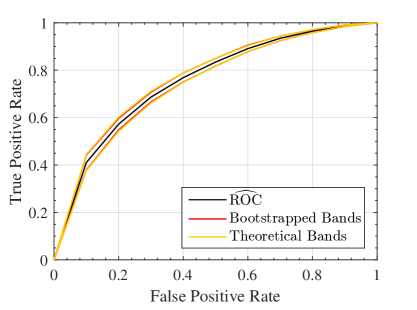
Figure 3: Theoretical and Bootstrapped Confidence Bands of the ROC Curve

In future work we plan to conduct a full scale Monte Carlo exercise where the above simulation is repeated numerous times and empirical coverage frequencies are compared with nominal coverage probabilities.

4 AUC and Model Comparison and Selection

When the ROCs of two potentially misspecified propensity score models cross each other, the area under the ROC curve (AUC) provides a heuristic crterion for model selection in the machine learning literature. A formal statistical comparison between the AUCs of estimated ROCs requires deriving their asymptotic distributions. This section undertakes such a task for parametric propensity score models. First, we investigate how the AUCs can be used to obtain parameter estimates. Second, we derive the asymptoic distribution of sample AUCs based on estimated parameters. Lastly, these results are used to provide model selection tests and model selection criterion.

4.1 Maximal AUC Estimator

The parameters $\theta$ in $p\left(X,\theta\right)$ with parameters $\theta$ are typically estimated by optimizing criterion (or loss) functions such as the log likelihood (MLE or cross-entropy), or MSE (weighted or unweighted least square loss). The AUC (Area under Curve) is an alternative criterion choice to cross-entropy and MSE. We show that the maximum AUC estimator is mathematically equivalent to the maximum rank correlation estimator of Sherman (1993). While it may be less efficient than MLE under correct specification, it allows for certain degrees of robustness, and is still consistent and asymptotically normal for a semiparametric single index model.

The sample AUC corresponding to $\theta$ is given by

$$\begin{split}\text{SAUC}\left(\theta\right)=\int\hat{\beta}_{\theta}\left(\alpha\right)d\alpha=\int\hat{\beta}_{\theta}\left(\hat{\alpha}_{\theta}^{-1}\left(\hat{\alpha}_{\theta}\right)\right)\mathrm{d}\hat{\alpha}_{\theta}=\int\hat{\beta}_{\theta}\left(c\right)\frac{\mathrm{d}\hat{\alpha}_{\theta}\left(c\right)}{\mathrm{d}c}\mathrm{d}c\end{split}$$

where

$$\begin{split}\hat{\beta}_{\theta}\left(c\right)=&\frac{1}{\hat{p}}\frac{1}{n}\sum_{i=1}^{n}\mathds{1}\left(p\left(x_{i},\theta\right)>c\right)y_{i},\quad\text{and}\\ \hat{\alpha}_{\theta}\left(c\right)=&\frac{1}{1-\hat{p}}\frac{1}{n}\sum_{j=1}^{n}\mathds{1}\left(p\left(x_{j},\theta\right)>c\right)\left(1-y_{j}\right).\end{split}$$

Using the notion of Dirac functions, $\mathrm{d}\mathds{1}\left(p\left(x_{j},\theta\right)>c\right)/\mathrm{d}c=\delta_{p\left(x_{j},\theta\right)}\left(c\right)$, we can write

$$\begin{split}\text{SAUC}\left(\hat{\theta}\right)=\frac{1}{n^{2}\hat{p}\left(1-\hat{p}\right)}\sum_{i=1}^{n}\sum_{j=1}^{n}\mathds{1}\left(p\left(x_{i},\hat{\theta}\right)>p\left(x_{j},\hat{\theta}\right)\right)y_{i}\left(1-y_{j}\right)\end{split}$$ (10)

This takes the form of a U-process, which is $\sqrt{n}$ consistent and converges asymptotically to a Gaussian process (Sherman (1993) and Hoeffding et al. (1948)).

The sample AUC converges to a population AUC, defined as

$$\begin{split}\mathrm{PAUC}\left(\theta\right)=\int\beta_{\theta}\left(\alpha\right)d\alpha=\int\beta_{\theta}\left(\alpha_{\theta}^{-1}\left(\alpha_{\theta}\right)\right)\mathrm{d}\alpha_{\theta}=\int\beta_{\theta}\left(c\right)\frac{\mathrm{d}\alpha_{\theta}\left(c\right)}{\mathrm{d}c}\mathrm{d}c\end{split}$$

such that

$$\begin{split}\beta_{\theta}\left(c\right)=&\frac{1}{p}\int\mathds{1}\left(p\left(x,\theta\right)>c\right)p\left(x\right)f\left(x\right)\mathrm{d}x\quad\text{and}\\ \alpha_{\theta}\left(c\right)=&\frac{1}{1-p}\int\mathds{1}\left(p\left(x,\theta\right)>c\right)\left(1-p\left(x\right)\right)f\left(x\right)\mathrm{d}x.\end{split}$$

Using the notion of Dirac functions again, we compute that

$$\begin{split}\text{PAUC}\left(\theta\right)=\frac{1}{p\left(1-p\right)}\iint\mathds{1}\left(p\left(x,\theta\right)>p\left(w,\theta\right)\right)p\left(x\right)\left(1-p\left(w\right)\right)f\left(x\right)f\left(w\right)\mathrm{d}x\mathrm{d}w.\end{split}$$ (11)

This integral would be maximized with respect to the indicator function if the indicator is turned on whenever $p\left(x\right)\left(1-p\left(w\right)\right)>p\left(w\right)\left(1-p\left(x\right)\right),$ equivalently or whenever $p\left(x\right)>p\left(w\right)$. Under correct specification, this can obviously be achieved when $\theta=\theta_{0}$, where $p\left(x,\theta_{0}\right)=p\left(x\right)>p\left(w\right)=p\left(w,\theta_{0}\right).$ Therefore, by standard M-estimator arguments (e.g. Newey and McFadden (1994)) the maximum AUC estimator is consistent under correct specification and suitable sample regularity conditions.

4.2 Single Index Model

A common semiparametric specification of $p\left(x_{i},\theta\right)$ is a single index model, where $p\left(x_{i},\theta\right)=\Lambda\left(x_{i}^{\prime}\beta\left(\theta\right)\right)$ and $\Lambda\left(\cdot\right)$ is strictly increasing but may be unknown. In this case,

$$\begin{split}\text{SAUC}\left(\theta\right)=\frac{1}{n^{2}\hat{p}\left(1-\hat{p}\right)}\sum_{i=1}^{n}\sum_{j=1}^{n}\mathds{1}\left(x_{i}^{\prime}\beta\left(\theta\right)>x_{j}^{\prime}\beta\left(\theta\right)\right)\mathds{1}\left(y_{i}>y_{j}\right)\end{split}$$

since $\mathds{1}\left(y_{i}>y_{j}\right)=y_{i}\left(1-y_{j}\right)$ for binary $y_{i},y_{j}$. As in Sherman (1993) $\beta\left(\theta\right)=\left(1,\theta\right)$ in order to reduce the dimension of the parameter space by $1$ since $\beta$ is only identified up to a multiplicative factor.

This is exactly the maximum rank correlation estimator of Sherman (1993). The theoretical consistency of $\hat{\theta}\overset{\mathbb{P}}{\rightarrow}\theta_{0}$ only requires that $\theta_{0}$ is the only point in $\theta\in\Theta$ such that

$$\begin{split}x^{\prime}\beta\left(\theta\right)>w^{\prime}\beta\left(\theta\right)\quad\text{if and only if}\quad p\left(x\right)>p\left(w\right),\quad\forall x,w.\end{split}$$

Sherman (1993) develops the asymptotic properties of $\hat{\theta}$ and shows that $\sqrt{n}\left(\hat{\theta}-\theta_{0}\right)$ is asymptotically linear under the assumption of a correctly specified model of the form

$$\begin{split}y_{i}=D\left(g\left(x_{i}^{\prime}\beta\left(\theta\right),\epsilon_{i}\right)\right)\end{split}$$

where $g\left(\cdot,\cdot\right)$ is smooth and strictly increasing in both arguments, $D\left(\cdot\right)$ is weakly increasing, and $\epsilon_{i}\perp x_{i}$. However, the high level framework in Sherman (1993) is readily generalizable to allow for potential misspecification where the single index assumption does not hold.

Under misspecification we assume that sufficient regularity conditions hold such that a pseudo true value is uniquely defined in the population:

$$\begin{split}\theta^{*}=\arg\max_{\theta\in\Theta}\mathbb{E}\left[\mathds{1}\left(X_{i}^{\prime}\beta\left(\theta\right)>X_{j}^{\prime}\beta\left(\theta\right)\right)\mathds{1}\left(Y_{i}>Y_{j}\right)\right].\end{split}$$

We note the sections 1-5 of Sherman (1993) hold generally without the single index assumption. Only section 6 of Sherman (1993), the exact form of the asymptotic variance, the influence function, and the Hessian matrix, need to be generalized to allow for misspecification. The appendix provides these general forms, which specialize to Section 6 of Sherman (1993) under the single index model, and verifies that

$$\begin{split}\sqrt{n}\left(\hat{\theta}-\theta^{*}\right)=\frac{1}{\sqrt{n}}\sum_{i=1}^{n}\kappa_{i}+o_{P}\left(\frac{1}{\sqrt{n}}\right),\end{split}$$ (12)

where $\hat{\theta}=\arg\max_{\theta\in\Theta}\text{SAUC}\left(\theta\right)$. Note that (12) generally holds for $\hat{\theta}$ obtained from optimizing many criterion functions such as the KLIC, with a corresponding influence function $\kappa_{i}$ that is dependent on the criterion function.

The single index model is semiparametric and does not require knowledge of the transformation function $\Lambda\left(\cdot\right)$. If $\Lambda\left(\cdot\right)$ is known (so is $p\left(x,\theta\right)$) and the model is fully parametric, the AUC can alternatively be estimated by the sample analog of (11):

$$\begin{split}\text{SAUC}_{p}\left(\hat{\theta}\right)=\frac{1}{\hat{p}\left(1-\hat{p}\right)}\frac{1}{n^{2}}\sum_{i=1}^{n}\sum_{j=1}^{n}\mathds{1}\left(p\left(x_{i},\hat{\theta}\right)>p\left(x_{j},\hat{\theta}\right)\right)p\left(x_{i},\hat{\theta}\right)\left(1-p\left(x_{j},\hat{\theta}\right)\right).\end{split}$$ (13)

When $p\left(x_{j},\hat{\theta}\right)$ is correctly specified and when $\hat{\theta}$ is obtained by MLE, (13) is more efficient than (10) for estimating (11). The asymptotic efficiency gain can be analytically calculated.

4.3 Asymptotic Normality of AUC

This section makes further use of the U-process convergence results in Sherman (1993) to derive the influence function representation and asymptotic normality of the sample estimated AUC. These results are used in the next section to provide the basis for AUC-based model comparison tests and model selection criteria. Previous works by Hanley and McNeil (1982) and Hsieh et al. (1996) that treated the SAUC as two-sample U-statistics (see Lehmann (2004)) do not account for the parameter estimation uncertainty and the random denominator containing $\hat{p}=1/n\sum^{n}_{i=1}y_{i}$ as derived in Section 4.1.

Let $z_{i}=\left(x_{i},y_{i}\right)$ and $\omega\left(z_{i},z_{j},\theta\right)=\mathds{1}\left(p\left(x_{i},\theta\right)>p\left(x_{j},\theta\right)\right)\mathds{1}\left(y_{i}>y_{j}\right)$. Recall that

$$\begin{split}\hat{A}=&\text{SAUC}\left(\hat{\theta}\right)=\frac{1}{n^{2}\hat{p}\left(1-\hat{p}\right)}\sum^{n}_{i=1}\sum^{n}_{j=1}\omega\left(z_{i},z_{j},\hat{\theta}\right),\\ A=&\text{PAUC}\left(\theta^{*}\right)=\frac{1}{p\left(1-p\right)}E\omega\left(z_{i},z_{j},\theta^{*}\right).\end{split}$$ (14)

The goal is to obtain the linear representation and limiting distribution of $\hat{A}$:

$$\begin{split}\sqrt{n}\left(\hat{A}-A\right)=\frac{1}{\sqrt{n}}\sum_{i=1}^{n}\xi_{i}+o_{\mathbb{P}}\left(\frac{1}{\sqrt{n}}\right),\quad\sqrt{n}\left(\hat{A}-A\right)\overset{d}{\longrightarrow}N\left(0,Var\left(\xi_{i}\right)\right).\end{split}$$ (15)

To obtain (15) we begin by writing

$$\begin{split}\sqrt{n}\left(\hat{A}-A\right)=\frac{\sqrt{n}}{n^{2}\hat{p}\left(1-\hat{p}\right)}\sum^{n}_{i=1}\sum^{n}_{j=1}\left(\omega\left(z_{i},z_{j},\hat{\theta}\right)-A\hat{p}\left(1-\hat{p}\right)\right).\end{split}$$

Note that $\hat{p}\left(1-\hat{p}\right)\overset{\mathbb{P}}{\longrightarrow}p\left(1-p\right),$ it suffices to show that for some $\zeta_{i}$

$$\begin{split}\frac{\sqrt{n}}{n^{2}}\sum^{n}_{i=1}\sum^{n}_{j=1}\left(\omega\left(z_{i},z_{j},\hat{\theta}\right)-A\hat{p}\left(1-\hat{p}\right)\right)=\frac{1}{\sqrt{n}}\sum_{i=1}^{n}\zeta_{i}+o_{\mathbb{P}}\left(\frac{1}{\sqrt{n}}\right).\end{split}$$

By arguments of Slutsky’s lemma, then

$$\begin{split}\sqrt{n}\left(\hat{A}-A\right)=\frac{1}{\sqrt{n}}\sum_{i=1}^{n}\frac{1}{p\left(1-p\right)}\zeta_{i}+o_{\mathbb{P}}\left(\frac{1}{\sqrt{n}}\right).\overset{d}{\longrightarrow}N\left(0,\frac{Var\left(\zeta_{i}\right)}{p^{2}\left(1-p\right)^{2}}\right).\end{split}$$

Noting that

$$\begin{split}\hat{p}\left(1-\hat{p}\right)&=\frac{1}{n}\sum^{n}_{i=1}y_{i}-\frac{1}{n^{2}}\sum^{n}_{i=1}\sum^{n}_{j=1}y_{i}y_{j}=\frac{1}{n^{2}}\sum^{n}_{i=1}\sum^{n}_{j=1}\left[y_{i}\left(1-y_{j}\right)\right],\end{split}$$

and that $\hat{p}\left(1-\hat{p}\right)=\frac{1}{n^{2}}\sum^{n}_{i=1}\sum^{n}_{j=1}\left(\hat{p}\left(1-\hat{p}\right)\right)$, we can rewrite as

$$\begin{split}\frac{\sqrt{n}}{n^{2}}\sum^{n}_{i=1}\sum^{n}_{j=1}\left(\omega\left(z_{i},z_{j},\hat{\theta}\right)-A\hat{p}\left(1-\hat{p}\right)\right)=\frac{\sqrt{n}}{n^{2}}\sum^{n}_{i=1}\sum^{n}_{j=1}\underbrace{\left[\omega\left(z_{i},z_{j},\hat{\theta}\right)-Ay_{i}\left(1-y_{j}\right)\right]}_{\eta\left(z_{i},z_{j},\theta\right)},\end{split}$$

where, using the definition of $\omega\left(z_{i},z_{j},\theta\right)$ and note that $\mathds{1}\left(y_{i}>y_{j}\right)=y_{i}\left(1-y_{j}\right)$,

$$\begin{split}\eta\left(z_{i},z_{j},\theta\right)=\left(\mathds{1}\left(p(x_{i},\theta)>p\left(x_{j},\theta\right)\right)-A\right)y_{i}\left(1-y_{j}\right)\end{split}$$

If we define,

$$\begin{split}\hat{Q}\left(\theta\right)=\frac{1}{n^{2}}\sum^{n}_{i=1}\sum^{n}_{j=1}\eta\left(z_{i},z_{j},\theta\right)\quad\text{and}\quad Q\left(\theta\right)=\mathbb{E}\left[\eta\left(z_{i},z_{j},\theta\right)\right]\equiv 0,\end{split}$$

then we can invoke the U-process stochastic equicontinuity results in Sherman (1993):

$$\begin{split}\hat{Q}\left(\hat{\theta}\right)-\hat{Q}\left(\theta^{*}\right)-Q\left(\hat{\theta}\right)+Q\left(\theta^{*}\right)=o_{\mathbb{P}}\left(\frac{1}{\sqrt{n}}\right),\end{split}$$

such that, using (12), where $\hat{\theta}$ is obtaining from optimizing a general criterion function that may or may not be the SAUC,

$$\begin{split}\hat{Q}\left(\hat{\theta}\right)-Q\left(\theta^{*}\right)=&\hat{Q}\left(\theta^{*}\right)-Q\left(\theta^{*}\right)+Q\left(\hat{\theta}\right)-Q\left(\theta^{*}\right)+o_{\mathbb{P}}\left(\frac{1}{\sqrt{n}}\right)\\ =&\frac{1}{n^{2}}\sum^{n}_{i=1}\sum^{n}_{j=1}\eta\left(z_{i},j_{j},\theta^{*}\right)+\frac{\partial}{\partial\theta}Q\left(\theta^{*}\right)\frac{1}{n}\sum_{i=1}^{n}\kappa_{i}+o_{\mathbb{P}}\left(\frac{1}{\sqrt{n}}\right)\\ =&\frac{1}{n}\sum_{i=1}^{n}\left(\eta_{1}\left(z_{i},\theta^{*}\right)+\eta_{2}\left(z_{i},\theta^{*}\right)+\frac{\partial}{\partial\theta}Q\left(\theta^{*}\right)\kappa_{i}\right)+o_{\mathbb{P}}\left(\frac{1}{\sqrt{n}}\right).\end{split}$$

where by Hájek projection,

$$\begin{split}\eta_{1}\left(z_{i},\theta\right)=\mathbb{E}_{z_{j}}\left[\eta\left(z_{i},z_{j},\theta\right)\right],\quad\eta_{2}\left(z_{j},\theta\right)=\mathbb{E}_{z_{i}}\left[\eta\left(z_{i},z_{j},\theta\right)\right],\end{split}$$

We therefore conclude that (15) holds with

$$\begin{split}\zeta_{i}=\eta_{1}\left(z_{i},\theta^{*}\right)+\eta_{2}\left(z_{i},\theta^{*}\right)+\frac{\partial}{\partial\theta}Q\left(\theta^{*}\right)\kappa_{i}\quad\text{and}\quad\xi_{i}=\frac{1}{p\left(1-p\right)}\zeta_{i}.\end{split}$$

If $\hat{\theta}$ is the maximum AUC estimator, then $\frac{\partial}{\partial\theta}Q\left(\theta^{*}\right)=0$, so that the last term vanishes from $\zeta_{i}$, in which case parameter estimation uncertainty vanishes asymptotically in first order. On the other hand, parameter uncertainty is first order important when $\hat{\theta}$ optimizes another criterion function that differs from the AUC.

(15) can be used for analytically constructing asymptotic tests by estimating sample analogs of $\xi_{i}$, or for justifying the validity of resampling procedures.

The results in the previous three sections assume that the entire sample is used for both parameter and AUC estimation, or that a fixed sample splitting scheme is employed. A random split of the sample into parameter estimation and AUC calculation can be accommodated by introducing random indicators $D_{i}$, such that $D_{i}=1$ denotes the parameter estimation subsample and $D_{i}=0$ denotes the AUC calculation subsample. Previous results can be readily generalized by replacing (12) with $D_{i}\kappa_{i}$, the double summation in (14) with

$$\begin{split}\sum^{n}_{i=1}\sum^{n}_{j=1}\left(1-D_{i}\right)\left(1-D_{j}\right)\omega\left(z_{i},z_{j},\hat{\theta}\right),\end{split}$$

and corresponding changes in related influence functions. In general, sample splitting increases the variance of the estimated AUC.

4.4 Model Comparison Tests and Model Selection Criteria

Following a vast literature in econometrics and statistics, results derived in the last two sections provide the basis for constructing model selection tests and forming model selection criteria. This section provides a brief overview.

When at least one model is correctly specified, any criterion function (such as cross-entropy or KLIC) combined with suitable penalization can be used to select the most parsimonious correct model, or to be used to form specification test statistics for individual models. Under the assumption of potentially misspecification of all models under consideration, the end result may depend on the choice of criterion functions even asymptotically. KLIC or MSE are popular choices in econometrics and statistics, while in computer science, AUC has been advocated for this purpose. We therefore focus on the AUC.

If the AUC is used as the criterion functions both for estimating the parameters of the competing models and for testing and selecting between models, then the generaly results from Vuong (1989), and Hong et al. (2003), apply. It is also possible that a different criterion function, such as cross entropy, is used to estimate parameters before the use of the AUC criterion function to compare or select between competing models. The sample can be split between estimation and model testing and selection, or the same sample can be employed for both purposes. Both cases can be handled similarly using asymptotic linear representations.

Consider two competing models with parameters $\theta$ and $\vartheta$, and corresponding sample AUCs $\hat{A}_{1}\left(\hat{\theta}\right)$ and $\hat{A}_{2}\left(\hat{\vartheta}\right)$, then it follows from (15) that

$$\begin{split}\hat{A}_{1}\left(\hat{\theta}\right)-\hat{A}_{2}\left(\hat{\vartheta}\right)=\left(A_{1}\left(\theta^{*}\right)-A_{2}\left(\vartheta^{*}\right)\right)+\frac{1}{n}\sum_{i=1}^{n}\left(\xi_{i}^{1}-\xi_{i}^{2}\right)+o_{\mathbb{P}}\left(\frac{1}{\sqrt{n}}\right).\end{split}$$ (16)

A test of the null hypothesis of $A_{1}\left(\theta^{*}\right)=A_{2}\left(\vartheta^{*}\right)$ between two nonnested models can rely asymptotically on the nondegenerate distribution of $\xi_{i}^{1}-\xi_{i}^{2}$. For nested models where $\xi_{i}^{1}-\xi_{i}^{2}$ may be degenerate, a second order expansion of the parameter estimation uncertainty may be required to obtain a nondegenerate limit distribution.

A model selection criterion typically takes the form of $\hat{A}\left(\hat{\theta}\right)+\kappa_{n}\dim\left(\theta\right)$ which penalizes the number of parameters in order to be parsimonious. Consistent model selection, in the sense of choosing the most parsimonious and best fit model with probability model, is achieved by requiring the penalization term $\kappa_{n}$ to satisfy $\kappa_{n}\rightarrow 0$ and $\sqrt{n}\kappa_{n}\rightarrow\infty$. The latter requirement can be relaxed to $n\kappa_{n}\rightarrow\infty$ between nested models.

4.5 Simulation Results

We continue to use the data set of Section 3.3 as an illustrating example. First the true model coefficients (i.e. 1 and -0.5) are assumed to be known and are used to estimate the theoretical asymptotic standard deviation of SAUC based on analytic sample analogs as 0.00632. We also bootstrap test data set for 1,000 times, calculating AUCs for each iteration at the true coefficients. The bootstrapped standard deviation of the SAUC thus obtained is 0.00629, which accords with the analytic estimate of the theoretical value in the absence of parameter estimation uncertainty and random sample splitting.

Next we incorporate parameter estimation uncertainty. Table 2 lists the estimated coefficients of the logit model (with a fixed intercept as 0) using a maximal likelihood approach and a maximum AUC (MAUC) approach using the training data set. We estimate the standard deviation of the two coefficients in the logit model using 1000 bootstrap repetitions of the data sample. The coefficient estimates are both close to the true model parameters, but slightly different. For the first coefficient, the point estimate of MAUC is closer to the true parameter than MLE is, but with a larger standard deviation estimate. The reverse is true for the second coefficient. Finally we report the AUC estimates using the mean of the bootstrap based on MLE and MAUC, and their bootstrap standard deviations. The AUC estimate based on MAUC is slightly larger than that based on MLE. The bootstrap standard deviations are essentially identical, and show that a substantial component (more than 50%) of the standard deviation is due to the uncertainty from parameter estimation and from random sample splitting.

Table 2: Parameter Estimations using MLE and Maximal AUC Approaches

	True Model	MLE	Maximal AUC
X1 (mean)	1	1.0045	0.9992
X1 (std)	NA	0.0178	0.0381
X2 (mean)	-0.5	-0.5502	-0.5688
X2 (std)	NA	0.0301	0.0184
AUC (mean)	0.7683	0.7689	0.7694
AUC (std)	NA	0.0151	0.0151

Table 3 reports an AUC-based model selection exercise between two misspecfied models given the data generating process in section 3.3. The first (M1) is a logit model with $p(X_{1})=\frac{\exp(\theta_{1}X_{1})}{1+\exp(\theta_{1}X_{1})}$; the model (M2) is a logit model with $p(X_{2})=\frac{\exp(\theta_{2}X_{2})}{1+\exp(\theta_{2}X_{2})}$. We bootstrap the whole data set 1,000 times. In each iteration, we randomly partition the whole data set in two halves, one as the training set for parameter estimation and the other one as the test set for AUC calculation. We then estimate M1 and M2 separately and obtain their AUCs (A1 and A2) accordingly. Finally, we calculate the mean AUC spreads and corresponding standard deviation, using both the theoretical first order approximation in (16) and using bootstrapping. We obtain a significant $z$ score: $z=\frac{\hat{A}_{1}\left(\hat{\theta}\right)-\hat{A}_{2}\left(\hat{\vartheta}\right)}{std(\hat{A}_{1}\left(\hat{\theta}\right)-\hat{A}_{2}\left(\hat{\vartheta}\right))}$, which rejects the null hypothesis that M1 is equivalent to M2 in favor of the directional alternative hypothesis that M1 is a better model.

Table 3: Model Selection

	Bootstrap	Theoretical
A1 (mean)	0.7341	0.7314
A2 (mean)	0.6214	0.6191
A1-A2 (mean)	0.1127	0.1124
A1-A2 (std)	0.0102	0.0103

As in section 3.3, a full scale Monte Carlo simulation to gauge the bias, variance and mean square errors of competing estimators is left for future investigation.

5 Human Decisions and Machine Decisions

In a dataset, we typically observe a sample of the triples $\left(Y_{i},D_{i},X_{i}\right),i=1,\ldots,n$, where $Y_{i}$ is the label outcome variable such as whether the birth is normal or defect, $D_{i}$ is the predicted value for $Y_{i}$ by a human decision maker such as a doctor, and $X_{i}$ is the set of features that can be used to predict $Y_{i}$ or $D_{i}$. A machine learning algorithm learns a model $\hat{p}\left(X_{i}\right)$ using the training subset of $Y_{i},X_{i}$, and forms a ROC curve based on the prediction rules $\hat{Y}_{i}=1\left(\hat{p}\left(X_{i}\right)>c\right)$ when $c$ varies between $0$ and $1$.

An aggregate human TPR/FPR pair is calculated using $Y_{i},D_{i},i=1,\ldots,n$ as

$$\begin{split}\text{TPR}=\frac{\sum_{i=1}^{n}Y_{i}D_{i}}{\sum_{i=1}^{n}Y_{i}}\quad\text{and}\quad\text{FPR}=\frac{\sum_{i=1}^{n}\left(1-Y_{i}\right)D_{i}}{\sum_{i=1}^{n}\left(1-Y_{i}\right)}\end{split}$$

A popular approach to benchmark the performance of human (doctor) decisions is to see whether the (TPR, FPR) pair lies above or below the AI ROC curve. That the human (TPR, FPR) pair lies below machine ROC is interpreted as evidence that AI dominates human decision making, and vice versa. In the former case, there exists a point on the machine ROC with the same FPR as human decision makers but higher TPR than human decision makers. Alternatively, there exists another point on the machine ROC with the same TPR as human decision makers but with lower FPR. No point on the machine ROC is dominated by the human (TPR, FPR) pair in the sense of having lower values in both ratios. See, for example, Kleinberg et al. (2018).

These interpretations are based on the strong assumption that doctors employ the same model and use the same cutoff value $c$ to form predictions. That the machine generated ROC dominates human (TPR, FPR) pair is then attributed to doctors using less information or a misspecified model. In reality, both information and incentive heterogeneity are likely to be present among doctors. The information set that humans base their diagnosis on may differ from the feature set used in the machine learning algorithm. For example, doctors may have observed patients’ complexion and discovered other information when conversing with patients, which are not recorded as features in the data set. Furthermore, even if doctors employ the same model using the same information set, they might differ in the cutoff value $c$ because of the difference in their perception regarding the tradeoff between type I and type II errors. This section explores how heterogeneous incentive and information asymmetry complicate the comparison between machines and humans.

Our data set has a panel structure where multiple observations are available for each doctor, such that $n$ (TPR, FPR) pairs can be drawn for each of the $n$ doctors. The panel structure does not eliminate concerns about information and incentive heterogeneity, and is subject to the criticism based on Jensen’s inequality outlined in section 1. However, it does provide a useful source of identification that we will explore in this section.

Furthermore, using $D_{i},X_{i},i=1,\ldots,n$, we can train a machine learning model for predicting human decisions $D_{i}$ based on the features $X_{i}$, and generate a probabilistic estimate of $q\left(X_{i}\right)=\mathbb{P}\left(D_{i}=1|X_{i}\right)$. In other words, $q\left(X_{i}\right)$ is a model of “predictded doctors”. Next, we can use $q\left(X_{i}\right)$ to forecast $Y_{i}$ based on the rules $\hat{Y}_{i}=1\left(q\left(X_{i}\right)>c\right)$ where $c$ varies between $0$ and $1$, and form a resulting ROC curve. This will be called the “predicted doctor ROC”. The rest of this section explores the relation between the aggregate (TPR, FPR) pair, the machine learned ROC (MROC), and the predicted doctor ROC (PROC) under different incentive and information structures. We maintain the assumption that the machine can accurately learn the correct $p\left(X_{i}\right)=\mathbb{P}\left(Y=1|X_{i}\right)$.

5.1 The PROC with homogeneous information and incentive

First we note that regardless of the information and incentive structure, MROC and PROC might coincide even when $p\left(X\right)$ and $q\left(X\right)$ differ. In particular, whenever $q\left(x\right)$ is a strictly increasing transformation of $p\left(x\right)$, their corresponding ROCs must coincidence, because by monotonicity, there exists a function $\bar{c}\left(t\right)$ such that $q\left(x\right)>t$ if and only if $p\left(x\right)>\bar{c}\left(t\right)$. Therefore a point on the MPOC corresponding to threshold $t$ maps into a point on the PROC corresponding to threshold $\bar{c}\left(t\right)$. Lemma A.3 establishes the converse. For example, $q\left(x\right)$ is a monotonic transformation of $p\left(x\right)$ when they are both monotonic functions of a scalar $x$.

Next consider a situation where humans use the same model based on the observed $X$, and are incentive homogeneous by using the same cutoff value $c_{0}$. In other words, for some $\bar{p}\left(x\right)$, $D_{i}=1\left(\bar{p}\left(X_{i}\right)\geq c_{0}\right)$. Then the humans’ ROC curve shrink to a TPR/FPR singleton, which also coincides with the aggregate humans’ TPR/FPR pair. $\bar{p}\left(x\right)$ can be misspecified and need not be related to the true $p\left(x\right)$. For example, Figure 4 is based on a model in which $x\sim Uniform\left(0,1\right)$, $p\left(x\right)=x$, but humans mistakenly think that $\bar{p}\left(x\right)=|\sin\left(10x\right)|$. The homogeneous humans’ decision rule is $\hat{Y}=\mathds{1}\left(\bar{p}\left(x\right)>.5\right)$. Lemma A.4 suggests that the PROC reduces to a single point that is also the humans’ aggregate TPR/FPR pair, both of which lie strictly below the MROC. It will be on the MROC when $\bar{p}\left(\cdot\right)=p\left(\cdot\right)$, or when $\bar{p}\left(\cdot\right)$ is an increasing transformation of $p\left(\cdot\right)$. Empirically, it is very unlikely that neither information nor incentive heterogeneity is present.

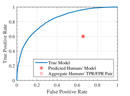
Figure 4: (Misspecified) Homogeneous Information

5.2 Incentive Heterogeneity

This section considers incentive heterogeneity (only, without information asymmetry). Specifically, suppose all humans have access to the same information of $X$, and they know the true $p\left(X\right)$. However, each human employs their own idiosyncratic fixed cost for the optimal tradeoff between true positives and false positives, implying that humans are heterogeneous in the cutoff values that they use in making predictions.

Moreover, each individual decision maker may not have a constant preference, and may change her cutoff threshold $c$ based on observed features. In this case, each decision maker does not need to be represented by a single point on the ROC curve. For example, Currie and MacLeod (2017) find that patients’ demand on C-section delivery can influence doctor’s decision. If certain groups of patients with similar characteristics have similar C-section demands, the cutoff value $c$ will depend on these characteristics of patients $x$. Chandra and Staiger (2011) find that hospitals treat similar patients differently due to consideration of commercial benefits. Therefore $c$ depends on both hospitals and the location of patients. In the context of our empirical application in section 6, suppose $x$ is a one dimensional variable denoting age. While the probability of birth defect is likely to be strictly increasing in $x$, doctors may place a high weight on diagnosing normal older couples correctly: they would not want older but normal couples to forgo any chance of conception. Then $c\left(x\right)$ can also be strictly increasing in $x$. As a result, doctors may tend to diagnose younger couples as abnormal but older couples as normal. The next subsection illustrates this in more details.

If this type of incentive heterogeneity exists across the sample of decision makers, or within each individual, the aggregate TPR/FPR pair can lie below the optimal ROC curve, or even below the 45 degree line, even if humans have better information processing capacities than machines. Lemma A.2 provides a formal proof.

5.2.1 Cutoff Thresholds

If the loss functions $C_{0R}$ and $C_{1A}$ for a decision maker in (LABEL:C0C1) depends on observed features $x$ as proposed by Elliott and Lieli (2013), (3) also shows that $c$ is no more a constant, but instead depends on $x$.

Moreover, the predicted humans’ ROC curve may also differ from the true (and optimal) MROC curve, even if humans know the true $p\left(X\right)$. For example, let $X\sim Uniform\left(0,1\right)$, $p\left(X\right)=X$, $\eta\sim Uniform\left(0,1\right)$, $Y=\mathds{1}\left(p\left(X\right)>c\left(X,\eta\right)\right)$,

$$\begin{split}c(X,\eta)=\eta\left[\left(X<.5\right)+\left(X>.75\right)\right]+\eta X^{2}\left(.5<X<.75\right).\end{split}$$

So that the “predicted human” becomes

$$\begin{split}\bar{p}\left(x\right)=x\left[\left(x<.5\right)+\left(x>.75\right)\right]+1/x\left(.5<x<.75\right).\end{split}$$

Figure 5 plots the PROC curve of this example, part of which lies strictly below the MROC.

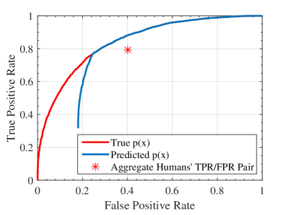
Figure 5: Incentive Heterogeneity, Incentive Distributions (Cutoff Threshold) Dependent on Features

Incentive heterogeneity may be controlled by conditioning on a subset of the features. If we postulate that the features $x$ can be partitioned into $x_{1},x_{2}$ where the cutoff function $c\left(x_{2}\right)$ only depends on $x_{2}$, then we can conduct the analysis conditional on $x_{2}$, and construct both ROC curves and the humans’ pairs across $x_{1}$ for each given $x_{2}$ to examine their relations. This requires plotting multiple conditional ROCs across $x_{1}$, for each level of $x_{2}$, to see if humans’ pairs of TPR/FPR conditional on $x_{2}$ fall on each of the corresponding (to each $x_{2}$) ROC curves. If $x_{2}$ takes a small number of finite values, the analysis can be done for each value of $x_{2}$. If $x_{2}$ is continuous, then some type of local smoothing will be needed to generate these graphs. Unless $p\left(x_{1},x_{2}\right)$ does not depend on $x_{2}$, if we had plotted the aggregate ROC corresponding to $p\left(x_{1},x_{2}\right)$ jointly in $x_{1},x_{2}$, it will lie above the individual ROCs corresponding to each level of $x_{2}$. As such, each of humans’ PTPR/PFPR pairs might still lie underneath the aggregate ROC due to incentive heterogeneity in decision making.

5.2.2 Uncover Incentive Heterogeneity from Data

A natural follow up question is the extent to which individual heterogeneity in decision making can be recovered from empirical data. To be more specific, assume that humans have the same and correct information as the machine learning algorithm does, i.e. have knowledge of the correct propensity score function $p\left(X\right)$. In this subsection, we temporarily define the cutoff value as $S$ (instead of $c$), which is a random variable whose distribution may depend on $X$, with a conditional cumulative distribution function denoted as $F_{S|X}\left(S|x\right)$. First of all, from the empirical data, a learning algorithm recovers an estimate of $p\left(X\right)$ using the real outcome as the label. Then using the decision of humans as the label, a learning algorithm can recover

$$\begin{split}q\left(x\right)=\mathbb{P}\left(S<p\left(x\right)|x\right)=F_{S|X}\left(p\left(x\right)|x\right).\end{split}$$

Given a data set of $X_{i}$, $p_{i}=p\left(X_{i}\right)$, and $q_{i}=q\left(X_{i}\right)$, this translates into a relation of

$$\begin{split}q_{i}=h\left(p_{i},X_{i}\right)\quad\text{where}\quad h\left(p,x\right)=F_{S|X}\left(p,x\right).\end{split}$$

A supervised learning algorithm can be used to estimate $h\left(p,x\right)$ using $q_{i}$ as the label and the tuple of $\left(p_{i},X_{i}\right)$ as the features, and can be expected to perform well if $h\left(p,x\right)$ satisfies suitable regularity or continuity conditions. There are two applications of the learned $h\left(p,x\right)$ function. First, when $S$ is independent of $X$, where $q\left(X\right)=F_{S}\left(p\left(X\right)\right)$, $q_{i}$ is then a monotonically increasing transformation of $p_{i}$. Therefore, by testing for monotonicity, we can infer whether the distribution of the random threshold depends on observed features or not. Second, if a panel data set is available, by comparing $h\left(p,x\right)$ for different human decision makers, we can explicitly recover the incentive heterogeneity of their decision making.

5.3 Information Asymmetry

Next we abstract away from incentive heterogeneity and focus on information asymmetry. Suppose that in addition to the observed features $X$, humans also make decision based on $U$, where $U$ is not observed by the researchers or the machine learning algorithm. For example, $U$ could be the facial complexion of the patient that the doctor observed during the day of the clinic visits. Let $p\left(X,U\right)=\mathbb{P}\left(Y=1|U,X\right)$.

Consider first a case where humans know the correctly specified propensity score $p\left(X,U\right)$, and use a homogeneous decision rule $\hat{Y}=\mathds{1}\left(p\left(X,U\right)>c\right)$. In this case, because $p\left(X,U\right)$ correctly uses more information than $p\left(X\right)$ does, the (unobserved) ROC formed by $p\left(X,U\right)$ lies strictly above the MROC formed by the machine’s propensity score

$$\begin{split}p\left(X\right)=\int p\left(X,U\right)f\left(U|X\right)\mathrm{d}U.\end{split}$$

Furthermore, the aggregate human TPR/FPR pair must lie on the ROC formed by $p\left(X,U\right)$, and hence above the machine’s MROC curve. Lemma A.5 provides the proof. Therefore, if humans are incentive homogenous in decision making, and their aggregate TPR/FPR pair is below the machine’s ROC curve, one can conclude that humans either do not know the true propensity score or use wrong information in making decisions.

Next, consider a situation in which the human has potentially more, but wrong information, and employs a misspecified model $\bar{p}\left(x,u\right)$. In this case, the predicted human’s ROC curve is defined by the ROC corresponding to the “pseudo” propensity score function:

$$\begin{split}\bar{p}\left(x\right)=\mathbb{E}_{U|X}\left[\mathds{1}\left(\bar{p}\left(X,U\right)>c\right)\right]=\int\mathds{1}\left(\bar{p}\left(X,U\right)>c\right)f\left(U|X\right)\mathrm{d}U\end{split}$$

which is likely to differ from $p\left(X\right)$. The implied PROC might coincide with the MROC, or might below it.

For example, let the true model be $p\left(x,u\right)=\exp(x)/\left(1+\exp(x)\right),$ but human decision maker uses the model, for $u$ uniformly distributed on $\left(0,1\right)$,

$$\begin{split}\bar{p}\left(x,u\right)=\frac{\exp(x+u)}{1+\exp(x+u)}.\end{split}$$

In this model, despite using the wrong information model, the predicted human’s propensity score $\bar{p}\left(x\right)=\mathbb{E}_{u}\left[\mathds{1}\left(\bar{p}\left(x,u\right)\geq c\right)\right]$ is a monotonic function of $x$, and therefore has a PROC curve based on $x$ that coincides with that of $p\left(x\right)$ (see Appendix A.3).

To generate divergence between the predicted humans’ PROC curve and the MROC curve from the true model, we would need to introduce either reverse monotonicity or nonmonotonicy between $\bar{p}\left(x\right)$ and $p\left(x\right)$, or multidimensional features $x$. If the human’s information model has the wrong sign in $x$:

$$\begin{split}\bar{p}\left(x,u\right)=\frac{\exp(-x+u)}{1+\exp(-x+u)}.\end{split}$$

Then the predicted humans’ PROC curve and the true MROC curve differ in Figure 6.

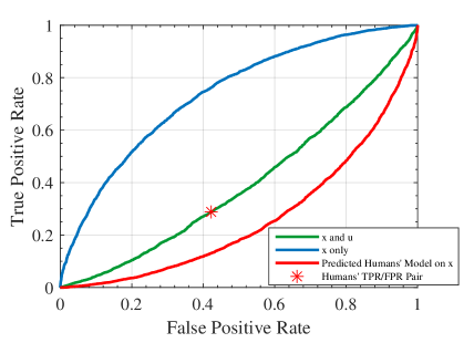
Figure 6: Misspecified Heterogeneous and Non-monotonic Information

Next consider a two dimensional feature case. Let the true model be

$$\begin{split}p\left(x_{1},x_{2},u\right)=\exp(x_{1}+x_{2})/(1+\exp(x_{1}+x_{2})),\quad x_{1}\sim N\left(0,1\right),\quad x_{2}\sim N\left(0,0.09\right).\end{split}$$

And let the human’s (wrong) information model be

$$\begin{split}\tilde{p}\left(x_{1},x_{2},u\right)=\exp(x_{1}-x_{2}+u)/(1+\exp(x_{1}-x_{2}+u)),\ \text{where }u\sim N\left(0,4\right),\end{split}$$

Then we observe ROC curves in Figure 7.

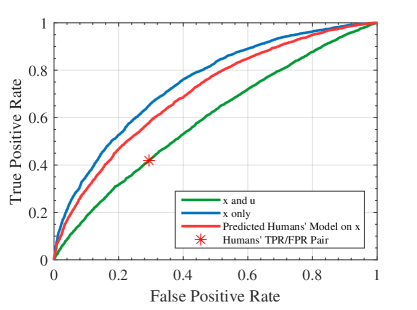
Figure 7: Misspecified Heterogeneous and Multi-dimensional Information

6 Application: Birth Defect Decisions

To motivate and empirically illustrate our theoretical discussion, we make use of a survey data set of high risk pregnancy diagnosis with more than a million observations as an application of our findings.

6.1 Data

Our data is derived from the National Free Pre-Pregnancy Checkups (NFPC) in Henan Province.The NFPC is a population-based health survey of reproductive-aged couples and was administered in China from January 1, 2014 to December 31, 2015 to expecting couples or couples who plan to have children. The data set include most of the information available to the doctor at the time of the diagnosis, including age and other demographic characteristic, results from medical examination and clinical test, individual and family history of diseases and drug use, pregnancy history, as well as separate lifestyle and other living environment information for both spouses. Altogether 282 features are available for each observation in the sample. The label of the data indicates whether the pregnancy outcome is normal (y = 0) or involves birth defects (y = 1). Of these samples, 4239(2.2%) couples have an adverse pregnancy outcome.

In addition, the data set also includes doctor’s pregnancy risk assessments. The doctors’ diagnosis is coded as 4 levels-0 for normal, 1 for high-risk in terms of female, 2 for high high-risk in terms of male, and 3 for high risk in terms of both female and male. Unless otherwise noted, we regard 1, 2, 3 of doctor’s assessment as a diagnosis of risky outcome, and 0 as a diagnosis of normal pregnancy outcome. A total of 20.2% of our sample was diagnosed as risky; overall, doctors achieve 78.58% average accuracy. The doctors’ general tendency to classify a large portion of normal birth as risky is suggestive of a high cost of false negatives relative to the false positives.

We exclude from the original data sample observations with missing information on pregnancy outcome, as well as those for which more than 50% of feature values are missing. The final data used in the current analysis includes 192551 couples, who are diagnosed by 1526 doctors.

6.2 Machine Learning Algorithm

We experiment with a number of machine learning binary classification algorithm including logistic regression, deep neural networks, and regression trees. For parametric models, deep neural networks can achieve good classification performance. Similar to the simulation experiment, we bootstrap the whole sample (100) times and draw the 95% confidence bands based on the bootstrapped ROC curves depicted in Figure 8. We used an 8:2 training set and test set partition. Note that there exist categorical features in the data. For example, the mother’s occupation is coded as 1 for the farmer, 2 for the factory worker, etc. Neural networks are not good at handling such structured data (Guo and Berkhahn (2016)). To address this issue we used an entities embedding method (Guo and Berkhahn (2016), Yang et al. (2015)) to map these features to embedded vectors that can be directly utilized by a neural network. We used a 5-layer fully-connected neural network for prediction, with 50, 50, 50, 50, 25 neurons per layer, and ReLU (Rectified Linear Unit) is used as the activation function. A dropout method (Srivastava et al. (2014)) is employed to provide regularization and in-model ensemble. Batch Normalization (Ioffe and Szegedy (2015)) is used to accelerate network training and Xavier’s method (Glorot and Bengio (2010)) is used to initialization network parameters.

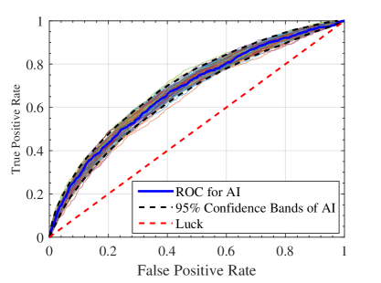
Figure 8: Bootstrapped ROC Curves for the Birth Defect Model.

Bold Blue line is for the original model, and other lines are bootstrapped ROC curves.

We then predict doctors’ diagnoses, where the labels in both the training data and the test data are the diagnosis by doctors, using the same deep learning algorithm as the one used to fit the observed birth defect outcome. The difference is that the dependent variable changes from birth defect outcomes to doctor’s diagnoses. Figure 9 shows the ROC curve of this algorithm with an AUC of 0.828. This procedure of training a model to predict the doctors’ diagnosis and using it to predict the same doctors’ diagnosis is different from the PROC curve discussed earlier where the model trained with the doctors’ diagnosis is used to predict the actual birth defect outcome. The AUC of 0.828 for this “predicted doctor’s model” is much higher than that for both the PROC and the MROC. It comes with no surprise that it is much easier to use features to predict the diagnosis by doctors, and to predict the actual outcome of birth defects.

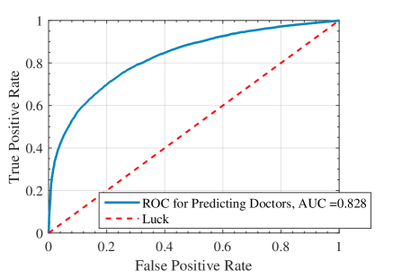
Figure 9: Empirical ROC curve for the model predicting doctor’s diagnoses

Figure 10 shows the MROC curve for the deep learning algorithm, the PROC curve for the predicted doctor’s model, and the FPR/TPR pair of average doctors. The AUC for MROC of the the deep learning algorithm is 0.677. The aggregate PTPR/PFPR pair of doctors lies significantly below the MROC. The PROC curve for predicted doctor’s model lies slightly above the aggregate doctors’ TPR/FPR, but below the machine learning ROC and has a lower AUC of about 0.533. Note that it is possible for the predicted humans’ model to outperform the humans TPR/FPR pair, as evident in Kleinberg et al. (2018). However, such an interpretation is subject to the concern due to Jensen’s inequality. Furthermore, the machine learning MROC and the “predicted doctor” PROC are two very different curves that encode different types of information and are not directly comparable.

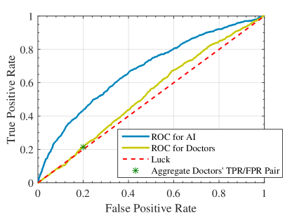
Figure 10: Empirical ROC curve for machine learning, predicted doctors model and real aggravated doctors

The $95\%$ confidence bands for the ROC curves of machines algorithm and predicted doctors are plotted via a bootstrap method. Since our sample size is large, the resulted bands are narrow. The AUCs of machine algorithm and predicted doctors are, respectively, $0.677\pm 0.012$ and $0.533\pm 0.024$ ($95\%$ confidence bands). Given that the AUC of machine algorithm is much larger than the predicted doctors, and both have small confidence bands. In the absence of incentive heterogeneity in decision making, the data provides strong statistical evidence in favor of the alternative hypothesis that the machine algorithm is better than the predicted doctor model in forecasting the actual birth defect outcomes.

If the doctors’ diagnosis (which is observed in the data) are only based on observed features $X$, it ought to be learned by the machine algorithm with a high level of precision. Consequently, the ROC for predicting doctors’ diagnosis should be very close to the $\left(0,1\right)$ vertex that represents perfect classification. However, as Figure 9 shows, the ROC for predicting doctors is still far away from perfect classification, in spite of the fact that doctors’ decisions are much easier to learn than the labeled actual outcomes. This is evident of the presence of incentive or informational heterogeneity in doctors’ diagnosis beyond those encoded in the observed features $X$.

6.3 Machines vs. Doctors

These findings from the data suggest provide potential evidence that both the machine learning algorithm and the “collective wisdom” of doctors outperform individual diagnosis, possibly because doctors misuse information. However, such interpretations need to be viewed with much caution, because essentially they are based on the assumptions that

1. Doctors used a homogeneous decision rule of the form of $\hat{Y}_{i}=\mathds{1}\left(\hat{q}\left(X_{i}\right)>c\right)$.

2. Doctors used the same or less information than the observed features $X$ to form an estimate of the propensity score $\hat{q}\left(X_{i}\right)$.

where $c$ is a constant cutoff point employed by all doctors. Both of these are strong assumptions that might be violated empirically. Possible alternative explanations of these empirical results may be caused by the heterogeneity of decision rules, which might include:

1. Heterogeneous incentives (various cutoff values across doctors).

2. Cutoff values depending on observed features for individual doctors.

We argue that incentive heterogeneity is likely to be present in an empirical data set. For example, using a million observation electronic birth data from New Jersey, Currie and MacLeod (2017) find strong evidence of heterogeneous decision making by doctors. Lembke (2012) suggests that online rating system tends to alter the incentive of practicing doctors. Some doctors care about online rating while some do not, creating incentive heterogeneity across doctors.

On the one hand, the MROC from machine learning represents information encoded in the observed features about the predictability of the outcome label. On the other hand, the aggregate TPR/FPR pair in the data encodes not only hetergeneous information dispersed among decision makers such as doctors, but also the heterogeneity in their incentives and preferences. Even if doctors know the true propensity score and therefore have as much information as the machine learning algorithm has, the aggregate PTPR/PFPR pair might still appear to be inferior as long as doctors employ a loss function that depends on the observed features. (Also refer to Section 5.2.1.) That the TPR/FPR pair lies below the MROC might be a mere reflection of preference heterogeneity among human decision makers instead of inferior information, and by itself does not provide evidence against the rationality and quality of human decision making.

6.4 Incentive Heterogeneity

We plotted the individual FPR and TPR pairs for those doctors who have diagnosed more than 100 patients in Figure 11. It is evident that doctors’ performance is highly heterogeneous. Some doctors are particularly conservative, showing high FPR and TPR. Although many doctors fall below the AI’s ROC curve, a fraction of the doctors show very high TPR and low FPR that lie above the machine learned ROC.

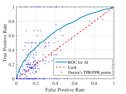
Figure 11: The heterogeneity of Doctors

For each doctor, we obtain the machine propensity score $p\left(x\right)$ from machine learning algorithm and doctors’ propensity score $q\left(x\right)$ from the predicted doctors’ model. We then run a regression using polynomial regressors up to the power of 5 to obtain the relationship between $p\left(x\right)$ and $q\left(x\right)$ (the $h$ function in section 5.2.2). To explicitly account for heterogeneity in decision making, we examine two doctors, one capable doctor with performance above the machine’s ROC curve and one incapable doctor with performance below the machine’s ROC curve. These two doctors see 1307 and 2254 patients, respectively, in our data set. Figure 12 and 13 show very different shapes for these two $h\left(x\right)$ functions, which is indicative of incentive heterogeneity among doctors.

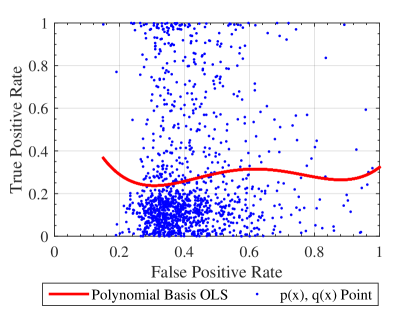
Figure 12: $p\left(x\right)$ vs. $q\left(x\right)$ for a capable doctor

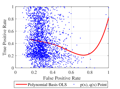
Figure 13: $p\left(x\right)$ vs. $q\left(x\right)$ for an incapable doctor

Furthermore, Figure 12 and 13 show that neither $h\left(x\right)$ function is monotonic, which implies the dependence of the cutoff threshold on observed features (refer to section 5.2.2). We also obtain the $h\left(x\right)$ function for all doctors, which is also a highly nonmonotonic function. For brevity, we hence omit the corresponding figure.

To control for incentive heterogeneity we make use of the conditioning idea in section 5.2.1 when we test the relative performance between humans and machines. We use the characteristic called “bad previous pregnancy outcomes” as the conditioning feature that the cutoff function depends on, where 0 stands for no bad previous outcomes and 1 for bad outcomes. We first remove the set of doctors whose TPR/FPR pairs under perform AI (see Figure 9). There are 3597 observations of class 0 and 490 observations of class 1 in the remaining data set. We use machine learning to make predictions for these two samples separately. The results are presented in the top two figures in Figure 14, where the doctors’ TPR/FPR pairs are on (slightly above) the corresponding AI’s ROC curves. Then, we use AI to predict the combined data set. This time, the doctors’ point falls below the AI’s ROC curve.

Figure 14: Empirical ROC curves and doctors’ performance conditional on the feature of "previous pregnancy outcomes"

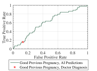
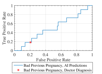
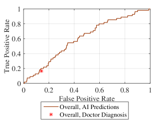
As discussed in Section 5.2.1, Figure 14 suggests that doctors’ cutoff thresholds depend on “bad previous pregnancy outcomes”. It also shows that even though doctors are better than AI, their aggregate TPR/FPR pair can be below AI’s ROC curve due to incentive heterogeneity with the dependence of cutoff points on features.

7 Conclusion

This paper studies the statistical properties of the Receiver Operating Characteristic (ROC) curve and its relation to binary classification and human decision making. We derive results that are useful for the construction of confidence bands for the ROC curve. We also show that a maximum AUC estimator is essentially the maximum score estimator from the econometrics literature, and discuss its implications for model selection and testing in binary classification problems. We use the Pre-Pregnancy Checkups of reproductive age couples in Henan Province provided by the Chinese Ministry of Health as an illustrative example for our theoretical model on ROC curves.

The advent of machine learning and artificial intelligence offers the potential of improving human decision making. A natural question to ask is whether machine learning can replace human decision makers. We conclude that the most commonly used performance measure, ROC curves, generated by a machine learning algorithm relative to a human decision maker does not translate into a statement about the superiority of the machine learning algorithm. We provide evidences in which human decision makers are fully rational yet appear to lie below the machine learned ROC curve. This is because ROC curve only provides a type of summary of information, yet decision making involves both information and incentives. These findings serve to clarify the misconception about ROC curves that appear in previous research papers.

8 Acknowledgements

We thank Xiaohong Chen, Andres Santos, and participants at various seminars and conferences for insightful comments. This study was approved by the National Health and Family Planning Commission. Informed consents were obtained from all the NFPC participants. We acknowledge funding support from the National Science Foundation (SES 1658950 to Han Hong), the National Science Fund for Distinguished Young Scholars of China (71325007 to Ke Tang), the State’s Key Project of Research and Development Plan (2016YFC1000307 to Jingyuan Wang) and the National Natural Science Foundation of China (61572059 to Jingyuan Wang).

Appendix A Appendix

Lemma A.1.

Denote $f_{p}\left(u\right)$ the implied density of the propensity score $p\left(x\right)$ induced by $f_{X}\left(x\right)$. Let $f_{p}\left(u\right)$ be positive and continuous on $u\in\left[0,1\right]$, then the ROC curve corresponding to a correctly specified $p\left(x\right)$ is a concave function.

Proof. We can write, where both size and power are now indexed by $c$:

$$\begin{split}\beta\left(c\right)=&\frac{1}{p}\int\mathds{1}\left(p\left(X\right)>c\right)p\left(X\right)f\left(X\right)\mathrm{d}X=\frac{1}{p}\int_{c}^{\infty}uf_{P}\left(u\right)\mathrm{d}u\end{split}$$

and

$$\begin{split}\alpha\left(c\right)=\frac{1}{1-p}\int\mathds{1}\left(p\left(X\right)>c\right)\left(1-p\left(X\right)\right)f\left(X\right)\mathrm{d}X=\frac{1}{1-p}\int_{c}^{\infty}\left(1-u\right)f_{p}\left(u\right)\mathrm{d}u.\end{split}$$

Hence

$$\begin{split}\frac{\mathrm{d}\beta}{\mathrm{d}c}=&-c\frac{f_{p}\left(c\right)}{p},\quad\frac{\mathrm{d}\alpha}{\mathrm{d}c}=-\left(1-c\right)\frac{f_{p}\left(c\right)}{1-p},\quad\frac{\mathrm{d}\beta}{\mathrm{d}\alpha}=\frac{c}{1-c},\end{split}$$

which is strictly increasing in $c$, and decreases when $c$ decreases from $1$ (at the origin of $\left(\alpha,\beta\right)=\left(0,0\right)$) to $0$ (at the $\left(\alpha,\beta\right)=(1,1)$ vertex).  

Lemma A.2.

In the absence of information heterogeneity, if the cutoff threshold $c$ varies among decision makers or within a single decision maker (incentive heterogeneity), the aggregate PTPR/PFPR pair of decision makers is below the optimal ROC curve.

Proof. To prove this, we write the pair as

$$\begin{split}\text{PFPR}=&\frac{1}{1-p}\int\lambda\left(x\right)\left(1-p\left(x\right)\right)f\left(x\right)\mathrm{d}x,\\ \text{PTPR}=&\frac{1}{p}\int\lambda\left(x\right)p\left(x\right)f\left(x\right)\mathrm{d}x,\end{split}$$

where $\lambda\left(x\right)=\int\mathds{1}\left(p\left(x\right)>h\left(x,v\right)\right)f\left(v\right)\mathrm{d}v$, note that the cutoff variable $h\left(x,v\right)$ depends on $x$ and a random variable $v$. We assume that the decision rule $\hat{Y}=\mathds{1}\left(p\left(x\right)>h\left(x,v\right)\right)$ has some classification ability, i.e. $\mathds{1}\left(p\left(x\right)>h\left(x,v\right)\right)\not\equiv 0$ and $\mathds{1}\left(p\left(x\right)>h\left(x,v\right)\right)\not\equiv 1$, therefore, $0<\lambda\left(x\right)<1$. Then for a $c^{*}$ satisfying

$$\alpha\left(c^{*}\right)= \int\mathds{1}\left(p\left(x\right)>c^{*}\right)\left(1-p\left(x\right)\right)f\left(x\right)\mathrm{d}x=\text{PFPR}=\int\lambda\left(x\right)\left(1-p\left(x\right)\right)f\left(x\right)\mathrm{d}x$$ (17)

on the optimal ROC curve, given the FPR $\alpha\left(c^{*}\right)$, we can find the TPR $\beta\left(c^{*}\right)$:

$$\beta\left(c^{*}\right)= \int\mathds{1}\left(p\left(x\right)>c^{*}\right)p\left(x\right)f\left(x\right)\mathrm{d}x.$$ (18)

Since $\alpha\left(c^{*}\right)$ and $\beta\left(c^{*}\right)$ are on the optimal ROC curve, by the Neyman-Pearson Lemma, there must be some positive $\eta_{1}$ and $\eta_{2}$ such that $\mathds{1}\left(p\left(x\right)>c^{*}\right)$ (but not $\lambda\left(x\right)$) solves

$$\arg\max_{\phi\left(\cdot\right)}\eta_{1}\int\phi\left(x\right)p\left(x\right)f\left(x\right)\mathrm{d}x-\eta_{2}\int\phi\left(x\right)\left(1-p\left(x\right)\right)f\left(x\right)\mathrm{d}x.$$ (19)

Hence $\eta_{1}\beta\left(c^{*}\right)-\eta_{2}\alpha\left(c^{*}\right)>\eta_{1}\text{PTPR}-\eta_{2}\text{PFPR}$, and thus $\beta\left(c^{*}\right)>\text{PTPR}$.  

Lemma A.3.

Let $p\left(X\right)$ and $q\left(X\right)$ be continuously distributed with a positive density on $\left[0,1\right]$, and $p\left(X\right)$ be correctly specified. These two propensity score functions $p\left(X\right)$ and $q\left(X\right)$ correspond to the same ROC if and if only if one is a strict monotonic transformation of the other.

Proof. The if part is immediate. Any point on the ROC of $p\left(X\right)$ maps into another point on th ROC of $q\left(X\right)$. Now consider the only if part. First we show that there exists a function $\bar{c}\left(t\right)$, such that for all $t$

$$\begin{split}\mathds{1}\left(q\left(X\right)\geq t\right)=\mathds{1}\left(p\left(X\right)\geq\bar{c}\left(t\right)\right)\end{split}$$

By assumption of the identical ROCs, $\bar{c}\left(t\right)$ exists such that,

$$\begin{split}\int\mathds{1}\left(q\left(x\right)\geq t\right)p\left(x\right)f\left(x\right)dx=&\int\mathds{1}\left(p\left(x\right)\geq\bar{c}\left(t\right)\right)p\left(x\right)f\left(x\right)dx,\\ \int\mathds{1}\left(q\left(x\right)\geq t\right)\left(1-p\left(x\right)\right)f\left(x\right)dx=&\int\mathds{1}\left(p\left(x\right)\geq\bar{c}\left(t\right)\right)\left(1-p\left(x\right)\right)f\left(x\right)dx.\end{split}$$

Note that the left hand sides are decreasing in $t$, and the right hand sides are decreasing in $\bar{c}\left(t\right)$, $\bar{c}\left(t\right)$ is necessarily an increasing function of $t$. To simplify, for $f\left(u,z\right)$ denoting the implied joint density of $\left(p\left(X\right),q\left(X\right)\right)$, we can write

$$\begin{split}\iint\mathds{1}\left(z\geq t\right)uf\left(u,z\right)\mathrm{d}u\mathrm{d}z=&\iint\mathds{1}\left(u\geq\bar{c}\left(t\right)\right)uf\left(u,z\right)\mathrm{d}u\\ \iint\mathds{1}\left(z\geq t\right)f\left(u,z\right)\mathrm{d}u\mathrm{d}z=&\iint\mathds{1}\left(u\geq\bar{c}\left(t\right)\right)f\left(u,z\right)\mathrm{d}u\mathrm{d}z\end{split}$$

which can be written as

$$\begin{split}\int\mathbb{E}\left[\mathds{1}\left(z\geq t\right)|u\right]uf\left(u\right)\mathrm{d}u=&\int\mathds{1}\left(u\geq\bar{c}\left(t\right)\right)uf\left(u\right)\mathrm{d}u\\ \int\mathbb{E}\left[\mathds{1}\left(z\geq t\right)|u\right]\left(1-u\right)f\left(u\right)\mathrm{d}u=&\int\mathds{1}\left(u\geq\bar{c}\left(t\right)\right)\left(1-u\right)f\left(u\right)\mathrm{d}u.\end{split}$$ (20)

By Neyman-Pearson Lemma’s argument,

$$\begin{split}\mathbb{E}\left[\mathds{1}\left(z\geq t\right)|u\right]=\mathds{1}\left(u\geq\bar{c}\left(t\right)\right)\end{split}$$ (21)

which implies that $\mathds{1}\left(z\geq t\right)=\mathds{1}\left(u\geq\bar{c}\left(t\right)\right)$. To see (21), let $h\left(u,t\right)\equiv\mathbb{E}\left[\mathds{1}\left(z\geq t\right)|u\right]$. Take a linear combination of the two equalities in (20) using $\left(1-\bar{c}\left(t\right)\right)$ and $-\bar{c}\left(t\right)$,

$$\begin{split}\int h\left(u,t\right)\left[\left(1-\bar{c}\left(t\right)\right)u-\bar{c}\left(t\right)\left(1-u\right)\right]f\left(u\right)du.\end{split}$$

The function $h\left(u,t\right)$ that maximizes the above integral is obviously $h\left(u,t\right)=1\left(u\geq c\left(t\right)\right)$, which appears on the right hand sides of (20). Therefore in order for both inequalities in (20) to hold, it must be the case that $h\left(u,t\right)\equiv\mathbb{E}\left[\mathds{1}\left(z\geq t\right)|u\right]=1\left(u\geq c\left(t\right)\right)$.

Next we verify again that $\bar{c}\left(t\right)$ is strictly monotonic. Define $X_{p}\left(c\right)=\{x:p\left(x\right)\geq c\}$, and $X_{q}\left(t\right)=\{x:q\left(x\right)\geq t\}$. By definition,

$$\begin{split}X_{p}\left(c_{2}\right)\subset X_{p}\left(c_{1}\right)\quad\text{iff}\quad c_{1}<c_{2},\quad X_{q}\left(t_{2}\right)\subset X_{q}\left(t_{1}\right)\quad\text{iff}\quad t_{1}<t_{2}.\end{split}$$

Then for $X_{q}\left(t\right)=X_{p}\left(\bar{c}\left(t\right)\right)$, it must be that $\bar{c}\left(t_{1}\right)>\bar{c}\left(t_{2}\right)$ if $t_{1}>t_{2}$. Then an inverse function $\bar{c}^{-1}\left(\cdot\right)$ exists, and for all $t$,

$$\begin{split}X_{q}\left(t\right)=X_{p}\left(\bar{c}\left(t\right)\right)=\{x:\bar{c}^{-1}\left(p\left(x\right)\right)\geq t\}.\end{split}$$

So that $q\left(x\right)=\bar{c}^{-1}\left(p\left(x\right)\right)$.  

Lemma A.4.

In the absence of information and incentive heterogeneity beyond the observed features, the predicted doctor ROC degenerates to a singleton.

Proof. To see this, the predicted human is a step function that takes only values $0$ and $1$: if $D=1\left(\bar{p}\left(X\right)\geq c_{0}\right)$, then

$$\begin{split}q\left(X\right)\equiv\mathbb{P}\left(D=1|X\right)=\mathbb{P}\left(\bar{p}\left(X\right)>c_{0}|X\right)=\mathds{1}\left(\bar{p}\left(X\right)>c_{0}\right),\end{split}$$

The resulting ROC curve for the predicted human is given by

$$\begin{split}\bar{\beta}\left(c\right)=&\frac{1}{p}\int\mathds{1}\left(1\left(\bar{p}\left(x\right)>c_{0}\right)>c\right)p\left(x\right)f\left(x\right)\mathrm{d}x\\ \bar{\alpha}\left(c\right)=&\frac{1}{1-p}\int\mathds{1}\left(1\left(\bar{p}\left(x\right)>c_{0}\right)>c\right)\left(1-p\left(x\right)\right)f\left(x\right)\mathrm{d}x.\end{split}$$

Note that

$$\begin{split}\bar{\beta}\left(c\right)=&\frac{1}{p}\int\mathds{1}\left(\bar{p}\left(x\right)>c_{0}\right)p\left(x\right)f\left(x\right)\mathrm{d}x,\\ \bar{\alpha}\left(c\right)=&\frac{1}{1-p}\int\mathds{1}\left(\bar{p}\left(x\right)>c_{0}\right)\left(1-p\left(x\right)\right)f\left(x\right)\mathrm{d}x.\end{split}$$

which does not even depend on $c$. Therefore the ROC of the predicted doctor should be a singleton point.  

Lemma A.5.

If humans make correct use of additional information $U$ beyond the observed features $X$, and predicted humans’ ROC lies above the machine learned ROC.

Proof. For a formal proof, note that the ROC curve is defined by the locus of the pair of functions $\left(\alpha\left(c\right),\beta\left(c\right),c\in\left(0,1\right)\right),$ where

$$\begin{split}\alpha\left(c\right)=&\frac{1}{1-p}\iint\mathds{1}\left(p\left(x,u\right)>c\right)\left(1-p\left(x,u\right)\right)f\left(x,u\right)\mathrm{d}x\mathrm{d}u\\ \beta\left(c\right)=&\frac{1}{p}\iint\mathds{1}\left(p\left(x,u\right)>c\right)p\left(x,u\right)f\left(x,u\right)\mathrm{d}x\mathrm{d}u.\end{split}$$

By definition and by Neyman-Pearson arguments, it must lie above the ROC curve defined by the locus of $\left(\bar{\alpha}\left(c\right),\bar{\beta}\left(c\right),c\in\left(0,1\right)\right)$, where

$$\begin{split}\bar{\alpha}\left(c\right)=&\frac{1}{1-p}\iint\mathds{1}\left(p\left(x\right)>c\right)\left(1-p\left(x,u\right)\right)f\left(x,u\right)\mathrm{d}x\mathrm{d}u\\ \bar{\beta}\left(c\right)=&\frac{1}{p}\iint\mathds{1}\left(p\left(x\right)>c\right)p\left(x,u\right)f\left(x,u\right)\mathrm{d}x\mathrm{d}u.\end{split}$$

But

$$\begin{split}\bar{\beta}\left(c\right)=\frac{1}{p}\int\mathds{1}\left(p\left(x\right)>c\right)\int p\left(x,u\right)f\left(u|x\right)\mathrm{d}uf\left(x\right)\mathrm{d}x=\frac{1}{p}\int\mathds{1}\left(p\left(x\right)>c\right)p\left(x\right)f\left(x\right)\mathrm{d}x,\end{split}$$

and similarly,

$$\begin{split}\bar{\alpha}\left(c\right)=&\frac{1}{1-p}\int\mathds{1}\left(p\left(x\right)>c\right)\int\left(1-p\left(x,u\right)\right)f\left(u|x\right)\mathrm{d}uf\left(x\right)\mathrm{d}x\\ =&\frac{1}{p}\int\mathds{1}\left(p\left(x\right)>c\right)\left(1-p\left(x\right)\right)f\left(x\right)\mathrm{d}x,\end{split}$$

Consequently, $\bar{\alpha}\left(c\right),\bar{\beta}\left(c\right),c\in\left(0,1\right)$ is also the ROC curve defined by $p\left(X\right)$.

Therefore, for the case of homogeneous preference but heterogeneity in information, if the information is correct, the aggregate PTPR/PFPR pair must lie above the machine optimal ROC.  

Generalization of Sherman (1993) under misspecification

Without the single index assumption, suitable location and scale normalization, including removing the constant term in $X_{i}$ and fixing the first element of $\theta$ at $1$ as in as in Sherman (1993), is still necessary for identification. Here we describe the generalization of section 6 in Sherman (1993) to allow for misspecification of the single index model.

Recall the kernel function for the U-statistics on pp 129 Sherman (1993), for $Z=\left(Y,X\right)$,

$$\begin{split}\tau\left(z,\theta\right)=&\mathbb{E}\left[\mathds{1}\left(x^{\prime}\beta\left(\theta\right)>X^{\prime}\beta\left(\theta\right)\right)\mathds{1}\left(y>Y\right)+\mathds{1}\left(x^{\prime}\beta\left(\theta\right)<X^{\prime}\theta\right)\mathds{1}\left(y<Y\right)\right]\\ =&\mathbb{E}\left[\mathds{1}\left(x^{\prime}\beta\left(\theta\right)>X_{j}^{\prime}\beta\left(\theta\right)\right)\left(\mathds{1}\left(y>Y_{j}\right)-\mathds{1}\left(y<Y_{j}\right)\right)\right]+\mathbb{E}\left[\mathds{1}\left(y<Y_{j}\right)\right]\end{split}$$

Without requiring the single index model, Theorem 4 of Sherman (1993) shows that

$$\begin{split}\sqrt{n}\left(\hat{\theta}-\theta^{*}\right)=\frac{1}{\sqrt{n}}\sum_{i=1}^{n}\kappa_{i}+o_{P}\left(\frac{1}{\sqrt{n}}\right),\quad\kappa_{i}=V^{-1}\frac{\partial}{\partial\theta}\tau\left(Z_{i},\theta\right),\quad 2V=\frac{\partial^{2}}{\partial\theta\partial\theta^{\prime}}E\tau\left(Z_{i},\theta\right).\end{split}$$

The influence function can be computed without referencing the single index assumption and through the use of a Dirac function $\delta_{0}\left(\cdot\right)$,

$$\begin{split}\frac{\partial}{\partial\theta}\tau\left(Z_{i},\theta\right)=&\frac{\partial}{\partial\theta}\iint\mathds{1}\left(\left(X_{i}-w\right)^{\prime}\beta\left(\theta\right)>0\right)\left(\mathds{1}\left(Y_{i}>z\right)-\mathds{1}\left(Y_{i}<z\right)\right)f_{Y,X}\left(z,w\right)\mathrm{d}w\mathrm{d}z\\ =&\int\left(\bar{X}_{i}-\bar{w}\right)\delta_{0}\left(\left(X_{i}-w\right)^{\prime}\beta\left(\theta\right)\right)S\left(Y_{i},w\right)f_{X}\left(w\right)\mathrm{d}w\end{split}$$

where $\bar{X}_{i}$ and $\bar{w}$ denote the corresponding vectors without the first element,

$$\begin{split}S\left(Y_{i},w\right)=\int\left(\mathds{1}\left(Y_{i}>z\right)-\mathds{1}\left(Y_{i}<z\right)\right)f_{Y|X}\left(z|w\right)\mathrm{d}z=2F_{Y|X}\left(Y_{i}|w\right)-1.\end{split}$$

Consider the transformation $w\Longrightarrow\left(t=w^{\prime}\beta\left(\theta\right)=w_{1}+\bar{w}^{\prime}\theta,\bar{w}\right)$, with the inverse transformation $\left(t,\bar{w}\right)\Longrightarrow\left(t-\theta^{\prime}\bar{w},\bar{w}\right)$. Note that the determinant of this transform is $1$. Then we can apply this transformation to write

$$\begin{split}\frac{\partial}{\partial\theta}\tau\left(Z_{i},\theta\right)=&\iint\left(\bar{X}_{i}-\bar{w}\right)\delta_{0}\left(t-X_{i}^{\prime}\beta\left(\theta\right)\right)S\left(Y_{i},\left(t-\bar{w}^{\prime}\theta,\bar{w}\right)\right)f_{X}\left(\bar{w},t\right)\mathrm{d}\bar{w}\mathrm{d}t\\ =&\int\left(\bar{X}_{i}-\bar{w}\right)S\left(Y_{i},\left(X_{i}^{\prime}\beta\left(\theta\right)-\bar{w}^{\prime}\theta,\bar{w}\right)\right)f_{X}\left(\bar{w},X_{i}^{\prime}\beta\left(\theta\right)\right)\mathrm{d}\bar{w}\end{split}$$

Further “simplication” beyond this point does not appear to be feasible without the single index and correct specification conditions in Sherman (1993). Yet the above influence function is still valid for asymptotic inference. The Hessian term can be computed by further differentiation,

$$\begin{split}2V=\iint\frac{\partial}{\partial\theta}\frac{\partial}{\partial\theta}\tau\left(z,\theta\right)f_{Y,X}\left(y,x\right)\mathrm{d}y\mathrm{d}x\end{split}$$

which in general will involve both $\frac{\partial}{\partial\theta}S\left(Y_{i},\left(t-\bar{w}^{\prime}\theta,\bar{w}\right)\right)$ and $\frac{\partial}{\partial\theta}f_{X}\left(\bar{w},X_{i}^{\prime}\beta\left(\theta\right)\right)$.

Similar to Sherman (1993), numerical differentiation can be employed to consistently estimate the influence function (hence its asymptotic variance as well), and the limiting Hessian, using step sizes that satisfy $\sqrt{n}\epsilon_{n}\rightarrow\infty$ and $n^{1/4}\epsilon_{n}\rightarrow\infty$, respectively. The arguments for the consistency of numerical derivatives in Sherman (1993) do not depend on a correct specified single index model either, and only depend on the Euclidean properties of a monotone transformation of the linear index function. See also Hong et al. (2015).

References

- (1)
- Bamber (1975) Bamber, Donald, “The area above the ordinal dominance graph and the area below the receiver operating characteristic graph,” Journal of Mathematical Psychology, 1975, 12 (4), 387–415.
- Chandra and Staiger (2011) Chandra, Amitabh and Douglas O Staiger, “Expertise, underuse, and overuse in healthcare,” Working Paper, 2011.
- Currie and MacLeod (2017) Currie, Janet and W Bentley MacLeod, “Diagnosing expertise: Human capital, decision making, and performance among physicians,” Journal of Labor Economics, 2017, 35 (1), 1–43.
- Elliott and Lieli (2013) Elliott, Graham and Robert P Lieli, “Predicting binary outcomes,” Journal of Econometrics, 2013, 174 (1), 15–26.
- Esteva et al. (2017) Esteva, Andre, Brett Kuprel, Roberto A Novoa, Justin Ko, Susan M Swetter, Helen M Blau, and Sebastian Thrun, “Dermatologist-level classification of skin cancer with deep neural networks,” Nature, 2017, 542 (7639), 115.
- Fawcett (2006) Fawcett, Tom, “An introduction to ROC analysis,” Pattern Recognition Letters, 2006, 27 (8), 861–874.
- Fisher (1936) Fisher, Ronald A, “The use of multiple measurements in taxonomic problems,” Annals of Human Genetics, 1936, 7 (2), 179–188.
- Glorot and Bengio (2010) Glorot, Xavier and Yoshua Bengio, “Understanding the difficulty of training deep feedforward neural networks,” Journal of Machine Learning Research, 2010.
- Gulshan et al. (2016) Gulshan, Varun, Lily Peng, Marc Coram, Martin C Stumpe, Derek Wu, Arunachalam Narayanaswamy, Subhashini Venugopalan, Kasumi Widner, Tom Madams, Jorge Cuadros et al., “Development and validation of a deep learning algorithm for detection of diabetic retinopathy in retinal fundus photographs,” JAMA, 2016, 316 (22), 2402–2410.
- Guo and Berkhahn (2016) Guo, Cheng and Felix Berkhahn, “Entity embeddings of categorical variables,” arXiv preprint arXiv:1604.06737, 2016.
- Hand and Till (2001) Hand, David J and Robert J Till, “A simple generalisation of the area under the ROC curve for multiple class classification problems,” Machine Learning, 2001, 45 (2), 171–186.
- Hanley and McNeil (1982) Hanley, James A and Barbara J McNeil, “The meaning and use of the area under a receiver operating characteristic (ROC) curve.,” Radiology, 1982, 143 (1), 29–36.
- Hoeffding et al. (1948) Hoeffding, Wassily et al., “A class of statistics with asymptotically normal distribution,” The Annals of Mathematical Statistics, 1948, 19 (3), 293–325.
- Hong et al. (2015) Hong, Han, Aprajit Mahajan, and Denis Nekipelov, “Extremum estimation and numerical derivatives,” Journal of Econometrics, 2015, 188 (1), 250–263.
- Hong et al. (2003) , Bruce Preston, and Matthew Shum, “Generalized empirical likelihood–based model selection criteria for moment condition models,” Econometric Theory, 2003, 19 (6), 923–943.
- Hsieh et al. (1996) Hsieh, Fushing, Bruce W Turnbull et al., “Nonparametric and semiparametric estimation of the receiver operating characteristic curve,” The Annals of Statistics, 1996, 24 (1), 25–40.
- Huang and Ling (2005) Huang, Jin and Charles X Ling, “Using AUC and accuracy in evaluating learning algorithms,” IEEE Transactions on Knowledge and Data Engineering, 2005, 17 (3), 299–310.
- Ioffe and Szegedy (2015) Ioffe, Sergey and Christian Szegedy, “Batch normalization: accelerating deep network training by reducing internal covariate shift,” International Conference on Machine Learning, 2015, pp. 448–456.
- Kermany et al. (2018) Kermany, Daniel S, Michael Goldbaum, Wenjia Cai, Carolina CS Valentim, Huiying Liang, Sally L Baxter, Alex McKeown, Ge Yang, Xiaokang Wu, Fangbing Yan et al., “Identifying medical diagnoses and treatable diseases by image-based deep learning,” Cell, 2018, 172 (5), 1122–1131.
- Kleinberg et al. (2018) Kleinberg, Jon, Himabindu Lakkaraju, Jure Leskovec, Jens Ludwig, and Sendhil Mullainathan, “Human Decisions and Machine Predictions,” The Quarterly Journal of Economics, 2018, 133 (1), 237–293.
- Kosorok (2007) Kosorok, Michael R, Introduction to empirical processes and semiparametric inference., Springer, 2007.
- Lehmann (2004) Lehmann, Erich Leo, Elements of large-sample theory, Springer Science & Business Media, 2004.
- Lembke (2012) Lembke, Anna, “Why doctors prescribe opioids to known opioid abusers,” New England Journal of Medicine, 2012, 367 (17), 1580–1581.
- Long et al. (2017) Long, Erping, Haotian Lin, Zhenzhen Liu, Xiaohang Wu, Liming Wang, Jiewei Jiang, Yingying An, Zhuoling Lin, Xiaoyan Li, Jingjing Chen et al., “An artificial intelligence platform for the multihospital collaborative management of congenital cataracts,” Nature Biomedical Engineering, 2017, 1 (2), 0024.
- Newey and McFadden (1994) Newey, Whitney K and Daniel McFadden, “Large sample estimation and hypothesis testing,” Handbook of Econometrics, 1994, 4, 2111–2245.
- Rajpurkar et al. (2017) Rajpurkar, Pranav, Awni Y Hannun, Masoumeh Haghpanahi, Codie Bourn, and Andrew Y Ng, “Cardiologist-level arrhythmia detection with convolutional neural networks,” arXiv preprint arXiv:1707.01836, 2017.
- Sherman (1993) Sherman, Robert P, “The limiting distribution of the maximum rank correlation estimator,” Econometrica: Journal of the Econometric Society, 1993, pp. 123–137.
- Srivastava et al. (2014) Srivastava, Nitish, Geoffrey E Hinton, Alex Krizhevsky, Ilya Sutskever, and Ruslan Salakhutdinov, “Dropout: a simple way to prevent neural networks from overfitting,” Journal of Machine Learning Research, 2014, 15 (1), 1929–1958.
- Vuong (1989) Vuong, Quang H, “Likelihood ratio tests for model selection and non-nested hypotheses,” Econometrica: Journal of the Econometric Society, 1989, pp. 307–333.
- Yang et al. (2015) Yang, Bishan, Wentau Yih, Xiaodong He, Jianfeng Gao, and Li Deng, “Embedding entities and relations for learning and inference in knowledge Bases,” International Conference on Learning Representations, 2015.