Carbon radio recombination lines from gigahertz to megahertz frequencies towards Orion A

Abstract

Context. The combined use of carbon radio recombination lines (CRRLs) and the $158$ $\mu$m-[CII] line is a powerful tool for the study of the energetics and physical conditions (e.g., temperature and density) of photodissociation regions (PDRs). However, there are few observational studies that exploit this synergy.

Aims. Here we explore the relation between CRRLs and the $158$ $\mu$m-[CII] line in light of new observations and models.

Methods. We present new and existing observations of CRRLs in the frequency range $0.15$–$230$ GHz with ALMA, VLA, the GBT, Effelsberg 100m, and LOFAR towards Orion A (M42). We complement these observations with SOFIA observations of the $158$ $\mu$m-[CII] line. We studied two PDRs: the foreground atomic gas, known as the Veil, and the dense PDR between the HII region and the background molecular cloud.

Results. In the Veil we are able to determine the gas temperature and electron density, which we use to measure the ionization parameter and the photoelectric heating efficiency. In the dense PDR, we are able to identify a layered PDR structure at the surface of the molecular cloud to the south of the Trapezium cluster. There we find that the radio lines trace the colder portion of the ionized carbon layer, the C⁺/C/CO interface. By modeling the emission of the $158$ $\mu$m-[CII] line and CRRLs as arising from a PDR we derive a thermal pressure $>5\times 10^{7}$ K cm^-3 and a radiation field $G_{0}\approx 10^{5}$ close to the Trapezium.

Conclusions. This work provides additional observational support for the use of CRRLs and the $158$ $\mu$m-[CII] line as complementary tools to study dense and diffuse PDRs, and highlights the usefulness of CRRLs as probes of the C⁺/C/CO interface.

1 Introduction

The transfer of material from the massive reservoirs of the cold neutral medium (CNM, $T\sim 80$ K) into cold molecular clouds partially regulates the star formation cycle in a galaxy (e.g., Klessen & Glover 2016). This conversion of atomic to molecular gas is intimately related to the heating and cooling processes the gas experiences.

The heating and cooling of atomic gas can be studied in photodissociation regions (PDRs; e.g., Hollenbach & Tielens 1999). These are regions where the influence of far-ultraviolet (FUV) photons shape the interstellar medium (ISM) into a layered structure with hydrogen ionized or neutral close to the source of radiation and molecular farther from it. PDRs can be found in dense and in diffuse regions; the former happen close to sites of star formation where the FUV radiation from young stars impinges on the surface of their natal molecular cloud, while the latter can be found throughout most of the CNM, powered by the interstellar radiation field (ISRF).

For the CNM and in PDRs, one of the main cooling mechanisms is through the far-infrared (FIR) fine-structure line of ionized carbon ([CII]) at $158$ $\mu$m (e.g., Field et al. 1969; Dalgarno & McCray 1972; Pottasch et al. 1979; Wolfire et al. 1995, 2003). Since carbon has a lower ionization potential than hydrogen, it is ionized throughout the diffuse ISM and in PDR surfaces, and with an energy difference between its fine structure states of $91.2$ K, it is easily excited. However, this implies that the $158$ $\mu$m-[CII] line will also trace other phases of the ISM. These phases include the warm ionized medium (WIM, $T\sim 8000$ K), extended low density WIM (ELDWIM; e.g., Heiles 1994), extended low density HII regions (e.g., Goldsmith et al. 2015), and also the surfaces of molecular clouds (e.g., Visser et al. 2009; Wolfire et al. 2010). It has been estimated that $\sim 21\%$ of the $158$ $\mu$m-[CII] line in our Galaxy is produced in the CNM and $\sim 47\%$ in dense PDRs (Pineda et al. 2013). In order to measure the cooling rate of the CNM, we must be able to isolate its contribution to the excitation of the $158$ $\mu$m-[CII] line (e.g., Pabst et al. 2017).

The separation between cold and warm gas can be done using carbon radio recombination lines (CRRLs e.g., Gordon & Sorochenko 2009). These are lines produced when a carbon ion recombines with an electron to a large principal quantum number $n$ resulting in a Rydberg atom. When a Rydberg atom of carbon transitions between different principal quantum numbers it will produce CRRLs, from gigahertz to megahertz frequencies depending on the $n$ levels involved. The optical depth of the produced CRRL has a strong dependence on the gas temperature ($\tau\propto T^{-5/2}$), so CRRLs have little contamination from warm gas or HII regions. Thus, we can use CRRLs to isolate emission from the CNM and the surfaces of molecular clouds and their contribution to the $158$ $\mu$m-[CII] line excitation.

Another property of CRRLs is that the population of carbon atoms in each energy state is determined by the gas density, temperature, and radiation field, as well as the atomic physics involved (e.g., Shaver 1975; Watson et al. 1980; Salgado et al. 2017a). Therefore, it is possible to determine the gas physical conditions by observing CRRLs at a range of frequencies and comparing this to the predicted line properties (e.g., Dupree 1974; Payne et al. 1989; Roshi & Kantharia 2011; Salgado et al. 2017b; Oonk et al. 2017; Salas et al. 2018).

Moreover, given that CRRLs have a different temperature dependency from the $158$ $\mu$m-[CII] line, we can combine both types of lines to determine the gas temperature and/or density (e.g., Natta et al. 1994; Smirnov et al. 1995; Salgado et al. 2017b; Salas et al. 2017). This approach is particularly useful as it requires observations of a few of the faint CRRLs ($\tau\sim 10^{-3}$–$10^{-4}$) instead of a large set of them to reach a similar accuracy on the derived gas properties. However, the combined use of the $158$ $\mu$m-[CII] line and CRRLs has been performed only towards a handful of sources and using observations which do not resolve the lines in velocity and/or do not have the same angular resolution.

One of the sources that has been studied in CRRLs and in the $158$ $\mu$m-[CII] line is the Orion star forming region. Orion A is a nearby giant molecular cloud that covers $\approx 29$ deg² (Maddalena et al. 1986). In the northern part of this cloud we can find the Orion nebula cluster (ONC; e.g., Pickering 1917; Sharpless 1952; O’Dell 2001), the region of massive star formation that is closest to Earth. The brightest stars in the ONC are the Trapezium stars (M42, $(\alpha,\delta)_{\mathrm{J2000}}=(5^{\mathrm{h}}35^{\mathrm{m}}17.3^{\mathrm{s}},-5^{\circ}23^{\mathrm{m}}28^{\mathrm{s}})$, e.g., Large et al. 1981). The ionizing radiation from the Trapezium stars has created a HII region. M42 lies in front of Orion A, which makes it easier for the ionizing radiation to escape towards the observer (Zuckerman 1973; Balick et al. 1974a, b). Behind the Trapezium stars and the HII region, Orion A is arranged in an S-shaped structure known as the integral shaped filament (ISF, Bally et al. 1987). In front of the Trapezium stars and the HII region, there are layers of neutral gas collectively known as the Veil (e.g., van der Werf & Goss 1989; Abel et al. 2004; O’Dell et al. 2009; van der Werf et al. 2013; Troland et al. 2016). Observations of the $21$ cm-HI line at high spatial resolution ($\approx 7\arcsec$) show that the gas in the Veil is composed of two spatially distinct velocity components: component A at $5.3$ km s^-1 and component B at $1.3$ km s^-1 (van der Werf & Goss 1989). The proximity and geometry of M42, sandwiched between a high density molecular cloud and the diffuse gas in the Veil, makes it an ideal target to study how the gas cooling rate changes between dense and diffuse gas.

The goal of this work is to re-evaluate the relation between the $158$ $\mu$m-[CII] line and CRRLs at radio frequencies in the light of new models and observations of Orion A. We take advantage of new large-scale maps ($\approx 1$ deg²) of the $158$ $\mu$m-[CII] line in the FIR (Pabst et al. 2019). This improves on previous comparisons that used velocity unresolved observations of the $158$ $\mu$m-[CII] line (Natta et al. 1994). The velocity resolution of the $158$ $\mu$m-[CII] line observations in this study was of $\approx 50$ km s^-1, while in the observations of Pabst et al. (2019) this is $0.2$ km s^-1. Additionally, we use models that describe the level population of carbon atoms including the effect of dielectronic capture (Salgado et al. 2017a). Incorporating this effect can change the predicted CRRL intensities by a factor of two (e.g., Wyrowski et al. 1997).

This work is organized as follows. In Section 2 we start by presenting the observations used. We present the results obtained from these observations in Section 3. In Section 4 we derive physical conditions from our results; these conditions are also compared against results found in the literature. We conclude with a summary of our work in Section 5.

In this work, all velocities are given in the local standard of rest unless otherwise specified. To convert to heliocentric velocities $18.1$ km s^-1 should be added. We adopt a distance of $414$ pc to Orion A (e.g., Menten et al. 2007; Zari et al. 2017).

2 Observations and data reduction

We start by describing previously unpublished CRRL observations. They include an L-band ($1$ GHz to $2$ GHz) map of CRRLs; pointings towards M42, which include CRRLs at frequencies between $2.8$ GHz and $275$ MHz; and a cube of CRRL absorption at $150$ MHz. We also briefly describe CRRL observations taken from the literature, as well as observations of other tracers relevant for this work.

2.1 GBT observations

2.1.1 L-band CRRL maps

We observed Orion A with the National Radio Astronomy Observatory (NRAO) Robert C. Byrd Green Bank Telescope (GBT) during seven nights in November $2016$ (project: AGBT16B_225). We mapped a $\approx 0.4\degr\times 1\degr$ region centered on $(\alpha,\delta)_{\mathrm{J2000}}=5^{\mathrm{h}}35^{\mathrm{m}}14.5^{\mathrm{s}},-5\degr 22^{\mathrm{m}}29.3^{\mathrm{s}}$ using the on-the-fly imaging technique (e.g., Mangum et al. 2007). The observations were performed using the L-band ($1.1$–$1.8$ GHz) receiver and the Versatile GBT Astronomical Spectrometer (VEGAS; Bussa & VEGAS Development Team 2012). VEGAS was set up to process $27$ spectral windows $23.44$ MHz wide. Each spectral window was split into $65536$ channels of $0.357$ kHz in width. The spectral windows were centered on the $21$ cm-HI line, the four $18$ cm-OH lines, and the remaining on RRLs within the GBT L-band range. As an absolute flux calibrator we observed 3C123 (Baars et al. 1977) with the Perley & Butler (2013) flux scale to convert from raw counts to temperature. We adopted the methods described in Winkel et al. (2012) to convert the raw units to temperature when possible. As is discussed below, in some steps this was not possible due to the high continuum brightness of Orion A. A summary of the observational setup is presented in Table 2.

Table 1: GBT mapping observation parameters

Project code	AGBT16B_225
Observation dates	5, 6, 8, 9, 10, 15 and
	17 of November 2016
	and 2 of December 2016.
Polarizations	XX,YY
Spectral windows	27
Spectral window frequencies (MHz)	1156, 1176, 1196,
	1217, 1240, 1259,
	1281, 1304, 1327,
	1351, 1375, 1400,
	1420.4, 1425, 1451,
	1478, 1505, 1533,
	1561, 1591, 1608,
	1621, 1652, 1665.4,
	1684, 1716, 1720.53
Spectral window	23.44
bandwidth (MHz)
Channels per spectral window	65536
Integration time	10.57
per spectral dump (s)
Absolute flux calibrator	3C123
Total observing time	$15$ hours
Principal quantum numbers	$156$–$178$

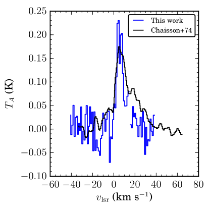
Figure 1: Comparison between the temperature-calibrated GBT C$157\alpha$ line and the C$158\alpha$ observation of Chaisson (1974). The temperature scales of the two spectra agree over the brightest portion of M42, the most affected by a nonlinearity in the signal path (see text for details). Both spectra were extracted from an aperture of diameter $18\arcmin$ centered on $(\alpha,\delta)_{\mathrm{J2000}}=(5^{\mbox{h}}35^{\mbox{m}}17.45^{\mbox{s}},-5\degr 23^{\mbox{m}}46.8^{\mbox{s}})$. The on-source time of the C$157\alpha$ observations is roughly seven minutes, while that of the C$158\alpha$ observations is $1200$ minutes. The resolution of the C$158\alpha$ spectrum is $1.9$ km s^-1 (Chaisson 1974) and that of the C$157\alpha$ spectrum is $1$ km s^-1.

The mapped region was subdivided into smaller maps in order to keep the variations in antenna temperature within the three dB dynamical range of VEGAS. At the beginning of each session, the pointing and focus solutions were updated on 3C161. The pointing corrections were less than $10\%$ of the beam width.

Given the high continuum brightness of Orion A ($\sim 375$ Jy or $600$ K at $1.4$ GHz, e.g., Goudis 1975), the telescope amplifiers were saturated over the brightest portions of the source. The saturation produced a compression of the amplifier gain. In order to correct for the nonlinearity in the conversion from raw counts to brightness temperature in the affected portions of the map, we followed a procedure similar to that used by the GBT intermediate frequency nonlinearity project and briefly outlined in Appendix A. To quantitatively determine the deviation from a linear gain we compared the raw counts against the $21$ cm continuum maps of van der Werf et al. (2013). To scale the temperature of the van der Werf et al. (2013) map across the $700$ MHz wide frequency range used in the GBT observations we use the results of Lockman & Brown (1975). Lockman & Brown (1975) present a compilation of continuum measurements of Orion A. According to these measurements, the brightness temperature of the source scales as $T_{\mathrm{M42}}\propto\nu^{-1.7}$ between $1.1$ GHz and $1.8$ GHz. After converting the data to temperature units we compared the resulting spectra against previously published values. An example of this comparison is shown in Figure 1, where we compare the C$158\alpha$ spectrum against that observed by Chaisson (1974) using the $42.7$ m antenna of the NRAO. The uncertainty on the absolute flux calibration is $\approx 20\%$, considering the nonlinear gain correction.

Before gridding all maps together, we checked that the line profiles on overlapping regions agreed. We found no significant differences among the maps. Then all the data was gridded together using the stand-alone GBTGRIDDER. With this program we produced a CRRL cube for each line observed.

To obtain the best spatial resolution possible from these observations, we stacked the first three CRRLs observed ($156$, $157$, and $158$) in one cube. This produced a cube with a half power beam width (HPBW) of $\approx 8\aas@@fstack{\prime}1$ and an average principal quantum number of $157$. To increase the signal-to-noise ratio of the cube, we averaged in velocity to a channel width of $\approx 1$ km s^-1 (Figure 1).

2.1.2 Pointings towards M42

We searched the NRAO archive for observations of M42. From the available observations we used projects AGBT02A_028, AGBT12A_484, and AGBT14B_233. They correspond to single pointings of M42 with the GBT that have a spectral resolution adequate for spectral line analysis ($\approx 1$ km s^-1 spectral resolution). A summary of these observations is provided in Table 5.

Table 2: GBT single-pointing observation parameters

Project code	Frequency ranges	Aperture efficiency	HPBW	Principal quantum
	(MHz)		($\arcmin$)	numbers
AGBT02A_028	275–912	0.7	$41$–$14$	$193$–$287$
	1100–1800	0.7	$11$–$7$	$154$–$181$
	1800–2800	0.68	$7$–$4.4$	$133$–$153$
AGBT12A_484	827–837	0.7	$12$	199
AGBT14B_233	691–761	0.7	$14$	204–211

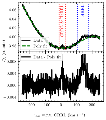
Figure 2: Example of the baseline removal process for the GBT observations. Upper panel: Raw data (in black) and the polynomial (green dashed line) used to remove the shape of the bandpass from the data. In this example a polynomial of order five was used. The red and blue dotted lines show the ranges where we expect the RRLs. These ranges are not considered while fitting the polynomial. Bottom panel: Data after subtraction of the polynomial used to capture the bandpass shape. The velocity axis is referenced with respect to the rest frequency of the corresponding CRRL. This data is part of project AGBT12A_484.

The data was exported to SDfits format from the NRAO archive. The observations were calibrated to a temperature scale using the hot load on the GBT and its temperature, as listed in the SDfits header. To remove the continuum and any large-scale ripples in the spectra we fitted a polynomial to line-free channels. For $97.5\%$ of the spectra an order five polynomial was used, for $2\%$ an order nine polynomial, and for the remaining an order $11$ polynomial. If a polynomial with an order greater than $11$ was required, the data was flagged as bad and not used. Line-free channels are defined as those that have velocities less than $-5$ km s^-1 and greater than $180$ km s^-1, and those between $25$ km s^-1 and $100$ km s^-1, where the velocities quoted are with respect to the rest frequency of the corresponding CRRL. An example of the polynomial fitting is shown in Figure 2. In this example a polynomial of order five was used to remove the continuum and the large-scale ripples. In some cases the spectral window was flagged and marked as bad because of strong RFI. The remaining spectra that showed no obvious artifacts were then stacked to improve the signal-to-noise ratio.

In the pointing observations present in the archive, we found no corresponding observations of a reference region. For this reason we did not try to estimate the continuum temperature of the source from these observations.

2.2 LOFAR observations

We observed Orion A with the Low Frequency Array (LOFAR, van Haarlem et al. 2013) during two separate projects, two years apart. The observations were carried out on February $2$, $2014,$ and October $27$, $2016$. Both observations used the high band antennas (HBA) in their low frequency range ($110$–$190$ MHz). The number of Dutch stations available was $34$ for both observations.

Complex gain solutions were derived on 3C147 and then transferred to the target field, following a first generation calibration scheme (e.g., Noordam & Smirnov 2010). We adopted the Scaife & Heald (2012) flux scale. The calibrated visibilities were then imaged and cleaned. During the inversion a Briggs weighting was used, with a robust parameter of $0$ (Briggs 1995). The cubes have a synthesized beam of $3\aas@@fstack{\prime}65\times 2\arcmin$ at a position angle of $166\degr$. Given the shortest baseline present in the visibilities, $130$ m, the LOFAR observations are sensitive to emission on angular scales smaller than $53\arcmin$.

From the cubes we extracted a spectrum from a $9\arcmin\times 9\arcmin$ region centered on M42. For the $2014$ observations, $20$ spectral windows were stacked resulting in a spectrum with a spectral resolution of $7$ km s^-1. This resulted in a detection of the C$351\alpha$ line in absorption with a signal-to-noise ratio of $4.5$. For the $2016$ observations, $22$ spectral windows were stacked. In general, the data quality for the $2016$ observations was worse than in the $2014$ observations by a factor $2\mbox{--}4$. In the $2016$ observations we found an absorption feature with a signal-to-noise ratio of $2.5$. A comparison of the observed line profile for both observations is presented in Figure 3. The line properties are consistent between the two observations. Based on this, we are confident that the detected absorption feature, which we associate with the C$351\alpha$ line, is of astronomical origin.

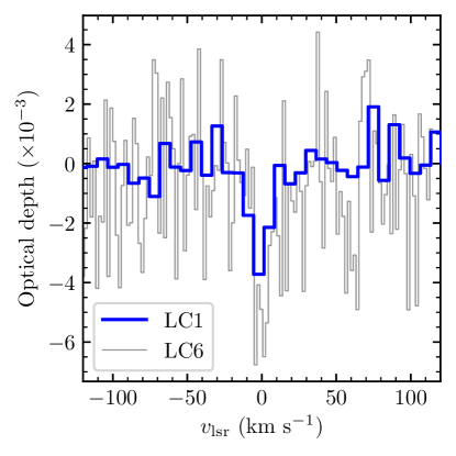
Figure 3: LOFAR spectra of C$351\alpha$ observed on two different nights. The blue steps show the spectra obtained from observations performed during February $2014$ and the gray steps for observations taken during October $2016$. The $2014$ detection, with a signal-to-noise ratio of $4.5$, is confirmed by the $2016$ observations (with a signal-to-noise ratio of $2.5$). The spectra are the spatial average over a $9\arcmin\times 9\arcmin$ box centered on M42.

2.3 Literature data

We also use observations of CRRLs and other tracers of the ISM from the literature. The CRRL observations include the C$65\alpha$ map of a $5\arcmin\times 5\arcmin$ region close to M42 at a spatial resolution of $40\arcsec$, the intensity of the C$91\alpha$ line towards a region to the north of Orion-KL (Wyrowski et al. 1997), and observations of the C$30\alpha$ line using the Atacama Large Millimeter Array (ALMA) total power array plus ALMA compact array (ACA) at a spatial resolution of $28\arcsec$ (Bally et al. 2017). Throughout this work we compare the CRRL observations with the $158$ $\mu$m-[CII] line cube observed with the Stratospheric Observatory for Infrared Astronomy (SOFIA Young et al. 2012) upGREAT receiver (Heyminck et al. 2012; Risacher et al. 2016). This cube has a spatial resolution of $18\arcsec$ and a velocity resolution of $0.2$ km s^-1, and covers a region of roughly $1\degr\times 1\degr$. The observations and reduction used to produce the $158$ $\mu$m-[CII] line cube are described in detail in Pabst et al. (2019). Additionally, we compare the CRRL cubes with observations of ¹²CO$(2\mbox{--}1)$ and ¹³CO$(2\mbox{--}1)$ (Berné et al. 2014), and with the dust properties as derived from Herschel and Planck observations (Lombardi et al. 2014).

3 Results

In this section we start by describing the RRL spectra towards M42, focusing on the CRRLs. Then we present the maps of CRRL emission that we used to study the spatial distribution of the lines and for comparison with other tracers of the ISM, particularly the $158$ $\mu$m-[CII] line.

3.1 RRLs from M42

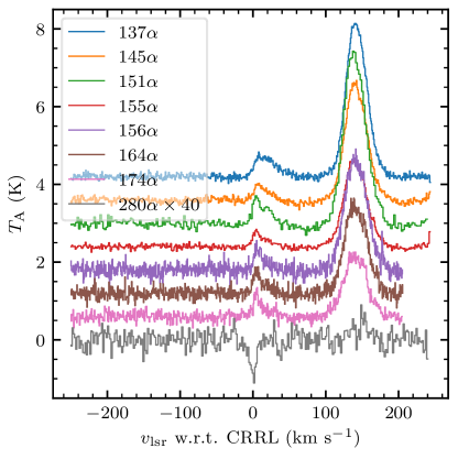
Figure 4: Hydrogen, helium, and carbon radio recombination lines observed with the GBT for $\alpha$ lines (the change in principal quantum number is $\Delta n=1$) with principal quantum numbers $137$, $145$, $151$, $155$, $156$, $164$, $174$, and $280$. The velocity is given with respect to the CRRL. To reference the velocity with respect to helium or hydrogen, $27.4$ km s^-1 or $149.4$ km s^-1, respectively, is subtracted. The spectra are offset by a constant $0.7$ K, and the $280\alpha$ spectrum is scaled by a factor of $40$. This data is part of project AGBT02A_028. Since all the observations are obtained using the same telescope, their spatial resolution ranges from $4\aas@@fstack{\prime}4$ to $36\arcmin$.

Some of the RRL stacks obtained from the pointed observations towards M42 are presented in Figure 4. In these stacks the strongest features are hydrogen RRLs (HRRLs), followed by a blend of CRRLs and helium RRLs (HeRRLs). The velocity difference between HeRRLs and CRRLs is $27.4$ km s^-1, and between HRRLs and CRRLs is $149.4$ km s^-1. HRRLs and HeRRLs trace the ionized gas in the HII region, for which the line FWHM due to Doppler broadening is $\approx 20$ km s^-1. In M42 the ionized gas is blueshifted with respect to the bulk of the molecular and neutral gas (e.g., Zuckerman 1973; Balick et al. 1974a, b). This brings the HeRRL and CRRL closer, resulting in the observed blending. Fortuitously, we can use the fact that the HeRRLs are broader to distinguish them from the CRRLs.

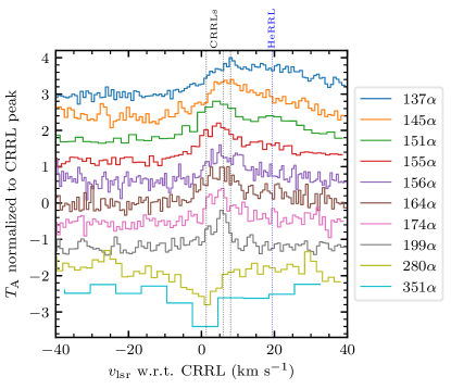
Figure 5: Zoom-in of RRL spectra towards M42 around the carbon feature. The RRLs correspond to $\alpha$ lines with principal quantum numbers $137$, $145$, $155$, $156$, $164$, $174$, $199$, $280$, and $351$. CRRLs with $n\leq 199$ appear in emission, while those with $n\geq 280$ appear in absorption. The velocity is given with respect to the CRRL and the intensity axis is normalized to the peak of the CRRL. To reference the velocity with respect to helium, $27.4$ km s^-1 was subtracted. The spectra are offset by a constant $0.6$ and are normalized using the peak of the brightest CRRL in each spectra. The dotted lines indicate the position of the CRRLs at $\approx 1.3$ km s^-1, $\approx 6$ km s^-1, and $\approx 8$ km s^-1 (black) and the HeRRL (blue). The C$351\alpha$ spectrum is the spatial average over a circle $36\arcmin$ in diameter centered on M42.

Before focusing on the CRRLs we use the strength of the HRRLs to estimate the accuracy of the temperature scale: HRRLs of similar principal quantum number have similar properties. Then we can quantify the accuracy of the temperature scale by comparing the temperature of H$n\alpha$ lines of similar principal quantum number. The peak temperatures of the HRRLs presented in Figure 4 show variations of up to $25\%$ between adjacent stacks (see Table 4). For example, the peak temperature of the H$155\alpha$ line should be almost the same as that of the H$156\alpha$ line, but they differ by $22\%$. Based on this we conclude that the calibration using the noise diode has an accuracy of about $25\%$.

As pointed out above, the CRRLs can be identified as a narrow feature on top of the broader HeRRLs in Figure 4. A zoom-in of the CRRLs is presented in Figure 5. One of the most notable features in the spectra of Figure 5 is the transition of the lines from emission to absorption between the C$199\alpha$ and C$280\alpha$ lines. Towards M42, this is the first time that CRRLs have been observed in absorption.

In terms of the velocity structure of the CRRLs, we can identify at least two velocity components in emission at $6$ and $8$ km s^-1. The $\approx 8$ km s^-1 velocity component can be observed in the C$137\alpha$ RRL, while the $\approx 6$ km s^-1 velocity component can be observed in the CRRLs with $n=145\mbox{--}199$. Gas with a velocity of $\approx 8$ km s^-1 is associated with the background molecular cloud, while gas with lower velocities is associated with foreground gas (e.g., Dupree 1974; Ahmad 1976; Boughton 1978). In the case of this line of sight the foreground gas corresponds to the Veil, which is less dense ($n_{\mathrm{H}}\sim 10^{3}$ cm^-3 Abel et al. 2016) and irradiated by a weaker radiation field (e.g., Abel et al. 2016) than the PDR that forms between the HII region and Orion A ($n_{\mathrm{H}}\sim 10^{5}$ cm^-3; e.g., Natta et al. 1994).

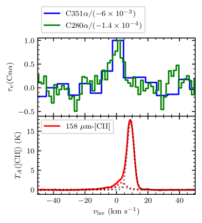
Figure 6: Comparison between the CRRLs observed in absorption and the $158$ $\mu$m-[CII] line. The blue steps show the C$351\alpha$ line profile inverted (from the LOFAR observations in $2014$), the green steps the C$280\alpha$ line inverted (from the GBT observations AGBT02A_028), and the red steps show the $158$ $\mu$m-[CII] line (from the SOFIA observations of Pabst et al. 2019). The CRRLs trace a fainter velocity component in the $158$ $\mu$m-[CII] line due to the effect of stimulated emission. The dotted lines in the lower panel show the best fit Gaussian line profiles used to decompose the $158$ $\mu$m-[CII] line (the properties of these components are given in Table 6). The spectra are the spatial average over a circle $36\arcmin$ in diameter centered on M42.

For the C$174\alpha$ and C$199\alpha$ lines there are hints of emission at $\approx 2$ km s^-1. CRRL emission at this velocity has not been reported previously, though some authors reported the detection of unidentified RRLs at velocities of $\approx-3$ km s^-1 (Chaisson & Lada 1974) and $\approx-0.6$ (Pedlar & Hart 1974). Given that the $\approx 2$ km s^-1 velocity component is detected in two independent observations (the C$174\alpha$ stack is part of project AGBT02A_028, while the C$199\alpha$ stack is part of AGBT12A_484), we consider the features to be CRRLs. The C$174\alpha$ and C$199\alpha$ lines at $\approx 2$ km s^-1 trace gas in component B of the Veil.

To compare the lines in absorption we use an aperture of $36\arcmin$, similar to the resolution of the observations used to produce the C$280\alpha$ detection ($40\arcmin$, Table 5). The inverted spectra are presented in Figure 6. The C$280\alpha$ line has a velocity centroid of $0.7\pm 1.0$ km s^-1 (Table 4), while the C$351\alpha$ line has a velocity centroid of $2.3\pm 0.8$ km s^-1. These lines trace the expanding Veil.

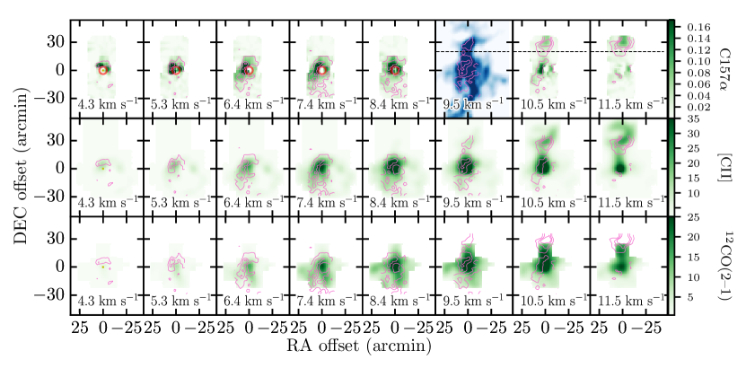
Figure 7: Channel maps of C$157\alpha$ (top row), $158$ $\mu$m-[CII] (middle row), and ¹²CO$(2\mbox{--}1)$ (bottom row) line emission. The pink contours show C$157\alpha$ emission above $3\sigma$ in steps of $3\sigma$, with $\sigma$ being the standard deviation of the spectra ($\sigma\approx 10$ mK). The velocity is indicated at the bottom of each panel. All cubes have been convolved to a spatial resolution of $8\aas@@fstack{\prime}1$. The velocity axes were averaged to match the velocity resolution of the C$157\alpha$ cube. The spatial axes are given in offset with respect to M42. The red circle shows the extent of M42 in the $21$ cm continuum map of van der Werf et al. (2013). In the top panel with a velocity of $9.5$ km s^-1 the background image in blue is the $857$ GHz emission as observed with Planck at $4\aas@@fstack{\prime}6$ resolution (Planck Collaboration et al. 2016). In the top row panels with a velocity $\geq 9.5$ km s^-1, the dashed line shows a Declination of $-5.0583\degr$ (J2000), used to separate S279 from Orion A. The color scales at the right are in units of K.

The $158$ $\mu$m-[CII] line spectrum extracted from the $36\arcmin$ aperture used to study the C$280\alpha$ and C$351\alpha$ lines is also shown in Figure 6. There we see that the Veil ($v\approx 3$ km s^-1) has a peak antenna temperature of $\approx 1.8$ K, while that from the background PDR ($v\approx 9$ km s^-1) is a factor of ten stronger. The Veil is weaker in the $158$ $\mu$m-[CII] line because it is farther from the Trapezium ($\approx 2$ pc; Abel et al. 2016) and hence colder.

3.2 Spatial distribution of CRRLs

3.2.1 $\mathrm{C}157\alpha$

The spatial distribution of a stack of CRRLs with $n=156\mbox{--}158$ (with an effective $n=157$) is presented in Figure 7 in the form of channel maps. In Figure 7 we also include channel maps of $158$ $\mu$m-[CII] and ¹²CO$(2\mbox{--}1)$ at the same resolution. The channel maps show that the C$157\alpha$ emission avoids the regions where the $18$ cm continuum is brightest. At the frequency of the C$157\alpha$ line ($\approx 1.6$ GHz) the brightest portions of the HII region are optically thick (e.g., Wilson et al. 2015). This means that radiation coming from the interface between the background cloud and the HII region is heavily attenuated at these frequencies. Moreover, the noise is greater towards the HII region due to its contribution to the antenna temperature.

At velocities of less than $6$ km s^-1 the C$157\alpha$ emission comes from regions close to the Northern Dark Lane and the Dark Bay. The Northern Dark Lane is a dark structure that separates M42 from M43 in optical images (see Figure 12 in O’Dell & Harris 2010). The Dark Bay is a region of high optical extinction which seems to start in the Northern Dark Lane and extends to the southwest in the direction of the Trapezium stars. These structures are also seen in the lines of $158$ $\mu$m-[CII] and ¹²CO$(2\mbox{--}1)$. At velocities in the range $6$ km s^-1 to $7.4$ km s^-1 the C$157\alpha$ emission extends to the south of M42, following the limb brightened edge of the Veil (Pabst et al. 2019). Then at $8.4$ km s^-1 the C$157\alpha$ emission seems to trace the Orion molecular cloud 4 (OMC4, e.g., Berné et al. 2014). At velocities higher than $9$ km s^-1 we see C$157\alpha$ emission extending to the north of M42. At $10$ km s^-1 we see part of the HII region S279 in the northernmost portion of the map (at an offset of $30\arcmin$ to the north), containing the reflection nebulae NGC 1973, 1975, and 1977. In general, the spatial distribution of the C$157\alpha$ emission follows that of $158$ $\mu$m-[CII] and to a lesser extent that of ¹²CO$(2\mbox{--}1)$. Then C$157\alpha$ emission predominantly traces the northern part of the ISF (see the top panel in Figure 7 for $v_{\mathrm{lsr}}=9.8$ km s^-1).

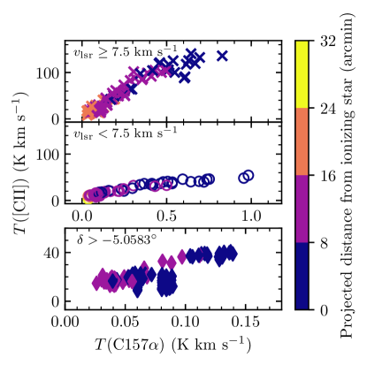
Figure 8: $158$ $\mu$m-[CII] line intensity as a function of the C$157\alpha$ line intensity. The line emission is separated into different groups based on known features in the maps. The top panel shows line emission with velocity in the range $[4,7.5)$ km s^-1 and declination below $-5.0583\degr$, associated with the Veil; the middle panel shows line emission with velocity in the range $[7.5,12)$ km s^-1 and declination below $-5.0583\degr$, associated with the ISF; and the bottom panel shows line emission at declination above $-5.0583\degr$, associated with S279.

To further explore the relation between the FIR [CII] line and the C$157\alpha$ line we compare their intensities at each position in the map. We select pixels that show C$157\alpha$ emission with a signal-to-noise ratio $\geq 5$ in the velocity range $4\mbox{--}12$ km s^-1. We split the selected pixels into three groups that separate different components in Orion A. The first group aims to trace gas along the ISF. For this group we select pixels with line emission in the velocity range $7.5\leq v_{\mathrm{lsr}}<12$ km s^-1 and with a declination below $-5.0583\degr$ (J2000). The second group targets gas that is associated with the Veil. Pixels with line emission in the velocity range $4\leq v_{\mathrm{lsr}}<7.5$ km s^-1 and a declination below $-5.0583\degr$ (J2000) are selected in this group. The third group targets gas associated with S279. In this group, pixels with a declination above $-5.0583\degr$ (J2000) are selected.

The $158$ $\mu$m-[CII] and C$157\alpha$ line intensities for the different groups are presented in Figure 8. Here we can see that there is a relation between the intensities of both lines, and that the shape of their relation depends on which velocity structure is selected. Gas associated with the ISF reaches a higher $158$ $\mu$m-[CII] line brightness than that in the other groups (the Veil or S279). The shape of the relation for the gas associated with S279 looks like a scaled-down version of that in the ISF. For the gas in the Veil, the C$157\alpha$ line is brighter than in the ISF or S279 at similar $158$ $\mu$m-[CII] brightness temperature, because the Veil is in front of the continuum source.

In Figure 8 we have also color-coded the data as a function of their projected distance from the ionizing star. For the gas in the ISF and the Veil, $\Theta^{1}$ Ori C (HD 37022) is the ionizing star, while for gas in S279 it is $42$ Ori (HD 37018, c Ori); $\Theta^{1}$ Ori C is a O7 star, while $42$ Ori is a B1 star (Hoffleit & Warren 1995). There is a trend in the line brightness as a function of distance from the ionizing star; closer to the ionizing source the lines are brighter.

In the CRRL spectra of Figure 5 we can see that as the frequency decreases (increasing $n$), the velocity centroid of the emission lines shifts from $\approx 9$ km s^-1 to $\approx 6$ km s^-1 and additional velocity components are more easily observed at lower frequencies (e.g., at $2$ km s^-1). This is due to a combination of effects. First, the dominant emission mechanism changes as a function of frequency. At higher frequencies spontaneous emission dominates, while at lower frequencies stimulated transitions become dominant (Sect. 4.1.4). Spontaneous emission lines are brighter from denser regions (i.e., the background PDR), while to get stimulated transitions a bright background continuum is required. Second, all the observations were obtained using the same telescope, hence the observing beam becomes larger with decreasing frequency, and therefore different gas structures are included in the beam. As Figure 7 shows, the velocity distribution of the gas is such that gas with lower velocities has a higher emission measure around M42 than towards M42 itself. This implies that at higher frequencies we mainly see CRRLs from the background PDR since this is the densest component along the line of sight, while at lower frequencies we observe the gas around and in front of M42.

3.2.2 $\mathrm{C}30\alpha$

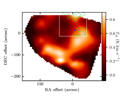
Figure 9: Moment $0$ maps of C$30\alpha$ emission and C$65\alpha$ emission. The green contours show the C$30\alpha$ emission at values of $40$, $60,$ and $80$ mK km s^-1. The color map shows the C$65\alpha$ emission (Wyrowski et al. 1997). The spatial resolution of the C$30\alpha$ map is $28\arcsec$, while that of the C$65\alpha$ map is $40\arcsec$. A white box shows the extent of the region mapped by ALMA where C$30\alpha$ is detected (southeast map in Bally et al. 2017). The spatial axes are given in offset with respect to M42, and a blue star indicates the position of $\Theta^{1}$ Ori C.

We searched for CRRLs in the ALMA cubes presented by Bally et al. (2017). These cubes contain $\alpha$ RRLs with $n=30$ within the observed frequency range. The H$30\alpha$, He$30\alpha$, and C$30\alpha$ lines are detected in the cube that covers the southeast region of the Orion Molecular Core 1. We confirm that the observed line is C$30\alpha$ by comparing its velocity integrated intensity (moment $0$) with that of the C$65\alpha$ line at a similar angular resolution ($40\arcsec$, Wyrowski et al. 1997). The comparison is presented in Figure 9, where we can see the C$30\alpha$ emission overlapping with the C$65\alpha$ emission over the region mapped. This confirms that the emission corresponds to C$30\alpha$ and not to a molecular line at a similar velocity.

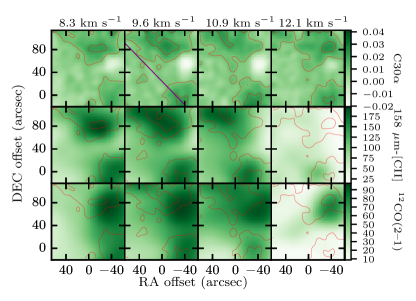
Figure 10: Channel maps of C$30\alpha$ (top row), $158$ $\mu$m-[CII] (middle row), and ¹²CO$(2\mbox{--}1)$ (bottom row) line emission. The red contours show C$30\alpha$ emission above $10$ mK, in steps of $10$ mK. The velocity with respect to the local standard of rest is indicated at the top of each row. All cubes have been convolved to a spatial resolution of $28\arcsec$. The velocity axes were averaged and then linearly interpolated to match the velocity axis of the C$30\alpha$ cube. The spatial axes are given in offset with respect to M42. In the C$30\alpha$ panel with a velocity of $9.6$ km s^-1 a solid purple line shows the slice used to extract the brightness profile presented in Figure 11.

Next we examine how the C$30\alpha$ emission is distributed with respect to the $158$ $\mu$m-[CII] and ¹²CO$(2\mbox{--}1)$ lines. This comparison is presented in Figure 10. The distribution of C$30\alpha$ resembles that of the other two lines, but there are differences between them.

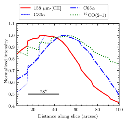
Figure 11: Comparison of the intensities of the C$30\alpha$, $158$ $\mu$m-[CII] (Pabst et al. 2019), and ¹²CO$(2\mbox{--}1)$ (Berné et al. 2014) lines. The thin dashed blue line shows the C$30\alpha$ line profile, the blue dash-dotted line for the C$65\alpha$ line, the red solid line for the $158$ $\mu$m-[CII] line, and the green dotted line for the ¹²CO$(2\mbox{--}1)$ line. The slice from where the velocity integrated brightness profiles was extracted is shown in Figure 10. The position of $\Theta^{1}$ Ori C marks the origin of the distance scale.

To illustrate the above point we extract the line intensity from a slice that joins $\Theta^{1}$ Ori C with the peak of C$30\alpha$ emission in the south of the map (purple line in Figure 10). To produce the intensity profiles the cubes are integrated over the velocity range $8$ km s^-1 to $12$ km s^-1, and the result is presented in Figure 11. There we can see that the $158$ $\mu$m-[CII] line peaks closer to $\Theta^{1}$ Ori C than the ¹²CO$(2\mbox{--}1)$ line and the CRRLs. This arrangement is similar to the layered structure found in a PDR (e.g., Wyrowski et al. 2000).

3.3 PDR models

To understand the relation between the gas traced by the $158$ $\mu$m-[CII] line and that traced by the CRRLs we use a PDR model. In this case we use the Meudon PDR code (Le Petit et al. 2006) to generate temperature and density profiles. To model the PDR we adopt a total extinction of $A_{V}=20$ along the line of sight and a constant thermal pressure throughout the gas slab. How far the UV radiation penetrates into the PDR is largely determined by the extinction curve, which towards $\Theta^{1}$ C Ori is almost flat with an extinction-to-color index $R_{V}=5.5$ (Fitzpatrick & Massa 1988; Cardelli et al. 1989). The extinction-to-column density ratio ($A_{V}/N_{\mathrm{H}}$) is determined from the extinction observed towards the Trapezium stars, $A_{V}=2.13\pm 0.52$ (Ducati et al. 2003), and the hydrogen column density towards $\Theta^{1}$ Ori C and B of $N_{\mathrm{H}}=4.4\times 10^{21}$ cm^-2 (Shuping & Snow 1997; Cartledge et al. 2001). We adopt a carbon abundance of [C/H]$=1.4\times 10^{-4}$, measured against $\Theta^{1}$ Ori B (Sofia et al. 2004). The models are illuminated by the ISRF on the far side ($A_{V}=20$) scaled to $G_{0}=1$ using the parametrization of Mathis et al. (1983). On the observer side ($A_{V}=0$) we vary the strength of the ISRF to explore its effect on the gas properties.

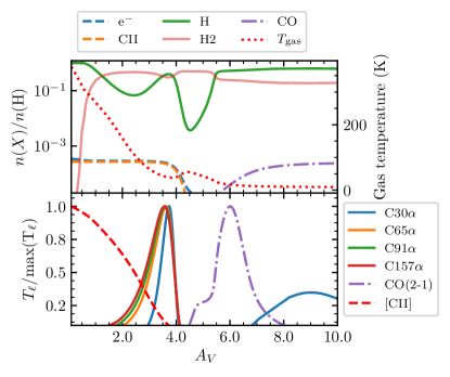
Figure 12: Example of temperature and abundance profiles obtained with the Meudon PDR code. The top panel shows the gas temperature and abundances, while the bottom panel shows the line brightness temperature of C$n\alpha$ lines with principal quantum numbers $n=30,\,65,\,91\,\mbox{and}\,157$, and of the $158$ $\mu$m-[CII] line. The input conditions for the model are a radiation field of $G_{0}=1\times 10^{4}$, in Mathis units, and a total gas density of $n_{\mathrm{H}}=1\times 10^{4}$ cm^-3. The difference between the abundance of free electrons and the abundance of ionized carbon is produced by the ionization of species such as sulfur or hydrogen.

Once we have computed the temperature and density in the PDR, we process the output to determine how much of the $158$ $\mu$m-[CII] and CRRL brightness comes from different layers in the PDR. The different layers represent different depths into the molecular cloud and are expressed in terms of the visual extinction $A_{V}$. Examples of the temperature and density profiles, and of the line brightness contributed from each layer in the PDR, are presented in Figure 12. For this model we used an incident radiation field of $G_{0}=1\times 10^{4}$, in Mathis units, and a total gas density of $n_{\mathrm{H}}=1\times 10^{4}$ cm^-3. The layered structure in the models is in good agreement with observations of CRRLs and the $158$ $\mu$m-[CII] line for the PDRs associated with the Orion Bar and NGC 2023 (Wyrowski et al. 1997, 2000; Bernard-Salas et al. 2012; Sandell et al. 2015).

We use the models of Salgado et al. (2017a) to compute the properties of the CRRLs. These models solve the level population equations taking into account deviations from local thermodynamical equilibrium (LTE). The deviation from LTE in the population of carbon atoms is characterized by the factor $b_{n}$ and the effect of stimulated emission by the factor $\beta_{nn^{\prime}}$ (e.g., Shaver 1975; Salgado et al. 2017a). These are known as departure coefficients. The models of Salgado et al. (2017a) include the effect of dielectronic capture (Watson et al. 1980; Walmsley & Watson 1982). This effect will produce an overpopulation at $n$ levels in the range $30$–$500$ with respect to a system that does not undergo dielectronic capture. For conditions like those found towards Orion A ($n_{\mathrm{H}}\sim 10^{5}$ and $T\sim 100$ K, e.g., Natta et al. 1994), dielectronic capture will produce twice as many atoms with an electron at $n=91$ than if we ignore its effect. The effect of dielectronic capture has not been considered explicitly before when studying the Orion A region, but it has been suggested that it could help explain the observed line ratios (Wyrowski et al. 1997). We note that when solving the level population problem we do not include the presence of a free-free radiation field. For hydrogen atoms, the departure coefficients will change by less than $12\%$ for $n$ between $10$ and $60$ (e.g., Prozesky & Smits 2018). The effect is smaller for $n>60$.

For a homogeneous slab of gas in front of a continuum source, the intensity of a CRRL, $T_{\ell}\Delta\nu$, is given by (e.g., Dupree 1974)

$$T_{\ell}\Delta\nu=\tau^{*}_{\ell}\Delta\nu(b_{n^{\prime}}T_{\mathrm{e}}-b_{n}\beta_{nn^{\prime}}T_{\mathrm{cont}}),$$ (1)

where $\tau^{*}_{\ell}$ is the line optical depth in LTE, $T_{\mathrm{e}}$ the electron temperature of the gas, and $T_{\mathrm{cont}}$ the temperature of the background continuum. In this equation, the first term in parentheses corresponds to the contribution to the line brightness temperature from spontaneous emission, while the second term represents the contribution from stimulated emission. The line optical depth in LTE is given by (e.g., Salgado et al. 2017b)

$$\tau^{*}_{\ell}\Delta\nu=1.069\times 10^{7}\Delta nMT_{\mathrm{e}}^{-2.5}e^{\chi_{n}}EM_{\mathrm{C}^{+}}\,\mbox{Hz},$$ (2)

where $\Delta n=n^{\prime}-n$, $M$ is the oscillator strength of the transition (Menzel 1968), $\chi_{n}=157800n^{-2}T^{-1}_{\mathrm{e}}$, and $EM_{\mathrm{C}^{+}}=n_{\mathrm{e}}n_{\mathrm{C}^{+}}L$ is the ionized carbon emission measure in pc cm^-6 with $L$ the thickness of the slab.

To compute the CRRL brightness temperature from the PDR we assume that the emission is due to spontaneous emission with no background continuum (Natta et al. 1994). In each layer the temperature and electron density determine the value of $b_{n}$. For the CRRLs the $b_{n}$ values are $<1$ over the range of physical properties explored here. The line brightness in the LTE case is, on average, $50\%$ larger than in the non-LTE case. The difference between the LTE and non-LTE cases is larger for lower pressures and higher radiation fields. In an extreme case the LTE value is $70\%$ higher than the non-LTE value.

To compute the $158$ $\mu$m-[CII] line brightness temperature we use the equations provided in Appendix B of Tielens & Hollenbach (1985) and the collisional excitation rates provided in Goldsmith et al. (2012). The equations in Tielens & Hollenbach (1985) provide the line intensity with a correction for the finite optical depth of the line.

In Figure 12 we can see that most of the $158$ $\mu$m-[CII] line comes from the surface layers of the PDR ($A_{V}<3.5$), while the CRRL emission comes from a deeper layer ($A_{V}=3.5$). The gas temperature can be a factor of $10$ lower at $A_{V}=3.5$ with respect to $A_{V}<3.5$. This shows that the CRRL optical depth has a stronger dependence on the temperature ($\propto T^{-5/2}$) than that of the $158$ $\mu$m-[CII] line. Therefore, when we constrain the gas physical properties using CRRLs and the $158$ $\mu$m-[CII] line using a uniform gas slab model, the temperature and density will be an average between the properties of the layers traced by the two lines. We also note that the studied CRRLs trace an almost identical layer in the PDR, which justifies using their line ratios regardless of geometry. The situation is similar for PDRs with $10^{2}<G_{0}\leq 10^{5}$ and $10^{2}$ cm${}^{-3}<n_{\mathrm{H}}\leq 10^{6}$ cm^-3.

The structure observed in Figure 12 is similar to that found in Figure 11. There, we observe that the separation between the peak of the $158$ $\mu$m-[CII] line is offset by $\approx 10\arcsec$ with respect to the peak of ¹²CO$(2\mbox{--}1)$. For a distance of $417$ pc, this translates to a projected separation of $0.02$ pc. Using the result of Figure 12, we have that the separation between these tracers corresponds to roughly $A_{\mathrm{V}}=6$ or $N_{\mathrm{H}}=1.2\times 10^{22}$ cm^-2. This corresponds to a hydrogen density of $2\times 10^{5}$ cm^-3, similar to that found in the interclump medium in the Orion Bar ($5\times 10^{4}$ cm^-3 Young Owl et al. 2000 or $2\times 10^{5}$ cm^-3 Simon et al. 1997). This hydrogen density is also consistent with the value found towards a nearby region using CRRL and [CII] ratios (Sect. 4.2.3).

4 Physical conditions

In this section we use CRRLs and the $158$ $\mu$m-[CII] line to determine the physical conditions of the gas, for example its temperature and density. We do this by modeling the change in the properties of the CRRLs as a function of principal quantum number (e.g., Ahmad 1976; Boughton 1978; Jaffe & Pankonin 1978; Payne et al. 1994; Oonk et al. 2017; Salas et al. 2018), and by comparing the CRRLs with different principal quantum numbers to the $158$ $\mu$m-[CII] line.

4.1 The Veil towards M42

To study the Veil of Orion we focus on the information provided by the CRRLs observed in absorption and the C$157\alpha$ emission at velocities $\lesssim 7$ km s^-1.

4.1.1 Transition from emission to absorption

For the CRRLs associated with the Veil the largest principal quantum number for which the line is observed in emission is $n=199$ (Figure 5). Then at $n=280$ the line is observed in absorption. This sets a lower limit to the electron density of the gas of $n_{\mathrm{e}}\geq 0.03$ cm^-3, and for the electron temperature $35\leavevmode\nobreak\ \mbox{K}\leq T_{\mathrm{e}}\leq 130$ K. The constraint on the gas properties set by the transition from emission to absorption is shown in Figure 13 as a purple dashed line.

4.1.2 CRRL ratio

The ratio of two CRRLs in absorption provides an additional constraint to determine the gas properties (e.g., Salgado et al. 2017b; Salas et al. 2017, 2018). Here we use the ratio of the integrated optical depths of the C$280\alpha$ and C$351\alpha$ lines to constrain the gas temperature and electron density.

In order to convert the observed C$280\alpha$ line temperature to optical depth, we need to estimate the continuum adjacent to the line. As mentioned in Section 2.1.2, we chose not to directly estimate the continuum from the observations used to produce the C$280\alpha$ spectrum as we do not have a reference position to use to estimate the contribution from non-astronomical sources to the antenna temperature. Instead, we use the low frequency spectrum of M42 to estimate the contribution to the continuum in the C$280\alpha$ spectrum. Using the Very Large Array (VLA, Napier et al. 1983) in its D configuration (minimum baseline $35$ m), Subrahmanyan et al. (2001) observed M42 at $330$ MHz. They measured a total combined flux for M42 and M43 (which is only $\sim 5\arcmin$ away from M42) of $167\pm 5$ Jy, consistent with single dish measurements (e.g., Lockman & Brown 1975). We assumed that the combined flux density from M42 and M43 scales as $S_{\nu}\propto\nu^{0.92\pm 0.08}$ between $240$ and $400$ MHz (based on the continuum measurements presented in Lockman & Brown 1975). We estimated the effect of beam dilution on the measured antenna temperature for the continuum using the $330$ MHz continuum maps (Subrahmanyan et al. 2001). In these maps, M42 and M43 cover a circular area with a radius of $18\arcmin$ centered at $(\alpha,\delta)_{\mathrm{J2000}}=(5^{\mathrm{h}}35^{\mathrm{m}}00^{\mathrm{s}},-5\degr 25^{\mathrm{m}}22^{\mathrm{s}})$. The $330$ MHz continuum shows a structure similar to that of the LOFAR $149$ MHz continuum map. The beam of the C$280\alpha$ observations covers most of this region, and leaves out less than $0.4\%$ of the continuum flux. Therefore, we estimated that at $298$ MHz the continuum temperature of the C$280\alpha$ spectra will be $195\pm 6$ K. Ultimately, we find the integrated optical depth of the C$280\alpha$ line is $1.4\pm 0.2$ Hz.

Table 3: Veil line properties

Line	$v_{\mathrm{lsr}}$	$T_{\mathrm{line}}$	$\Delta v$(FWHM)
	(km s-1)	(K)	(km s-1)
[CII]	$8.98\pm 0.01$	$17.58\pm 0.07$	$5.02\pm 0.01$
	$3.2\pm 0.1$	$1.82\pm 0.05$	$6.6\pm 0.2$
	$-0.1\pm 0.4$	$0.70\pm 0.04$	$17.9\pm 0.5$
C$280\alpha$	$0.7\pm 1.0$	$-0.023\pm 0.003$	$11\pm 1$
C$351\alpha$	$2.3\pm 0.8$	$-0.0061\pm 0.0008$	$10\pm 1$

The ratio of the integrated optical depths of the C$280\alpha$ and C$351\alpha$ lines is $(4\pm 1)\times 10^{-2}$. The constraint on the gas temperature and electron density set by this ratio is shown in Figure 13 with blue dashed lines. A higher ratio implies a higher temperature. In this case, the integrated optical depth ratio poses a more stringent constraint on the gas properties than the point at which the lines transition from emission to absorption.

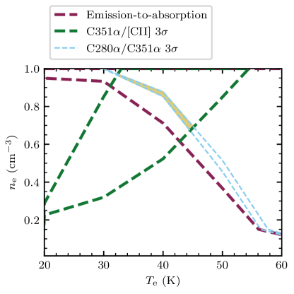
Figure 13: Constraints on the temperature and electron density for gas associated with Orion’s Veil. The dashed lines show the constraints on the gas properties derived from different observables: the transition of the CRRLs from emission to absorption between $n=200$ and $279$ (purple); the ratio of the integrated optical depths of the C$280\alpha$ and C$351\alpha$ lines (light blue); the ratio of the C$351\alpha$ velocity integrated optical depth to the $158$ $\mu$m-[CII] line intensity (green). All the constraints shown are $3\sigma$ ranges. The region where the constraints overlap is shown as a yellow shaded region, close to $0.9$ cm^-3 and $40$ K.

4.1.3 CRRLs and FIR [CII] line

Here we compare the latest $158$ $\mu$m-[CII] line maps of Pabst et al. (2019) with the CRRLs observed in absorption. The cube of Pabst et al. (2019) presents the $158$ $\mu$m-[CII] line resolved in velocity and samples a region larger than that studied in CRRLs. With this we were able to perform a direct comparison between the lines over the same regions without making assumptions about their velocity structure. Previous comparisons between CRRLs and the $158$ $\mu$m-[CII] line were performed using observations that did not resolve the velocity structure and/or did not sample the same spatial regions (e.g., Natta et al. 1994; Smirnov et al. 1995; Salas et al. 2017).

Here, we compare the C$351\alpha$ line with the $158$ $\mu$m-[CII] line over the same spatial regions. Since the C$351\alpha$ line is observed in absorption, it will only trace gas that is in front of the continuum source. Then the $158$ $\mu$m-[CII] line spectrum used to make a comparison with the C$351\alpha$ line should be extracted from a region that encompasses the continuum source. This corresponds to a circular region with a radius of $18\arcmin$ centered at $(\alpha,\delta)_{\mathrm{J2000}}=(5^{\mathrm{h}}35^{\mathrm{m}}00^{\mathrm{s}},-5\degr 25^{\mathrm{m}}22^{\mathrm{s}})$. The absorption spectra will be weighted by the underlying continuum, whereas the $158$ $\mu$m-[CII] line will not be. Hence, even if we use an aperture that covers most of the continuum emission, the lines could trace different portions of the Veil.

The resulting $158$ $\mu$m-[CII] line spectrum (Figure 6) shows the presence of at least three velocity components. We fitted three Gaussian components corresponding to the Veil, the dense PDR, and the HII region. The best fit parameters of the Gaussian profiles are presented in Table 6. Using the values for the component associated with the Veil, at $\approx 3$ km s^-1 the ratio of the C$351\alpha$ line integrated optical depth to the $158$ $\mu$m-[CII] line intensity is $(-378\pm 76)\times 10^{3}$ Hz erg^-1 s cm² sr¹.

Given that the brightness of the $158$ $\mu$m-[CII] line is $1.82\pm 0.05$ K, and that the hydrogen density in the Veil is $\approx 10^{3}$ cm^-3 (Abel et al. 2016), we assume that the line is effectively optically thin (EOT, Goldsmith et al. 2012). In this case the intensity of the $158$ $\mu$m-[CII] line is proportional to the column density, hence the ratio with respect to the integrated optical depth of the C$351\alpha$ line is independent of the column density and the line width. The constraints imposed on the gas properties based on the ratio of the $158$ $\mu$m-[CII] line intensity to the C$351\alpha$ line integrated optical depth are shown in Figure 13 with green dashed lines.

4.1.4 Combined constraints: gas temperature and density

The constraints imposed on the gas properties by the integrated optical depth of the C$280\alpha$ and C$351\alpha$ lines and the ratio of the integrated optical depth of the C$351\alpha$ line to the $158$ $\mu$m-[CII] line intensity intersect (see Figure 13). The region where these constraints intersect determines the ranges of temperature and electron density allowed by our analysis. The range of physical properties is then $30$ K$\leq T_{\mathrm{e}}\leq 45$ K and $0.65$ cm${}^{-3}\leq n_{\mathrm{e}}\leq 0.95$ cm^-3 if we consider the $3\sigma$ ranges. These constraints are valid for the Veil at $\approx 3$ km s^-1, under the assumption that the C$280\alpha$, C$351\alpha$, and $158$ $\mu$m-[CII] lines trace the same gas. This assumption is appropriate for gas exposed to a radiation field $G_{0}\lesssim 10^{3}$, when the temperature difference between the layers traced by the CRRLs and the $158$ $\mu$m-[CII] line is lower. Since the gas properties were derived from line ratios, they do not have a strong dependence on the beam filling factor.

Using the derived gas properties and the observed brightness of the $158$ $\mu$m-[CII] line we can compute the column density of ionized carbon. The intensity of the $158$ $\mu$m-[CII] line is $12.7\pm 0.5$ K km s^-1 over a circular region with a $18\arcmin$ radius. This implies that the beam averaged column density is $N_{\mathrm{CII}}=(3.0\pm 0.4)\times 10^{17}$ cm^-2, where the quoted $1\sigma$ error considers the $3\sigma$ range of possible physical properties.

Figure 14: Moment 0 map of the $158$ $\mu$m-[CII] line associated with the Veil (color scale). The moment 0 map considers emission for velocities between $0$ km s^-1 and $7$ km s^-1. The contours show the radio continuum as observed with LOFAR at $149$ MHz. The contours start at $0.2$ mJy beam^-1 and increase in steps of $1$ Jy beam^-1. The spatial axes are given in offset with respect to M42, and a blue star indicates the position of $\Theta^{1}$ Ori C. The radio continuum partially fills the wind blown bubble.

A closer inspection at the $158$ $\mu$m-[CII] line cubes at their native spatial resolution of $16\arcsec$ reveals that most of the emission at $v_{\mathrm{lsr}}\approx 3$ km s^-1 comes from the Dark Bay, the northern streamer (see, e.g., Goicoechea et al. 2015), part of M43, and the limb brightened Veil (Pabst et al. 2019, Figure 14). These cover an area of roughly $20\arcmin\times 5\arcmin$ (Dark Bay plus northern streamer), $3\aas@@fstack{\prime}5\times 3\aas@@fstack{\prime}5$ (M43) and $10\arcmin\times 8\arcmin$ (limb brightened Veil) on the sky. If we correct the column density for the effect of beam dilution we arrive at a value of $(2.3\pm 0.4)\times 10^{18}$ cm^-2, between the value towards the Dark Bay ($1.5\times 10^{18}$ cm^-2; Goicoechea et al. 2015) and the limb brightened Veil ($3.5\times 10^{18}$; Pabst et al. 2019).

We used the physical conditions we found to predict the peak antenna temperature of the C$157\alpha$ line. We adopted the $3\sigma$ ranges for the gas properties, a full width at half maximum of $6$ km s^-1, a column density of [CII] of $N_{\mathrm{CII}}=(3\pm 0.4)\times 10^{17}$ cm^-2, and a continuum temperature of $38$ K at $1.68$ GHz (over the $36\arcmin$ aperture). The predicted line profile has a peak antenna temperature between $25$ mK and $170$ mK, consistent with the observed value of $70$ mK. The range of predicted values is mainly determined by the gas temperature and density. A variation of a factor of $1.5$ in density and in temperature translates to a factor of seven variation in antenna temperature because the departure coefficient $b_{n}\beta_{nn^{\prime}}$ is $20\%$ smaller in the high density–low temperature limit, but the exponential factor in the line optical depth (Equation 2) is a factor of three larger, and the emission measure a factor of three larger.

For a gas temperature between $30$ K$\leq T_{\mathrm{e}}\leq 45$ K and an electron density $0.65$ cm${}^{-3}\leq n_{\mathrm{e}}\leq 0.95$ cm^-3, the contribution to the antenna temperature due to spontaneous emission is $23\%$–$16\%$. This implies that most of the C$157\alpha$ line emission associated with the Veil can be explained in terms of stimulated emission. This reflects the importance of stimulated emission at low densities (e.g., Shaver 1975). For this range of physical conditions, the effects of spontaneous and stimulated emission become comparable at $n\approx 120$.

The Veil has also been studied using other absorption lines: $21$ cm-HI, $18$ cm-OH, and lines in the ultraviolet (UV) (e.g., van der Werf & Goss 1989; Abel et al. 2004, 2006; van der Werf et al. 2013; Abel et al. 2016; Troland et al. 2016). Using observations of lines in the UV and the $21$ cm-HI line, Abel et al. (2016) have derived gas properties for components A and B of the Veil. Their observations only sample the line of sight towards $\Theta^{1}$ Ori C. They find a gas density of $n_{\mathrm{H}}\approx 10^{2.3}$ and $10^{3.4}$ cm^-3, and a temperature of $T_{\mathrm{K}}\approx 50$ and $60$ K for components A and B, respectively. Here we used lower spatial resolution data to provide an average of the gas properties of the Veil in front of the HII region. We find temperatures that are $15\%$ lower than in the work of Abel et al. (2016), which might mean that CRRLs trace lower temperature regions in a PDR. To compare the density we need to convert from electron density to hydrogen density. We assume that all of the electrons come from ionized carbon, $n_{\mathrm{e}}=n_{\mathrm{C}^{+}}$, and that the carbon abundance relative to hydrogen is $1.4\times 10^{-4}$ (Sofia et al. 2004). Then, our constraints on the electron density translate to a hydrogen density $4000$ cm${}^{-3}\leq n_{\mathrm{H}}\leq 7000$ cm^-3, comparable to the values found by Abel et al. (2016). As the lack of C$137\alpha$ and C$145\alpha$ emission suggests, we do not expect the physical conditions to be uniform across the Veil. This is confirmed by the patchy structure observed in $21$ cm-HI absorption (van der Werf & Goss 1989) and in optical extinction maps (O’Dell & Yusef-Zadeh 2000). Higher resolution observations of the C$280\alpha$ lines, or similar $n$ level, would allow us to study the temperature and density variations across the Veil.

4.1.5 [CII] gas cooling and heating efficiency

We estimate the gas cooling rate per hydrogen atom from the observed $158$ $\mu$m-[CII] intensity and the column density of hydrogen. We convert the [CII] column density to a hydrogen column density assuming an abundance of carbon relative to hydrogen of $[\mathrm{C}/\mathrm{H}]=1.4\times 10^{-4}$ (Sofia et al. 2004) and that all carbon is ionized. Under these assumptions, the observed intensity of the $158$ $\mu$m-[CII] line implies a [CII] cooling rate per hydrogen atom of $(4\pm 0.2)\times 10^{-26}$ erg s^-1 (H-atom)^-1. This is similar to the cooling rate found through UV absorption studies towards diffuse clouds (Pottasch et al. 1979; Gry et al. 1992); however, the Veil is exposed to a radiation field $\sim 100$ higher than the average ISRF. Given the geometry of the Veil, a large fraction of the $158$ $\mu$m-[CII] emission comes from regions that are optically thick towards the observer (Pabst et al. 2019, Figure 14). Thus, the cooling rate we derive is likely a lower limit.

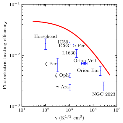
Figure 15: Photoelectric heating efficiency as a function of the ionization parameter $\gamma$. The data for the dense PDRs NGC 2023 and the Orion Bar is taken from Hollenbach & Tielens (1999), the data for the Horsehead and L1630 is from Pabst et al. (2017), the data for diffuse PDRs is from Gry et al. (1992) and van Dishoeck & Black (1986), and the data for IC59 and IC63 is from Andrews et al. (2018). The red line shows the model of Bakes & Tielens (1994). The error bars for $o$ Per, IC59 and IC63 have been omitted for clarity.

In the diffuse ISM most of the gas heating is through the photoelectric effect on polycyclic aromatic hydrocarbons (PAHs) and small dust grains (e.g., Wolfire et al. 1995). In this process, FUV ($6$ eV to $13.6$ eV) photons are absorbed by PAHs and very small dust grains causing them to eject electrons which then heat the gas through collisions. Our understanding of the ISM is intimately related to the efficiency of this process, as it couples the interstellar radiation field to the gas temperature. In general, the gas photoelectric heating efficiency $(\epsilon_{\mathrm{pe}}$) is less than $10\%$ (e.g., Bakes & Tielens 1994; Weingartner & Draine 2001) and most of the energy absorbed by the dust is re-radiated in the infrared (IR). Its exact value will depend on the charge state of the dust grains, and hence on the ionization parameter $\gamma=G_{0}T_{\mathrm{e}}^{1/2}n_{\mathrm{e}}^{-1}$ (e.g., Hollenbach & Tielens 1999). The gas heating efficiency through the photoelectric effect can be estimated as ([CII]+[OI])/TIR (e.g., Pabst et al. 2017), where TIR is the total infrared flux and [OI] is the gas cooling through the line of atomic oxygen at $63$ $\mu$m. Here we ignore the possible contribution from the [OI] line at $63$ $\mu$m to the gas cooling since for a gas density of $n_{\mathrm{H}}\approx 3\times 10^{3}$ cm^-3 it is estimated to be roughly $5\%$ of the total gas cooling (e.g., Tielens 2010). As a proxy for TIR we use the Lombardi et al. (2014) maps of dust properties. These present the properties of the dust spectral energy distribution derived from fitting a modified blackbody to continuum data in the wavelength range $100$ $\mu$m to $3000$ $\mu$m as observed by Herschel and Planck. From the maps of Lombardi et al. (2014) we can obtain the TIR flux by integrating the modified blackbody between the wavelength range $20$ $\mu$m to $1000$ $\mu$m. The median of the TIR flux over the $18\arcmin$ circle that contains the low-frequency radio continuum is $0.096$ erg s^-1 cm^-2 sr^-1. Then, if we correct for beam dilution, we have $\epsilon_{\mathrm{pe}}=(6.9\pm 0.3)\times 10^{-3}$. For $G_{0}$ we use a value of $550$, the mean of the values found by Abel et al. (2016) for components A and B of the Veil based on the properties of the Trapezium stars (Ferland et al. 2012) and their relative distances, $2$ pc and $4.2$ pc. This $G_{0}$ value should be valid for most of the gas in the Veil as this structure is a spherical shell (Pabst et al. 2019). Using this value of $G_{0}$ and the derived gas properties we have that $\gamma=(3\mbox{--}6)\times 10^{3}$ K^1/2 cm³. A comparison between the heating efficiency as a function of $\gamma$ measured towards different regions is presented in Figure 15. The overall picture is that the theoretical predictions of the heating efficiency overpredict the observed values. This discrepancy might mean that the heating efficiency is lower, that the PAH abundance is lower, or that there is a bias in the observed values due to the use of TIR as an estimate of the FUV radiation field (e.g., Hollenbach & Tielens 1999; Okada et al. 2013; Kapala et al. 2017). Here we do not investigate this further.

4.2 Background molecular cloud; Orion A

Here we use the C$30\alpha$, C$65\alpha$, C$91\alpha$, and $158$ $\mu$m-[CII] lines to study the gas properties in the dense PDR in the envelope of Orion A. Emission from these lines at a velocity of $\approx 9$ km s^-1 is associated with the background molecular cloud.

4.2.1 CRRLs

The C$30\alpha$ cube overlaps with the observations of C$65\alpha$ and C$91\alpha$ of Wyrowski et al. (1997) (see Figure 9). Here we use the ratios between the intensities of these lines to constrain the gas properties. Since the lines trace the PDR at the interface between the HII region and the background molecular cloud, the background continuum will be zero (e.g., Natta et al. 1994).

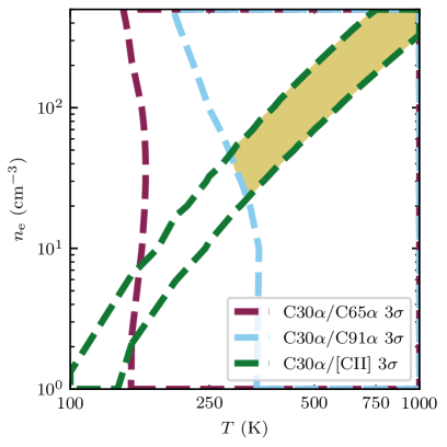
Figure 16: Constraints on the gas temperature and electron density imposed by the ratios between the C$30\alpha$, C$65\alpha$, C$91\alpha$ and $158$ $\mu$m-[CII] lines. The yellow shaded region shows where the constraints overlap.

We focus on a $40\arcsec$ region to the north of Orion-KL, at $(\alpha,\delta)_{\mathrm{J2000}}=(05^{\mathrm{h}}35^{\mathrm{m}}16.7828^{\mathrm{s}},-05\degr 22^{\mathrm{m}}02.7225^{\mathrm{s}})$. There the C$30\alpha$, C$65\alpha$, and C$91\alpha$ cubes overlap, and Wyrowski et al. (1997) provides measurements of the C$65\alpha$ and C$91\alpha$ intensity. We estimate the error on the intensity of the C$91\alpha$ line from the profile shown in Figure 2 of Wyrowski et al. (1997). The root mean square (rms) of the spectrum is close to $0.05$ K, and given that the line profile is narrow and shows little contribution from the HeRRL, we estimate an error of $0.1$ km s^-1 on the line width. These values imply a $1\sigma$ error of $0.2$ K km s^-1 for a $2.9$ K km s^-1 intensity. For the C$65\alpha$ line we adopt an error of $20\%$ of the observed line intensity. The C$30\alpha$ line intensity over this region is $71\pm 13$ mK km s^-1.

In the studied region, the C$30\alpha$/C$65\alpha$ line ratio is $0.12\pm 0.02$ and the C$30\alpha$/C$91\alpha$ line ratio $0.038\pm 0.005$. The constraints imposed on the gas temperature and density by these ratios are shown in Figure 16. The temperature is constrained to values higher than $150$ K, but they do not constrain the electron density. The C$65\alpha$/C$91\alpha$ line ratio is $0.30\pm 0.06$, and, given the adopted errors, it does not constrain the gas properties.

To fully exploit the power of CRRLs, to provide independent constraints on the gas properties, higher signal-to-noise detections of the observed lines are required. For example, if the error on the intensity of the C$65\alpha$ line was $10\%$ of the observed value and that of the C$30\alpha$ a factor of two lower, then it would be possible to determine the gas temperature and density using only CRRLs. Under this assumption, the gas temperature would be constrained to within $10$ K and the electron density within $45$ cm^-3. Alternatively, we could use CRRLs at lower frequencies. At lower frequencies the frequency separation between adjacent C$n\alpha$ lines decreases, hence it becomes easier to achieve higher signal-to-noise ratios by stacking. Higher resolution observations are also important as they make it possible to observe the layered structure on higher density PDRs.

4.2.2 CRRLs and FIR [CII] line

When the $158$ $\mu$m-[CII] line is optically thick its ratio relative to a CRRL depends on the C⁺ column density, and thus we need an independent measure of the column density to compare them. To determine the C⁺ column density we use the [¹³CII] $F=2\mbox{--}1$ line. This line has a velocity difference of $11.2$ km s^-1 with respect to the $158$ $\mu$m-[CII] line. To estimate the column density from $158$ $\mu$m-[CII] and its isotopologue we follow the analysis of Goicoechea et al. (2015). We adopt the corrected line strengths of Ossenkopf et al. (2013) for the three [¹³CII] hyperfine structure lines and a [C/¹³C] abundance ratio of $67$ (Langer & Penzias 1990), and compute the excitation temperature assuming that the $158$ $\mu$m-[CII] line is optically thick.

For the region studied previously in CRRLs ($(\alpha,\delta)_{\mathrm{J2000}}$ $=(05^{\mathrm{h}}35^{\mathrm{m}}16.7828^{\mathrm{s}},-05^{\mathrm{\circ}}22^{\mathrm{m}}02.7225^{\mathrm{s}})$), we have peak line temperatures of $177$ K and $4$ K for [CII] and [¹³CII] $F=2\mbox{--}1$, respectively. This translates to an optical depth of $2.3$. For a background temperature of $35$ K, the excitation temperature of the $158$ $\mu$m-[CII] line is $230$ K. Using the observed full width at half maximum of $\approx 4$ km s^-1 this corresponds to a [CII] column density of $9.7\times 10^{18}$ cm^-2.

With an estimate of the [CII] column density we can use the ratio between the $158$ $\mu$m-[CII] line and the CRRLs to further constrain the gas properties. For the C$30\alpha/$[CII] ratio we have a value of $(1.4\pm 0.2)\times 10^{-4}$. The C$30\alpha/$[CII] ratio puts a constraint on the gas properties of the form $n_{\mathrm{e}}\propto T^{3}$, shown in Figure 16 with green dashed lines. Using the lower frequency CRRLs or the [¹³CII] $F=2\mbox{--}1$ line results in a similar constraint.

4.2.3 Combined constraints

As seen in Figure 16 the constraints imposed by the CRRL and $158$ $\mu$m-[CII] line ratios overlap for temperatures higher than $300$ K and an electron density higher than $25$ cm^-3. If we assume that all the free electrons come from the ionization of carbon, and a carbon abundance with respect to hydrogen of $1.4\times 10^{-4}$, this sets a lower limit to the gas thermal pressure of $5\times 10^{7}$ K cm^-3. This is similar to the thermal pressure for the atomic gas layers found by Goicoechea et al. (2016) towards the Orion Bar.

4.2.4 PDR models

Motivated by the resemblance between the observed gas distribution (Figure 11) and the structure seen in a PDR (Figure 12), we compare the observed line intensities to the predictions of PDR models. In a PDR close to face-on the C⁺ column density is determined by the radiation field and gas density, hence we do not need an independent estimate of the column density. The PDR models also take into account the gas density and temperature structure.

We focus on the region previously studied in Sect. 4.2.1, towards the north of Orion-KL. To make a comparison with the PDR model predictions, we need to take into account the geometry; if the PDRs are not observed face-on, then the column density along the line of sight is not determined by the radiation field and density. For example, the Orion Bar has a length of $0.28\pm 0.06$ pc along the line of sight (Salgado et al. 2016), while in the perpendicular direction its extent is $\approx 0.02$ pc (e.g., Wyrowski et al. 1997; Goicoechea et al. 2016). To determine the length of the PDR along the line of sight we use the intensity of the C$30\alpha$ line, then we use this to scale the rest of the line intensities. Once we have scaled the line intensities, we determine which models are able to reproduce the observed line intensities and ratios.

First we make a comparison with constant density PDR models. These models require densities higher than $5\times 10^{5}$ cm^-3 to explain the line intensities and ratios. This is equivalent to an electron density higher than $70$ cm^-3, which is consistent with the values found towards this region (Figure 16); however, these models also require radiation fields $G_{0}\geq 5\times 10^{5}$. In this region, which is a factor of $2.5$ closer to the Trapezium than the Orion Bar, the incident radiation field should be a factor of six larger than in the Bar, or $G_{0}\approx 1.4\times 10^{5}$. This shows that constant density PDR models are not able to explain the observed line properties given reasonable input parameters.

Next we make a comparison with stationary isobaric PDR models. In this case the models require thermal pressures larger than $5\times 10^{7}$ K cm^-3, and a radiation field $G_{0}=(0.4\mbox{--}1)\times 10^{5}$ to explain the observations. The isobaric model that best reproduces the observations has $G_{0}=1\times 10^{5}$ and $P_{\mathrm{th}}=5\times 10^{7}$ K cm^-3. In this case the radiation field and gas thermal pressure are consistent with independent estimates. Stationary isobaric PDR models also provide better results when explaining observations of excited molecular tracers (e.g., Joblin et al. 2018).

Given the best fit isobaric PDR model, we assess whether the constraints derived assuming a homogeneous gas slab are reasonable. In this model the CRRL emission originates mostly from a layer with a gas temperature of $200$ K, and a similar excitation temperature for the $158$ $\mu$m-[CII] line. The gas temperature is $30\%$ lower than that derived under the homogeneous slab model ($300$ K). The electron density in the isobaric PDR model is $75$ cm^-3 in the layer where the CRRL emission peaks, i.e., roughly $50\%$ higher than in the homogeneous slab model. Therefore, the lower limits from the homogeneous model predict a gas thermal pressure which is $25\%$ to $50\%$ lower than that predicted by a stationary isobaric PDR model. This difference is not significant considering that the isobaric PDR models used only sparsely sample the $P_{\mathrm{th}}$–$G_{0}$ space.

5 Summary

We presented CRRL observations towards Orion A in the frequency range $230$–$0.15$ GHz, including the first detections of the lines in absorption, with the aim of comparing them with the $158$ $\mu$m-[CII] line. The CRRLs towards Orion A show the presence of multiple velocity components, similar to what is observed through other tracers of neutral gas (e.g., the $21$ cm-HI line or the $158$ $\mu$m-[CII] line). We identify CRRL emission associated with the Veil and the background molecular cloud.

We find that the Veil is preferentially traced using lines at frequencies $\lesssim 2$ GHz ($n>150$ for C$n\alpha$ lines), similar to the findings of previous studies, because M42 becomes opaque at these frequencies and its continuum produces significant amplification of the foreground lines. Using C$280\alpha$/C$351\alpha$ and C$350\alpha$/[CII] line ratios we were able to constrain the properties of the Veil on $36\arcmin$ scales ($4.3$ pc). We find a gas temperature of $30$ K$\leq T_{\mathrm{e}}\leq 45$ K and an electron density of $0.65$ cm${}^{-3}\leq n_{\mathrm{e}}\leq 0.95$ cm^-3, where the quoted ranges consider $3\sigma$ errors on the line ratios. From these physical conditions we constrain the gas cooling rate through the $158$ $\mu$m-[CII] line and the efficiency of photoelectric heating. We find a lower limit on the gas cooling rate of $(4\pm 0.2)\times 10^{-26}$ erg s^-1 (H-atom)^-1, and a photoelectric heating efficiency of $\epsilon_{\mathrm{pe}}=(6.9\pm 0.3)\times 10^{-3}$ for $\gamma=(3\mbox{--}6)\times 10^{3}$ K^1/2 cm³. Based on these values, the Veil is classified somewhere between a diffuse cloud and a dense PDR.

The dense PDR, at the interface between the HII region and Orion A, is traced using CRRLs at frequencies $\gtrsim 2$ GHz. By comparing the spatial distribution of the C$30\alpha$ and C$65\alpha$ lines to that of the $158$ $\mu$m-[CII] and ¹²CO$(2\mbox{--}1)$ lines, we find a clump to the south of the Trapezium where we can observe the layered PDR structure. The relative location of the C$65\alpha$ line with respect to the $158$ $\mu$m-[CII] line indicates that in a dense PDR the radio lines trace colder gas than the FIR line.

Motivated by the observed distribution of atomic and molecular gas tracers we compared the intensity of the CRRLs and the $158$ $\mu$m-[CII] line to the predictions of PDR models. We find that stationary isobaric PDR models are able to reproduce the observations. They imply a thermal gas pressure $\geq 5\times 10^{7}$ K cm^-3, and likely a factor of two higher. This result agrees with the thermal pressure derived from CRRL and $158$ $\mu$m-[CII] line ratios.

This work shows that the combined use of CRRLs and the $158$ $\mu$m-[CII] line is a powerful tool for studying the ISM. They provide an alternative method to determine the gas physical conditions (temperature and electron density). The physical conditions derived this way can be combined with the information provided by the $158$ $\mu$m-[CII] line to determine the gas heating and cooling.

With new and upgraded telescopes (e.g., SKA, ngVLA, uGMRT, LOFAR2.0), CRRLs will allow us to explore the ISM in our Galaxy and others (Morabito et al. 2014; Emig et al. 2018). In distant galaxies, where spectral tracers of the ISM may be harder to come by, the use of CRRLs and the $158$ $\mu$m-[CII] line can provide important constraints on the properties of the ISM across cosmic time. Our work shows how these constraints can be obtained by taking into consideration the structure of a PDR.

Appendix A Nonlinear gain correction

Under ideal circumstances, the relation between the raw counts measured by a radio telescope $P$, the source temperature $T_{\mathrm{sou}}$, and the system temperature $T_{\mathrm{sys}}$ will be of the form

$$P^{\mathrm{[CAL]}}=G(T_{\mathrm{sou}}+T_{\mathrm{sys}}^{\mathrm{[CAL]}})+C,$$ (3)

where $G$ is the conversion factor between temperature and telescope units (counts) and $C$ a constant offset between the two scales. Here we adopted the nomenclature of Winkel et al. (2012), in which $T_{\mathrm{sys}}^{\mathrm{[CAL]}}$ denotes the system temperature, considering the possible contribution from a calibration signal $T_{\mathrm{cal}}$, and $T_{\mathrm{sou}}$ is the temperature of the astronomical source of interest which includes both continuum and line, $T_{\mathrm{cont}}$ and $T_{\ell}$, respectively. In order to determine the conversion between counts and temperature, procedures such as those outlined in Winkel et al. (2012) were used.

Given the nature of the signal path on a radio telescope, it is possible that relation 3 will break down. This could be due to the amplifiers being driven out of their linear response regime (e.g., if a bright source is observed). This has the effect of changing Equation 3 to

$$P^{\mathrm{[CAL]}}=G(T_{\mathrm{sou}}+T_{\mathrm{sys}}^{\mathrm{[CAL]}})+G_{\mathrm{nl}}(T_{\mathrm{sou}}+T_{\mathrm{sys}}^{\mathrm{[CAL]}})^{2}+C.$$ (4)

Here, $G_{\mathrm{nl}}$ represents the nonlinear contribution of the amplifier gain.

If Equation 3 is no longer valid, and we can represent the conversion between raw counts and temperature using Equation 4, then it is possible to calibrate the raw counts if we make some assumptions about $T_{\mathrm{sou}}$. To estimate $G_{\mathrm{nl}}$ we can use a reference position $P_{\mathrm{ref}}$, ideally devoid of any astronomical signal, and a model of $T_{\mathrm{sou}}$. Then,

$$G_{\mathrm{nl}}=\frac{P_{\mathrm{sou}}-P_{\mathrm{ref}}-GT_{\mathrm{sou}}}{2T_{\mathrm{sys}}+T_{\mathrm{sou}}^{2}}$$ (5)

If we are interested in recovering the temperature of a spectral line, we can work with the continuum subtracted spectra $P_{\ell}^{\mathrm{[CAL]}}=P^{\mathrm{[CAL]}}-P_{\mathrm{cont}}^{\mathrm{[CAL]}}$. The continuum $P_{\mathrm{cont}}^{\mathrm{[CAL]}}$ can be estimated from line-free channels. The line brightness temperature $T_{\ell}$ is then obtained from

$$T_{\ell}=P_{\ell}^{\mathrm{[CAL]}}\left[G+G_{\mathrm{nl}}(T_{\ell}+2T_{\mathrm{cont}}+2T_{\mathrm{sys}}^{\mathrm{[CAL]}})\right]^{-1}$$ (6)

Appendix B Gaussian fits to RRL spectra

A decomposition of the spectra presented in Figure 4 into Gaussian components is tabulated in Table 4.

Table 4: Best fit Gaussian parameters for RRLs observed towards M42

Region	$v_{\mathrm{lsr}}$	$T_{\mathrm{mb}}$	$\Delta v$
	(km s-1)	(K)	(km s-1)
H$137\alpha$	$-6.92\pm 0.05$	$3.95\pm 0.01$	$32.9\pm 0.1$
H$145\alpha$	$-7.57\pm 0.08$	$2.98\pm 0.01$	$34.7\pm 0.2$
H$151\alpha$	$-8.5\pm 0.1$	$4.40\pm 0.03$	$34.8\pm 0.3$
H$155\alpha$	$-8.2\pm 0.1$	$2.21\pm 0.01$	$36.0\pm 0.2$
H$156\alpha$	$-7.8\pm 0.1$	$2.85\pm 0.02$	$36.1\pm 0.3$
H$164\alpha$	$-7.9\pm 0.1$	$2.26\pm 0.02$	$36.0\pm 0.4$
H$174\alpha$	$-8.3\pm 0.2$	$1.56\pm 0.02$	$37.0\pm 0.5$
H$280\alpha$	$0\pm 2$	$0.010\pm 0.002$	$25\pm 5$
He$137\alpha$	$-5\pm 1$	$0.42\pm 0.02$	$31\pm 2$
He$145\alpha$	$-11\pm 2$	$0.25\pm 0.04$	$23\pm 3$
He$151\alpha$	$-6\pm 1$	$0.40\pm 0.05$	$15\pm 4$
He$155\alpha$	$-10\pm 3$	$0.17\pm 0.02$	$24\pm 5$
He$156\alpha$	$-7\pm 5$	$0.15\pm 0.04$	$16\pm 10$
He$164\alpha$	$-7\pm 3$	$0.20\pm 0.03$	$17\pm 6$
He$174\alpha$	$-14\pm 2$	$0.19\pm 0.03$	$32\pm 4$
C$137\alpha$	$7.3\pm 0.6$	$0.26\pm 0.05$	$12\pm 2$
C$145\alpha$	$6.3\pm 0.7$	$0.24\pm 0.06$	$9\pm 2$
C$151\alpha$	$5.2\pm 0.8$	$0.67\pm 0.07$	$10\pm 1$
C$155\alpha$	$4.4\pm 0.4$	$0.31\pm 0.06$	$9\pm 1$
C$156\alpha$	$6\pm 1$	$0.5\pm 0.1$	$10\pm 1$
C$164\alpha$	$4.9\pm 0.7$	$0.54\pm 0.07$	$10\pm 1$
C$174\alpha$	$5.1\pm 0.3$	$0.47\pm 0.05$	$6\pm 1$
C$280\alpha$	$0.7\pm 1.0$	$-0.023\pm 0.003$	$11\pm 1$