Variational training of neural network approximations of solution maps for physical models

Abstract

A novel solve-training framework is proposed to train neural network in representing low dimensional solution maps of physical models. Solve-training framework uses the neural network as the ansatz of the solution map and trains the network variationally via loss functions from the underlying physical models. Solve-training framework avoids expensive data preparation in the traditional supervised training procedure, which prepares labels for input data, and still achieves effective representation of the solution map adapted to the input data distribution. The efficiency of solve-training framework is demonstrated through obtaining solution maps for linear and nonlinear elliptic equations, and maps from potentials to ground states of linear and nonlinear Schrödinger equations.

Keywords. Neural network; solution map for PDEs; fast algorithm; hierarchical matrix; unsupervised training.

1 Introduction

Simulation of physical models has been one of main driven forces for scientific computing. Physical phenomena at different scales, e.g., macroscopic scale, microscopic scale, etc., are characterized by Newton’s laws of motion, Darcy’s law, Maxwell’s equations, Schrödinger equation, etc. Solving these equations efficiently, especially those nonlinear ones, has challenged computational scientists for decades and led to remarkable development in algorithms and in computing hardware. As the rise of machine learning, particularly deep learning, many researchers have been attempting to adopt artificial neural networks (NN) to represent the high-dimensional solutions or the low-dimensional solution maps. This paper proposes a variational training framework for solving the solution map of low-dimensional physical models via NNs. Here we emphasize solving a solution map in contrast with fitting a solution map, where solving can be to some extent viewed as unsupervised learning with input functions only and fitting refers to supervised learning with both input functions and the corresponding solutions.

Solving the solution map for physical models is feasible due to an intrinsic difference between the physical problems and other data-driven problems, e.g., handwriting recognition, speech recognition, spam detection, etc. Indeed, for physical models, the solution maps are governed by well-received equations, which are often expressed in partial differential equations (PDEs), whereas the conventional machine learning tasks such as image classification rely on human labeled data set without explicit expression for the underlying model. Benefiting from such a difference, we design loss functions based on the PDEs, in another word, we adopt the model information into the loss functions, and solve the solution map directly without knowing solution functions.

1.1 Related work

A number of recent work utilized NNs to address physical models. Generally, they can be organized into three groups: representing solutions via NNs, representing solution maps via NNs, and optimizing traditional iterative solvers via NNs. Representing solutions of physical models, especially high-dimensional ones, has been a long-standing computational challenge. NN with multiple input and single output can be used as an ansatz for the solutions of physical models or PDEs, which is first explored in [29] for low-dimensional solutions. Many high-dimensional problems, e.g., interacting spin models, high-dimensional committor functions, etc., have been recently considered for solutions using NN ansatz with variants optimization strategies [5, 7, 9, 19, 26, 37, 36]. NN, in this case, is valuable in its flexibility and richness in representing high-dimensional functions.

Representing the solution map of a nonlinear problem is challenging as well. For linear problems, the solution map can be represented by a simple matrix (i.e., Green’s function for PDE problems). While the efficient representation for solution map is unknown for most nonlinear problems. Traditional methods in turn solve nonlinear problem via iterative methods, e.g., fixed point iteration. Since NN is able to represent high dimensional nonlinear mappings, it has also been explored in recent literature to represent solution maps of low-dimensional problems on mesh grid, see e.g, [10, 11, 12, 20, 25, 27, 30, 34, 38, 39]. These NNs are fitted by a set of training data with solution ready, i.e., labeled data. Most works from the first two groups focus on creative design of NN architectures, in particular trying to incorporate knowledge of the PDE into the representation.

The last group, very different from previous two, adopts NN to optimize traditional iterative methods [14, 23, 24, 35]. Once the iterative methods are optimized on a set of problems, generalization to different boundary conditions, domain geometries, and other similar models, is explored and can be sometimes guaranteed [23].

1.2 Main Idea

The goal of this work is to propose a new paradigm of training neural networks to approximate solution maps for physical PDE models, which does not rely on existing PDE solvers or collected solution data. The main advantages come in two folds: the new training framework removes the expensive data preparation cost and obtains an input-data-adaptive NN with better accuracy in terms of intrinsic criteria from the PDE after training.

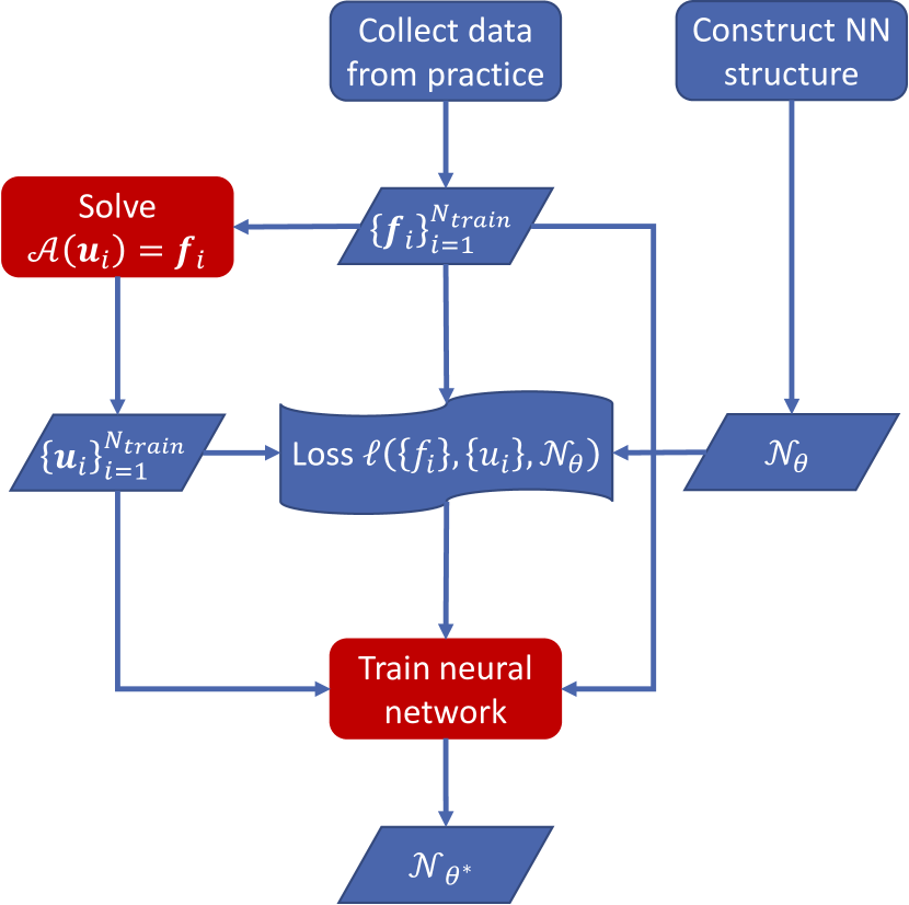
(a) Fit-training framework.

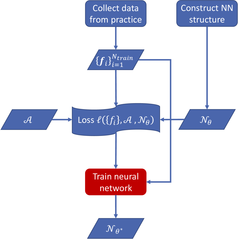
(b) Solve-training framework.

Figure 1: Flowchart of (a) fit-training framework and (b) solve-training framework. Rounded corner rectangles in general indicate processes whereas the red ones are computationally expensive processes; parallelograms indicate data or NNs; punched tapes are loss functions which require creative design depending on the problem; line arrows indicate dependencies between blocks.

We now explain the main idea of the new training framework through the example of solving a (possibly nonlinear) system of equations. Later in Section 3, we will show that the training framework can be applied to solve the solution map of linear and nonlinear eigenvalue problem as well.

Let us consider a system of equations, written as

$$\mathcal{A}(\bm{u})=\bm{f},$$ (1)

with $\bm{u}$ and $\bm{f}$ denoting solution and input functions on a mesh and $\mathcal{A}$ denoting a discretized forward operator. The goal here is to obtain the solution map, i.e.,

$$\bm{u}=\mathcal{A}^{-1}(\bm{f})\approx\mathcal{N}_{\theta}(\bm{f}),$$ (2)

which is approximated by a NN $\mathcal{N}_{\theta}$ parameterized by $\theta$. The input data $\bm{f}$ is usually collected from practice following an unknown distribution $\mathcal{D}_{f}$, denoted as $\bm{f}\sim\mathcal{D}_{f}$. Ideally, NN not only approximates the inverse map $\mathcal{A}^{-1}$, but also adapts to the distribution, i.e., $\mathcal{N}_{\theta}\approx\mathcal{A}^{-1}\mid_{\mathcal{D}_{f}}$.

Almost all previous works design NN $\mathcal{N}_{\theta}$ based on properties of the problem and then fit the solution map following the flowchart in Figure 1 (a). We call such a training procedure fit-training framework. In practice, there are two procedures for generating training data pair, $\{\bm{u}_{i},\bm{f}_{i}\}_{i=1}^{N_{\text{train}}}$

1. Collect a set of $\{f_{i}\}_{i=1}^{N_{\text{train}}}$ and solve $\bm{u}_{i}=\mathcal{A}^{-1}(\bm{f}_{i})$ with traditional methods;

2. Randomly generate a set of solution data, $\{\bm{u}_{i}\}_{i=1}^{N_{\text{train}}}$ and evaluate $\bm{f}_{i}=\mathcal{A}(\bm{u}_{i})$.

The first procedure suffers from expensive traditional method in solving $\mathcal{A}^{-1}$, especially when the equation is complicated and nonlinear. While, the resulting training data set from the first procedure follows the practical distribution $\mathcal{D}_{f}$. Hence fitting $\mathcal{N}_{\theta}$ with this data set approximates $\mathcal{A}^{-1}\mid_{\mathcal{D}_{f}}$. The second procedure is efficient in generating data since $\mathcal{A}$ is usually cheap to evaluate. However, the data set lacks proper distribution, i.e., $\bm{f}_{i}\not\sim\mathcal{D}_{f}$. An accurate solution map requires $\mathcal{N}_{\theta}$ to be a good representation of $\mathcal{A}^{-1}$ instead of $\mathcal{A}^{-1}\mid_{\mathcal{D}_{f}}$, which is much more difficult to approximate in general.

Under our new training framework, illustrated in Figure 1 (b), $\bm{u}_{i}$ is not required in the loss function hence not required in the training procedure. Instead, the forward mapping $\mathcal{A}$ is brought into the loss function. One simplest example of such a loss function in the sense of mean square error is

$$\ell\Big{(}\{\bm{f}_{i}\}_{i=1}^{N_{\text{train}}},\mathcal{A},\mathcal{N}_{\theta}\Big{)}=\frac{1}{N_{\text{train}}}\sum_{i=1}^{N_{\text{train}}}\norm{\bm{f}_{i}-\mathcal{A}\big{(}\mathcal{N}_{\theta}(\bm{f}_{i})\big{)}}^{2},$$ (3)

where $\mathcal{A}$ in our implementation is represented by an NN with fixed parameters. In contrast to the fit-training framework, the proposed training framework – solve-training framework – has at least three advantages:

1. Solving $\bm{u}_{i}=\mathcal{A}^{-1}(\bm{f}_{i})$ via expensive traditional method is not needed;

2. The trained NN $\mathcal{N}_{\theta}$ is able to capture $\mathcal{A}^{-1}\mid_{\mathcal{D}_{f}}$;

3. The parameters obtained through solve-training framework minimizes the “$\mathcal{A}$-norm” between $\mathcal{N}_{\theta}(\bm{f})$ and $\bm{u}_{*}=\mathcal{A}^{-1}(\bm{f})$, i.e.,

   $$\norm{\bm{f}-\mathcal{A}\big{(}\mathcal{N}_{\theta}(\bm{f})\big{)}}=\norm{\bm{u}_{*}-\mathcal{N}_{\theta}(f)}_{\mathcal{A}},$$ (4)

   if $\mathcal{A}$ satisfies assumptions such that $\norm{\cdot}_{\mathcal{A}}$ is well-defined.

Regarding the last point above, fit-training framework minimizes 2-norm between $\mathcal{N}_{\theta}(\bm{f})$ and $\bm{u}_{*}$, which corresponds to least square fitting for linear operators. Hence we claim that solve-training framework is more likely to obtain an NN $\mathcal{N}_{\theta}$ which solves $\mathcal{A}(\bm{u})=\bm{f}$ given $\bm{f}\sim\mathcal{D}_{f}$. Other than the neural network approximation error, solve-training framework contains one more source of approximation, the discretization error of the real forward operator to $\mathcal{A}$. Since the discretized forward map $\mathcal{A}$ is represented by a fixed neural network, which does not increase the number of trainable parameters in the training part, we can use high-accuracy discretization schemes to significantly reduce the discretization error and make the error much less than the neural network approximation error. The discretization error is also contained in the fit-training framework, since we need to solve the discretized equation to provide training data.

In this work, we demonstrate the power of the solve-training framework through training the NNs representing the solution maps of linear and nonlinear systems and linear and nonlinear eigenvalue problems. We remark that while finishing the work, we discovered some very recent works [3, 42] aiming at solving inverse problems, whose training strategy shares some similarity with the solve-training framework we proposed above.

1.3 Organization

The rest of the paper is organized as the following. Section 2 applies the solve-training framework to solving linear and nonlinear systems. The corresponding numerical results are attached right after the problem description. Similar structure applies to Section 3, in which we solve linear and nonlinear eigenvalue problems rising from Schrödinger equations. Finally, Section 4 concludes the paper with discussions on extensibility.

2 Solving linear and nonlinear systems

This section aims to show that the solve-training framework can be applied to obtain the NN representation of the solution maps of linear and nonlinear systems. The main idea of solve-training framework for solving systems has been illustrated in Section 1.2. We will demonstrate the efficiency of the solve-training framework through two examples, linear elliptic equation and nonlinear elliptic equation.

2.1 Linear elliptic equations

In this section, we focus on the two dimensional linear variable coefficient elliptic equations with periodic boundary condition, i.e.,

$$-\nabla\cdot a(x,y)\nabla u(x,y)=f(x,y),\quad(x,y)\in\Omega=[0,1)^{2},$$ (5)

where $a(x,y)>0$ denote variable coefficients. Such an equation appears in a wide range of physical models governed by Laplace’s equation, Stokes equation, etc. For (5) with constant coefficients, the inverse operator  has an explicit Green’s function representation and can be applied efficiently with quasilinear cost through fast multipole methods [13, 15, 41], or other related fast algorithms [8, 22]. When the coefficient is variable, then the operator in (5) is discretized into a sparse matrix, and solved via iterative methods with efficient preconditioners [6, 16, 18, 21, 31, 40]. Among these preconditioners, $\mathcal{H}$-matrices [16, 18] are efficient preconditioners of simplest algebraic form and the structures with modifications are recently extended to NN structures [10, 11]. While, the construction of the $\mathcal{H}$-matrices for the inverse of variable coefficient elliptic equations requires sophisticated matrix-vector multiplication on structured random vectors [33]. In this section, we adopt the original structure of $\mathcal{H}$-matrix in $\mathcal{N}_{\theta}$ with and without ReLU layers. Solve-training framework then provides a method to construct the $\mathcal{H}$-matrix with a limited number of input functions.

The discretization of (5) used here is the five-point stencil on a $64\times 64$ uniform grid. The discretization points are $\{x_{i},y_{j}\}_{i,j=0}^{63}$ with $x_{i}=i/64$ and $y_{j}=j/64$. And the discrete variable coefficient $a(x_{i},y_{j})$ is a Chess board field as,

$$a(x_{i},y_{i})=\begin{cases}10,&{\lfloor\frac{i+j}{8}\rfloor}\equiv 0\,(\mathrm{mod}\,2)\\ 1,&{\lfloor\frac{i+j}{8}\rfloor}\equiv 1\,(\mathrm{mod}\,2)\\ \end{cases}.$$ (6)

And we generate $N_{\text{train}}$ random vectors $\{\bm{f}_{i}\}_{i=1}^{N_{\text{train}}}$ as the training data. Each $\bm{f}_{i}$ is a vector of length $64^{2}$ with each entry being uniform random on $\Big{[}-\sqrt{3/64^{2}},\sqrt{3/64^{2}}\Big{]}$ such that $\mathbb{E}\Big{(}\norm{\bm{f}_{i}}\Big{)}=1$  and subtract its mean to incorporate with the periodic boundary condition. This procedure defines $\mathcal{D}_{f}$, which will be less emphasized for linear model in this section. Another set of $N_{\text{test}}=5,000$ random vectors of the same distribution, $\{\bm{g}_{i}\}_{i=1}^{N_{\text{test}}}$, is generated for testing purpose. The reported relative error is calculated as follows,

$$\frac{1}{N_{\text{test}}}\sum_{i=1}^{N_{\text{test}}}\frac{\norm{\bm{g}_{i}-\mathcal{A}\Big{(}\mathcal{N}_{\theta}(\bm{g}_{i})\Big{)}}}{\norm{\bm{g}_{i}}}.$$ (7)

Four $\mathcal{H}$-matrices are generated and compared in this section. The structures of all these $\mathcal{H}$-matrices are generated from bi-partition of the domain up to four layers and each low-rank submatrix is of rank 96. Readers are referred to the textbook [17] for the detailed structure of an $\mathcal{H}$-matrix. The first $\mathcal{H}$-matrix is constructed directly from the inversion of the discretized sparse matrix and each low-rank block is constructed via the truncated singular value decomposition (SVD). This $\mathcal{H}$-matrix is close-to-optimal in the standard $\mathcal{H}$-matrix literature and is used as the baseline for the comparison. We denote it as $\mathcal{H}$-matrix (SVD) in the later content. The second and third $\mathcal{H}$-matrices are constructed in the same way in Tensorflow [1]. The second one is initialized with random coefficients and then trained, whereas the third one is initialized with the baseline $\mathcal{H}$-matrix and then trained. They are denoted as NN-$\mathcal{H}$-matrix (rand init) and NN-$\mathcal{H}$-matrix (SVD init) respectively. The last $\mathcal{H}$-matrix uses the same structure but with each small dense block coupled with $5$ ReLU layers in the similar fashion as in [11]. This $\mathcal{H}$-matrix is initialized with SVD coefficients and the ReLU part is initialized in a way such that the initial output (no train) is the same as that of $\mathcal{H}$-matrix (SVD) and then trained. It is denoted as NLNN-$\mathcal{H}$-matrix (SVD init).

We train the later three $\mathcal{H}$-matrices under the solve-training framework with Adam optimizer [28]. The batch size is 100 for all trainings. For NN-$\mathcal{H}$-matrix (SVD init) and NLNN-$\mathcal{H}$-matrix (SVD init), a fixed stepsize $2\times 10^{-6}$ is used. While, for NN-$\mathcal{H}$-matrix (rand init), the stepsize is initialized as $2\times 10^{-4}$ following a steady exponential decay to $2\times 10^{-6}$. For each $\mathcal{H}$-matrix, we train the NN for three times and report the best among them. Default values are used for all other unspecified hyperparameters.

Numerical Results

We first compare the performance of the first three $\mathcal{H}$-matrices described above through numerical experiments under the solve-training framework.

$\mathcal{H}$-matrix	# Epoch	Train loss	Test loss	Train rel err	Test rel err
$\mathcal{H}$-matrix (SVD)	0	2.21e-3	2.20e-3	4.68e-2	4.66e-2
NN-$\mathcal{H}$-matrix (rand init)	25000	2.09e-4	3.38e-4	1.44e-2	1.83e-2
NN-$\mathcal{H}$-matrix (SVD init)	2000	2.43e-4	3.40e-4	1.55e-2	1.83e-2

Table 1: Train and test relative error of solve-training framework in linear elliptic equation for different $\mathcal{H}$-matrices. The train and test data sets are of size $N_{\text{train}}=10000$ and $N_{\text{test}}=5000$.

$\mathcal{H}$-matrix	# Epoch	Train loss	Test loss	Train rel err	Test rel err
$\mathcal{H}$-matrix (SVD)	0	2.20e-3	2.20e-3	4.66e-2	4.66e-2
NN-$\mathcal{H}$-matrix (rand init)	60000	1.34e-4	4.18e-2	1.15e-2	1.96e-1
NN-$\mathcal{H}$-matrix (SVD init)	6000	1.58e-4	7.20e-4	1.25e-2	2.67e-2

Table 2: Train and test relative error of solve-training framework in linear elliptic equation for different $\mathcal{H}$-matrices. The train and test data sets are of size $N_{\text{train}}=4000$ and $N_{\text{test}}=5000$.

(a)

(b)

Figure 2: Examples of residual of using the conjugate gradient method to solve the linear elliptic equation, where $\mathcal{H}$-matrix (SVD) and the trained NN-$\mathcal{H}$-matrix (SVD init) are applied as preconditioners respectively. The train and test data sets are of size $N_{\text{train}}=10000$ and $N_{\text{test}}=5000$.

Figure 3: The test relative error of NN-$\mathcal{H}$-matrix (SVD init) against epochs.

Table 1 and Table 2 present the number of epoches, train loss, test loss, train relative error, and test relative error for the first three $\mathcal{H}$-matrices with $N_{\text{train}}=10000$ and $N_{\text{train}}=4000$ respectively. All of these matrices share exactly the same structure and are all linear operators. Since these $\mathcal{H}$-matrices are trained on a uniform random input function and they are linear, the test relative error is generalizable to other non-normalized general input functions. When $N_{\text{train}}=10000$, we notice that NN-$\mathcal{H}$-matrix (rand init) and NN-$\mathcal{H}$-matrix (SVD init) achieve almost identical losses and relative errors after training under the solve-training framework, although the efficient training of NN-$\mathcal{H}$-matrix (rand init) requires more aggressive choice of stepsize in the beginning of the training. Since we inject part of the information of the system into the NN through the carefully designed architecture, training under solve-training framework is able to approximate the solution map with the number of training data $N_{\text{train}}$ smaller than the size of the matrix, i.e., $N_{\text{train}}=4000$. In this case, NN-$\mathcal{H}$-matrix (SVD init) is able to achieve similar results as that with $N_{\text{train}}=10000$. While NN-$\mathcal{H}$-matrix (rand init) achieves similar train results but less accurate test results.

In general, after training, the relative error for NN-$\mathcal{H}$-matrices is better than that of the $\mathcal{H}$-matrix (SVD), which means that the low-rank approximation in $\mathcal{H}$-matrix can be further improved. Low-rank approximation through truncated SVD achieves best 2/F-norm approximation locally in each block, whereas the trained NN-$\mathcal{H}$-matrix achieves near-optimal low-rank approximation in the global sense. Also, Figure 2 shows examples of residual of using the conjugate gradient method to solve the linear elliptic equation, where $\mathcal{H}$-matrix (SVD) and the trained NN-$\mathcal{H}$-matrix (SVD init) are applied as preconditioners respectively. The trained NN-$\mathcal{H}$-matrix achieves smaller residual than $\mathcal{H}$-matrix after the same number of iteration steps. Hence the solve-training framework can be applied to, either obtaining the $\mathcal{H}$-matrix representation of the inverse variable coefficient elliptic operator, or further refine some existing fast algorithms and achieves better approximation accuracy. In addition, Figure 3 shows the refinement step is quite efficient. The initial test relative error equals $0.0466$ and monotonically drops as the training goes on. After roughly $1000$ epoches, training with $N_{\text{train}}=10000$ samples, the test relative error reaches a plateau with values about $0.02$.

(a)

(b)

Figure 4: Train loss and test loss for (a) NN-$\mathcal{H}$-matrix (SVD init) and (b) NLNN-$\mathcal{H}$-matrix (SVD init) against epochs.

NLNN-$\mathcal{H}$-matrix (SVD init) is a nonlinear operator approximating the discrete inverse matrix of (5). Figure 4 (b) shows that its training behavior and as a comparison, Figure 4 (a) shows the training behavior of NN-$\mathcal{H}$-matrix (SVD init). We observe severe over fitting issue occurs in training NLNN-$\mathcal{H}$-matrix (SVD init). Hence, for linear elliptic equations, training linear operators under the solve-training framework is a more preferred strategy to represent $\mathcal{A}^{-1}\mid_{\mathcal{D}_{f}}$ accurately.

2.2 Nonlinear elliptic equation

In this section, we focus on a two dimensional nonlinear variable coefficient elliptic equation with periodic boundary condition, i.e.,

$$-\nabla\cdot a(x,y)\nabla u(x,y)+bu^{3}(x,y)=f(x,y),\quad(x,y)\in\Omega=[0,1)^{2},$$ (8)

where $a(x,y)>0$ denote variable coefficients and $b$ denotes the strength of the nonlinearity. This equation adds a cubic nonlinear term to (5) with coefficient $b$ and is also related to the nonlinear Schördinger equation introduced later in Section 3.2. Solving such an equation can be achieved through a carefully designed fixed-point iteration. Hence obtaining training data $\{\bm{u}_{i},\bm{f}_{i}\}_{i=1}^{N_{\text{train}}}$ for fit-training framework is expensive. In this section, we apply the solve-training framework to train an NN, $\mathcal{N}_{\theta}$, to represent the solution map from $\bm{f}$ to $\bm{u}$.

We discretize (8) over a $32\times 32$ uniform grid with five-point stencil. The discretization points are $\{x_{i},y_{j}\}_{i,j=0}^{31}$ with $x_{i}=i/32$ and $y_{j}=j/32$ and the discrete variable coefficient $a(x_{i},y_{j})$ is defined the same as in (6). And $b$ is set to be 0.1.

In order to show the advantage of the solve-training framework regarding data distributions, we train and test this example with three different ways of generating training data $\{\bm{f}_{i}\}_{i=1}^{N_{\text{train}}}$:

1. Generate a set of solution data $\{\bm{u}_{i}\}_{i=1}^{N_{\text{train}}}$ with each entry following the normal distribution $\mathcal{N}(0,10^{-4})$, and then evaluate $\bm{f}_{i}=\mathcal{A}(\bm{u}_{i})$.

2. Generate a set of solution data $\{\bm{u}_{i}\}_{i=1}^{N_{\text{train}}}$ and each $\bm{u}_{i}$ is a convolution of a Gaussian kernel of standard deviation $\frac{1}{16}$ with a random vector with each entry following the normal distribution $\mathcal{N}(0,10^{-4})$. Then evaluate $\bm{f}_{i}=\mathcal{A}(\bm{u}_{i})$.

3. Generate $\{\bm{f}_{i}\}_{i=1}^{N_{\text{train}}}$ and each $\bm{f}_{i}$ is a convolution of a Gaussian kernel of standard deviation $\frac{1}{16}$ with a random vector three entries of which are randomly picked up to follow the uniform distribution $\mathcal{U}(0.1,0.3)$ and other entries equal to 0. All $\bm{f}_{i}$ is subtracted by its mean and hence is mean zero.

We assume D3 generates the input data, which is regarded as the collected data. D1 and D2 are two designed distributions generating training data for the purpose in TD.2 and hence the expensive traditional solving step is avoided. For each kind of data, $N_{\text{train}}=50,000$ training samples and $N_{\text{test}}=5,000$ testing samples of the same distribution are generated. The reported relative error is calculated as (7).

To authors’ best knowledge, no existing NN structure is designed to represent the solution map of (8). Since the focus of this paper is not on the creative design of the NN structure, we construct a simple NN but by no means an efficient one for the task. Thanks to the universal approximation theory [4], the solution map can be represented by a single layer NN with accuracy depending on the width. We construct an NN with one fully connected layer of 10240 units using ReLU activation function to approximate the solution map of (8).

We train the single layer NN under the solve-training framework and also the fit-training framework for comparison purposes with Adam optimizer. The batch size is 100 for all trainings. The NN is trained for 10000 epochs with stepsize $2\times 10^{-4}$. Default values are used for all other unspecified hyperparameters.

Numerical results

Since D3 is assumed to be the given data following the distribution of interest $\mathcal{D}_{f}$, to train an NN representing $\mathcal{A}^{-1}\mid_{\mathcal{D}_{f}}$ under fit-training framework, one has to solve $\mathcal{A}^{-1}$ by expensive traditional methods. Another choice for fit-training framework is to obtain training data from other distributions and generalize to $\mathcal{D}_{f}$. Hence we proposed D1 and D2 as alternative choices of the distribution and validate the generalizability to D3. However, solve-training framework approximates $\mathcal{A}^{-1}\mid_{\mathcal{D}_{f}}$ directly. If $\mathcal{A}^{-1}\mid_{\mathcal{D}_{f}}$ is much easier for NN to represent than $\mathcal{A}^{-1}$, then the generalizability of the trained NN under solve-training framework to D1 and D2 should be limited.

	Train Data	Train loss	Train rel err	Test Data	Test loss	Test rel err
fit-training	D1	3.13e-6	6.22e-4	D3	-	1.60e+1
	D2	2.52e-5	1.65e-2	D3	-	1.29e+0
solve-training	D3	3.00e-4	1.71e-3	D1	1.81e+3	4.34e+0
				D2	3.05e+1	9.90e-1
				D3	6.18e-4	1.96e-3
solve-training	D3-N	1.03e-2	1.00e-2	D3	6.31e-4	2.01e-3

Table 3: Relative error of solve-training framework and fit-training framework for the nonlinear elliptic equation given different kinds of train and test data.

Table 3 illustrates test relative error of fit-training framework and solve-training framework for the nonlinear elliptic equation (8) given different choices of train and test data. Comparing the second to last row in Table 3 against two rows of fit-training framework, we conclude that solve-training framework successfully trained a NN for approximating $\mathcal{A}^{-1}\mid_{\mathcal{D}_{f}}$ since both the train and test relative error achieves almost three digits of accuracy. While NN trained under fit-training framework on a synthetic distribution D1 and D2 achieves excellent relative error on training data but fails to produce reliable prediction for data in D3. Since D2 is smoother than D1, which has closer distribution to D3, NN trained under fit-training framework on D2 performs sightly better than that on D1. Here we also include the test loss and relative error of NN, which trained under solve-training framework on D3, on D1 and D2 in Table 3. The success of the approximation of the solution map is distribution dependent. Solve-training framework is also robust to the noise in data. D3-N in the last row of Table 3 is obtained by adding Gaussian white noise $\mathcal{N}(0,0.01)$ to D3. Though the training loss and relative error increase, the test loss and relative error on D3 are only slightly higher than the results of NN trained directly on D3 without any noise. Regarding the computational cost of fit-training framework and solve-training framework, although we have extra cost in applying $\mathcal{A}$ in the train procedure, it is negligible comparing to the cost of other parts in NN. In practice, we observe that the runtime for the train procedures of all experiments for both fit-training framework and solve-training framework in this section are about the same.

3 Solving linear and nonlinear eigenvalue problem

This section aims to show that the solve-training framework not only can be applied to solve linear and nonlinear systems but also can be applied to solve the solution map of smallest eigenvalue problems.

Given an abstract eigenvalue problem as

$$\mathcal{A}(u(x),V(x))=Eu(x),$$ (9)

where $\mathcal{A}$ denotes the operator, $V(x)$ denotes the external potential, $u(x)$ is the eigenfunction corresponding to the eigenvalue $E$. Many physical problems interest in the computation of the ground state energy and ground state wavefunction, i.e., the smallest eigenvalue and the corresponding eigenfunction. Since $V(x)$ is the input external potential function, we define the solution map of (9) being the map from $V(x)$ to $u(x)$ which corresponds to the smallest eigenpair, i.e., $\mathcal{M}(V(x))=u(x)$. In the discrete setting, we abuse notation $\mathcal{M}$ to represent the discrete solution map, i.e., $\mathcal{M}(\bm{V})=\bm{u}$, where $\bm{V}$ and $\bm{u}$ denote discrete potential function and ground state wavefunction respectively. Earlier work [11] shows that a specially designed NN is able to capture the solution map $\mathcal{M}$ given the distribution of $\bm{V}$ as $\mathcal{D}_{V}$, i.e.,

$$\mathcal{N}_{\theta}(\bm{V})\approx\mathcal{M}\mid_{\mathcal{D}_{V}}(\bm{V})=\bm{u},$$ (10)

where $\mathcal{N}_{\theta}$ denotes an NN parameterized by $\theta$.

Under fit-training framework, as in most of previous work, the training of $\mathcal{N}_{\theta}$ relies on the following loss function,

$$\ell\Big{(}\{\bm{V}_{i}\}_{i=1}^{N_{\text{train}}},\{\bm{u}_{i}\}_{i=1}^{N_{\text{train}}},\mathcal{N}_{\theta}\Big{)}=\frac{1}{N_{\text{train}}}\sum_{i=1}^{N_{\text{train}}}\norm{\mathcal{N}_{\theta}(\bm{V}_{i})-\bm{u}_{i}}^{2},$$ (11)

where $\{\bm{u}_{i},\bm{V}_{i}\}_{i=1}^{N_{\text{train}}}$ are training data. For eigenvalue problem, it becomes infeasible to obtain the training data through the forward mapping of randomly generated $\bm{u}_{i}$, since the ground state energy $E_{i}$ is unknown. Hence obtaining training data requires solving a sequence of expensive linear/nonlinear eigenvalue problems.

For the eigenvalue problems, it is computationally beneficial if the training can be done under solve-training framework. However, designing the loss function is tricky and problem dependent under the solve-training framework. Even if we assume $E$ is represented by another NN, the naïve loss function, i.e., two norm of the difference of two sides of (9), does not work, since such a loss has multiple global minima corresponding to all eigenpairs of (9). Hence, solving the naïve loss function in many cases does not give the eigenpair associated with smallest eigenvalue. For the following linear Schrödinger and nonlinear Schrödinger equations, we propose two loss functions to train the NN under solve-training framework.

3.1 Linear Schrödinger equation

This section focuses on training the solution map of the smallest eigenvalue problems of the linear one-dimensional Schrödinger equation as,

$$\begin{split}&-\Delta u(x)+V(x)u(x)=Eu(x),\quad x\in\Omega=[0,1)\\ &\mathrm{s.t.}\int_{\Omega}u(x)^{2}\,\mathrm{d}x=1,\quad\text{and}\int_{\Omega}u(x)\,\mathrm{d}x>0,\end{split}$$ (12)

with periodic boundary condition. The second positivity constraint in (12) can be dropped since if $u(x)$ is the eigenvector associated to the smallest eigenvalue then so is $-u(x)$. Besides, the right-hand side of the first constraint in (12) can take any positive constant since this eigenvalue problem is linear.

The external potential is randomly generated to simulate crystal with two different atoms in each unit cell, i.e., $V(x)$ is randomly generated via,

$$V(x)=-\sum_{i=1}^{2}\sum_{j=-\infty}^{\infty}\frac{\rho^{(i)}}{\sqrt{2\pi T}}\exp(-\frac{\absolutevalue{x-j-c^{(i)}}^{2}}{2T}),$$ (13)

where $c^{(i)}\sim\mathcal{U}(0,1)$ for $i=1,2$ are the locations of two atoms, and $\rho^{(i)}\sim\mathcal{U}(10,40)$ and $T\sim\mathcal{U}(2,4)\times 10^{-3}$ characterize the mass and electron charges of atoms. Here $\mathcal{U}(a,b)$ denotes the uniform distribution on the interval $(a,b)$.

In this section, the linear Schrödinger equation (12) is discretized on a uniform grid in $[0,1)$ with $2048$ grid points. The Laplace operator in (12) is then discretized by the second-order central difference scheme. Each input vector $\bm{V}$ composes of the external potential $V(x)$ evaluated at grid points.

We propose a loss function as in the quadratic form,

$$\ell\Big{(}\{\bm{V}_{i}\}_{i=1}^{N_{\text{train}}},\mathcal{A},\mathcal{N}_{\theta}\Big{)}=\sum_{i=1}^{N_{\text{train}}}\expectationvalue{-\Delta+\bm{V}_{i}}{\mathcal{N}_{\theta}(\bm{V}_{i})},$$ (14)

which depends only on $\{\bm{V}_{i}\}_{i=1}^{N_{\text{train}}}$, $\mathcal{A}$, $\mathcal{N}_{\theta}$. When $\mathcal{N}_{\theta}$ outputs a normalized result, each term in the loss function is a variational form of the eigenvalue. Hence, minimizing the loss function gives the ground state energy $E$ if $\mathcal{N}_{\theta}$ is able to capture the solution map of (12).

In addition to $N_{\text{train}}$ training set $\{\bm{V}_{i}\}_{i=1}^{N_{\text{train}}}$, another set of $N_{\text{test}}$ random external potential vectors of the same distribution as (13), $\{\bm{W}_{i}\}_{i=1}^{N_{\text{test}}}$, is generated for testing purpose. The train and test loss as (14) is the summation of all smallest eigenvalues and does not show the approximation power of $\mathcal{N}_{\theta}$ to the solution map given the distribution of $\bm{V}$. Hence, we compare the output of trained $\mathcal{N}_{\theta}$ against the underlying true smallest eigenvector and report the relative error, which is calculated as follows,

$$\frac{1}{N_{\text{test}}}\sum_{i=1}^{N_{\text{test}}}\norm{\bm{u}_{i}-\mathcal{N}_{\theta}(\bm{W}_{i})},$$ (15)

where $\bm{u}_{i}$ is the normalized smallest eigenvector corresponding to $\bm{W}_{i}$ for $i=1,\dots,N_{\text{test}}$. Equation (15) is called the relative error since $\bm{u}_{i}$ for $i=1,\dots,N_{\text{test}}$ are normalized, i.e., $\norm{\bm{u}_{i}}=1$.

Since Fan et al., [11] designed an $\mathcal{H}$-matrix inspired NN structure, called $\mathcal{H}$-net in this paper, and successfully fitted the solution map of nonlinear Schrödinger equations under the fit-training framework, we adopt their structure here with a small modification to enforce the normalization constraint. More precisely, the $\mathcal{H}$-net is generated with eight layers and each low-rank block is of rank $6$. We vary the number of ReLu layers in the dense block, and the number is denoted as $K$ in the later content. One extra normalization layer is added in the end of $\mathcal{H}$-net, i.e.,

$$\mathcal{N}_{\theta}(\bm{V})=\frac{\widetilde{\mathcal{N}}_{\theta}}{\bigl{\lVert}\widetilde{\mathcal{N}}_{\theta}\bigr{\rVert}},$$ (16)

where $\widetilde{\mathcal{N}}_{\theta}$ is the regular $\mathcal{H}$-net [11] and $\mathcal{N}_{\theta}$ is the NN used in this section. Since the normalization layer does not involve any parameter, the same $\theta$ is used for both $\widetilde{\mathcal{N}}_{\theta}$ and $\mathcal{N}_{\theta}$.

We train $\mathcal{N}_{\theta}$ under the solve-training framework and also the fit-training framework for comparison with Adam optimizer. The batch size is 100 for all trainings. $\mathcal{N}_{\theta}$ is trained for 60,000 epochs with stepsize as $2\times 10^{-4}$. Default values are used for all other unspecified hyperparameters.

Numerical Results

We first compare the performance of $\mathcal{N}_{\theta}$ trained under solve-training framework for different number of train data set size $N_{\text{train}}$ and different number of ReLU layers $K$ through numerical experiments.

$N_{\text{train}}$	$N_{\text{test}}$	Train rel err	Test rel err
500	5000	9.46e-2	1.01e-1
1000	5000	2.07e-2	2.54e-2
5000	5000	7.11e-3	8.16e-3
20000	20000	7.84e-3	8.15e-3

Table 4: Relative error of $\mathcal{N}_{\theta}$ with $K=5$ trained under solve-training framework for linear Schrödinger equation given different sizes of train and test data set.

Table 4 presents the relative errors for different $N_{\text{train}}$ and $N_{\text{test}}$ with $K=5$. The test relative error decreases as $N_{\text{train}}$ increases. However, $N_{\text{train}}=5000$ train samples have already been able to provide near-optimal results, since both the train relative error and the test relative error stay similar for $N_{\text{train}}=5000$ train samples and $N_{\text{train}}=20000$ train samples. Hence, in this section, we adopt $N_{\text{train}}=5000$ and $N_{\text{test}}=5000$ for all later experiments.

$K$	$N_{params}$	Train rel err	Test rel err
1	15184	1.70e-1	1.72e-1
3	34236	2.88e-2	3.00e-2
5	57156	7.11e-3	8.16e-3
7	83944	5.87e-3	7.59e-3

Table 5: Relative error of $\mathcal{N}_{\theta}$ trained under solve-training framework for linear Schrödinger equation with different number of ReLU layers $K$. The train and test data sets are of size $N_{\text{train}}=5000$ and $N_{\text{test}}=5000$.

(a)

(b)

Figure 5: (a) An example of external potential $V$, predicted solution $u_{NN}$ and the corresponding reference solution $u_{\text{ref}}$ with $K=5$ and $N_{\text{train}}=5000$. (b) Error between reference solution and predicted solution $u_{\text{ref}}-u_{NN}$.

Table 5 presents results for different number of ReLU layers $K$ with $N_{\text{train}}=N_{\text{test}}=5000$. As there are more ReLU layers, we observe that the number of parameters increase monotonically and both the train and test relative errors decrease monotonically, which leads to a natural trade-off between accuracy and efficiency. According to Table 5, the performance improvement is marginal beyond 5 ReLU layers. Figure 5 (a) shows an example of the external potential, the predicted and the corresponding reference solution with $K=5$ and $N_{\text{train}}=5000$. The first constraint in (12) requires the norm of the discrete solution $\bm{u}$ to be $\sqrt{2048}$ in our discretization settings. As a result, we rescale the predicted solution $\mathcal{N}_{\theta}$ to meet the constraint. We notice that the NN result aligns well with the reference solution, which implies that the solution map of the linear eigenvalue problem can be trained under solve-training framework. The error between the reference solution and predicted solution is presented in Figure 5 (b).

	Train rel err	Test rel err	Train energy	Test energy
fit-training	3.66e-3	4.86e-3	-112.51	-110.77
solve-training	7.11e-3	8.16e-3	-113.31	-111.60

Table 6: Relative error and predicted ground state energy $E$ of $\mathcal{N}_{\theta}$ trained under solve-training framework and fit-training framework for linear Schrödinger equation with $K=5$ and $N_{\text{train}}=N_{\text{test}}=5000$.

We also compare the performance of different train frameworks, as shown in Table 6. The relative error of fit-training framework is a little lower than that of solve-training framework with the same number of ReLU layers $K=5$ and train samples $N_{\text{train}}=5000$. Such a difference in relative error is mainly due to the different target of loss function. Under fit-training framework, the loss function is least square between smallest eigenvector and the NN output, which is consist with the relative error defined as (15). However, the loss function under solve-training framework, (14), aims to minimize the energy, which is inconsistent with the relative error. Hence the difference between the relative errors for different train frameworks is reasonable. Predicted ground state energy of solve-training framework is lower than that of fit-training framework, which is also due to the different loss function designs. Considering the expensive data preparation cost under the fit-training framework, i.e., solving (12) for every input external potential $\{\bm{V}_{i}\}_{i=1}^{N_{\text{train}}}$, training under solve-training framework is still desirable.

3.2 Nonlinear Schrödinger equation

This section focuses on training the solution map of the smallest eigenvalue problem of the one-dimensional nonlinear Schrödinger equation (NLSE) as,

$$\begin{split}&-\Delta u(x)+V(x)u(x)+\beta u(x)^{3}=Eu(x),\quad x\in\Omega=[0,1)\\ &\mathrm{s.t.}\int_{\Omega}u(x)^{2}\,\mathrm{d}x=1,~{}\text{and}\int_{\Omega}u(x)\,\mathrm{d}x>0,\end{split}$$ (17)

with periodic boundary condition. The second positivity constraint in (17) can be dropped as in (12) since the nonlinear term here is cubic. While, comparing to (12), the first constraint in (17) should be handled differently due to the nonlinearity and will be taken care of in the NN design. This NLSE (17) is also known as Gross-Pitaevskii (GP) equation in describing the single particle properties of Bose-Eistein condensates. There is an associated Gross-Pitaevskii energy functional,

$$\mathcal{E}[u(x)]=\innerproduct{\nabla u(x)}{\nabla u(x)}+\expectationvalue{V(x)}{u(x)}+\frac{\beta}{2}\innerproduct{u(x)}{u(x)^{3}},$$ (18)

for positive $V(x)$ and $\beta$. According to Theorem 2.1 in [32], the minimizer of the GP energy functional (18) is the eigenfunction of (17) corresponding to the smallest eigenvalue.

In this section, the external potential is generated exactly the same as that in (13), and then shifted such that the minimum value of $V(x)$ equals to 1 in the observation of positivity assumption on $V(x)$. And $\beta$ here is set to be 10 such that the problem is in the nonlinear regime. The NLSE (17) is discretized on a uniform grid of $2048$ points in the same way as the linear Schrödinger equation (12) in Section 3.1.

While, the design of loss function for NLSE is more tricky. Thanks to the GP energy functional, we define our loss function as the discretized version of (18),

$$\ell\Big{(}\{\bm{V}_{i}\}_{i=1}^{N_{\text{train}}},\mathcal{A},\mathcal{N}_{\theta}\Big{)}=\sum_{i=1}^{N_{\text{train}}}\innerproduct{\mathcal{N}_{\theta}(\bm{V}_{i})}{-\Delta\mathcal{N}_{\theta}(\bm{V}_{i})+\bm{V}_{i}\mathcal{N}_{\theta}(\bm{V}_{i})+\frac{\beta}{2}\mathcal{N}_{\theta}(\bm{V}_{i})^{3}},$$ (19)

which again depends only on $\{\bm{V}_{i}\}_{i=1}^{N_{\text{train}}}$, $\mathcal{A}$, $\mathcal{N}_{\theta}$.

Through the derivative of (19) with respect to $\mathcal{N}_{\theta}$ and train rule, minimizing our loss function (19) with respect to $\theta$ results the smallest eigenvector $\mathcal{N}_{\theta}(\bm{V}_{i})$ for each $\bm{V}_{i}$ if the NN $\mathcal{N}_{\theta}$ is able to capture the solution map. However, (19) does not provide the smallest eigenvalue directly. Instead, we calculate the smallest eigenvalue, i.e., the ground state energy $E$, through a Rayleigh-quotient-like form as follows,

$$E=\frac{\innerproduct{\mathcal{N}_{\theta}(\bm{V})}{-\Delta\mathcal{N}_{\theta}(\bm{V})+\bm{V}\mathcal{N}_{\theta}(\bm{V})+\beta\mathcal{N}_{\theta}(\bm{V})^{3}}}{\innerproduct{\mathcal{N}_{\theta}(\bm{V})}{\mathcal{N}_{\theta}(\bm{V})}}.$$ (20)

Similar as Section 3.1, the loss function cannot be used as a measure of the approximation accuracy of $\mathcal{N}_{\theta}$. We calculate the relative error on another set of $N_{\text{test}}$ random external potential vectors of the same distribution as the train data, $\{\bm{W}_{i}\}_{i=1}^{N_{\text{test}}}$. And the relative error is of the form,

$$\frac{1}{N_{\text{test}}}\sum_{i=1}^{N_{\text{test}}}\frac{\norm{\bm{u}_{i}-\mathcal{N}_{\theta}(\bm{W}_{i})}}{\norm{\bm{u}_{i}}},$$ (21)

where $\bm{u}_{i}$ is the smallest eigenvector corresponding to $\bm{W}_{i}$ for $i=1,\dots,N_{\text{test}}$.

We adopt the same $\mathcal{H}$-net as in [11] except that the extra normalization layer here is

$$\mathcal{N}_{\theta}(\bm{V})=\sqrt{2048}\frac{\widetilde{\mathcal{N}}_{\theta}}{\bigl{\lVert}\widetilde{\mathcal{N}}_{\theta}\bigr{\rVert}},$$ (22)

where $\widetilde{\mathcal{N}}_{\theta}$ is the regular $\mathcal{H}$-net [11] and $\mathcal{N}_{\theta}$ is the NN used in this section. This extra layer makes sure the norm of the NN output equals to $\sqrt{2048}$, which agrees with the discretized version of the first constraint in (17) and also agrees with the reference solution generated through the traditional method [2], which is under the same settings as [11]. All training details are the same as that in Section 3.1.

Numerical results

We first compare the performance of $\mathcal{N}_{\theta}$ trained under solve-training framework for different number of train data set size $N_{\text{train}}$ and different number of ReLU layers $K$ through numerical experiments.

$N_{\text{train}}$	$N_{\text{test}}$	Train rel err	Test rel err
500	5000	2.52e-2	2.69e-2
1000	5000	3.01e-2	3.18e-2
5000	5000	4.98e-3	5.28e-3
20000	20000	5.24e-3	5.25e-3

Table 7: Relative error of $\mathcal{N}_{\theta}$ with $K=5$ trained under solve-training framework for NLSE given different sizes of train and test data set.

$K$	$N_{params}$	Train rel err	Test rel err
1	15184	1.64e-1	1.65e-1
3	34236	1.49e-2	1.51e-2
5	57156	4.98e-3	5.28e-3
7	83944	3.65e-3	3.95e-3

Table 8: Relative error of $\mathcal{N}_{\theta}$ trained under solve-training framework for NLSE with different number of ReLU layers $K$. The train and test data sets are of size $N_{\text{train}}=5000$ and $N_{\text{test}}=5000$.

Table 7 and Table 8 present results for different $N_{\text{train}}$, $N_{\text{test}}$, and for different number of ReLU layers $K$ respectively. Similar as in Section 3.1, the test relative error decreases as $N_{\text{train}}$ and $K$ increases. The results are near optimal with $N_{\text{train}}=5000$ and $K=5$. Figure 6 (a) shows an example of the external potential, the predicted and the corresponding reference solution. The error between the reference solution and predicted solution is presented in Figure 6 (b). All comments in Section 3.1 apply here.

(a)

(b)

Figure 6: (a) An example of external potential $V$, predicted solution $u_{NN}$ and the corresponding reference solution $u_{\text{ref}}$ with $K=5$ and $N_{\text{train}}=5000$. (b) Error between reference solution and predicted solution $u_{\text{ref}}-u_{NN}$.

	Train rel err	Test rel err	Train energy	Test energy
fit-training	1.68e-3	2.02e-3	152.43	152.94
solve-training	4.98e-3	5.28e-3	152.34	152.84

Table 9: Relative error and predicted ground state energy $E$ of $\mathcal{N}_{\theta}$ trained under solve-training framework and fit-training framework for NLSE with $K=5$ and $N_{\text{train}}=N_{\text{test}}=5000$.

We also compare the performance of different train frameworks, as shown in Table 9. Again similar as in Section 3.1, the relative error of fit-training framework is a little lower than that of solve-training framework with the same number of ReLU layers $K=5$ and train samples $N_{\text{train}}=5000$. However, predicted ground state energy of solve-training framework is lower than that of fit-training framework due to the different choices of loss functions. We observe nonlinear behavior for the solution near $x=0$ and the approximation error is even smaller than that in Section 3.1. Hence training the $\mathcal{N}_{\theta}$ proposed in [11] under solve-training framework is able to achieve similar accuracy with similar training computational cost but saves the expensive train data preparation step comparing against training under fit-training framework.

4 Conclusion

We propose a novel training framework named solve-training framework to train NN in representing low dimensional solution maps of physical models. Since physical models have fixed forward maps usually in the form of PDEs, NN can be viewed as the ansatz of the solution map and be trained variationally with unlabeled input functions through a loss function containing forward maps, i.e., $\ell(\{\bm{f}_{i}\},\mathcal{A},\mathcal{N}_{\theta})$ for $\{\bm{f}_{i}\}$, $\mathcal{A}$, and $\mathcal{N}_{\theta}$ being the input functions, forward map, and NN respectively. Training under solve-training framework is able to avoid the expensive data preparation step, which prepares labels for input functions through costly traditional solvers, and still captures the solution map adapted to the input data distribution.

The power of solve-training framework is illustrated through four examples, solving linear and nonlinear elliptic equations and solving the ground state of linear and nonlinear Schrödinger equations. For linear elliptic equations, we use $\mathcal{H}$-matrix structure as the ansatz and train via the loss as (3). The trained solution map outperforms the traditional $\mathcal{H}$-matrix obtained from SVD truncation. For nonlinear elliptic equations, we use one wide fully connected layer using ReLU activation NN as the ansatz and train via the same loss. Without labeling the input data, solve-training framework is able to achieve the solution map adaptive to the input distribution whereas the traditional training framework fails in training. Finally, for both linear and nonlinear Schrödinger equations, we adopt variational representation of the ground state energy as the loss function and train $\mathcal{H}$-nets [11] under solve-training framework. Lower ground state energy is obtained via solve-training framework comparing to the traditional fit-training framework.

Acknowledgments. This work is partially supported by the National Science Foundation under awards OAC-1450280 and DMS-1454939.

Appendix A $\mathcal{H}$-matrix structure

Assume the mapping between input vector $f$ and output vector $u$ is a matrix $A\in\mathbb{R}^{N^{2}\times N^{2}}$, where $N=2^{L}m$ and admits the two dimensional $\mathcal{H}$-matrix structure. In order to simplify the description below, we introduce a few handy notations. The bracket of an integer is adopted to denote the set of nonnegative integers smaller than the given one, i.e., $[n]=\{0,1,\dots,n-1\}$. Although $u$ and $f$ are always viewed as vectors, they are functions on a two dimensional grid. To avoid complicated notations, we adopt two input indices for them. Further a fully connected layer (dense layer) with input size $n_{1}$ and output size $n_{2}$ is denoted as $\mathcal{D}_{n_{1}}^{n_{2}}$ and the ReLU activation function is denoted as $\sigma(\cdot)$. The corresponding $\mathcal{H}$-matrix neural network structure with rank $r$ can be constructed as follows.

• Level $\ell=1,2,\dots,L$. On level $\ell$, the indices are split into $2^{\ell}$ parts, denoted as $\mathcal{I}^{\ell}_{i}=2^{L-\ell}m\cdot i+[2^{L-\ell}m]$ for $i\in[2^{\ell}]$. Hence vector $u\big{(}\mathcal{I}^{\ell}_{a},\mathcal{I}^{\ell}_{b}\big{)}$ and $f\big{(}\mathcal{I}^{\ell}_{i},\mathcal{I}^{\ell}_{j}\big{)}$ are of length $k=2^{2L-2\ell}m^{2}$ for any $a,b,i,j\in[2^{\ell}]$. Then the operation on level $\ell$ is defined as,

  $$u\big{(}\mathcal{I}^{\ell}_{a},\mathcal{I}^{\ell}_{b}\big{)}=u\big{(}\mathcal{I}^{\ell}_{a},\mathcal{I}^{\ell}_{b}\big{)}+\sum_{\begin{subarray}{c}i,j\in[2^{\ell}]\\ i\neq a,j\neq b\end{subarray}}\mathcal{D}^{k}_{r}\sigma\Big{(}\mathcal{D}^{r}_{k}f\big{(}\mathcal{I}^{\ell}_{i},\mathcal{I}^{\ell}_{j}\big{)}\Big{)}$$ (23)

  for $a,b\in[2^{\ell}]$. When the activation function $\sigma$ is removed from (23), the operation in the summation is a low-rank factorization of the mapping between grid $\big{(}\mathcal{I}^{\ell}_{i},\mathcal{I}^{\ell}_{j}\big{)}$ and $\big{(}\mathcal{I}^{\ell}_{a},\mathcal{I}^{\ell}_{b}\big{)}$, which is known as the far-field interaction in $\mathcal{H}$-matrix literature.

• Diagonal Level. On this level, the same indices as on level $L$ are used, i.e., $\mathcal{I}^{L}_{i}=m\cdot i+[m]$ for $i\in[2^{L}]$. The operation on this level is defined as,

  $$u\big{(}\mathcal{I}^{L}_{a},\mathcal{I}^{L}_{b}\big{)}=u\big{(}\mathcal{I}^{L}_{a},\mathcal{I}^{L}_{b}\big{)}+\mathcal{D}^{m^{2}}_{m^{2}}f\big{(}\mathcal{I}^{L}_{a},\mathcal{I}^{L}_{b}\big{)}$$ (24)

  for $a,b\in[2^{L}]$. This operation is known as the near-field (local) interaction in $\mathcal{H}$-matrix literature.

The description of $\mathcal{H}$-matrix is abstract and lacks the domain decomposition intuition behind it. Readers are referred to [16] for more details about $\mathcal{H}$-matrix.

In Section 2.1, NN-$\mathcal{H}$-matrix refers to the neural network without activation function $\sigma$ whereas NLNN-$\mathcal{H}$-matrix refers to the neural network with $\sigma$. Further, when SVD initialization is used, we first calculate the rank $r$ truncated SVD of the submatrix of $A$ mapping from $\big{(}\mathcal{I}^{\ell}_{i},\mathcal{I}^{\ell}_{j}\big{)}$ to $\big{(}\mathcal{I}^{\ell}_{a},\mathcal{I}^{\ell}_{b}\big{)}$ and then initialize $\mathcal{D}^{k}_{r}$ by the product of left singular vectors and singular values, and $\mathcal{D}^{r}_{k}$ by the right singular vectors.

Appendix B $\mathcal{H}$-net [11] structure

Since $\mathcal{H}$-net is applied to one dimensional problems, we introduce the one dimensional version here. Assume that both the input vector $f$ and the output vector $u$ are discretized on $N$ points, where $N=2^{L}m$. We follow the notations in [11] and assume that all the relevant tensors will be appropriately reshaped or padded for simplicity. A tensor $\xi$ of size $\alpha\times N_{x}$ is connected to a tensor $\zeta$ of size $\alpha^{\prime}\times N_{x}^{\prime}$ by a locally connected (LC) network if

$$\zeta_{c^{\prime},i}=\phi\left(\sum_{j=(i-1)s+1}^{(i-1)s+w}\sum_{c=1}^{\alpha}W_{c^{\prime},c;i,j}\xi_{c,j}+b_{c^{\prime},i}\right),\quad i=1,\ldots,N_{x}^{\prime},~{}c^{\prime}=1,\ldots,\alpha^{\prime},$$ (25)

where $w$ is the kernel window size and $s$ is the stride. Three kinds of LC networks are combined in $\mathcal{H}$-net. Among them, $\text{LCR}[\phi;N_{x},N_{x}^{\prime},\alpha^{\prime}]$ denotes the restriction network where $s=w=\frac{N_{x}}{N_{x}^{\prime}}$ and $\alpha=1$, $\text{LCK}[\phi;N_{x},\alpha,\alpha^{\prime},w]$ denotes the kernel network where $s=1$ and $N_{x}^{\prime}=N_{x}$, and $\text{LCI}[\phi;N_{x},\alpha,\alpha^{\prime}]$ denotes the interpolation network where $s=w=1$ and $N_{x}^{\prime}=N_{x}$. The ReLU activation function is denoted as $\sigma(\cdot)$. The corresponding $\mathcal{H}$-net structure with rank $r$ can be constructed as follows.

• Level $\ell=2,3,\dots,L$. On level $\ell$, the indices are split into $2^{\ell}$ parts. The operation on level $\ell$ is defined as,

  $$\begin{split}&\xi_{0}=\text{LCR}[\text{linear};N,2^{\ell},r](f)\\ &\xi_{k}=\text{LCK}[\sigma;2^{\ell},r,r,2n_{b}^{({\ell})}+1](\xi_{k-1}),\quad k=1,\ldots,K\\ &u=u+\text{LCI}[\text{linear};2^{\ell},r,\frac{N}{2^{\ell}}](\xi_{K})\end{split}$$ (26)

  where $n_{b}^{({\ell})}$ is 2 for $\ell=2$ and 3 for $\ell\geq 3$.

• Diagonal Level. On this level, the same indices as on level $L$ are used. The operation on this level is defined as,

  $$\begin{split}&\xi_{k}=\text{LCK}[\sigma;2^{L},m,m,2n_{b}^{(\text{ad})}+1](\xi_{k-1}),\quad k=1,\ldots,K-1\\ &u=u+\text{LCK}[\text{linear};2^{L},m,m,2n_{b}^{(\text{ad})}+1](\xi_{K-1})\end{split}$$ (27)

  where $\xi_{0}=f$ and $n_{b}^{(\text{ad})}=1$.

Readers are referred to [11] for the intuition behind the design of $\mathcal{H}$-net structure.

References

- Abadi et al., [2015] Abadi, M., Agarwal, A., Barham, P., Brevdo, E., Chen, Z., Citro, C., Corrado, G. S., Davis, A., Dean, J., Devin, M., Ghemawat, S., Goodfellow, I., Harp, A., Irving, G., Isard, M., Jia, Y., Jozefowicz, R., Kaiser, L., Kudlur, M., Levenberg, J., Mané, D., Monga, R., Moore, S., Murray, D., Olah, C., Schuster, M., Shlens, J., Steiner, B., Sutskever, I., Talwar, K., Tucker, P., Vanhoucke, V., Vasudevan, V., Viégas, F., Vinyals, O., Warden, P., Wattenberg, M., Wicke, M., Yu, Y., and Zheng, X. (2015). TensorFlow: Large-scale machine learning on heterogeneous systems. Software available from tensorflow.org.
- Bao and Du, [2004] Bao, W. and Du, Q. (2004). Computing the ground state solution of Bose–Einstein condensates by a normalized gradient flow. SIAM J. Sci. Comput., 25(5):1674–1697.
- Bar and Sochen, [2019] Bar, L. and Sochen, N. (2019). Unsupervised deep learning algorithm for PDE-based forward and inverse problems. http://arxiv.org/abs/1904.05417.
- Barron, [1993] Barron, A. R. (1993). Universal approximation bounds for superpositions of a sigmoidal function. IEEE Trans. Inf. Theory, 39(3):930–945.
- Berg and Nyström, [2018] Berg, J. and Nyström, K. (2018). A unified deep artificial neural network approach to partial differential equations in complex geometries. Neurocomputing, 317:28–41.
- Briggs et al., [2000] Briggs, W. L., Henson, V. E., and McCormick, S. F. (2000). A multigrid tutorial. Society for Industrial and Applied Mathematics, Philadelphia, 2nd edition.
- Carleo and Troyer, [2017] Carleo, G. and Troyer, M. (2017). Solving the quantum many-body problem with artificial neural networks. Science, 355(6325):602–606.
- Corona et al., [2015] Corona, E., Martinsson, P.-G., and Zorin, D. (2015). An direct solver for integral equations on the plane. Appl. Comput. Harmon. Anal., 38(2):284–317.
- E and Yu, [2018] E, W. and Yu, B. (2018). The deep Ritz method: A deep learning-based numerical algorithm for solving variational problems. Commun. Math. Stat., 6(1):1–12.
- [10] Fan, Y., Feliu-Fabà, J., Lin, L., Ying, L., and Zepeda-Núñez, L. (2019a). A multiscale neural network based on hierarchical nested bases. Res. Math. Sci., 6(2):21.
- Fan et al., [2018] Fan, Y., Lin, L., Ying, L., and Zepeda-Núñez, L. (2018). A multiscale neural network based on hierarchical matrices. http://arxiv.org/abs/1807.01883.
- [12] Fan, Y., Orozco Bohorquez, C., and Ying, L. (2019b). BCR-Net: A neural network based on the nonstandard wavelet form. J. Comput. Phys., 384:1–15.
- Fong and Darve, [2009] Fong, W. and Darve, E. (2009). The black-box fast multipole method. J. Comput. Phys., 228(23):8712–8725.
- Greenfeld et al., [2019] Greenfeld, D., Galun, M., Basri, R., Yavneh, I., and Kimmel, R. (2019). Learning to optimize multigrid PDE solvers. http://arxiv.org/abs/1902.10248.
- Greengard and Rokhlin, [1987] Greengard, L. and Rokhlin, V. (1987). A fast algorithm for particle simulations. J. Comput. Phys., 73(2):325–348.
- Hackbusch, [1999] Hackbusch, W. (1999). A sparse matrix arithmetic based on -matrices. I. introduction to -matrices. Computing, 62(2):89–108.
- Hackbusch, [2015] Hackbusch, W. (2015). Hierarchical matrices: algorithms and analysis, volume 49 of Springer Series in Computational Mathematics. Springer, Heidelberg, Berlin, Heidelberg.
- Hackbusch and Börm, [2002] Hackbusch, W. and Börm, S. (2002). Data-sparse approximation by adaptive -matrices. Computing, 69(1):1–35.
- Han et al., [2018] Han, J., Jentzen, A., and E, W. (2018). Solving high-dimensional partial differential equations using deep learning. Proc. Natl. Acad. Sci., 115(34):8505–8510.
- Han et al., [2017] Han, J., Zhang, L., Car, R., and E, W. (2017). Deep potential: a general representation of a many-body potential energy surface. http://arxiv.org/abs/1707.01478.
- [21] Ho, K. L. and Ying, L. (2016a). Hierarchical interpolative factorization for elliptic operators: differential equations. Commun. Pure Appl. Math., 69(8):1415–1451.
- [22] Ho, K. L. and Ying, L. (2016b). Hierarchical interpolative factorization for elliptic operators: integral equations. Commun. Pure Appl. Math., 69(7):1314–1353.
- Hsieh et al., [2019] Hsieh, J.-T., Zhao, S., Eismann, S., Mirabella, L., and Ermon, S. (2019). Learning neural PDE solvers with convergence guarantees. In Int. Conf. Learn. Represent.
- Katrutsa et al., [2017] Katrutsa, A., Daulbaev, T., and Oseledets, I. (2017). Deep multigrid: learning prolongation and restriction matrices. http://arxiv.org/abs/1711.03825.
- Khoo et al., [2017] Khoo, Y., Lu, J., and Ying, L. (2017). Solving parametric PDE problems with artificial neural networks. http://arxiv.org/abs/1707.03351.
- Khoo et al., [2019] Khoo, Y., Lu, J., and Ying, L. (2019). Solving for high-dimensional committor functions using artificial neural networks. Res. Math. Sci., 6(1):1.
- Khoo and Ying, [2018] Khoo, Y. and Ying, L. (2018). SwitchNet: a neural network model for forward and inverse scattering problems. http://arxiv.org/abs/1810.09675.
- Kingma and Ba, [2015] Kingma, D. P. and Ba, J. (2015). Adam: A method for stochastic optimization. In Int. Conf. Learn. Represent., San Diego.
- Lagaris et al., [1998] Lagaris, I. E., Likas, A., and Fotiadis, D. I. (1998). Artificial neural networks for solving ordinary and partial differential equations. IEEE Trans. Neural Networks, 9(5):987–1000.
- Li et al., [2018] Li, Y., Cheng, X., and Lu, J. (2018). Butterfly-net: Optimal function representation based on convolutional neural networks. http://arxiv.org/abs/1805.07451.
- Li and Ying, [2017] Li, Y. and Ying, L. (2017). Distributed-memory hierarchical interpolative factorization. Res. Math. Sci., 4(12):23.
- Lieb et al., [1999] Lieb, E. H., Seiringer, R., and Yngvason, J. (1999). Bosons in a trap: A rigorous derivation of the Gross-Pitaevskii energy functional. http://arxiv.org/abs/math-ph/9908027.
- Lin et al., [2011] Lin, L., Lu, J., and Ying, L. (2011). Fast construction of hierarchical matrix representation from matrix-vector multiplication. J. of Comput. Phys., 230(10):4071–4087.
- Long et al., [2018] Long, Z., Lu, Y., Ma, X., and Dong, B. (2018). PDE-Net: Learning PDEs from data. In Proc. Mach. Learn. Res., volume 80, pages 3208–3216.
- Mishra, [2018] Mishra, S. (2018). A machine learning framework for data driven acceleration of computations of differential equations. http://arxiv.org/abs/1807.09519.
- Rudd and Ferrari, [2015] Rudd, K. and Ferrari, S. (2015). A constrained integration (CINT) approach to solving partial differential equations using artificial neural networks. Neurocomputing, 155:277–285.
- Sirignano and Spiliopoulos, [2018] Sirignano, J. and Spiliopoulos, K. (2018). DGM: A deep learning algorithm for solving partial differential equations. J. Comput. Phys., 375:1339–1364.
- Sun et al., [2003] Sun, M., Yan, X., and Sclabassi, R. J. (2003). Solving partial differential equations in real-time using artificial neural network signal processing as an alternative to finite-element analysis. In IEEE Int. Conf. Neural Networks Signal Process., volume 1, pages 381–384.
- Tang et al., [2017] Tang, W., Shan, T., Dang, X., Li, M., Yang, F., Xu, S., and Wu, J. (2017). Study on a Poisson’s equation solver based on deep learning technique. In IEEE Electr. Des. Adv. Packag. Syst. Symp., pages 1–3.
- Xia et al., [2009] Xia, J., Chandrasekaran, S., Gu, M., and Li, X. S. (2009). Superfast multifrontal method for large structured linear systems of equations. SIAM J. Matrix Anal. Appl., 31(3):1382–1411.
- Ying et al., [2004] Ying, L., Biros, G., and Zorin, D. (2004). A kernel-independent adaptive fast multipole algorithm in two and three dimensions. J. Comput. Phys., 196(2):591–626.
- Zhu et al., [2019] Zhu, Y., Zabaras, N., Koutsourelakis, P.-S., and Perdikaris, P. (2019). Physics-constrained deep learning for high-dimensional surrogate modeling and uncertainty quantification without labeled data. http://arxiv.org/abs/1901.06314.