Ab Initio Simulations of Light Nuclear Systems Using Eigenvector Continuation and Auxiliary Field Monte Carlo

Abstract

In this work, we discuss a new method for calculation of extremal eigenvectors and eigenvalues in systems or regions of parameter space where direct calculation is problematic. This technique relies on the analytic continuation of the power series expansion for the eigenvector around a point in the complex plane.

We start this document by introducing the background material relevant to understand the basics of quantum mechanics and quantum field theories on the lattice, how we perform our numerical simulations, and how this relates to the nuclear physics we probe. We then move to the mathematical formalism of the eigenvector continuation.

Here, we present the foundations of the method, which is rooted in analytic function theory and linear algebra. We then discuss how these techniques are implemented numerically (with a discussion about the computational costs), and the systematic errors associated with this method.

Finally, we discuss applications of this method to full, quantum many-body systems. These include neutron matter, the Bose-Hubbard model, the Lipkin model, and the Coulomb interaction in light nuclei with LO chiral forces. These systems cover two categories of interest to the field: systems with a substantial sign problem, or systems that exhibit quantum phase transitions.

Physics — Doctor of Philosophy

Since the beginning of the 20th century, the field of nuclear physics has had a lot of major developments, from Rutherford’s discovery of the nucleus in 1911, to Chadwick’s discovery of the neutron in 1932, to the development of quantum mechanics in to 1920’s through the 1940’s, and to the development of quantum chromodynamics (QCD) in the 1970’s.

While there has been a large experimental effort to measure the properties of the nuclear forces, most models that describe these properties are phenomenological. We know that QCD is the fundamental theory that describes the interactions in a nucleus, but accurately simulating even a light nucleus in this framework is beyond the capability of modern supercomputers. Clearly, a middle-ground is the approach one needs. One kind of ab initio method used by our research group is called ”chiral effective field theory” ($\chi$-EFT), where the nuclear forces are broken down into interactions between only protons, neutrons, and a force-carrying meson, the pion.

In this work, I will describe two techniques that we have used to simulate the properties of light nuclear systems. The first is called auxiliary field Monte Carlo, in which we re-write the interactions between particles as an interaction of a single particle with a fluctuating background field. The second is a new method called eigenvector continuation, in which we can compute properties in some simple or easy-to-compute configuration, then accurately extrapolate to configurations that are not able to be computed directly.

To my family, for being supportive, and for encouraging me to give it my all. To my friends back home, for keeping me from going insane. To my colleagues and classmates, for helping me when books weren’t enough. And to my academic advisor, Dean Lee, for always pushing me to be my best, and for the criticisms that helped me learn from my mistakes. None of this would have been possible without you all. Thank you.

Chapter 1 Introduction

Eigenvector continuation [28] is a new tool that allows calculations of the properties of quantum many-body systems that are otherwise inaccessible; either through the Monte Carlo sign problem, or by sheer cost in computation. This technique relies on the analytic continuation of the power series expansion for the eigenvector around a point in the complex plane. We assume we have a Hamiltonian that can be written as

$$H=H_{0}+cH_{1}$$ (1.1)

where $H_{0}$ is some baseline, and $H_{1}$ is the interacting term, with tunable, complex coupling $c$ that we wish to compute matrix elements of. In describing the mathematics and numerical techniques associated with this method, we will be assuming that $H$ is a Hermitian matrix, and that its eigenvalues and eigenvectors can be accurately calculated for at least a few values of $c$.

This work is organized into three main sections. In the first chapter, we begin by introducing the background material relevant to understand the basics of quantum mechanics and quantum field theories on the lattice, how we perform our numerical simulations, and how this can be tied back to the nuclear physics we are interested in probing. The most fundamental QFT, quantum chromodynamics, is the most reasonable place to start this discussion. The QCD Lagrangian [26] is given by

$$\mathcal{L}=\sum_{q}\bar{\psi}_{q,a}\left(i\gamma^{\mu}\partial_{\mu}\delta_{ab}-g_{s}\gamma^{\mu}t_{ab}^{C}A_{\mu}^{C}-m_{q}\delta_{ab}\right)\psi_{q,b}-\frac{1}{4}F_{\mu\nu}^{A}F^{A\mu\nu}$$ (1.2)

and it describes an SU(3) color gauge field interacting with quarks and gluons; the building blocks of nucleons and other fundamental particles. We then move down in energy scale to something more suited for nuclear physics; chiral EFT. Chiral EFT [56][65] is an effective field theory built around the chiral symmetry of QCD, which is a symmetry that arises from the limit of zero quark masses. The mass of the up and down quarks are quite small, so this limit can be described well by an effective field theory. To do simulations using chiral EFT, one first needs to decide how many terms in the expansion to keep, and then, one needs to find a way to constrain the low-energy-constants, or LECs, that each term is responsible for. We do this by fitting low-energy n-n, n-p, and p-p scattering data, as well as ground state properties of the deuteron [48][51][52]. All of this input can provide sufficient constraints to use this framework for heavier nuclear systems.

In Chapter 2, we move to the primary topic of this work; the presentation of the mathematical formalism of eigenvector continuation. Here, we present the foundations of the method, which is rooted in analytic function theory and linear algebra. We take as our starting point the perturbative expansion of the eigenvectors of $H$, denoted $|\psi_{j}(c)\rangle$

$$|\psi_{j}(c)\rangle=\sum_{n=0}^{\infty}|\psi^{(n)}_{j}(0)\rangle c^{n}/n!$$ (1.3)

were $c$ is assumed to be in a region in which it converges. Suppose that we are interested in a value of $c$ outside of this region. Using just perturbation theory, we would be out of luck. However, suppose that we construct a new series about a point $|w|<|c|$. Then, we could write

$$|\psi_{j}(c)\rangle =\sum_{n=0}^{\infty}|\psi^{(n)}_{j}(w)\rangle\left(c-w\right)^{n}/n!$$ (1.4)

$$|\psi^{(n)}_{j}(w)\rangle =\sum_{m=0}^{\infty}|\psi^{(n+m)}_{j}(0)\rangle w^{m}/m!$$ (1.5)

Combining these, we can obtain

$$|\psi_{j}(c)\rangle=\sum_{n=0}^{\infty}\sum_{m=0}^{\infty}\left(c-w\right)^{n}w^{m}|\psi^{(n+m)}_{j}(0)\rangle/m!n!$$ (1.6)

This multi-series expansion is the heart of the eigenvector continuation method. In a sense, we now have an expression for $|\psi_{j}(c)\rangle$ with a wider area of convergence. Now, from a numerical standpoint, the analogue of derivatives of the eigenvectors at $c=0$ are the finite differences, i.e. computing the eigenvectors at multiple small values for the couplings.

Once we obtain these eigenvectors, we can form them into a projection operator $P$ and project the Hamiltonian $H$ at some target coupling $C_{\odot}$ into this lower-dimensional subspace. We call the projected Hamiltonian $M=P^{\dagger}HP$, and the norm matrix $N=P^{\dagger}P$. Then, we solve the generalized eigenvalue problem

$$M\vec{v}=\lambda_{i}N\vec{v}$$ (1.7)

The lowest eigenvalue of this system is called the EC estimate for the ground state energy, and the ground state eigenvector in the full space can be reconstructed from the projection operator

$$|\psi_{0}(C_{\odot})\rangle=P\vec{v}_{0}$$ (1.8)

From here, we briefly discuss how these techniques are implemented numerically, with a discussion about the computational costs.

In Chapter 3, we discuss applications of this method to full, quantum many-body systems. The first of these is the Bose-Hubbard model, which consists of a system of N bosons interacting on a 3D lattice. The Hamiltonian of this system is given by

$$H=-t\sum_{\langle\textbf{n},\textbf{n'}\rangle}a^{\dagger}(\textbf{n'})a(\textbf{n})+\frac{U}{2}\sum_{\textbf{n}}\rho(\textbf{n})\left[\rho(\textbf{n})-\textbf{1}\right]-\mu\sum_{\textbf{n}}\rho(\textbf{n})$$ (1.9)

where $a^{\dagger}(\textbf{n})$ and $a(\textbf{n})$ are the creation and annihilation operators, and $\rho(\textbf{n})$ are the density operators. This system exhibits a phase transition from a weakly-bound Bose gas to a strongly-bound cluster around the point $U/t=-3.8$. This makes perturbative methods difficult, and a good test for the eigenvector continuation. We also looked at neutron matter. This difficulty in direct calculations here is that for large projection times, the Monte Carlo sign problem begins to dominate, so reasonable extraction of the ground state energy is not possible.

The Lipkin model is another such model were perturbation theory has difficulty. This model considers a N-fold degenerate two-level system, with N spin-1/2 fermions. The Hamiltonian consists of the angular momentum operators $J_{z}$,$J_{+}$, and $J_{-}$.

$$H=\epsilon J_{z}+\frac{V}{2}(J_{+}^{2}+J_{-}^{2})+\frac{W}{2}(J_{+}J_{-}+J_{-}J_{+})$$ (1.10)

The states of the system $|J,m\rangle$ are described by their total angular momentum $J$ and the projection of that momentum onto the z-axis $m$. Since no term in the Hamiltonian mixes different J states, we can focus on a single part of $H$ that has the maximum angular momentum $J=J_{\text{max}}$. For small $NV/\epsilon$, the energy levels of the system are ordered by the $m$ of that state. For larger $NV/\epsilon$, the energy levels pair up, giving an even and odd parity state with the same energy.

Finally, we discuss adding the Coulomb interaction into our group’s lattice EFT calculations. This normally is plagued by the sign problem, due to the repulsive nature of the Coulomb interaction, so this is somewhere that eigenvector continuation would help. These simulations are done at LO in Chiral EFT, and the Coulomb interaction is added in non-perturbatively using the Hubbard-Stratonivich transformation

$$\exp\left[-\frac{C\alpha_{t}}{2}(a^{\dagger}(n)a(n))^{2}\right]=\sqrt{\frac{1}{2\pi}}\int_{-\infty}^{\infty}ds\exp\left[-\frac{1}{2}s(n)^{2}+\sqrt{-C\alpha_{t}}s(n)a^{\dagger}(n)a(n)\right]$$ (1.11)

which allows us to write a two-body interaction in terms of a one-body density interacting with a fluctuating background field. Using this “Coulomb” field, we can simulate the Coulomb interaction for multiple values of the fine-structure constant $\alpha_{e}m$. Then, the EC method can give us estimates for the ground state energy at the physical value for $\alpha_{e}m$.

In Chapter 4, we briefly summarize our results, and highlight a few plans that we have moving forward. The eigenvector continuation technique is proving to be an invaluable tool for quantum many-body simulations, and we would like to investigate applications to many other systems and problems.

Chapter 2 Background Material

The purpose of this chapter is to provide the information that is essential to the work presented in this document. Experts in this area should skip ahead to the next chapter for the new content described in this work.

First, an overview of the essential parts of quantum mechanics are presented. This covers the discussion of the Schrödinger equation and how wavefuctions are described in terms of bras and kets. Then, we jump into a review of quantum field theory, focusing on the the lattice methods and effective fields theories used in this work.

Afterwards, we will begin laying down the foundations of lattice field theory. These will describe a general framework for discretizing the path integrals present in QFT into a form that can be easily expressed on a computer.

The Monte Carlo methods used by our research group will then be covered in detail, with accompanying pseduocode when necessary. We use three primary Monte Carlo methods: Euclidean time projection Monte Carlo, which involves computing powers of a transfer matrix, auxiliary field Monte Carlo, which allows us to re-write the transfer matrix in terms of an integral over background fields, and hybrid Monte Carlo, which provides a sophisticated method for updating these auxiliary fields.

2.1 Elements of Quantum Mechanics

When compared to other fields of physics, like classical mechanics or electromagnetism, the field of quantum mechanics is fairly young, having been developed around the 1920s.

The principles of quantum mechanics can be summarized by two key observations. The first is that on the smallest scales, charge, light, and energy are all quantized; that is, they can only come in discrete packets, called “quanta”. This fact was observed during early experiments like the Millikan oil drop experiment, J.J. Thompson’s e/m experiment, and measurements of the photoelectric effect.

The second observation was the wave-particle duality exhibited by fundamental particles, like the electron. This was observed by de Broglie in the double slit experiment, showing that electrons could constructively and destructively interfere with each other.

We will now begin summarizing the essential information from this field. This will not even remotely be a complete treatment, so for further reference, see [58], [64], or [68].

2.1.1 The Schrödinger Equation

Since it was determined that quantum particles acted like waves, it was a natural assumption that the equation of motion for these particles was a wave equation. This is what Erwin Schrödinger postulated in 1926.

For light, the wave equation in one dimension is given by

$$\frac{d\mathcal{E}^{2}}{dx^{2}}=\frac{1}{c^{2}}\frac{d\mathcal{E}}{dt^{2}}$$ (2.1)

with the electric field denoted $\mathcal{E}(x,t)$, and with $c$ being the speed of light. This equation has the well-known solution

$$\mathcal{E}(x,t)=\mathcal{E}_{0}\cos(kx-\omega t)$$ (2.2)

with $k=p/\hbar$ and $\omega=E/\hbar$, where $p$ is the momentum of the photon, and $E$ is its energy.

Now, we wish to look at a particle with mass $m$, and some interaction potential $V$. From the de Broglie relations for an electron, we have

$$\hbar\omega=\frac{\hbar^{2}k^{2}}{2m}+V$$ (2.3)

which suggests the equations of motion will only have one time derivative for the $\omega$, two space derivatives for the $k^{2}$ term, and no derivatives for the $V$ term.

The Schrödinger equation can then be written as

$$-\frac{\hbar^{2}}{2m}\frac{\partial^{2}\Psi(x,t)}{\partial^{2}x^{2}}+V(x,t)\Psi(x,t)=i\hbar\frac{\partial\Psi(x,t)}{\partial t}$$ (2.4)

The presence of the $i$ in this equation suggests that the solutions to this equation will in general be complex-valued functions. These solutions, $\Psi(x,t)$ are referred to as wavefunctions.

It is often easier to factor $\Psi(x,t)$ into two pieces, one that is dependent on $x$ and one that is dependent on $t$.

$$\Psi(x,t)=\psi(x)\phi(t)$$ (2.5)

Substituting this into the Schrödinger equation, we get

$$-\frac{\hbar^{2}}{2m}\phi(t)\frac{d^{2}\psi(x)}{dx^{2}}+V(x)\psi(x)\phi(t)=i\hbar\psi(x)\frac{d\phi(t)}{dt}$$ (2.6)

and dividing by $\psi(x)\phi(t)$ on both sides, we get

$$-\frac{\hbar^{2}}{2m}\frac{1}{\psi(x)}\frac{d^{2}\psi(x)}{dx^{2}}+V(x)=i\hbar\frac{1}{\phi(t)}\frac{d\phi(t)}{dt}$$ (2.7)

We notice that each side is a function of only a single variable, so we can treat each side as a separate differential equation, with a common “separation constant” $E$, which is the total energy of the particle. We then get two equations

$$\left[-\frac{\hbar^{2}}{2m}\frac{d^{2}}{dx^{2}}+V(x)\right]\psi(x) =E\psi(x)$$ (2.8)

$$\left[i\hbar\frac{d}{dt}\right]\phi(t)=E\phi(t)$$ (2.9)

The first equation is referred to as the time-independent Schrödinger equation, often simplified to $H\psi=E\psi$, with $H$ being the Hamiltonian of the system. The second equation will then govern the time evolution of the wavefunction. Just looking at the time-dependent piece, we see that it is only a 1-D ODE, so it can be solved easily, resulting in

$$\phi(t)=e^{-iEt/\hbar}$$ (2.10)

This is referred to as the time-evolution operator.

2.1.2 Operators, States & Measurements

Now the we have built up a description of the dynamics of a quantum particle in terms of wavefunctions, it is time to step back and look at how we use these wavefunctions to calculate properties of the particle.

First, we note that the states of the quantum particle live in a complex vector space. The size and dimension of this space depends on the system being studied; i.e. for a 1-D particle in a harmonic oscillator potential can be labelled by $n$, noting which energy level the particle is in, and by its $x$-position.

To describe these vector states, we will use bra-ket notation, developed by Dirac, in which the state labels are in a ket $|\alpha\rangle$ and the complex conjugate is in a bra $\langle\beta|$. The bras and kets are vectors in the full complex vector space, and the labels $\alpha$ and $\beta$ are the quantum numbers needed to completely describe a quantum state.

Normal operations of linear algebra can be used when working with these objects: the inner product of a bra and ket $\langle\beta|\alpha\rangle$ will be a complex number, the norm of a vector is given by $\langle\alpha|\alpha\rangle$, and the outer product is given by $|\alpha\rangle\langle\beta|$. In the language of linear algebra, the kets are column vectors, and the bras are row vectors.

If the label on the state is continuous, like say the position $x$, we still label the states in terms of bras and kets. In this case, the vector space has an infinite number of dimensions. We call such a space a Hilbert space.

In general, we assume the different basis states of a given system are orthonormal, meaning they are orthogonal to each other

$$\langle\alpha|\beta\rangle=\delta_{\alpha\beta}$$ (2.11)

and normalized

$$\langle\alpha|\alpha\rangle=1$$ (2.12)

Since we are working in a linear space, any arbitrary quantum state of a system can be expressed as a linear combination of basis states.

$$|\psi\rangle=\sum_{n}c_{n}|n\rangle$$ (2.13)

This set of basis states $|n\rangle$ is called a complete set if

$$\sum_{n}|n\rangle\langle n|=\textbf{1}$$ (2.14)

The advantage of using this machinery is that we can view operators as matrices that multiply a ket and give us a new ket.

$$\hat{A}|\alpha\rangle=a_{i}|\alpha\rangle$$ (2.15)

That is, the whole of quantum mechanics can be turned into solutions of eigenvalue problems.

If we want to perform a measurement, and take the expectation value of some operator $\hat{A}$ on some state $|\alpha\rangle$, then we compute the quantity

$$\langle\beta|\hat{A}|\alpha\rangle$$ (2.16)

These quantities are usually referred to as “matrix elements”, for the reason that for $\alpha,\beta=0,\cdots,N$, there will be $N\times N$ results of this expectation value.

In our simulations, we consider states with 3 spatial labels, $n_{x}$, $n_{y}$, $n_{z}$, one temporal label, $n_{t}$, a label for spin and isospin, $S$, $I$, and a label for particle number $n_{f}$. Then, our kets will be $|n_{x},n_{y},n_{z},n_{t},S,I,n_{f}>$. This is bulky to carry around, so often just gets simplified to $|\Psi\rangle$.

2.2 Lattice Field Theory

2.2.1 Path Integral Formulation

One of the fundamental problems in quantum mechanics is the evaluation of how a quantum state evolves in time. In the Schrödinger picture, any quantum state can be written in terms of energy eigenstates of the Hamiltonian of the system, i.e. solutions of the Schrödinger equation.

$$\hat{H}|n\rangle=E_{n}|n\rangle$$ (2.17)

$$|\alpha,t\rangle=e^{-i\hat{H}(t-t_{0})}|\alpha,t=t_{0}\rangle=\sum_{n}e^{-iE_{n}(t-t_{0})}|n\rangle\langle n|\alpha,t=t_{0}\rangle$$ (2.18)

We set $t_{0}=0$, $\hbar=c=1$. The wavefunction is this state $|\alpha,t>$ projected into position eigenstates.

$$\psi_{\alpha}\left(x,t\right)=\langle x|\alpha,t\rangle =\sum_{n}e^{-iE_{n}t}\langle x|n\rangle\langle n|\alpha,0\rangle$$ (2.19)

$$\equiv\sum_{n}e^{-iE_{n}t}u_{n}(x)c_{n}$$ (2.20)

where $u_{n}(x)=\langle x|n\rangle$ and

$$c_{n} =\langle n|\alpha,0\rangle$$ (2.21)

$$=\int d^{3}x\langle x|n\rangle\langle x|\alpha,0\rangle$$ (2.22)

$$=\int d^{3}xu^{*}_{n}(x)\psi_{\alpha}\left(x,0\right)$$ (2.23)

In quantum field theory, systems are described in terms of fields, $\phi\left(\vec{x},t\right)$, which are functions of the space-time coordinates. The most fundamental object that describes a system is the path integral, which is defined as

$$\mathcal{Z}=\int D\phi\exp\left\{i\int_{0}^{t_{f}}dt\text{ }\mathcal{S}\left(\phi,\partial_{\mu}\phi\right)\right\}$$ (2.24)

with $D\phi$ defined as

$$D\phi=\prod_{i=0}^{\infty}d\phi_{i}\left(\vec{x},t\right)$$ (2.25)

and $\mathcal{S}$ is the action associated with the system

$$\mathcal{S}\left(\phi,\partial_{\mu}\phi\right)=\int d^{3}x\text{ }\mathcal{L}\left(\phi,\partial_{\mu}\phi\right)$$ (2.26)

and $\mathcal{L}$ is the Lagrangian density (often just called the Lagrangian.) Physically, this path integral represents a sum over all possible paths that a particle (field) can take, travelling from one point in time to another, with each path having an associated weight.

It is often easier to work in imaginary time, $\tau=it$, also called Euclidean time. The reason behind this is that we would like to interpret the weights in Eqn. (2.24) as probabilities, instead of complex phases. With this substitution, our path integral becomes

$$\mathcal{Z}=\int D\phi\exp\left\{-\int_{0}^{\tau_{f}}d\tau\int d^{3}x\text{ }\mathcal{L}\left(\phi,\partial_{\mu}\phi\right)\right\}$$ (2.27)

Lattice field theory refers to a specific formulation of this path integral, developed by Wilson [71], in which space-time is discretized on a N+1 dimensional lattice. This is done by replacing the integrals by sums and by having the fields $\phi_{\mu}\left(\vec{x},t\right)$ be defined at a discrete set of points $\phi_{\mu}\left(a\vec{n},a_{t}n_{t}\right)$, where $a$ is the spacing between lattice sites in the N spatial dimensions, and $a_{t}$ is the spacing between lattice sites in the time dimension.

The advantage of this method is that it reduces the infinite dimensional path integral into a finite dimensional, ordinary integral.

$$Z=\prod_{i=0}^{N}\left[\int d\phi_{i}\right]\exp\left\{-\frac{1}{L^{3}L_{t}}\sum_{n_{t}}\sum_{\vec{n}}\text{ }\mathcal{L}\left(\phi_{i}\left(\vec{n},n_{t}\right),\partial_{\mu}\phi_{i}\left(\vec{n},n_{t}\right)\right)a^{3}a_{t}\right\}$$ (2.28)

Thus, using suitable integration methods, this integral can be evaluated, and the dynamics of the system can be studied.

A free field theory is defined by any involved fields having no interactions; that is, the lattice action consists of only a kinetic energy term. On the lattice, this corresponds to a finite difference operation, or a hopping term that allows particles to travel from one site on the lattice to another. Considering only one spatial dimension, this free lattice action is defined as:

$$\mathcal{S}=a^{4}\sum_{i=0}^{N}\sum_{x}m\dot{\phi}^{2}_{i}(x)=a^{4}\sum_{i=0}^{N}\frac{1}{4a}\sum_{x}m\left(\phi_{i}(x)-\phi_{i}(x-a)\right)^{2}$$ (2.29)

An interacting field theory adds potential energy terms between the fields $V(|x-x^{\prime}|)$, which depends on the distance between lattice sites. In this case, the action has the form

$$\mathcal{S}=a^{4}\sum_{i=0}^{N}\left[\sum_{x}\frac{1}{4a}m\left(\phi_{i}(x)-\phi_{i}(x-a)\right)^{2}+\frac{a}{2}\sum_{x,x^{\prime}}\phi_{i}(x)V(x-x^{\prime})\phi_{i}(x^{\prime})\right]$$ (2.30)

If we take the interaction potential as a delta function $V(x-x^{\prime})=C\delta(x-x^{\prime})$, then this reduces to

$$\mathcal{S}=a^{4}\sum_{i=0}^{N}\sum_{x}\left[\frac{1}{4a}m\left(\phi_{i}(x)-\phi_{i}(x-a)\right)^{2}+\frac{Ca}{2}\phi^{2}_{i}(x)\right]$$ (2.31)

2.2.2 Grassmann Path Integral

In the previous section, we described the path integral for a scalar field. However, in nuclear systems, we are concerned with anti-commuting fermionic fields. These are described using a Grassmann algebra, in which its elements $\eta_{1}$, $\eta_{2}$, …, anti-commute

$$\left\{\eta_{1},\eta_{1}\right\}=0$$ (2.32)

These variables have a few interesting properties:

• Linearity

  $$\int\left[af(\eta)+bg(\eta)\right]d\eta=a\int f(\eta)d\eta+b\int g(\eta)d\eta$$ (2.33)

• Integration/Differentiation

  $$\int\left[\frac{\partial}{\partial\eta}f(\eta)\right]d\eta=0$$

  $$\int 1d\eta=0$$ (2.34)

  $$\int\eta d\eta=1$$

Let $c_{i}$ and $c^{*}_{i}$ be anti-commuting Grassmann fields for spin $i$. The Grassmann fields are periodic with respect to the spatial lengths of the $L^{3}$ lattice,

$$c_{i}(\vec{n},n_{t})=c_{i}(\vec{n}+L\hat{e_{1}},n_{t})=c_{i}(\vec{n}+L\hat{e_{2}},n_{t})=c_{i}(\vec{n}+L\hat{e_{3}},n_{t})$$ (2.35)

and anti-periodic along the temporal direction,

$$c_{i}(\vec{n},n_{t})=-c_{i}(\vec{n},n_{t}+L_{t})$$ (2.36)

The Grassmann path integral is given by

$$\mathcal{Z}=\int DcDc^{*}\exp\left[-\mathcal{S}(c,c^{*})\right]$$ (2.37)

$$\mathcal{S}(c,c^{*})=\mathcal{S}_{\text{free}}(c,c^{*})+C\alpha_{t}\sum_{\vec{n},n_{t}}\rho_{\uparrow}(\vec{n},n_{t})\rho_{\downarrow}(\vec{n},n_{t})$$ (2.38)

The action $\mathcal{S}(c,c^{*})$ consists of the free fermion action

$$\begin{split}\mathcal{S}_{\text{free}}(c,c^{*})&=\sum_{\vec{n},n_{t},i=\uparrow,\downarrow}\left[c_{i}^{*}(\vec{n},n_{t})c_{i}(\vec{n},n_{t}+1)-(1-6h)c_{i}^{*}(\vec{n},n_{t})c_{i}(\vec{n},n_{t})\right]\\ &-h\sum_{\vec{n},n_{t},i=\uparrow,\downarrow}\sum_{l=1,2,3}\left[c_{i}^{*}(\vec{n}+\hat{e}_{l},n_{t})c_{i}(\vec{n},n_{t})+c_{i}^{*}(\vec{n},n_{t})c_{i}(\vec{n}-\hat{e}_{l},n_{t})\right]\end{split}$$ (2.39)

and an attractive interaction between up and down spins. The Grassmann spin densities $\rho_{\uparrow}$ and $\rho_{\downarrow}$ are defined as

$$\rho_{\uparrow}(\vec{n},n_{t})=c_{\uparrow}^{*}(\vec{n},n_{t})c_{\uparrow}(\vec{n},n_{t})$$ (2.40)

$$\rho_{\downarrow}(\vec{n},n_{t})=c_{\uparrow}^{*}(\vec{n},n_{t})c_{\downarrow}(\vec{n},n_{t})$$ (2.41)

Now, we wish to extend the definition of the Grassmann path integral to add in a real-valued, auxiliary field $s(\vec{n},n_{t})$. We do this by defining the Grassmann actions

$$\mathcal{S}_{j}(c,c^{*},s)=\mathcal{S}_{\text{free}}(c,c^{*})-\sum_{\vec{n},n_{t}}A_{j}\left[s(\vec{n},n_{t})\right]\cdot\left[\rho_{\uparrow}(\vec{n},n_{t})+\rho_{\downarrow}(\vec{n},n_{t})\right]$$ (2.42)

and Grassmann path integrals,

$$\mathcal{Z}_{j}=\prod_{\vec{n},n_{t}}\left[\int d_{j}s(\vec{n},n_{t})\right]\int DcDc^{*}\exp\left[-\mathcal{S}_{j}(c,c^{*},s)\right]$$ (2.43)

Here, $A_{j}$ is a particular functional form involving the auxiliary field. The first possibility is a Gaussian-integral transformation similar to the original Hubbard-Stratonovich transformation, denoted by $j=1$.

$$\int d_{1}s(\vec{n},n_{t})\equiv\frac{1}{\sqrt{2\pi}}\int_{-\infty}^{+\infty}ds(\vec{n},n_{t})e^{-\frac{1}{2}s^{2}(\vec{n},n_{t})}$$ (2.44)

$$A_{1}\left[s(\vec{n},n_{t})\right]=\sqrt{-C_{1}\alpha_{t}}s(\vec{n},n_{t})$$ (2.45)

Another possibility is a bounded, continuous auxiliary field transformation, denoted by $j=4$.

$$\int d_{4}s(\vec{n},n_{t})\equiv\frac{1}{2\pi}\int_{-\pi}^{+\pi}ds(\vec{n},n_{t})$$ (2.46)

$$A_{4}\left[s(\vec{n},n_{t})\right]=\sqrt{-C_{4}\alpha_{t}}\sin\left(s(\vec{n},n_{t})\right)$$ (2.47)

Other transformations are described in [44], but only the two transformations detailed here are used in our simulations.

2.2.3 Transfer Matrix Formalism

Relating the Grassmann path integral to the transfer matrix, we have

$$\mathcal{Z}=\text{Tr}\left(M^{L_{t}}\right)$$ (2.48)

That is, the path integral can be re-written as the trace of a product of transfer matrix operators. Let us define the free lattice Hamiltonian as

$$H_{\text{free}}=\frac{3}{m}\sum_{\vec{n},i=\uparrow,\downarrow}a_{i}^{\dagger}(\vec{n})a_{i}(\vec{n})-\frac{1}{2m}\sum_{\vec{n},i=\uparrow,\downarrow}\sum_{l=1,2,3}\left[a_{i}^{\dagger}(\vec{n})a_{i}(\vec{n}+\hat{e}_{l})+a_{i}^{\dagger}(\vec{n})a_{i}(\vec{n}-\hat{e}_{l})\right]$$ (2.49)

and the density operators as

$$\rho_{\uparrow}(\vec{n})=a_{\uparrow}^{\dagger}(\vec{n})a_{\uparrow}(\vec{n})$$ (2.50)

$$\rho_{\downarrow}(\vec{n})=a_{\downarrow}^{\dagger}(\vec{n})a_{\downarrow}(\vec{n})$$ (2.51)

Then, the normal ordered transfer matrix operator is given by

$$M=:\exp\left[-H_{\text{free}}\alpha_{t}-C\alpha_{t}\sum_{\vec{n}}\rho_{\uparrow}(\vec{n})\rho_{\downarrow}(\vec{n})\right]:$$ (2.52)

Like before, we wish to express the Grassmann path integral as a trace of products of transfer matrix operators. Now, the transfer matrix depends on the auxiliary fields,

$$\mathcal{Z}=\prod_{\vec{n},n_{t}}\left[\int d_{j}s(\vec{n},n_{t})\right]\text{Tr}\left[M_{j}(s,Lt-1)\cdots M_{j}(s,0)\right]$$ (2.53)

where

$$M=:\exp\left\{-H_{\text{free}}\alpha_{t}+\sum_{\vec{n}}A_{j}\left[s(\vec{n},n_{t})\right]\cdot\left[\rho_{\uparrow}(\vec{n},n_{t})+\rho_{\downarrow}(\vec{n},n_{t})\right]\right\}:$$ (2.54)

Note that in this transformation, the interaction part of the lattice Hamiltonian in Eqn. (2.52) involved two-body operators, but in Eq. (2.54), only one-body operators are involved.

Now the the groundwork is laid for generating a baseline interaction using an auxiliary field, we discuss a method for adding in extra interactions with a known potential or propagator. We add in a SU(2N)-invariant potential $V(\vec{n}-\vec{n}^{\prime})$ to the lattice Hamiltonian:

$$H_{\text{new}}=H_{\text{base}}+\frac{1}{2}\sum_{\vec{n},\vec{n}^{\prime}}\sum_{i=\uparrow,\downarrow}:\rho_{i}(\vec{n})V(\vec{n}-\vec{n}^{\prime})\rho_{i}(\vec{n}^{\prime}):$$ (2.55)

where

$$H_{\text{base}}=H_{\text{free}}+C\sum_{\vec{n}}:\rho_{\uparrow}(\vec{n})\rho_{\downarrow}(\vec{n}):$$ (2.56)

as described earlier in this section. We can then define the normal ordered transfer matrix $M$ as:

$$M=:\exp\left[-H_{\text{free}}\alpha_{t}-C\alpha_{t}\sum_{\vec{n}}\rho_{\uparrow}(\vec{n})\rho_{\downarrow}(\vec{n})-\frac{\alpha_{t}}{2}\sum_{\vec{n},\vec{n}^{\prime}}\sum_{i=\uparrow,\downarrow}\rho_{i}(\vec{n})V(\vec{n}-\vec{n}^{\prime})\rho_{i}(\vec{n}^{\prime})\right]:$$ (2.57)

We will denote the Fourier Transforms of quantities (or their momentum space versions) in this section with a tilde. Thus, the Fourier Transform of the potential $V(\vec{n}-\vec{n}^{\prime})$ is given by

$$\tilde{V}(2\pi\vec{k}_{s}/L)=\sum_{\vec{n}}V(\vec{n})e^{2\pi i\vec{n}\cdot\vec{k}/L}$$ (2.58)

We assume that $\tilde{V}(2\pi\vec{k}_{s}/L)$ is negative definite. The inverse of the potential, $V^{-1}(\vec{n})$ is

$$V^{-1}(\vec{n})=\frac{1}{L^{d}}\sum_{\vec{k}}\frac{e^{-2\pi i\vec{n}\cdot\vec{k}/L}}{\tilde{V}(2\pi\vec{k}_{s}/L)}$$ (2.59)

Now, we can add in an auxiliary field $s_{1}$, resulting in the lattice action

$$\mathcal{S}_{\text{new}}=\mathcal{S}_{\text{base}}-\frac{\alpha_{t}}{2}\sum_{n_{t}}\sum_{\vec{n},\vec{n}^{\prime}}s_{1}(\vec{n},n_{t})V^{-1}(\vec{n}-\vec{n}^{\prime})s_{1}(\vec{n}^{\prime},n_{t})$$ (2.60)

where $\mathcal{S}_{\text{base}}$ is given in Eqn. (2.42). The modified transfer matrix, with both auxiliary fields, is then given by

$$M(s,s_{1},t)=:\exp\left\{-H_{\text{free}}\alpha_{t}+\sum_{\vec{n}}A_{j}\left[s\right]\cdot\left[\rho_{\uparrow}+\rho_{\downarrow}\right]+\sum_{\vec{n}}A_{j^{\prime}}\left[s_{1}\right]\cdot\left[\rho_{\uparrow}+\rho_{\downarrow}\right]\right\}:$$ (2.61)

where the space and time indices have been suppressed to save line space. For our simulations, we use $j=1$ and $j^{\prime}=4$. These $A_{j}\left[s(\vec{n},n_{t})\right]$ functionals are the same as described in Section 2.2.2. Substituting in the appropriate $A_{j}[s]$, our transfer matrix has the form:

$$M(s,s_{1},t)=:\exp\{ -H_{\text{free}}\alpha_{t}+\sqrt{-C\alpha_{t}}\sum_{\vec{n}}\sin s(\vec{n},n_{t})\left[\rho_{\uparrow}+\rho_{\downarrow}\right]+$$ (2.62)

$$\sqrt{-C_{1}\alpha_{t}}\sum_{\vec{n}}s_{1}(\vec{n},n_{t})\cdot\left[\rho_{\uparrow}+\rho_{\downarrow}\right]\}:$$ (2.63)

2.2.4 Calculating Observables

Mentioned earlier, we wish to take as our observable the powers of the transfer matrix. This Euclidean time projection amplitude $Z_{N,N}(t)$ is defined as

$$Z_{N,N}(t)\equiv\prod_{\vec{n},n_{t}}\left[\int d_{j}s(\vec{n},n_{t})\right]\langle\Psi^{0,\text{free}}_{N,N}|M_{j}(s,t)\cdots M_{j}(s,0)|\Psi^{0,\text{free}}_{N,N}\rangle$$ (2.64)

As a result of the normal ordering, the transfer matrix only consists of single-particle operators acting with the background auxiliary field. There are no direct interactions between particles. Thus,

$$\langle\Psi^{0,\text{free}}_{N,N}|M_{j}(s,t)\cdots M_{j}(s,0)|\Psi^{0,\text{free}}_{N,N}\rangle=\left[\det\textbf{M}_{j}(s,t)\right]^{2}$$ (2.65)

where

$$\left[\textbf{M}_{j}(s,t)\right]_{k,k^{\prime}}=\langle\vec{p}_{k}^{\prime}|M_{j}(s,t)\cdots M_{j}(s,0)|\vec{p}_{k}\rangle$$ (2.66)

for matrix indices $k,k^{\prime}=1,\cdots,N$. $|\vec{p}_{k}\rangle$ and $|\vec{p}_{k}^{\prime}\rangle$ re the single-particle momentum states comprising the initial Slater determinant state. The single particle interactions in the transfer matrix are the same for up and down spin particles, which results in the determinant being squared in Eqn. (2.65). This matrix is real-valued, so the square of the determinant is non-negative and there is no sign problem.

To extract the ground state energy, we compute $Z_{N,N}(t)$ and $Z_{N,N}(t-\alpha_{t})$, and take the ratio:

$$E_{N,N}(t)=\frac{\Lambda}{\alpha_{t}}\log\left(\frac{Z_{N,N}(t-\alpha_{t})}{Z_{N,N}(t)}\right)$$ (2.67)

For large $t$, this quantity converges to the ground state energy:

$$E_{N,N}^{0}=\lim_{t\to\infty}E_{N,N}(t)$$ (2.68)

2.3 Nuclear Forces from Effective Field Theory

Nuclear physics is field that spans multiple scales; from the level of quarks and gluons, to the level of neutrons and protons, to the scale of collectivity in large nuclei. This hierarchy is summarized in Fig. [2.1]. This hierarchy can be broken into energy scales, which represent the “resolution” of the associated model. At each level, the properties being investigated don’t tend to depend on the higher energy scales; if you care about the rotational bands in Lead, it doesn’t really matter what quark #534 is doing. The higher energy degrees of freedom are “integrated out”, such that they don’t have any influence in the dynamics of the system.

In this section, we will try to summarize the stepping stones we need to get from the fundamental interactions in quantum chromodynamics to chiral EFT, which is what we use in our lattice simulations. Apart from some beyond-the-standard-model theories, QCD is the most fundamental description of nucleons, in terms of their constituent particles, the quarks and gluons. However, systems of single protons or neutrons are at the cutting-edge for lattice QCD calculations. It will be a long time before supercomputers and the numerical algorithms are able to push the limits into nuclear systems.

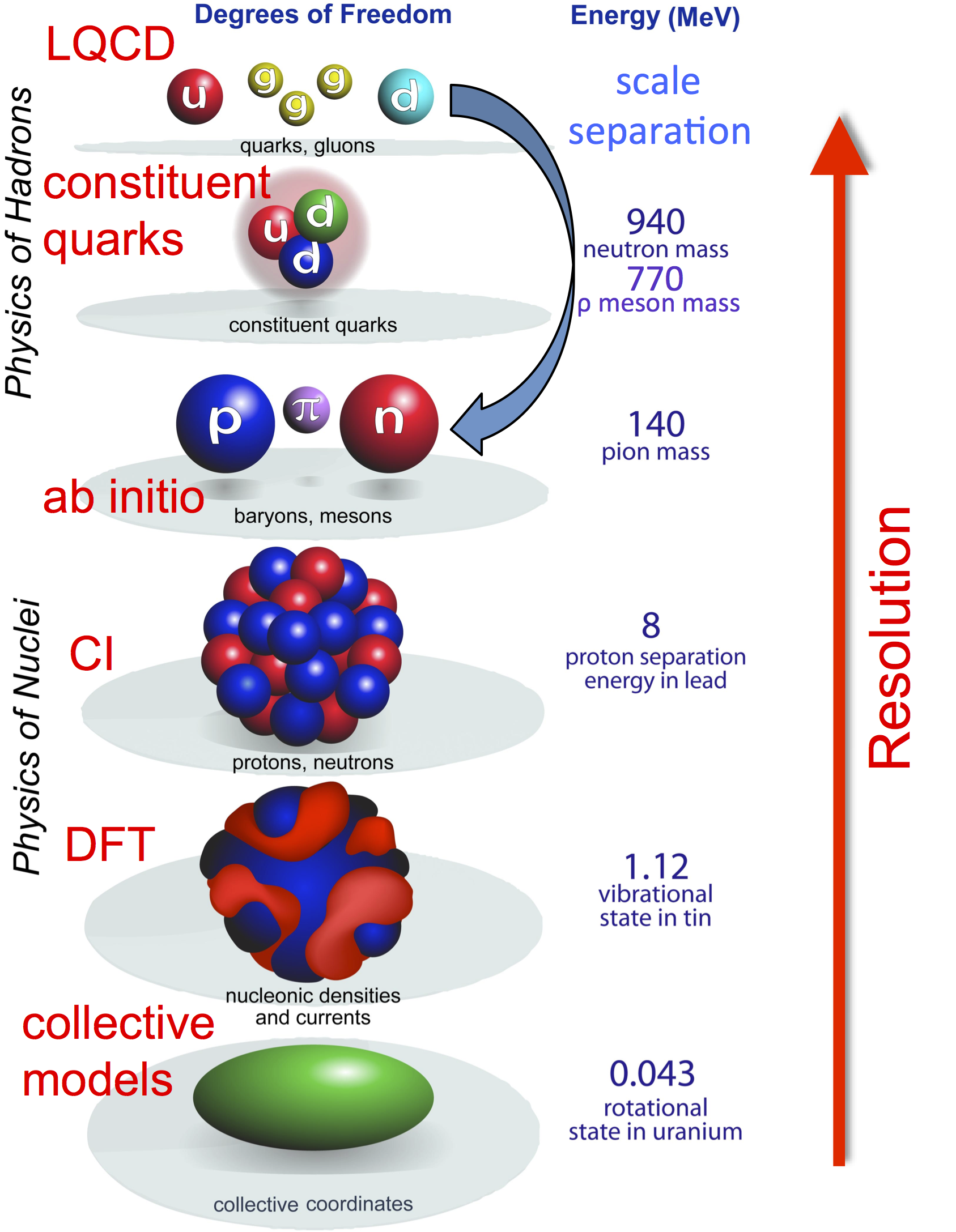
Figure 2.1: Energy scales in nuclear physics. At each step, our resolution changes, and so do the relevant degrees of freedom. This work follows the blue arrow; describing the jump from QCD to ab initio methods which rely on EFTs. Figure from G. F. Bertsch et al [6].

2.3.1 Quantum Chromodynamics (QCD)

Quantum Chromodynamics (QCD) is an SU(3) gauge field theory that describes the strong interactions between quarks and gluons. It was developed throughout the 1970s, as an application of Yang-Mills theory.

The QCD Lagrangian is given by

$$\mathcal{L}=\sum_{q}\bar{\psi}_{q,a}\left(i\gamma^{\mu}\partial_{\mu}\delta_{ab}-g_{s}\gamma^{\mu}t_{ab}^{C}A_{\mu}^{C}-m_{q}\delta_{ab}\right)\psi_{q,b}-\frac{1}{4}F_{\mu\nu}^{A}F^{A\mu\nu}$$ (2.69)

where repeated indices are summed over. The $\gamma^{\mu}$ are the Dirac $\gamma$-matrices. The $\psi_{q,a}$ is the quark field spinors, for quark flavour $q=u,d,s,c,t,\text{or}b$, with corresponding masses $m_{q}$, and a color index $a=1,\cdots,N_{c}=3$, i.e. quarks come with three “color charges.” These quark fields are therefore elements of fundamental representation of SU(3). The $A_{\mu}^{C}$ are the gluon fields, where $\mu$ is once again the Dirac index, and $C=1,\cdots,N_{c}^{2}-1=8$ runs over the 8 kinds of gluons. These gluon fields transform under the adjoint representation of SU(3). The $t_{ab}^{C}$ are the Gell-Mann matrices, defined by the relation

$$\left[t^{A},t^{B}\right]=if_{ABC}t^{C}$$ (2.70)

where $f_{ABC}$ are the structure factors of $SU(3)$. Finally, the field strength tensor $F_{\mu\nu}^{A}$ is defined by

$$F_{\mu\nu}^{A}=\partial_{\mu}A_{\nu}^{A}-\partial_{\nu}A_{\mu}^{A}-g_{s}f_{ABC}A_{\mu}^{B}A_{\nu}^{C}$$ (2.71)

The coupling of the strong interaction is $g_{s}$. These enter into the three fundamental diagrams of QCD: a quark-antiquark-gluon vertex, a three-gluon vertex, and a four-gluon vertex. These diagrams contribute factors of $g_{s}$, $g_{s}$, and $g_{s}^{2}$, respectively.

One peculiarity of QCD is that quarks and gluons cannot be observed as free particles; instead they must be observed as color-neutral (color singlet) states. These can form mesons (a quark-antiquark) and baryons (three quarks). This property is known as “confinement.”

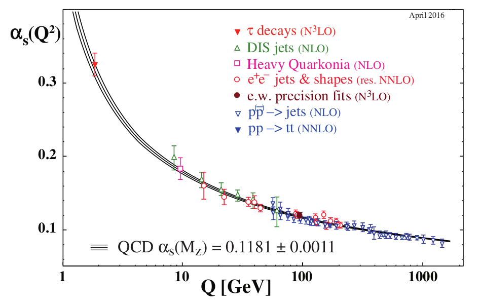
Figure 2.2: The running coupling of QCD. Shown is a plot of the renormalized coupling $\alpha_{s}$ as a function of momentum transfer $Q$. Shown are the numerous experimental and numerical calculations of $\alpha_{s}$, at various $Q$, and the best fit value at the Z-boson mass $M_{Z}$ is presented [26]

Another interesting feature of QCD is that of asymptotic freedom; the strength of the strong interaction gets weaker at higher energies, and stronger at lower energies. This running coupling is shown in Fig. [2.2]. For low energies, QCD is non-perturbative, so it is often the case that computations are done at higher values for the coupling, the extrapolated down to the “physical point”.

2.3.2 Chiral Effective Field Theory

Chiral effective field theory ($\chi$-EFT) and chiral perturbation theory ($\chi$-PT) are built from a low energy effective field theory that was designed to be consistent with the chiral symmetry of the QCD Lagrangian. This chiral symmetry, simply put, is the limit where the quark masses go to zero.

Construction of the chiral Lagrangian starts with considering all terms that are consistent with the approximate chiral symmetry of QCD. This symmetry can be spontaneously broken, giving rise to the Goldstone bosons, the pions.

In this low-energy EFT, the relevant degrees of freedom move from the quarks and gluons to just the hadrons. In $\chi$-EFT, these are taken to be the nucleons. Then, one can work in terms of a power counting scheme in terms of some momentum scale.

If one looks at a given diagram, the behaviour can be analysed by rescaling the external momentum lines $p_{i}\to tp_{i}$ and the quark masses $m_{i}\to t^{2}m_{i}$. Then, Weinberg’s power counting shows that a given digram scales as $t^{D}$ for $D\geq 2$ is the number of vertices in the diagram. For a given $D$, this tells us to what order in the expansion of $\mathcal{L}_{\chi}$ we need.

These expansions tend to work for momentum smaller than the chiral symmetry breaking scale $\Lambda_{\chi SB}\approx 4\pi f_{0}$, where $f_{0}=93$ MeV is the pion decay constant. Additionally, the other scale where $\chi$-PT tends to break down is near the $\rho$ mass, which is $\approx 780$ MeV.

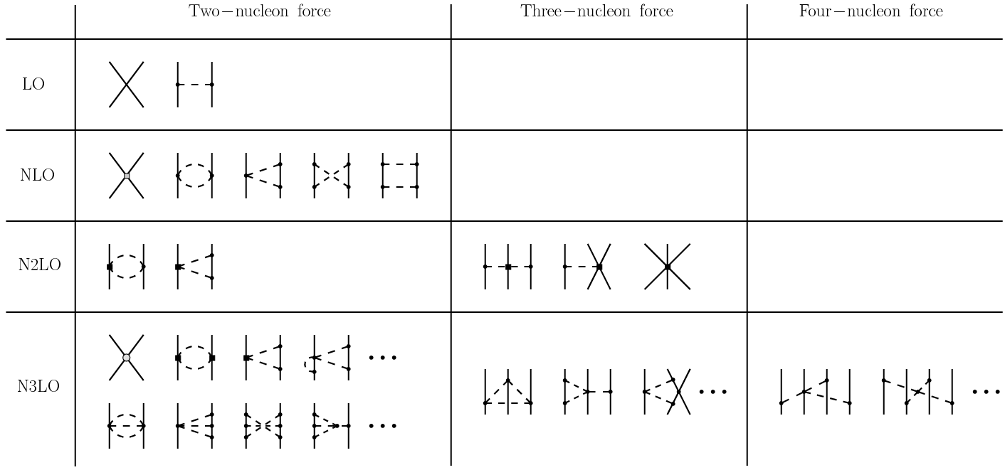
Figure 2.3: An organization of the diagrams in Chiral EFT. Each row indicates the order of the diagram, i.e. how many powers of $(Q/\Lambda)$ the diagram contributes. The solid lines indicate nucleon lines, and the dashed lines indicate pion lines. The columns represent how many nucleons are involved in the process.

Shown in Fig. [2.3] is the organisation of diagrams in terms of this power counting scheme. In the rows are all diagrams which contribute a given power of $(Q/\Lambda)$. In the columns are diagrams which consist of $N$ external nucleon lines.

From this, we can see that the three-nucleon force does not make an appearance until N²LO, which contributes at the $(Q/\Lambda)^{3}$ level.

For more information on chiral perturbation theory or chiral effective field theory, see [65] and [56].

2.3.3 Fitting the LECs to NN Scattering Data

Chiral EFT has several low-energy constants, or LECs, that need to be constrained before any calculations can be done. These are usually done by looking at low-energy scattering experiments between nucleons, such as n-n, n-p, or p-p scattering, or by binding energies of light systems, like the deuteron or alpha particle.

The first step in determining the LECs is to express the relevant operators in terms of angular momentum states. Then, the operators that act on a given partial wave can have their own particular LEC. By looking at the phase shifts, these can be fitted directly with lattice calculations. This section follows the discussion in [48]. For a full discussion, please see this reference.

To start determining the phase shifts on the lattice, we need to re-write the full wavefunction in terms of spherical harmonics. This is done by

$$|r\rangle^{L,L_{z}}=\sum_{\textbf{r}^{\prime}}Y_{L,L_{z}}(\hat{r}^{\prime})\delta(|\textbf{r}^{\prime}|-r)|\textbf{r}^{\prime}\rangle$$ (2.72)

where $r$ is a fixed distance from the origin, and the sum runs over all lattice points. The delta function counts only the lattice points that are a distance $r$ from the origin.

With this definition of the radial wavefunction, the Hamiltonian can be reduce to a form that contains only a single variable, $r$. Then, the phase shifts and mixing angles can be extracted in the region of vanishing potentials. Here, the radial wavefunction can be written in terms of spherical Bessel functions

$$|r\rangle^{L,L_{z}}\approx A_{L}h^{-}_{L}(kr)+B_{L}h^{+}_{L}(kr)$$ (2.73)

where $k=\sqrt{2\mu E}$, $\mu$ is the reduced mass, and $E$ is the energy. The scattering coefficients $A_{L}$ and $B_{L}$ are related to the S-matrix by

$$B_{L}=S_{L}A_{L}$$ (2.74)

with $S_{L}=\exp(2i\delta_{L})$, where $\delta_{L}$ is the phase shift. This phase shift is determined by

$$\delta_{L}=\frac{1}{2i}\log\left(\frac{B_{L}}{A_{L}}\right)$$ (2.75)

Fitting the phase shifts is done using a least-squares minimization. Shown in Fig. [2.4] are the results of fits of the phase shifts and mixing angles for several partial waves, done on a lattice with lattice spacing $a=1.97\text{ fm}$, for the energy range $E_{\text{lab}}\leq 50\text{ MeV}$.

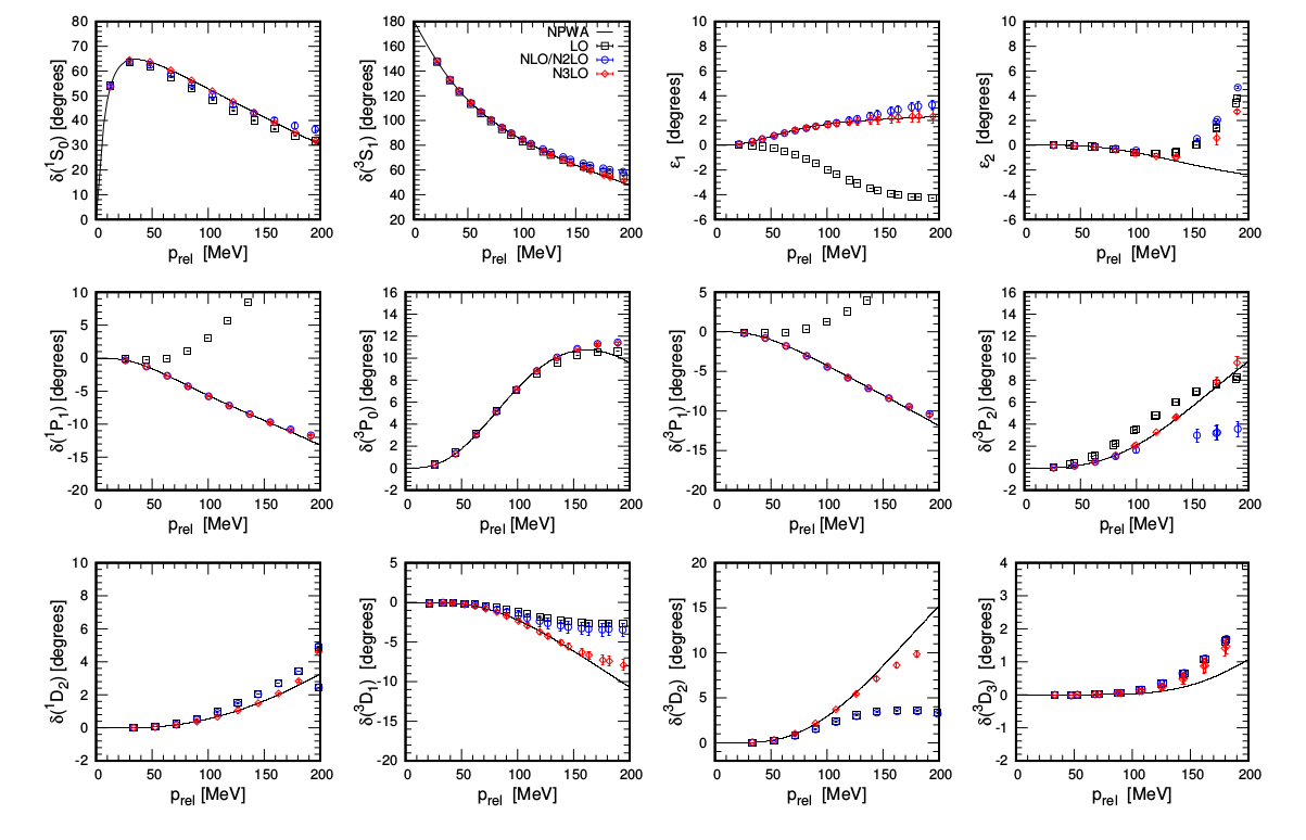
Figure 2.4: Neutron-proton phase shifts and mixing angles, calculated on the lattice, and shown as a function of the relative momenta $p_{\text{rel}}$. Figure courtesy of N. Li [48].

2.4 Monte Carlo Methods

In this section, we will discuss the main methods that we use to evaluate these discretized path integrals.

2.4.1 What is Monte Carlo?

Monte Carlo algorithms are a type of algorithm that involves repeatedly generating random numbers, and using them in some meaningful way. They were named after the city of Monte Carlo in Monaco, since these algorithms have the gambling/rolling dice feel to them.

One of the primary uses of Monte Carlo is in numerically integrating a function. If we consider a function of one variable $f(x)$, over some closed interval $[ab]$, then we can view the integral of this function over this interval

$$\int_{a}^{b}f(x)dx$$ (2.76)

as the area under the curve. All that we need to do is pick points in the domain and range of $f(x)$, and check to see if the point is above or below $f(x)$. Then, the integral can be evaluated as

$$\int_{a}^{b}f(x)dx=\lim_{N\to\infty}\left(\frac{N_{\text{below}}}{N}\right)$$ (2.77)

The other primary use of Monte Carlo algorithm is in sampling probability distributions. For a given continuous probability distribution $\mathcal{P}(x)$ and operator $\mathcal{O}(x)$

$$\left\langle\mathcal{O}\right\rangle=\int\mathcal{P}(x)\mathcal{O}(x)dx=\lim_{N\to\infty}\frac{1}{N}\sum_{i=1}^{N}\mathcal{P}(x_{i})\mathcal{O}(x_{i})$$ (2.78)

That is, any expectation value which involves integrating a quantity over some weight distribution can be expressed as a discrete sum over a finite number of samples pulled from that distribution.

In lattice field theory, this probability distribution is the Boltzmann distribution $e^{-\mathcal{S}}$, and the integration variables are the fermion fields. Now, since there is an infinite sum for each variable being integrated, direct sampling would never work for these lattice field theories. For this, we need more specialized algorithms.

2.4.2 The Sign Problem

Before we hop into the discussion of the Monte Carlo algorithms we use in our simulations, we first make a few remarks about the sign problem.

The sign problem/fermion sign problem/signal-to-noise problem is a common issue that arises in the simulations of fermions, and it is due to the fact that the probability distribution is not necessarily positive-definite. If we consider the expectation values of some operator

$$\langle A\rangle=\frac{\int D\phi A[\phi]p[\phi]}{\int D\phi p[\phi]}$$ (2.79)

with bosonic fields $\phi$, and the probability weight defined by

$$p[\phi]=\det\left(M[\phi]\right)\exp\left(-\mathcal{S}[\phi]\right)$$ (2.80)

which contains the fermion determinant and the Boltzmann weighting factor. When $p[\phi]$ is positive for all $\phi$, this integral is well-defined, and can be evaluated numerically.

However, if $p[\phi]$ is ever non-positive (usually due to a complex $\mathcal{S}$), then the integral becomes highly oscillatory, can cannot reliably be determined numerically. This can be shown if we break the probability weights into a modulus and a phase

$$p[\phi]=\rho[\phi]\exp(i\theta[\phi])$$ (2.81)

and then we move the phase into the definition of the expectation value.

$$\langle A\rangle=\frac{\int D\phi\rho[\phi]\exp(i\theta[\phi])}{\int D\phi\rho[\phi]\exp(i\theta[\phi])}=\frac{\langle A[\phi]\exp(i\theta[\phi])\rangle}{\langle\exp(i\theta[\phi])\rangle}$$ (2.82)

This $\rho[\phi]$ is now strictly real and positive-definite, so can always be interpreted as a probability weight. This phase factor now encodes all of the complex behaviour of the observables and fields. For $\exp(i\theta[\phi])\approx 1$, there is no sign problem, and this expectation value is well-defined. If, however, $\exp(i\theta[\phi])\to 0$, both the numerator and denominator become small, leading to wildly fluctuating estimates for the expectation value.

This problem is an NP-Hard problem, meaning that a general solution to it is likely not possible (see P = NP). Instead, the best we can do is to find ways to circumvent the problem. There are multiple ways to minimize this problem in the context of lattice simulations; meron cluster algorithms [11], the complex Langevin method [1], a density of states method [43], pseudofermions [29], Canonical methods [3, 14], analytic continuation from imaginary chemical potentials [15], fermion bags [9], re-weighting methods [27], sign-optimized manifolds [2], or thimble methods [12, 13]. Each has its own particular formulation, advantages, and disadvantages. In this work, we will show how the eigenvector continuation method can avoid this problem from becoming too much of a problem.

2.4.3 Euclidean Time Projection Monte Carlo

If we are interested in studying the dynamics of a quantum system on the lattice, then it would be natural to look at the time evolution of a system. However, in quantum mechanics, the time evolution operator is simply a phase factor

$$\hat{T}(t_{i}-t_{j})=e^{-i\hat{H}(t_{i}-t_{j})}$$ (2.83)

It is then a “natural” extension to consider the case $t\to i\tau$, which is a Wick rotation for the time variable. This new “time” variable $\tau$ is referred to as the Euclidean time, or projection time. The effect of this transformation is it turns the time projection operator into one that can be calculated easily, as it is a simple exponential decay

$$\hat{T}_{E}(\tau_{i}-\tau_{j})=e^{-\hat{H}(\tau_{i}-\tau_{j})}$$ (2.84)

In Monte Carlo simulations, we keep track of the Euclidean time projection amplitude

$$Z_{N,N}(\tau)\equiv\prod_{\vec{n},n_{t}}\left[\int d_{j}s(\vec{n},n_{t})\right]\langle\Psi^{0,\text{free}}_{N,N}|M_{j}(s,t)\cdots M_{j}(s,0)|\Psi^{0,\text{free}}_{N,N}\rangle$$ (2.85)

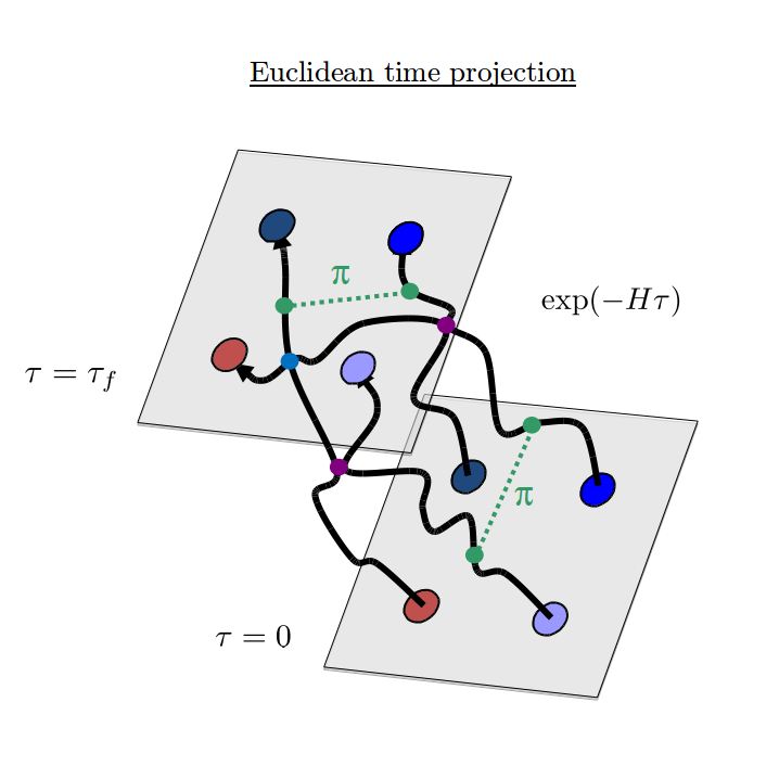
Figure 2.5: Propagation of the many-body state from ($\tau=0$) to a final state ($\tau=\tau_{f}$). During the propagation, particles can interact via any of the chiral forces (LO contact and one-pion exchange shown here.)

Combining this method with the auxiliary fields, we can break the propagation involving many-body interactions (shown in Fig. [2.5]) into the propagation of single particle states through interactions with fluctuating background fields. This is shown in Fig. [2.6].

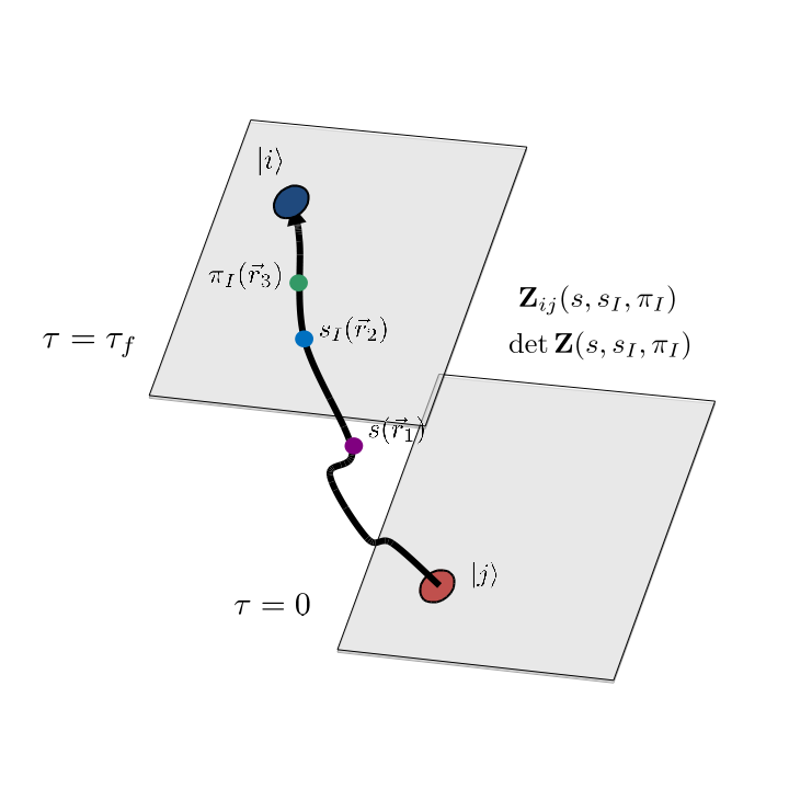
Figure 2.6: Propagation of some initial single-particle state ($\tau=0$) to a final state ($\tau=\tau_{f}$). Along the path, the state interacts with the background auxiliary fields.

We now define an online energy expectation value that depends on the Euclidean time $\tau$

$$E_{N,N}(\tau)=\frac{1}{\alpha_{t}}\log\frac{Z_{N,N}(\tau-a_{t})}{Z_{N,N}(\tau)}$$ (2.86)

Looking at the spectral decomposition of $Z_{N,N}$, we see

$$Z_{N,N}(\tau)=\sum_{k}|c_{N,N}^{k}|^{2}e^{-E_{N,N}^{k}\tau}$$ (2.87)

For the limit of $\tau\to\infty$, the lowest energy eigenstate is the primary contributor to the amplitude, and all the higher energy states are exponentially suppressed.

$$E_{N,N}(\tau)\approx E_{N,N}^{0}+\sum_{k\neq 0}\left(\frac{|c_{N,N}^{k}|^{2}}{|c_{N,N}^{0}|^{2}}\right)\left(\frac{e^{(E_{N,N}^{k}-E_{N,N}^{0})a_{t}}-1}{\alpha_{t}}\right)e^{-(E_{N,N}^{k}-E_{N,N}^{0})\tau}$$ (2.88)

This can be further simplified by noting that the difference between the energy eigenstates $(E_{N,N}^{k}-E_{N,N}^{0})$ is usually smaller than the energy cutoff scale $1/\alpha_{t}$. This can simplify then to

$$E_{N,N}(\tau)\approx E_{N,N}^{0}+\sum_{k\neq 0}\left(\frac{|c_{N,N}^{k}|^{2}}{|c_{N,N}^{0}|^{2}}\right)\left(E_{N,N}^{k}-E_{N,N}^{0}\right)e^{-(E_{N,N}^{k}-E_{N,N}^{0})\tau}$$ (2.89)

With this, we say that the ground state energy $E_{N,N}^{0}$ is the large $\tau$ limit

$$E_{N,N}^{0}=\lim_{\tau\to\infty}E_{N,N}(\tau)$$ (2.90)

2.4.4 Auxiliary Field Monte Carlo

Now that we have shown how to evaluate the ground state energy by propagating single-particle states through Euclidean time, we now wish to show how the auxiliary fields for the transfer matrices are generated.

The auxiliary fields are defined used a Gaussian integral transformation, known as the Hubbard-Stratonovich [35] transformation.

$$\exp\left[-\frac{C\alpha_{t}}{2}(a^{\dagger}(n)a(n))^{2}\right]=\sqrt{\frac{1}{2\pi}}\int_{-\infty}^{\infty}ds\exp\left[-\frac{1}{2}s(n)^{2}+\sqrt{-C\alpha_{t}}s(n)a^{\dagger}(n)a(n)\right]$$ (2.91)

This transformation allows us to decompose two-body interactions into the integral over one-body interactions with a normally-distributed, background field. The only price is the addition of an integral at each lattice site for each interaction to be written in this manner. However, this is where Monte Carlo is well-suited.

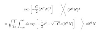
Figure 2.7: A diagram of the Hubbard-Stratonivich transformation. Here, we can express the two-body interaction in terms of a one-body interaction with a fluctuating background field.

For simple contact interactions, the auxiliary field can be directly sampled from a normal distribution

$$P=exp\left(-\frac{1}{2}s(n)^{2}\right)$$ (2.92)

However, for more complicated interactions, like Coulomb or one-pion exchange, we have to work harder. Here, we take as our distribution

$$P=\exp\left(-\mathcal{S}\right)=\exp\left(-\sum_{\vec{n},\vec{n}^{\prime}}s_{1}(\vec{n},n_{t})V^{-1}(\vec{n}-\vec{n}^{\prime})s_{1}(\vec{n}^{\prime},n_{t})\right)$$ (2.93)

where this action is the same as in Eqn. (2.60), except we have removed the constant factor in front as well as the sum over time steps.

This form of the action is difficult to sample by itself, so we factor it into a Gaussian-like form. Defining a $t(\vec{n},n_{t})$ variable, we would like

$$\sum_{\vec{n},\vec{n}^{\prime}}s_{1}(\vec{n},n_{t})V^{-1}(\vec{n}-\vec{n}^{\prime})s_{1}(\vec{n}^{\prime},n_{t})=\frac{\left[t(\vec{n},n_{t})\right]^{2}}{2}$$ (2.94)

so that the probability distribution simplifies to

$$P=\exp\left(-\mathcal{S}\right)=\exp\left(\frac{-\left[t(\vec{n},n_{t})\right]^{2}}{2}\right)$$ (2.95)

By inspection, we see that if we define $t(\vec{n},n_{t})$ as

$$t(\vec{n},n_{t})=\sum_{\vec{n}^{\prime}}V^{-1/2}(\vec{n}-\vec{n}^{\prime})s_{1}(\vec{n}^{\prime},n_{t})$$ (2.96)

we reproduce the original distribution. If we invert this equation to solve for $s_{1}(\vec{n}^{\prime},n_{t})$, we have

$$s_{1}(\vec{n},n_{t})=\sum_{\vec{n}^{\prime}}V^{+1/2}(\vec{n}-\vec{n}^{\prime})t(\vec{n}^{\prime},n_{t})$$ (2.97)

This equation provides a simple prescription for generating a new $s_{1}(\vec{n},n_{t})$. We just need to generate a set of normally-distributed numbers $t(\vec{n},n_{t})$, and plug those in. However, this is a slow process, so using a convolution can speed this updating up tremendously.

If we define $\tilde{u}(\vec{k})$ to be,

$$\tilde{u}(\vec{k},n_{t})=\left(\tilde{V}^{+1/2}(\vec{k})\right)*\left(\tilde{t}(\vec{k},n_{t})\right)$$ (2.98)

where $*$ indicates a convolution, then the auxiliary field $s_{1}(\vec{n},n_{t})$ is simply

$$s_{1}(\vec{n},n_{t})=u(\vec{n},n_{t})$$ (2.99)

where the tilde represents the momentum space representations of each variable. These are obtained through the Fourier transform. With these formulas, the algorithm for updating the field is then:

Step #1: Generate $\tilde{V}^{+1/2}(\vec{k})$. This only needs to be done once, at the beginning of the code.

Step #2: For each $\vec{n},n_{t}$, generate $t(\vec{n},n_{t})$ according to Eqn. (2.96).

$$P\left[t(\vec{n},n_{t})\right]\propto\exp\left\{-\frac{1}{2}\left[t(\vec{n},n_{t})\right]^{2}\right\}$$ (2.100)

Step #3: For each time step $n_{t}$, generate the quantities

$$\tilde{t}(\vec{k},n_{t})=\frac{1}{L^{3/2}}\sum_{\vec{n}}t(\vec{n},n_{t})e^{2\pi i\vec{n}\cdot\vec{k}/L}$$ (2.101)

$$\tilde{u}(\vec{k},n_{t})=\tilde{V}^{+1/2}(\vec{k})\tilde{t}(\vec{k},n_{t})$$ (2.102)

$$s_{1}(\vec{n},n_{t})=\frac{1}{L^{3/2}}\sum_{\vec{k}}\tilde{u}(\vec{k},n_{t})e^{-2\pi i\vec{n}\cdot\vec{k}/L}$$ (2.103)

Once observables are computed using this auxiliary field configuration, go back to step #2 and generate a new configuration. Since the fields are being directly sampled from the respective probability distribution, there is no need for any importance sampling or Metropolis accept/reject stages.

This technique is very straight-forward, but usually not the most optimal way to generate field configurations. For this, we turn to more sophisticated updating algorithms, like Hybrid Monte Carlo.

2.4.5 Hybrid Monte Carlo

Recall, our goal is to calculate the ratio

$$\frac{Z_{N,N}(t-a_{t})}{Z_{N,N}(t)}$$ (2.104)

using a Markov chain Monte Carlo method. For $t=L_{t}a_{t}$, auxiliary field configurations for the base interaction are sampled according to the weight

$$\exp\left\{-U_{j}(s)+2\log\left[|\det\textbf{M}_{j}(s,t)|\right]\right\}$$ (2.105)

where

$$U_{1}(s)=\frac{1}{2}\sum_{\vec{n},n_{t}}\left[s(\vec{n},n_{t})^{2}\right]$$ (2.106)

and

$$U_{4}(s)=0$$ (2.107)

This importance sampling is handled by the Hybrid Monte Carlo (HMC) method [17]. This involves computing molecular dynamics trajectories using the Hamiltonian

$$H_{j}(s,p)=\frac{1}{2}\sum_{\vec{n},n_{t}}\left[p(\vec{n},n_{t})\right]^{2}+V_{j}(s)$$ (2.108)

where $p(\vec{n},n_{t})$ is the conjugate momentum of $s(\vec{n},n_{t})$ and

$$V_{j}(s)=U_{j}(s)-2\log\left[|\det\textbf{M}_{j}(s,t)|\right]$$ (2.109)

The algorithm for updating the field is as follows:

Step #1: Select an arbitrary initial configuration $s^{0}$.

Step #2: Select a configuration $p^{0}$ according to a normal distribution.

$$P\left[p^{0}(\vec{n},n_{t})\right]\propto\exp\left\{-\frac{1}{2}\left[p^{0}(\vec{n},n_{t})\right]^{2}\right\}$$ (2.110)

Step #3: For each $\vec{n},n_{t}$, let

$$\tilde{p}^{0}(\vec{n},n_{t})=p^{0}(\vec{n},n_{t})-\frac{\epsilon_{\text{step}}}{2}\left[\frac{\partial V_{j}(s)}{\partial s(\vec{n},n_{t})}\right]_{s=s^{0}}$$ (2.111)

for some small positive $\epsilon_{\text{step}}$. The derivative of $V_{j}(s)$ is computed using

$$\begin{split}\frac{\partial V_{j}(s)}{\partial s(\vec{n},n_{t})}&=\frac{\partial U_{j}(s)}{\partial s(\vec{n},n_{t})}-\frac{2}{\det\textbf{M}_{j}}\sum_{k,l}\frac{\partial\det\textbf{M}_{j}}{\partial\left[\textbf{M}_{j}\right]_{kl}}\frac{\partial\left[\textbf{M}_{j}\right]_{kl}}{\partial s(\vec{n},n_{t})}\\ &=\frac{\partial U_{j}(s)}{\partial s(\vec{n},n_{t})}-2\sum_{k,l}\left[\textbf{M}_{j}^{-1}\right]_{lk}\frac{\partial\left[\textbf{M}_{j}\right]_{kl}}{\partial s(\vec{n},n_{t})}\end{split}$$ (2.112)

Step #4: For steps $i=0,1,\cdots,N_{\text{step}}-1$, let

$$s^{i+1}(\vec{n},n_{t})=s^{i}(\vec{n},n_{t})+\epsilon_{\text{step}}\tilde{p}^{i}(\vec{n},n_{t})$$ (2.113)

$$\tilde{p}^{i+1}(\vec{n},n_{t})=\tilde{p}^{i}(\vec{n},n_{t})-\epsilon_{\text{step}}\left[\frac{\partial V_{j}(s)}{\partial s(\vec{n},n_{t})}\right]_{s=s^{i+1}}$$ (2.114)

for each $\vec{n},n_{t}$.
Step #5: For each $\vec{n},n_{t}$, let

$$p^{N_{\text{step}}}(\vec{n},n_{t})=\tilde{p}^{N_{\text{step}}}(\vec{n},n_{t})-\frac{\epsilon_{\text{step}}}{2}\left[\frac{\partial V_{j}(s)}{\partial s(\vec{n},n_{t})}\right]_{s=s^{\text{step}}}$$ (2.115)

Step #6: Select a random number $r\in[0,1)$. If,

$$r<\exp\left[-H(s^{N_{\text{step}}},p^{N_{\text{step}}})+H(s^{0},p^{0})\right]$$ (2.116)

then set $s^{0}=s^{N_{\text{step}}}$. Otherwise, leave $s^{0}$ as is.
Once observables are computed using this auxiliary field configuration, go back to step #2 and start a new trajectory. The observable we calculate at each configuration is

$$O_{j}(s,L_{t}a_{t})=\frac{\left[\det\textbf{M}_{j}(s,(L_{t}-1)\alpha_{t})\right]^{2}}{\left[\det\textbf{M}_{j}(s,L_{t}\alpha_{t})\right]^{2}}$$ (2.117)

by taking the ensemble average of this observable over many HMC trajectories, we obtain

$$\frac{Z_{N,N}(t-\alpha_{t})}{Z_{N,N}(t)}$$ (2.118)

2.4.6 Shuttle Algorithm

Now that we have algorithms for generating auxiliary field configurations and propagating the states through Euclidean time, we are ready to put everything together. In older codes, we used to generate all of the auxiliary fields first, then propagate the initial wavefunctions through Euclidean time, and then calculate the expectation values of observables at the middle time-step. This order is not very efficient, and wastes a lot of computational time.

A new algorithm we began to use is the Shuttle algorithm, discussed briefly in [51]. This algorithm instead updates the time steps one at the time, sweeping back and forth from $\tau=0$ to $\tau=L_{t}a_{t}$. The schematic of this method is shown in Fig. (2.8).

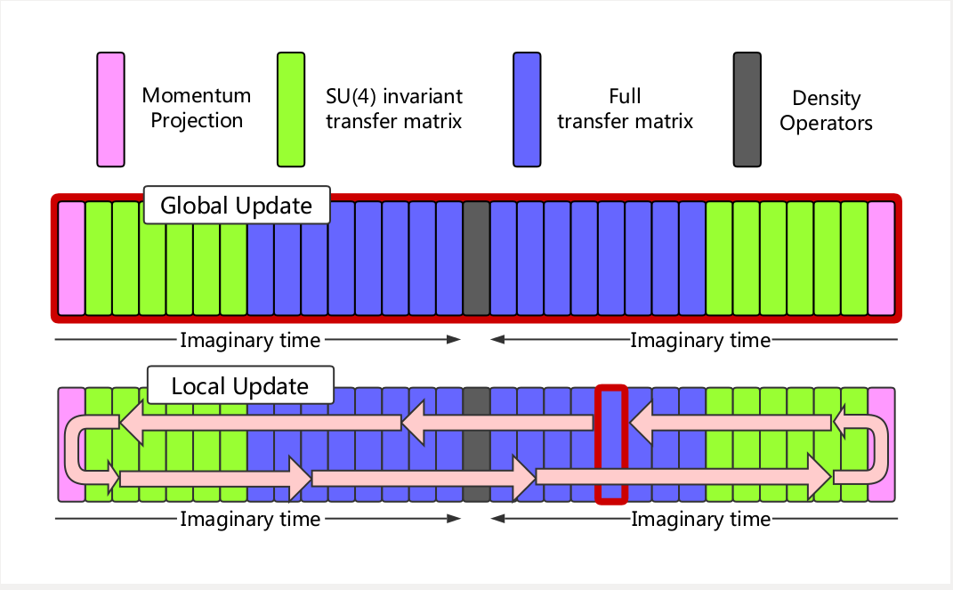
Figure 2.8: Schematic of Shuttle Algorithm. Courtesy of Bingnan Lu (MSU)

The global update here is the older algorithm, and the local update is this new algorithm. On the diagram, the red box shows the ”current” time-step being updated. As this red box moves left and right, new auxiliary fields are generated, using either HMC for the full transfer matrix steps, or the simpler Metropolis updates for the SU(4)-invariant time steps.

When the red box reaches the middle time-step, the expectation value of all of the operators are computed. And finally, when the red box reaches the first or last time step, the initial states are re-updated, and the sweep direction is reversed. Using this algorithm, we can minimize the wasted time during the Monte Carlo simulations.

Chapter 3 Eigenvector Continuation

In this chapter, we discuss the main topic of this dissertation; the Eigenvector Continuation technique. This method begins with some Hermitian Hamiltonian matrix $H$

$$H=H_{0}+cH_{1}$$ (3.1)

with the eigenvectors denoted $|\psi_{j}(c)\rangle$. Generating a power series expansion for $|\psi_{j}(c)\rangle$, we get

$$|\psi_{j}(c)\rangle=\sum_{n=0}^{\infty}|\psi^{(n)}_{j}(0)\rangle c^{n}/n!$$ (3.2)

were $c$ is assumed to be in a region in which this series converges. Suppose that we are interested in a value of $c$ outside of this region. Using just perturbation theory, we would be out of luck. However, suppose that we construct a new series about a point $|w|<|c|$. Then, we could write

$$|\psi_{j}(c)\rangle =\sum_{n=0}^{\infty}|\psi^{(n)}_{j}(w)\rangle\left(c-w\right)^{n}/n!$$ (3.3)

$$|\psi^{(n)}_{j}(w)\rangle =\sum_{m=0}^{\infty}|\psi^{(n+m)}_{j}(0)\rangle w^{m}/m!$$ (3.4)

Combining these, we can obtain

$$|\psi_{j}(c)\rangle=\sum_{n=0}^{\infty}\sum_{m=0}^{\infty}\left(c-w\right)^{n}w^{m}|\psi^{(n+m)}_{j}(0)\rangle/m!n!$$ (3.5)

This multi-series expansion is the heart of the eigenvector continuation method. In a sense, we now have an expression for $|\psi_{j}(c)\rangle$ with a wider area of convergence. Now, from a numerical standpoint, the analogue of derivatives of the eigenvectors at $c=0$ are the finite differences, i.e. computing the eigenvectors at multiple small values for the couplings. In this work, we will refer to these eigenvectors as EC eigenvectors or training eigenvectors.

Once we obtain these eigenvectors, we can form them into a projection operator $P$ and project the Hamiltonian $H$ at some target coupling $C_{\odot}$ into this lower-dimensional subspace. We call the projected Hamiltonian $M=P^{\dagger}HP$, and the norm matrix $N=P^{\dagger}P$. Then, we solve the generalized eigenvalue problem

$$M\vec{v}=\lambda_{i}N\vec{v}$$ (3.6)

The lowest eigenvalue of this system is called the EC estimate for the ground state energy, and the ground state eigenvector in the full space can be reconstructed from the projection operator

$$|\psi_{0}(C_{\odot})\rangle=P\vec{v}_{0}$$ (3.7)

From here, we briefly discuss how these techniques are implemented numerically, with a side discussion about the computational costs. The computation associated with the eigenvector continuation method hinges on the computation of the training eigenvectors for a few values of the coupling $c$. If these can be accurately obtained, and if the overlaps between any two EC training eigenvectors are not nearly 1, then the method will be applicable.

3.1 Mathematical Formalism

We start this discussion by considering a finite-dimensional linear space and a single parameter family of Hamiltonian matrices

$$H(c)=H_{0}+cH_{1}$$ (3.8)

where $H_{0}$ and $H_{1}$ are Hermitian. Let $|\psi_{j}(c)\rangle$ denote the eigenvectors of $H(c)$ with corresponding eigenvalues $E_{j}(c)$. Since $H(c)$ is Hermitian for real $c$, each $E_{j}(c)$ is strictly real, and thus there are no singularities on the real axis.

Now, we can expand $E_{j}(c)$ and $|\psi_{j}(c)\rangle$ as power series about $c=0$.

$$E_{j}(c) =\sum_{n=0}^{\infty}E_{j}^{(n)}(0)c^{n}/n!$$ (3.9)

$$|\psi_{j}(c)\rangle =\sum_{n=0}^{\infty}|\psi^{(n)}_{j}(0)\rangle c^{n}/n!$$ (3.10)

where the superscript $(n)$ refers to the n-th derivative. This is the approach of perturbation theory. These series are said to converge for all $|c|<|z|$, where $z$ and its complex conjugate are the nearest singularities to $c=0$ in the complex plane.

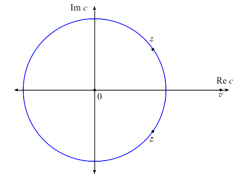
Figure 3.1: Diagram of convergence region for Eqn. (3.2)

If we are interested in points $|c|\geq|z|$, perturbation theory is no longer applicable. We can instead construct an analytic extension of Eqn. (3.2) by constructing a new series about the point $c=w$, where $w$ is real and $|w|<|z|$.

$$|\psi_{j}(c)\rangle =\sum_{n=0}^{\infty}|\psi^{(n)}_{j}(w)\rangle\left(c-w\right)^{n}/n!$$ (3.11)

$$|\psi^{(n)}_{j}(w)\rangle =\sum_{m=0}^{\infty}|\psi^{(n+m)}_{j}(0)\rangle w^{m}/m!$$ (3.12)

Combining these, we can obtain

$$|\psi_{j}(c)\rangle=\sum_{n=0}^{\infty}\sum_{m=0}^{\infty}\left(c-w\right)^{n}w^{m}|\psi^{(n+m)}_{j}(0)\rangle/m!n!$$ (3.13)

that is, the eigenvector $|\psi_{j}(c)\rangle$, can be expressed as a linear combination of the eigenvectors $|\psi_{j}(0)\rangle$ in the region $|c|<|z|$ and the circular region $|c-w|<|z-w|$ centered at $w$.

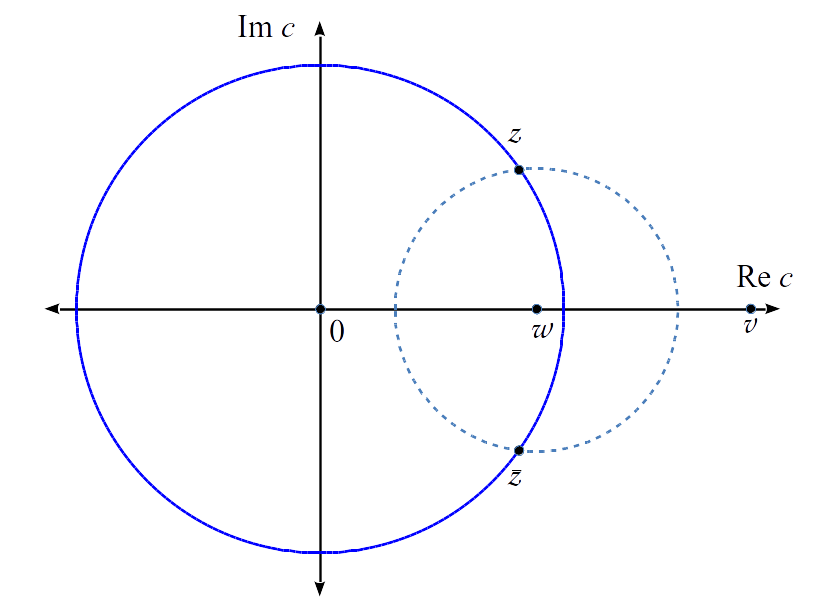
Figure 3.2: Diagram of Extended Convergence Region, Eqn. (3.5)

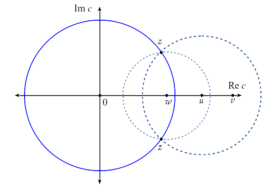
Figure 3.3: Extending the Convergence region to include the point $c=v$

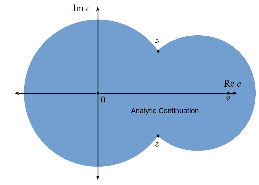
Figure 3.4: Final region of convergence

Analytic function theory help us understand why this technique works. Although in the original expansion for $|\psi_{j}(c)\rangle$ failed to converge for $|c|<|z|$, using the analytic extension Eqn. (3.5) allowed us to express a new series in terms of the original series, to arbitrary accuracy. This process can be repeated, until the target value of the coupling $c=v$ is within the analytically-extended convergence region. The number of vectors required is determined by the number of expansions needed in the analytic continuation, and the order-by-order convergence of each series expansion.

In cases where there are singularities near the real axis, the convergence of these series can be accelerated by including multiple eigenvectors at each value of the coupling. Let us focus on a single eigenvector and eigenvalue of $H(c)$, which we label as $|\psi_{1}(c)\rangle$ and $E_{1}$, respectively. Furthermore, let D be the Riemann surface associated with $|\psi_{1}(c)\rangle$. We will assume that $|\psi_{1}(c)\rangle$ is analytic everywhere except for branch point singularities at $c=z$ and $c=\bar{z}$.

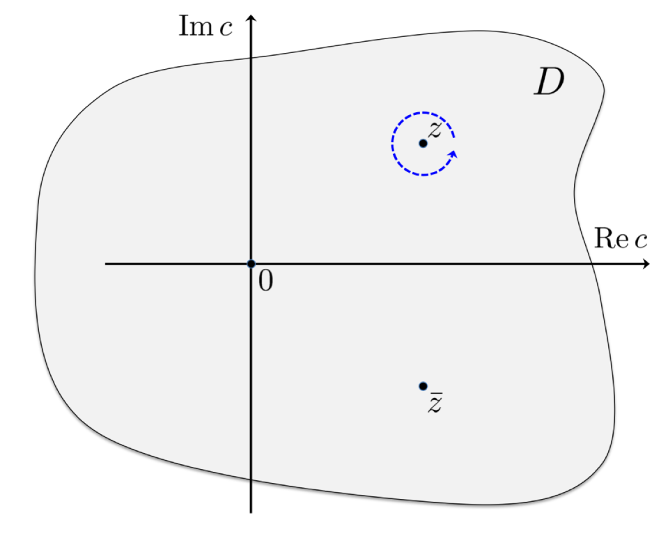
Figure 3.5: D is a finite region of the Riemann surface associated with the vector $|\psi_{1}(c)\rangle$. We assume $|\psi_{1}(c)\rangle$ is analytic everywhere except for branch point singularities at $z$ and $\bar{z}$. The dashed blue line shows the path traced around $z$.

Since the matrix elements of $H(c)$ are analytic everywhere, the characteristic polynomial of $H(c)$ is also analytic everywhere. We now consider what happens when traversing a closed loop around one of these branch points, as in Fig. [3.5]. The effect this process has on the eigenvectors and eigenvalues we will call the monodromy transformation $T(z)$.

We consider the case in which the $E_{1}(z)$ is a unique eigenvalue of $H(z)$. In this case, $T(z)$ transforms the eigenvector $|\psi_{1}(c)\rangle$ to a vector which is proportional to $|\psi_{1}(c)\rangle$. To remove the proportionality constant, we pick some state $|f>$ in the linear space such that $\langle f|\psi_{1}(c)\rangle\neq 0$ for all points $c\in D$. This renormalized eigenvector can then be defined as

$$|\phi_{1}(c)\rangle=\frac{1}{\langle f|\psi_{1}(c)\rangle}|\psi_{1}(c)\rangle$$ (3.14)

Since $\langle f|\phi_{1}(c)\rangle=1$ for all $c\in D$, the transformation $T(z)$ transforms $\langle f|\phi_{1}(c)\rangle$ into itself. Therefore, $|\phi_{1}(c)\rangle$ is also an invariant of the transformation. While $|\psi_{1}(c)\rangle$ has a branch point singularity at $c=z$, the renormalized eigenvector now is analytic at $c=z$. Since the linear space spanned by $|\phi_{1}(c)\rangle$ is identical to the linear space spanned by $|\psi_{1}(c)\rangle$, it is clear that the singularities in the eigenvector normalization have no effect on the eigenvector continuation method.

We now consider the case in which $E_{1}(z)$ is not a unique eigenvalue of $H(z)$. In this case, the transformation $T(z)$ can result in a permutation of eigenvalues that are degenerate at $c=z$. Without loss of generality, we will assume that $T(z)$ induces a permutation cycle involving $k$ eigenvalues that we label $E_{1}(c),E_{2}(c),\cdots,E_{k}(c)$. With this notation, the monodromy transformation produces the cyclic permutation

$$T(z):E_{1}(z)\to E_{2}(z)\to\cdots\to E_{k}(z)\to E_{1}(z)$$ (3.15)

The case $k=1$ will lead to the same conclusion as the unique eigenvalue case. We will focus on the case $k>1$. Let us label the image of $|\phi_{1}(c)\rangle$ under this transformation as $|\phi_{2}(c)\rangle$, an eigenvector of $H(z)$ with eigenvalue $E_{2}(z)$. We continue the labelling in this manner such that the transformation on the eigenvectors has the form

$$T(z):\phi_{1}(c)\rangle\to\phi_{2}(c)\rangle\to\cdots\to\phi_{k}(c)\rangle\to\phi_{1}(c)\rangle$$ (3.16)

The last entry in the cycle is $\phi_{1}(c)\rangle$ due to the fact that $\langle f|\phi_{1}(c)\rangle$ is single-valued under the transformation $\left[T(z)\right]^{k}$.

We note that the linear combinations

$$|\gamma_{n}(c,z)\rangle=\sum_{j=0}^{k-1}e^{i2\pi nj/k}|\phi_{j}(k)\rangle$$ (3.17)

for $n=0,\cdots,k-1$ are the eigenvectors of the monodromy transformation with eigenvalues $e^{-i2\pi n/k}$. We can now renormalize each of these eigenvectors so that the branch point singularity at $c=z$ is removed for each n

$$|\gamma^{\prime}_{n}(c,z)\rangle=e^{n\log(c-z)/k}|\gamma_{n}(c,z)\rangle$$ (3.18)

These $|\gamma^{\prime}_{n}(c,z)\rangle$ vectors are now analytic at $c=z$. In essence, what we have done is made linear combinations of the eigenvectors in which all of the non-integer fractional powers of $c-z$ have been removed. In a similar fashion, we can construct the vectors $|\gamma^{\prime}_{n}(c,\bar{z})\rangle$ that are analytic at $c=\bar{z}$.

Let us now return to the discussion of performing eigenvector continuation with an EC subspace consisting of the k eigenvectors, $|\psi_{1}(c_{i})\rangle,|\psi_{2}(c_{i})\rangle,\cdots,|\psi_{k}(c_{i})\rangle$ for each sampling point $c_{i}$. We note that the singularities at $c=z$ and $c=\bar{z}$ do not cause convergence problems when when determining $|\psi_{1}(c)\rangle$. This is because $|\psi_{1}(c)\rangle$ can be written as a linear combination of vectors $|\gamma^{\prime}_{n}(c,z)\rangle$ that are analytic at $c=z$. Thus, to accelerate convergence near a branch point singularity, the EC subspace should contain all the eigenvectors whose Riemann sheets become intertwined at the branch point.

3.2 Algorithms

The strategy of eigenvector continuation is to construct a set of wavefunctions for different values of the couplings (called the training data or training vectors,) which are used to form a “low-dimensional” subspace that constrains the trajectory of $|\psi_{j}(c)\rangle$. We start with the smallest eigenvalue $E_{1}$ and corresponding eigenvector $|\psi_{1}(c)\rangle$ of the Hamiltonian $H(c)$. The approach will be to sample several values of the coupling $c=c_{i}$, $i=1,\cdots,\mu$, where we use $\mu$ to denote the “order” of the EC method.

The reason for this is that in the limit of small steps between the $c_{i}$’s, the derivatives in the multi-series EC expansion can be approximated by finite differences, and the space spanned by the eigenvectors at various couplings will be approximately identical to the derivatives of the eigenvectors at zero coupling.

This approach gives us $\mu$ eigenvectors $|\psi_{1}(c_{i})\rangle$ with which to form the EC subspace. The couplings $c_{i}$ are chosen to be such that $|\psi_{1}(c_{i})\rangle$ can be accurately computed. If it is the case that $|\psi_{1}(c_{i})\rangle$ cannot be accurately computed for any $c_{i}$, then eigenvector continuation will not be possible.

We assume that $c=c_{\odot}$ is the target value of the coupling, where we wish to determine $E_{1}(c_{\odot})$ and $|\psi_{1}(c_{\odot})\rangle$, and that direct computation of these quantities is not feasible.

The core algorithm of eigenvector continuation starts by forming a $\mu\times\mu$ norm matrix N by taking the inner products between each of the EC wavefunctions

$$N_{i,i^{\prime}}=\left\langle\psi_{1}(c_{i^{\prime}})|\psi_{1}(c_{i})\right\rangle$$ (3.19)

and the matrix elements of $H(c_{\odot})$

$$M_{i,i^{\prime}}=\left\langle\psi_{1}(c_{i^{\prime}})|H(c_{\odot})|\psi_{1}(c_{i})\right\rangle$$ (3.20)

Then, we can solve the generalized eigenvalue problem, which consists of solving the equation

$$\hat{M}\vec{v}=\lambda\hat{N}\vec{v}$$ (3.21)

The smallest eigenvalue $\lambda_{0}$ is the EC estimate for $E_{1}(c_{\odot})$, and the estimate for $|\psi_{1}(c_{\odot})\rangle$ can be constructed by the equation

$$|\psi_{1}(c_{\odot})\rangle=P\vec{v}_{1}$$ (3.22)

where $P$ is the projection operator, an $N\times\mu$ matrix whose columns are the training eigenvectors.

In the Monte Carlo simulations, it is sometimes advantageous to split $M$ into two pieces; one containing the base interactions $M_{0}$, and the other containing the term that has the coupling being varied $M_{\text{EC}}$. Then, we can compute the EC estimate for the energy for arbitrary target coupling $C_{\odot}$ by computing the generalized eigenvalues of

$$(M_{0}+C_{\odot}M_{\text{EC}})\cdot\vec{v}=u\cdot N\cdot\vec{v}$$ (3.23)

This can be done as a post-processing step, saving time during the simulation itself.

One issue that we run into while implementing the eigenvector continuation algorithm is in the inversion of the norm matrix required for the generalized eigenvalue problem. The norm matrix is constructed by taking the overlaps between each of the EC eigenvectors, a la Eqn. (3.19). If these overlaps are too close to unity, i.e. if the EC eigenvectors are too similar, then this norm matrix will become singular, and thus non-invertible. This provides a strict numerical bound to this technique.

To illustrate this problem, we take as an example the Lipkin model (discussed in Section 4.4). We perform a computation to 3rd order EC, computing 3 training eigenvectors with which we form our norm matrix. These three eigenvectors are taken to have couplings that are integer multiples of some step size, i.e. $C_{i}=0\Delta C,1\Delta C,...,i\Delta C$. As we vary $\Delta C$, we expect the overlaps between these wavefunctions to become smaller, and the norm matrix to become less singular. In Fig [3.6], we show the 2nd eigenvalue of this norm matrix.

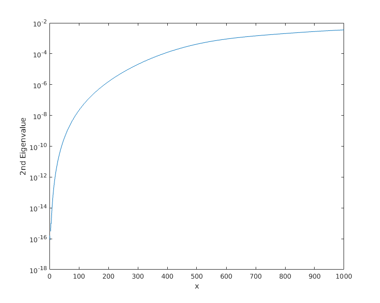
Figure 3.6: 2nd Eigenvalue of EC norm matrix, as a function of the step size between values of the couplings used to generate the EC eigenvectors. Here, the coupling step size is $\Delta C=0.001x$.

This second eigenvalue is a diagnostic about the invertibility of the norm matrix. It will tend towards zero if the matrix becomes singular, and will become larger as the overlaps between the EC eigenvectors become smaller. It is difficult to tell how small of an eigenvalue is “too small”; in our experience, it depends on the system.

To demonstrate the effect this problem has on the extracted ground state wavefunctions and energies, we show a plot of the EC ground state energy estimate at a target coupling of $NV/\epsilon=1.0$, s well as the overlaps of the exact ground state wavefunction with the EC estimate for the wavefunction. In Fig. [3.7], we show the overlaps of the two wavefunctions. In order to plot it in a readable way, we choose to plot one minus the overlap, $1-<\psi_{0}|\psi_{EC}>$ on a log scale, so the estimate can be shown to get exponentially better as the norm matrix becomes less singular.

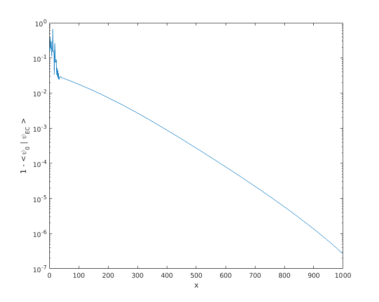
Figure 3.7: Overlap of EC wavefunction with exact ground state.

In Fig. [3.8], we show the estimates for the ground state energy of this system. If the norm matrix is singular or ill-conditioned, this estimate will be impossible or very noisy. Here, we see that the small $\Delta C$ estimates are very chaotic, and it takes a while to converge to a steady value.

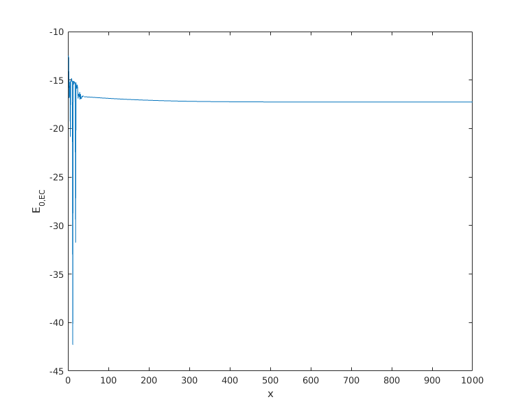
Figure 3.8: EC estimate for ground state energy vs EC coupling step size

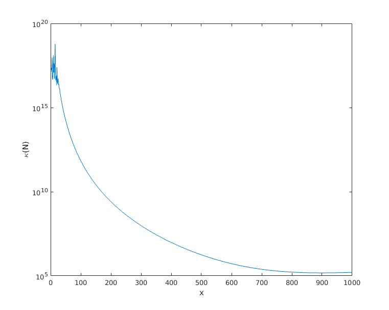
Figure 3.9: Here, we show the condition number of the norm matrix for 3rd order EC, in the Lipkin model. A condition number $\approx 1$ means the matrix can be inverted with no loss of precision, whereas a large condition number indicates numerical instability during the inversion procedure.

Another diagnostic that is useful in determining the stability of the algorithm is the condition number of the norm matrix. This condition number is defined as the ratio of the norms of the largest eigenvalue to the smallest eigenvalue

$$\kappa(N)=\frac{||\max{\lambda_{i}}||}{||\min{\lambda_{i}}||}$$ (3.24)

which is denoted $\kappa$. This condition number usually indicates the loss of precision that any algorithm relying on inverting the matrix would have. $\kappa\approx 1$ would be able to be inverted with no loss of precision, whereas $\kappa\to\infty$ would lose all information. This definition is rather loose, but still can be helpful. In Fig. [3.9], we show the condition number of the same Lipkin model system, at 3rd order EC, plotted as a function of the EC coupling step size $\Delta C$.

Welford’s online algorithm [70] was used to extract more stable estimates for the average and error, compared to the standard Jackknife analysis. This algorithm is an online, iterative method in which running values for the mean $\bar{x}$ and variance $\sigma^{2}$ are kept track of, and updated for new samples $x$ are obtained

$$\bar{x}_{n} =\bar{x}_{n-1}+\frac{x_{n}-\bar{x}_{n-1}}{n}$$

$$M_{2,n} =M_{2,n-1}+(x_{n}+\bar{x}_{n-1})(x_{n}-\bar{x}_{n})$$ (3.25)

$$\sigma^{2}_{n} =\frac{M_{2,n}}{n-1}$$

This algorithm is well-suited to run alongside Monte Carlo simulations, since averages and errors can be updated on the fly, rather than completely re-evaluated after each sample.

We now demonstrate how this algorithm is implemented in our Monte Carlo simulations. This is shown diagrammatically in Figs. [3.10] and [3.11]. First, we start by running the code in parallel, using MPI, such that we have $N$ processors (or cores) each running a copy of the code with different initial random seeds. As we generate Monte Carlo configurations, we group together a large number of configurations, and compute an average on each core (Step #1). Assuming each Monte Carlo configuration is sampled from the same probability distribution, these averages is guaranteed by the central limit theorem to be normally distributed. We would then be able to compute a global average and variance/standard deviation from the data across all cores.

In the eigenvector continuation method, we need to do some computation before we average over the different cores, however. Here, we perform the needed eigenvalue solving, and extract the EC estimates for the ground states. Now, we have an estimate for the energy on each core. To begin applying the online algorithm, we will first average all of the EC estimates on each core into a single value (Step #3). Then, Eqn. (3.25) tell us how to update the global moving average and population variance (Step #4). After this step, we go back to Step #1, and repeat until the average is converged and the errors are low.

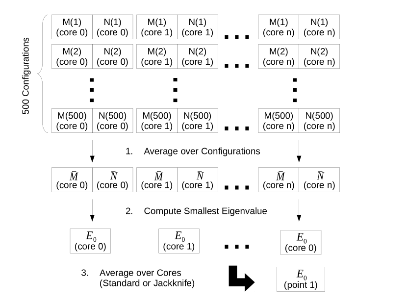
Figure 3.10: Steps #1 - #3 for the implementation of the online algorithm

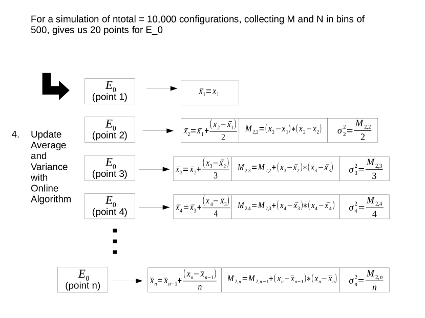
Figure 3.11: Step #4 for the implementation of the online algorithm

In Fig. [3.12], we show a comparison of this method with the conventional jackknife analysis. We plot the estimates of the Coulomb energy shift in ⁴He, computed perturbatively (COUL) and via direct calculation (EC), as a function of the number of Monte Carlo steps. On the top graph, both estimates are computed via a jackknife analysis over the different CPUs. On the bottom graph, the same perturbative result is plotted, but the EC estimate is averaged via the online algorithm.

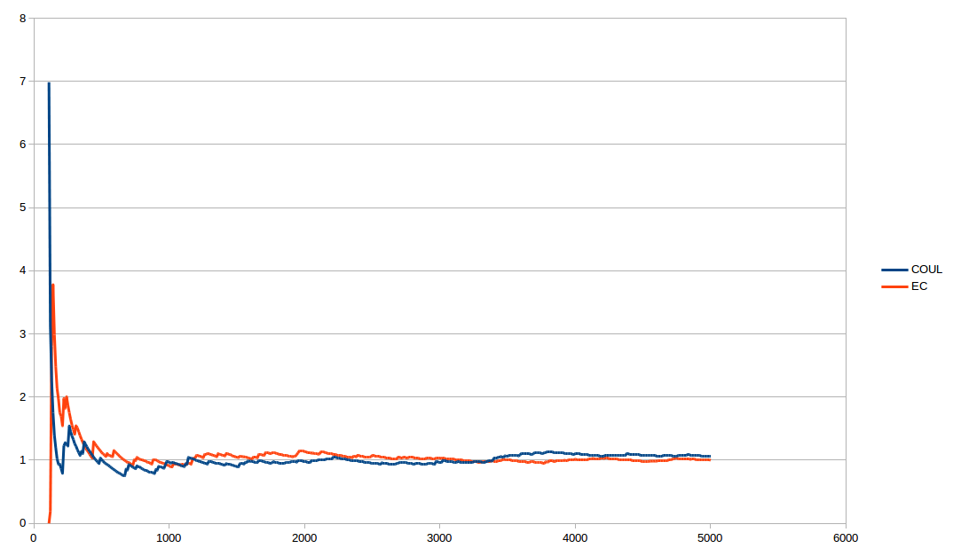
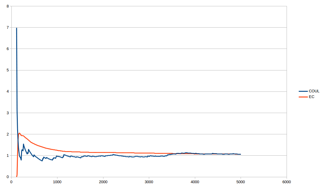
Figure 3.12: Plots of the perturbative Coulomb energy shift in ⁴He computed with a jackknife analysis (in blue), versus the eigenvector continuation estimate for the Coulomb energy shift (orange). On the top plot, the EC estimate was done with a jackknife analysis, and on the bottom, it was done using the online algorithm.

3.3 Implementation and Computational Cost

For the most part, Monte Carlo results detailed in this work were done using a modified version of the MCLEFT code [51], developed by B. Lu (MSU). The modifications were done in Fortran 95, and consisted of a module file containing all the necessary subroutines.

In these codes, the bulk of the work is in generating the auxiliary field configurations, and propagating the initial single-particle wavefunctions through Euclidean time via transfer matrices. These single particle wavefunctions have a spin index, isospin index, and in the modified code, an EC order index. From this we, expect the computational cost of the eigenvector continuation code to be directly proportional to the EC order.

At the middle timestep, we insert various operators to perturbatively calculate various quantities, like energies from higher order Chiral forces, isospin symmetry breaking terms, Galilean invariance restoration terms, etc. These involve forming Slater determinants out of the propagated single-particle states. Due to the size of these determinants, we only store their logarithm. To extract the EC estimates for the energy, we use the BLAS routine DSYGV. Since our projected matrix is a Hamiltonian matrix, we only keep the real part, since the imaginary parts should trend to zero.

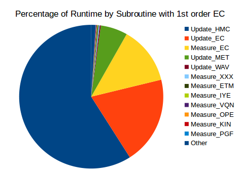
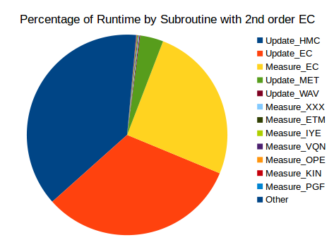
Figure 3.13: gprof breakdown of the computational time spent in major subroutines in the MCLEFT code. At 1st order, the overall time spent in the EC subroutines is about 32%, and at 2nd order, that increases to 56%

In Fig. [3.13], we show the results of profiling this code with gprof for a fixed number of MC steps. UPDATE routines involve generation of the auxiliary fields and propagation of the wavefunctions through time. MEASURE routines involve the computation of observables using the wavefunctions at the center time-step. Subroutines with the suffix EC are routines used in the eigenvector continuation method. From here, we see a rapid growth in the overall time used by the EC method by the time that we have reached 2nd order.

Routine	1st Order EC	2nd Order EC	3rd Order EC
Update_HMC	67.79	66.37	67.52
Update_EC	22.74	58.29	69.96
Measure_EC	14.93	46.09	132.53
Update_MET	6.96	6.76	6.85
Update_WAV	0.31	0.27	0.33
Measure_XXX	0.26	0.25	0.25
Measure_ETM	0.22	0.21	0.21
Measure_IYE	0.18	0.17	0.17
Measure_VQN	0.15	0.13	0.18
Measure_OPE	0.03	0.02	0.03
Measure_KIN	0.12	0.12	0.12
Measure_PGF	0.06	0.02	0.02
Other	1.12	2.62	4.90
Total	114.63	180.08	280.08

Table 3.1: Tabulated results from gprof

This rapid scaling is in part due to the exponential growth in the number of combinations you can form the eigenvectors into subspaces with. If we compute $N$ eigenvectors, and form a subspace out of $m$ of them, there are

$$\text{\# of Choices}=\binom{N}{m}=\frac{N!}{m!(N-m)!}$$ (3.26)

number of choices, which escalates for large $N$. However, if we only pick a particular set of the $N$ eigenvectors to form the subspace out of, the computation time spent can be reduced.

We now show how the EC algorithm scales as a function of the lattice volume. We run the code for fixed number of Monte Carlo steps (100 in this case), a fixed number of particles ($N_{f}$ = 4), and a fixed size of the lattice in the temporal direction ($L_{t,in}=20$,$L_{t,out}=20$). Here, we expect the primary term to be proportional to the lattice volume $L^{3}$. We take our fitting function to be a cubic:

$$T(L)=aL^{3}+bL^{2}+cL$$ (3.27)

with the y-intercept set to zero. This fit is done using a least-squares regression.

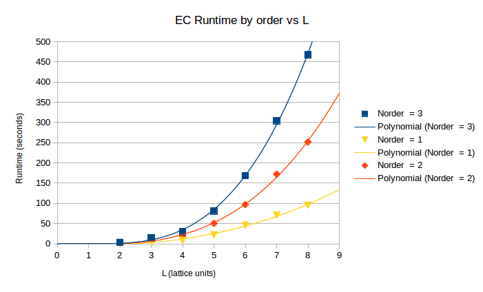
Figure 3.14: Plot of the computational cost/time used by the EC method, as a function of the length of the edges the lattice L. This was done for a fixed number of particles (N=4), and a fixed number of timesteps (Ltinner = 20, Ltouter = 20).

EC Order	$a$ (cubic term)	$b$ (quadratic term)	$c$ (linear term)	$R^{2}$
1st	0.0729667392	1.4274807737	-3.8672850799	0.9972665119
2nd	0.6035009969	-0.7136869805	-1.0474019912	0.9990421919
3rd	1.4201400218	-4.4940652917	4.021016857	0.9995114091

Table 3.2: Coefficients of best polynomial fits to computational cost of the EC algorithm, as a function of the size of the lattice L. Since there are $L^{3}$ points, we expect the leading term to be proportional to $L^{3}$. We don’t expect other terms, but present them for completeness.

We now look at the scaling of the algorithm with respect to the number of particles $N_{f}$. Like before, we fix the number of Monte Carlo steps (100), the spatial size of the lattice ($L=4$), and the size of the lattice in the temporal direction ($L_{t,in}=20$,$L_{t,out}=20$). This time, we expect a small term proportional to $N_{f}^{2}$, and a larger term proportional to $N_{f}$. We then take our fitting function to be a quadratic:

$$T(N_{f})=aN_{f}^{2}+bN_{f}$$ (3.28)

with the intercept set to zero as well.

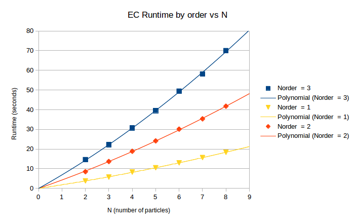
Figure 3.15: Plot of the computational cost/time used by the EC method, as a function of the number of particles in the system. This was done for fixed lattice volume (L=4), and a fixed number of timesteps (Ltinner = 20, Ltouter = 20).

EC Order	$a$ (quadratic term)	$b$ (linear term)	$R^{2}$
1st	0.0649337121	1.7797578463	0.9999319128
2nd	0.1325730519	4.1616152597	0.9999292763
3rd	0.255174513	6.6464975649	0.9999057979

Table 3.3: Coefficients of best polynomial fits to computational cost of the EC algorithm, as a function of the number of particles in the system $N_{f}$. We expect a small term proportional to $L^{2}$, from the matrix elements, and a large linear term, since we keep track of single-particle wavefunctions.

Chapter 4 Applications to Nuclear Systems

In this chapter, we discuss all the applications of eigenvector continuation to nuclear systems that have been investigated so far. We start with the initial investigations into the Bose-Hubbard model and infinite neutron matter. Then, we discuss the main project of computing the contribution of the Coulomb interaction to the ground state energy in light nuclei. Then, we look at a much older model of nuclear structure; the Lipkin-Meshkov-Glick Hamiltonian.

4.1 Bose-Hubbard Model

The Bose-Hubbard model in three dimensions [30] consists of a system of identical bosons on a three-dimensional cubic lattice. The Hamiltonian has a hopping term, controlling the nearest-neighbour hopping of each boson, a potential term proportional to U controlling the pairwise interaction between bosons on the same site, and a chemical potential $\mu$, and it has the form

$$H=-t\sum_{\langle\textbf{n},\textbf{n'}\rangle}a^{\dagger}(\textbf{n'})a(\textbf{n})+\frac{U}{2}\sum_{\textbf{n}}\rho(\textbf{n})\left[\rho(\textbf{n})-\textbf{1}\right]-\mu\sum_{\textbf{n}}\rho(\textbf{n})$$ (4.1)

where $a^{\dagger}(\textbf{n})$ and $a(\textbf{n})$ are the creation and annihilation operators for bosons at the lattice site n, the first summation is over nearest-neighbour pairs $\langle\textbf{n},\textbf{n'}\rangle$, and $\rho(\textbf{n})=a^{\dagger}(\textbf{n})a(\textbf{n})$ is the density operator.

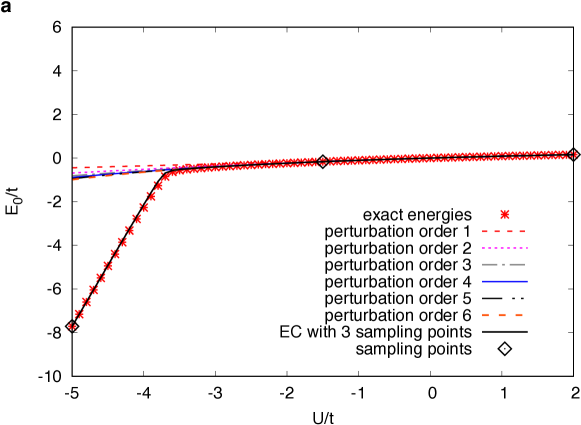
Figure 4.1: Ground state energy for the Bose-Hubbard model, computed by exact diagonalization and by perturbation theory.

We consider a system of four particles on a $4\times 4\times 4$ lattice. To illustrate why we chose this problem, we first try using perturbation theory to find the ground state energy eigenvalue $E_{0}$ in units of the hopping parameter $t$. In Fig. [4.1], we show the ground state energy $E_{0}/t$, computed directly using exact diagonalization and up to 6th order in perturbation theory, as functions of $U/t$. For the perturbative results, we expanded in a power series about the point $U/t=0.0$. We see immediately that there is a critical point at about $U/t=-3.8$, where perturbation theory fails to converge. We note that while perturbation theory seems to converge to the wrong value, at higher orders, it does indeed diverge at higher orders. This divergence is due to an avoided level crossing, where the ground state eigenvalue is merging with the 1st excited state eigenvalue.

It makes some sense that perturbation theory fails, since the physical nature of the ground state wavefunction is changing dramatically across this critical point. It is a Bose gas for $U/t>0$, a weakly-state for $-3.8<U/t<0$, and a strongly-bound cluster for $U/t<-3.8$.

Eigenvector continuation can enter the picture, once we realise that even though the eigenvector is changing in a linear space of huge dimension, the path it traces out only moves significantly in a small number of orthogonal directions.

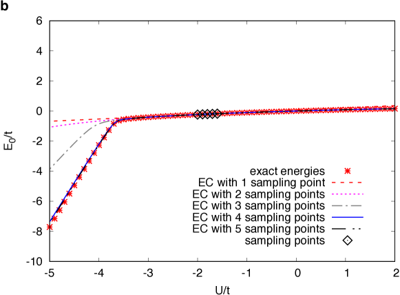
Figure 4.2: Ground state energy of the Bose-Hubbard model, done with up to 5th order eigenvector continuation (5 training vectors.)

To illustrate this, we consider 3rd order eigenvector continuation, in which we take three sampling points $U/t=-5.0,-1.5,2.0$. Using the ground state wavefunctions for each coupling, and using the procedure from Section 2.2, we can extract the EC estimate for $E_{0}$. This result is shown also in Fig. [4.1].

At first glance, it may appear as though we got lucky. After all, we sampled values of the coupling from each of the three ”physically-different” regions, so it seems obvious that an expansion using linear combinations of these three wavefunctions would cover the full range of couplings. However, we can sample couplings from entirely within one of the regions, say from the region $U/t=-2.0$ to$-1.6$. If we now consider eigenvector continuation with up to 5 vectors, from the couplings $U/t=-2.0,-1.9,-1.8,-1.7,-1.6$, we get the results in Fig. [4.2]. We see that even in this case, at high enough order, the EC result is able to capture the kink in $E_{0}$ at the point $U/t\approx-3.8$.

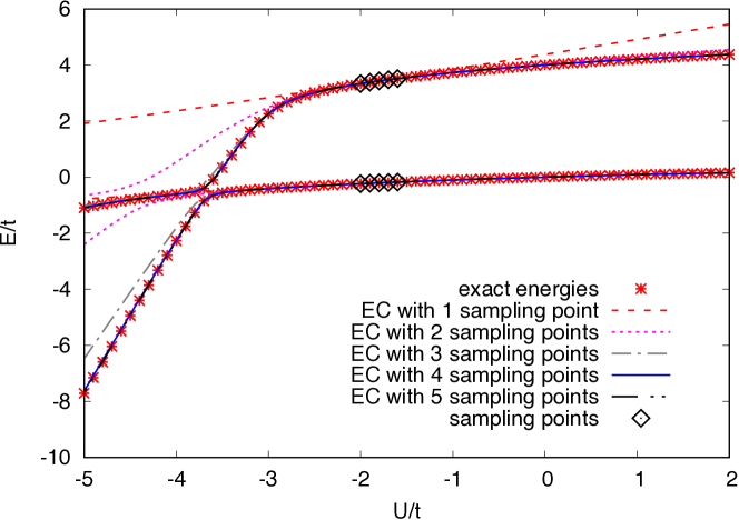
Figure 4.3: Computation of the lowest two energies in the Bose-Hubbard model. Here, the lowest two eigenvectors at each training coupling were kept and used to construct the EC subspace.

In Section 3.1, we discussed how including multiple eigenvectors at each sampling point can accelerate the convergence of the EC results. To demonstrate this, we now wish to compute the two lowest, even-parity states of the Bose-Hubbard system. These results are shown in Fig. [4.3]. We can now clearly see the avoided level crossing. The couplings used are still $U/t=-2.0,-1.9,-1.8,-1.7,-1.6$, however, we now take the two lowest eigenvectors at each value for the coupling, and use these to form our EC subspace. Comparing with the results of only including one vector per sampling point, we see that the convergence has been improved; the third order result is much closer, and the fourth/fifth order results are in quite good agreement with the exact energies.

4.2 Simulations of Neutron Matter

The second system we studied was the system of pure neutron matter. The objective was to demonstrate the use of eigenvector continuation to a full many-body Quantum Monte Carlo simulation. We considered systems of six or fourteen neutrons at leading order (LO) in chiral effective field theory. While there exist computationally-friendly lattice actions, as described in [18, 19], the more demanding lattice action [33] was instead chosen to serve as a better test for the method.

Since we are considering only neutrons, we can simplify the lattice action by reducing the number of independent contact interactions from two to one. In the following equations, we use $a_{i}\left(\textbf{n}\right)$ and $a^{\dagger}_{i}\left(\textbf{n}\right)$ to denote the fermion annihilation and creation operators, with spin component $i$ located at the lattice site n. We use the shorthand $a\left(\textbf{n}\right)$ and $a^{\dagger}\left(\textbf{n}\right)$ to denote the column vector of nucleon components and row vector of nucleon components, respectively. We use a spatial lattice spacing of $a$ = 1/100 MeV^-1 = 1.97 fm, and a temporal lattice spacing of $a_{t}$ = 1/150 MeV^-1 = 1.32 fm. We also set $\hbar=c=1$.

Our free, non-relativistic lattice Hamiltonian is given by

$$H_{\text{free}}\left(a^{\dagger},a\right)=\sum_{k=0,1}\frac{\left(-1\right)^{k}}{2m}\sum_{\textbf{n}}\sum_{l=1,2,3}a^{\dagger}\left(\textbf{n}\right)\left[a\left(\textbf{n}+k\hat{\textbf{l}}\right)+a\left(\textbf{n}-k\hat{\textbf{l}}\right)\right]$$ (4.2)

where $\hat{\textbf{l}}=\hat{\textbf{1}},\hat{\textbf{2}},\hat{\textbf{3}}$ denote the three spatial lattice unit vectors. The nucleon mass $m$ is taken to be 938.92 MeV.

We use the auxiliary field formalism to include the interactions between the neutrons. We then express the Euclidean time-evolution operator over $L_{t}$ time steps as a product of transfer matrix operators which depend on the auxiliary field $s$ and the pion field $\pi_{0}$.

$$U\left(L_{t},g_{A}^{2}\right)=\int DsD\pi_{0}\exp\left[-\mathcal{S}_{SS}\left(s\right)-\mathcal{S}_{\pi_{0}\pi_{0}}\left(\pi_{0}\right)\right]\left\{M^{\left(L_{t}-1\right)}\cdots M^{\left(0\right)}\right\}$$ (4.3)

For convenience, we have explicitly listed the dependence of this operator on the square of the axial vector coupling $g_{A}^{2}$. The quadratic part of the auxiliary field action is

$$\mathcal{S}_{SS}\left(s\right)=\frac{1}{2}\sum_{\textbf{n},n_{t}}s^{2}\left(\textbf{n},n_{t}\right)$$ (4.4)

and the quadratic part of the pion field action is

$$\mathcal{S}_{\pi_{0}\pi_{0}}\left(\pi_{0}\right) =\frac{1}{2}\alpha_{t}m_{\pi}^{2}\sum_{\textbf{n},n_{t}}\pi_{0}^{2}\left(\textbf{n},n_{t}\right)$$ (4.5)

$$+\frac{1}{2}\alpha_{t}\sum_{k=0,1}\left(-1\right)^{k}\sum_{\textbf{n},n_{t}}\sum_{l=1,2,3}\pi_{0}\left(\textbf{n},n_{t}\right)\left[\pi_{0}(\textbf{n}+k\hat{\textbf{l}},n_{t})+\pi_{0}(\textbf{n}-k\hat{\textbf{l}},n_{t})\right]$$ (4.6)

with the pion mass $m_{\pi}$ is taken to be 134.98 MeV.

The normal-ordered auxiliary field transfer matrix, for a given time step $n_{t}$, is given by

$$M^{\left(n_{t}\right)}=:\exp\left[-H^{\left(n_{t}\right)}(a^{\dagger},a,s,\pi_{0})\alpha_{t}\right]:$$ (4.7)

The Hamiltonian at the time step $n_{t}$ is given by

$$H^{\left(n_{t}\right)}(a^{\dagger},a,s,\pi_{0})\alpha_{t}=H_{\text{free}}\left(a^{\dagger},a\right)\alpha_{t}+S_{s}^{\left(n_{t}\right)}\left(a^{\dagger},a,s\right)+S_{\pi_{0}}^{\left(n_{t}\right)}\left(a^{\dagger},a,\pi_{0}\right)$$ (4.8)

where

$$S_{s}^{\left(n_{t}\right)}(a^{\dagger},a,s)=\sqrt{-C\alpha_{t}}\sum_{\textbf{n}}s(\textbf{n},n_{t})a^{\dagger}(\textbf{n})a(\textbf{n})$$ (4.9)

$$S_{\pi_{0}}^{\left(n_{t}\right)}(a^{\dagger},a,\pi_{0})=\frac{g_{A}\alpha_{t}}{2f_{\pi}}\sum_{\textbf{n}}\sum_{l=1,2,3}\frac{1}{2}[\pi_{0}(\textbf{n}+k\hat{\textbf{l}},n_{t})+\pi_{0}(\textbf{n}-k\hat{\textbf{l}},n_{t})]a^{\dagger}(\textbf{n})\sigma_{l}a(\textbf{n})$$ (4.10)

Here, C is the coupling of the contact interaction, and is taken to be $-4.5\times 10^{-5}$ MeV^-2. This is different from the value used in [33]; however, this value was chosen to reproduce a more realistic equation of state for neutron matter at the densities being probed in our simulations. $\sigma_{l}$ denote the Pauli spin matrices. $f_{\pi}$ is the pion decay constant, which we take to be 92.2 MeV. $g_{A}$ is the axial-vector coupling, taken as 1.29. After integrating over the pion fields, we obtain a one-pion exchange potential that is quadratic in $g_{A}$.

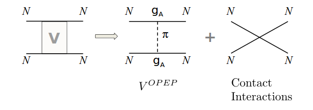
Figure 4.4: LO chiral forces used in neutron matter simulations. Included interactions include a contact term and one-pion exchange

We performed simulations of six and fourteen neutrons in a 4³ box, extracting the ground state wavefunctions. In physical units, L = 7.9 fm, and the corresponding number densities are 0.012 fm³ for six neutrons and 0.028 fm³ for fourteen neutrons. Our initial and final states are taken as free Fermi gas wavefunctions, which we denote $|\Phi\rangle$. We use Euclidean time projection to produce the ground states for given values of $g_{A}^{2}$, which we denote $|\Phi,n_{t},g_{A}^{2}\rangle$.

$$|\Phi,n_{t},g_{A}^{2}\rangle=U\left(n_{t},g_{A}^{2}\right)|\Phi\rangle$$ (4.11)

For large $n_{t}$, $|\Phi,n_{t},g_{A}^{2}\rangle$ will asymptotically approach the ground state.

First, we present the results of direct calculation without eigenvector continuation. In these calculations, we perform Monte Carlo simulations for the pion and auxiliary fields, and calculate the ratio

$$r\left(L_{t}\right)=\frac{\langle\Phi|U\left(L_{t},g_{A}^{2}\right)|\Phi\rangle}{\langle\Phi|U\left(L_{t}-1,g_{A}^{2}\right)|\Phi\rangle}$$ (4.12)

in the large $L_{t}$ limit. This ratio is converted into an energy by

$$E(L_{t})=-\log\{r(L_{t})\}/a_{t}\approx E_{0}+ce^{-\delta EL_{t}a_{t}}$$ (4.13)

In Fig. [4.5], we show the direct result for the calculation of six neutrons. The red open squares show the lattice results versus projection time, including the one-$\sigma$ error bars reflecting the stochastic errors in the simulation. From the asymptotic form in Eqn. [4.13], the best fit is shown as a red, solid line, and the limits of the one-standard-deviation error bars are shown as red dashed lines. In Fig. [4.6], we show the results of the direct calculation for fourteen neutrons. The red open squares show the lattice results versus projection time, including one-standard-deviation error bars indicating stochastic errors. The best fit is shown as a red solid line, and the limits of the one-standard-deviation error bands are shown as red dashed lines. Due to large sign oscillations, it is not possible to do simulations at large projection times. This is reflected in the large uncertainties of the ground state energy extrapolations.

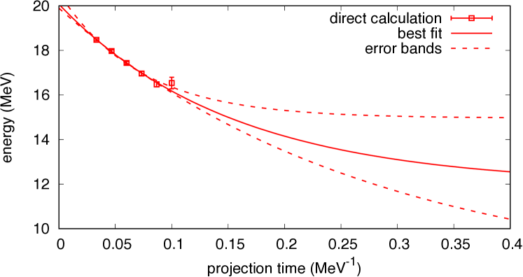
Figure 4.5: Direct calculation of the ground state energy for six neutrons, shown as a function of Euclidean time. The red, open squares are the lattice results, and the solid red line is the best fit showing the exponential decay of the signal. The dashed red line is the 1$\sigma$ error band for the fit.

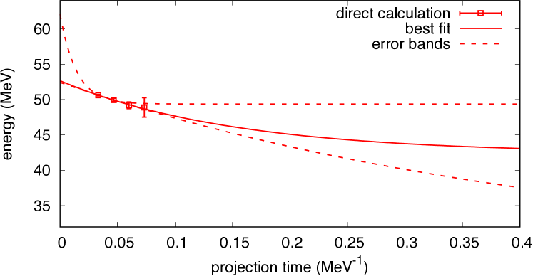
Figure 4.6: Direct calculation of the ground state energy for fourteen neutrons, shown as a function of Euclidean time. The red, open squares are the lattice results, and the solid red line is the best fit showing the exponential decay of the signal. The dashed red line is the 1$\sigma$ error band for the fit.

For the eigenvector continuation, we compute the inner products

$$N_{i,i^{\prime}}(n_{t})=\langle\Phi,n_{t},c_{i}^{\prime}|\Phi,n_{t},c_{i}\rangle$$ (4.14)

for sampling values $g_{A}^{2}=c_{1},c_{2},c_{3}$, where $c_{1}=0.25$, $c_{2}=0.60$, and $c_{3}=0.95$. We also calculate the matrix elements of the full transfer matrix for the target value $c_{\odot}=1.29^{2}=1.66$,

$$M_{i,i^{\prime}}(n_{t})=\langle\Phi,n_{t},c_{i}^{\prime}|U(1,c_{\odot})|\Phi,n_{t},c_{i}\rangle$$ (4.15)

To extract the EC energy, we solve the generalized eigenvalue problem $N^{-1/2}MN^{-1/2}$, finding the largest eigenvalue $\lambda(n_{t})$, and using the relation

$$E(n_{t})=-\log\{\lambda(n_{t})\}/a_{t}\approx E_{0}+ce^{-\delta E(2n_{t}+1)a_{t}}$$ (4.16)

In these calculations, we consider seven different choices for the EC subspace. For the first three, we consider the 1-D subspaces formed by a single vector $|\Phi,n_{t},c_{i}\rangle$ for $i=1,2,3$. The next three consist of the 2-D subspaces formed by taking two vectors $|\Phi,n_{t},c_{i}\rangle$ and $|\Phi,n_{t},c_{i}^{\prime}\rangle$ for $i\neq i^{\prime}$. Lastly, we consider the full 3-D subspace formed from all three vectors.

The EC results for six neutrons are shown in Fig. [4.7]. The ground state energy is shown versus projection time using sampling data $g_{A}^{2}=c_{1},c_{2},c_{3}$, where $c_{1}=0.25$, $c_{2}=0.60$, and $c_{3}=0.95$. We show results for one, two and three vectors. The errors are estimated using a jackknife analysis of the Monte Carlo data. In order to decrease the sensitivity to stochastic noise, we have used a common $\delta E$ for all cases. We have also imposed a variational constraint that adding more vectors to the EC subspace will not increase the energy. The EC results for fourteen neutrons are shown in Fig. [4.8], with the same choices for $c_{1},c_{2},c_{3}$.

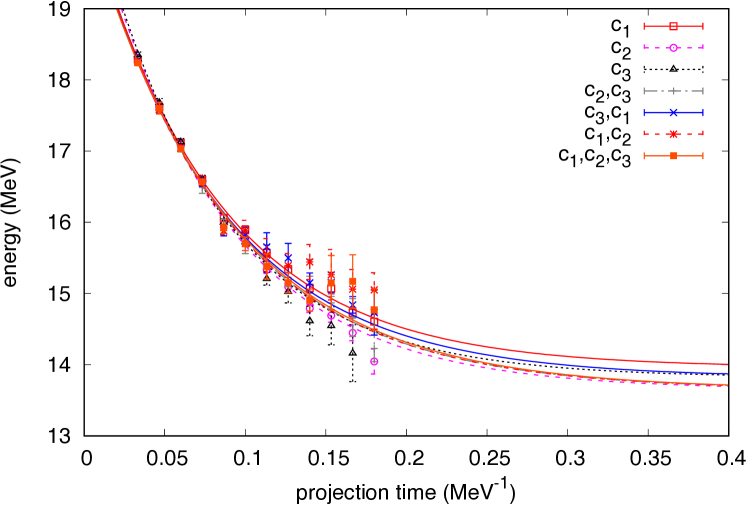
Figure 4.7: Eigenvector continuation results for six neutrons, including up to three vectors in the training subspace. Open squares show the EC estimates for the ground state energy for a particular set of vectors used to construct the subspace. The lines show the best fits of these results.

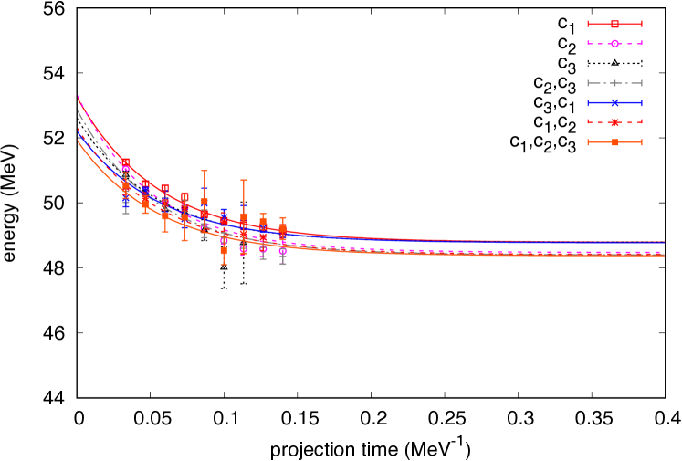
Figure 4.8: Eigenvector continuation results for fourteen neutrons, including up to three vectors in the training subspace. Open squares show the EC estimates for the ground state energy for a particular set of vectors used to construct the subspace. The lines show the best fits of these results.

We summarize all of the results in Table [4.1]. For reference, the nuclear densities present in each simulation are provided. These are computed by $\rho_{N}=N/V$, where $N$ is the number of neutrons in the box, and $V$ is the volume of the box, in units of fm^-3. In both cases, we see that the estimates for the error have improved by a factor of 10 to 20.

$g^{2}_{A}$ Values	$E_{0}$ for 6 neut. (MeV)	$E_{0}$ for 14 neut. (MeV)
$c_{1}$	13.8(1)	48.9(4)
$c_{2}$	13.6(2)	48.4(5)
$c_{3}$	13.6(2)	48.9(6)
$c_{2}$,$c_{3}$	13.6(2)	48.1(6)
$c_{3}$,$c_{1}$	13.6(2)	48.9(6)
$c_{1}$,$c_{2}$	13.6(2)	48.0(6)
$c_{1}$,$c_{2}$,$c_{3}$	13.6(2)	48.0(6)
direct calc.	12$\left({}^{+3}_{-4}\right)$	42$\left({}^{+7}_{-15}\right)$
$\rho_{N}$	0.012 fm-3	0.028 fm-3

Table 4.1: Summary of the neutron matter results, for 6 and 14 neutrons, compared to the direct Monte Carlo calculations. For reference, the relevant nuclear densities are provided.

4.3 Coulomb Interaction in ¹²C and ¹⁶O

The non-perturbative simulation of the Coulomb interaction in light nuclei is the main project described in this work. For most nuclear simulations, the Coulomb interaction is handled perturbatively. However, due to its repulsive nature, it leads to sign problems for all but the lightest nuclei.

We want to use eigenvector continuation to circumvent this problem, by adding the Coulomb interaction directly to the transfer matrix via auxiliary fields, and getting ground state wavefunctions for various couplings. Then, we can build the EC estimate for the energy shift due to the Coulomb interaction using the method described in Section 2.4.4.

On the lattice, the Coulomb interaction has the form

$$V(|\textbf{n}-\textbf{n}^{\prime}|)=\frac{\alpha_{em}}{\text{max}(0.5,|\textbf{n}-\textbf{n}^{\prime}|)}$$ (4.17)

where $\alpha_{e}m=1/137$ is the fine structure constant, and $|\textbf{n}-\textbf{n}^{\prime}$ is the distance between lattice sites. The denominator has the max function to prevent the potential taking an infinite value at zero distance. The value at the origin is chosen to be $V(0)=2\alpha_{em}$. While this approximation may seem incorrect, it doesn’t affect the p-p scattering phase shifts or any of the low-energy nuclear observables.

To add this interaction into the transfer matrix, we define a new auxiliary field $s_{1}$,

$$M(s,s_{1},t)=:\exp\{-H_{\text{free}}\alpha_{t}+\sqrt{-\alpha_{em}\alpha_{t}}\sum_{\vec{n}}s_{1}(\vec{n},n_{t})\rho(\vec{n},n_{t})\}:$$ (4.18)

where $H_{\text{free}}$ consists of the kinetic energy term, and $\rho(\vec{n},n_{t})$ is the density operator at the lattice site $(\vec{n},n_{t})$. The $s_{1}$ auxiliary field is pulled from the distribution

$$P=\exp\left(-\mathcal{S}\right)=\exp\left(-\sum_{\vec{n},\vec{n}^{\prime}}s_{1}(\vec{n},n_{t})V^{-1}(\vec{n}-\vec{n}^{\prime})s_{1}(\vec{n}^{\prime},n_{t})\right)$$ (4.19)

following the prescription in section 2.4.4.

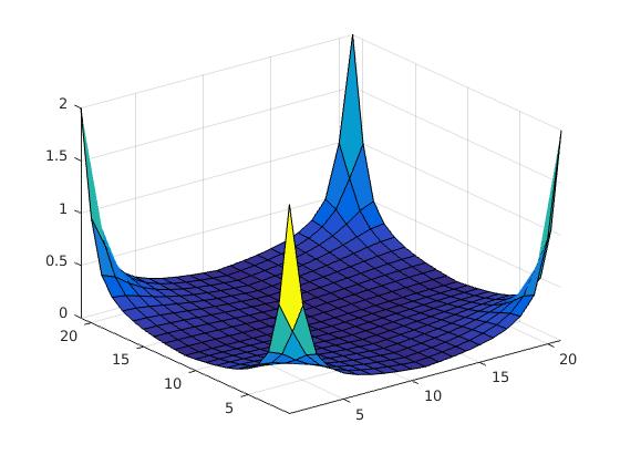
Figure 4.9: Values of the Coulomb potential on the $n_{z}$=0 plane. The value at the origin is chosen to be $V(0)=2\alpha_{em}$. This is large enough to give good results.

This calculation was implemented in the MCLEFT code [51], which uses the shuttle algorithm to update the auxiliary fields and propagate the wavefunctions using the transfer matrices. Two new modules were written, eigenvectorContinuation and eigenvectorContinutationAuxiliary, which were designed to compute the ground state wavefunctions for various couplings for this $s_{1}$ field. Then, the eigenvector continuation technique could be applied using the interactions in the MCLEFT code as a baseline. Also, the MCLEFT code calculates the Coulomb energy perturbatively, so that was used as a benchmark for the method.

We start with ¹²C, computed on an $L=5$ lattice, with lattice spacings of $a=1/100$ $\text{ MeV}^{-1}$ and $a_{t}=1/1000\text{ MeV}^{-1}$. We first motivate the need for the eigenvector continuation technique, by looking at the ground state energy of ¹²C with Coulomb included via direct calculation. The Coulomb interaction has a noticeable sign problem in larger nuclei, so we tune the fine structure constant to be four times its physical value, $C_{\odot}=4\alpha_{em}$. Results for this is shown in Fig. [4.10].

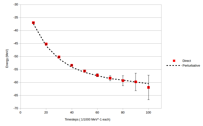
Figure 4.10: Direct calculation of Coulomb energy shifts for ¹²C, at $C_{\odot}=4\alpha_{em}$. The black dotted line shows the perturbative results, and the orange squares show the results of the direct calculation. We see that for large projection times the sign problem begins to show up, before we have reached a proper plateau.

We use perturbative results as a reference value. In general, perturbative results will not be available, or if they are, they may not be reliable. In the case of the Coulomb interaction, perturbation theory works well enough to estimate the energy that it can be used as a benchmark. These are shown with the black dotted line.

Ideally, we would compute this energy for several projection times, and show a nice exponential decay that we could fit the true, infinite projection time ground state energy to. However, we see the rapid onset of the Monte Carlo sign problem, which causes large oscillations in the amplitudes at large projection time. This causes the statistical errors to explode, making large $\tau$ extrapolations virtually impossible.

Like we did for the neutron matter system, we turn to eigenvector continuation to save us. We can take a set of wavefunctions for small couplings, small enough that the sign problem doesn’t bother us, and use them to extrapolate to couplings that would be otherwise inaccessible.

We now show the results of this EC calculation for ¹²C, up to 3rd order. The couplings used in the EC subspace are $C_{EC}=0\alpha_{em},2.0\alpha_{em},\text{ and }4.0\alpha_{em}$, and the target coupling is $C_{\odot}=4\alpha_{em}$. This is the same target coupling used in the direct calculation, so that we can easily compare the accuracy and stability of the results. These EC results are plotted in Fig. [4.11].

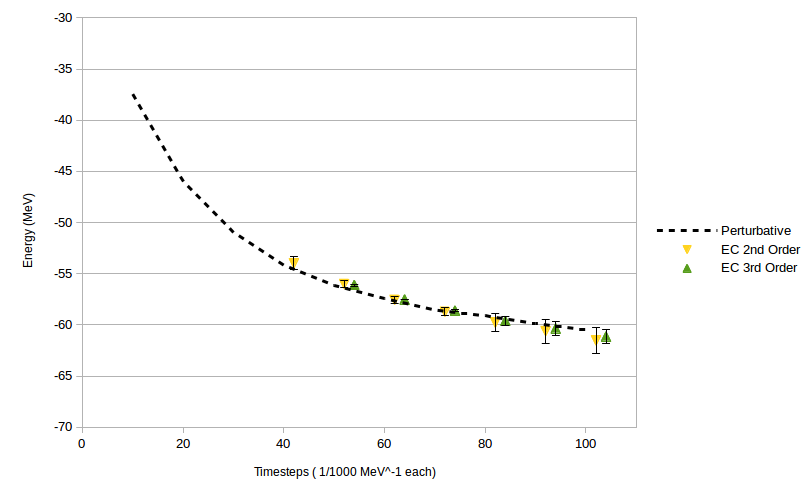
Figure 4.11: EC Calculation of Coulomb energy shifts in ¹²C. Again, we show the perturbative results as a reference. Early on, the EC norm matrix is very singular, so data is not present before $L_{t}=40$. We note that the 2nd and 3rd order results are computed at the same projection times; they are only separated on the plot for visual clarity.

In yellow, we show the 2nd order results, computed using the wavefunctions at coupling $C_{EC}=2.0\alpha_{em},\text{ and }4.0\alpha_{em}$. In green are the 3rd order results, computed with the wavefunctions at all three couplings $C_{EC}=0\alpha_{em},2.0\alpha_{em},\text{ and }4.0\alpha_{em}$. For small projection times, we ran into numerical instability in the norm matrix. This is due to the fact that all the wavefunctions start in the same initial state; thus, for small projection times, the wavefunctions haven’t gotten the chance to change much. It takes until $L_{t}=40$ ($\tau=7.88\text{ fm}$) for the 2nd order results to become stable, and $L_{t}=50$ ($\tau=9.85\text{ fm}$) for the 3rd order results to become stable. We now show these two sets of data on the same plot, in Fig. [4.12], to better compare the methods. The values on this plot are summarized in Table [4.2].

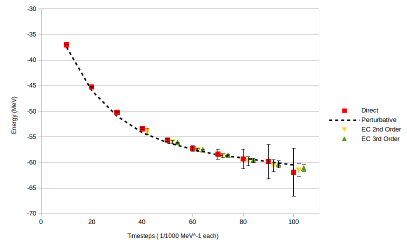
Figure 4.12: Combined plot showing the direct results and the EC estimates of Coulomb energy shifts in ¹²C. We can immediately see the improvement gained by the EC method, and the overall resilience to the sign problem. We note that the three points in each pack are computed at the same projection times; they are only separated on the plot for visual clarity.

Timesteps	$\tau$ (fm)	Perturbative	Direct Calc.	2nd Order EC	3rd Order EC
10	1.97	-37.448(51)	-37.012(20)	-	-
20	3.94	-45.964(52)	-45.239(43)	-	-
30	5.91	-50.934(59)	-50.209(100)	-	-
40	7.88	-54.164(63)	-53.435(177)	-53.982(633)	-
50	9.85	-56.138(77)	-55.648(335)	-56.002(376)	-56.111(95)
60	11.82	-57.428(72)	-57.268(571)	-57.553(321)	-57.515(45)
70	13.79	-58.546(84)	-58.397(936)	-58.716(398)	-58.606(130)
80	15.76	-59.120(99)	-59.341(1900)	-59.788(897)	-59.613(474)
90	17.73	-59.872(105)	-59.814(3352)	-60.601(1169)	-60.343(680)
100	19.70	-60.490(99)	-61.944(4708)	-61.527(1316)	-61.133(686)

Table 4.2: Summary of the Coulomb results in ¹²C, computed via direct calculation, and by eigenvector continuation. Dashed entries are where a singular norm matrix prevented stable calculations.

In Section 3.2, we mentioned that it is often easier to break the computation of the EC inserted operator matrix $M$ into two pieces

$$M=M_{0}+C_{\odot}M_{EC}$$ (4.20)

so that we could perform the eigenvector simulations in the post-processing stage, for arbitrary target coupling.

In Fig. [4.13], we show the results of tuning the target Coulomb strength $C_{\odot}=x\alpha_{em}$ in the range $0.0<x<10.0$. We show the perturbative results again as a reference. Using perturbation theory, we expect this energy correction to be linear in the coupling $E_{0}\propto\alpha_{em}$. Thus, any deviations from this would be hints of higher-order terms.

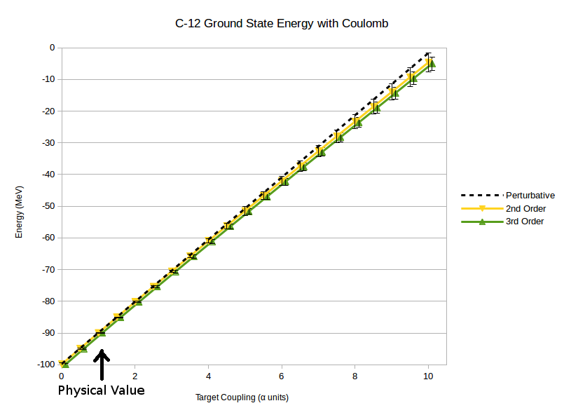
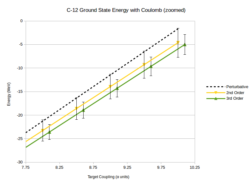
Figure 4.13: Computation of Coulomb energy shifts in ¹²C for arbitrary target coupling. $C_{\odot}$ was varied in the range $0.0\alpha_{em}\leq C_{\odot}\leq 10.0\alpha_{em}$. Shown in the bottom figure is a zoom of larger coupling region, showing a clear deviation from the perturbative results.

We now show a few other tests that we performed to check the validity of the simulations. In Fig [4.14], we show the convergence of the ¹²C EC ground state energy estimate as a function of the Monte Carlo step. This is a test any Monte Carlo calculation should check first; a good result should be converged after a suitably large number of trials. We see that here; after 7,000 steps or so, the result doesn’t vary much, and the error estimate from the Online algorithm seems to be approaching a steady value.

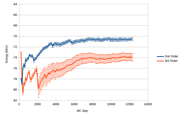
Figure 4.14: Plot of the EC estimate for the ground state energy of ¹²C, as a function of the MC step. Shown are also the 1$\sigma$ error bars at each step. These calculations were done at a target coupling $C_{\odot}=3\alpha_{\text{em}}$. We see that after  7000 steps, the results are more-or-less converged, though the 3rd order results experience some numerical instability.

We now move on to simulations of ¹⁶O. Here, the number of particles is starting to get high enough that simulations at large projection times become even more problematic. In Figs. [4.15 - 4.17], we show plots like the ¹²C plots; the results from direct calculation of the Coulomb energy shifts, and a result for performing the eigenvector continuation method. We see that for large projection times, the sign problem once again kills us, though, it is much more sever this time around. Also, the use of the eigenvector continuation has not only stabilized the results, but has also reduced the errors rather dramatically. The values on these plots are summarized in Table [4.3].

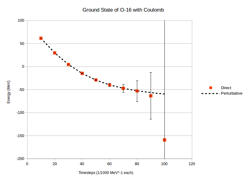
Figure 4.15: Direct calculation of Coulomb energy shifts for ¹⁶O

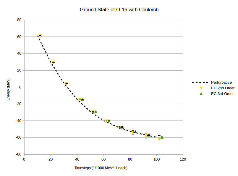
Figure 4.16: EC Calculation of Coulomb energy shifts in ¹⁶O. For $L_{t}=10-30$, the 3rd order results were too unstable to extract reliable data.

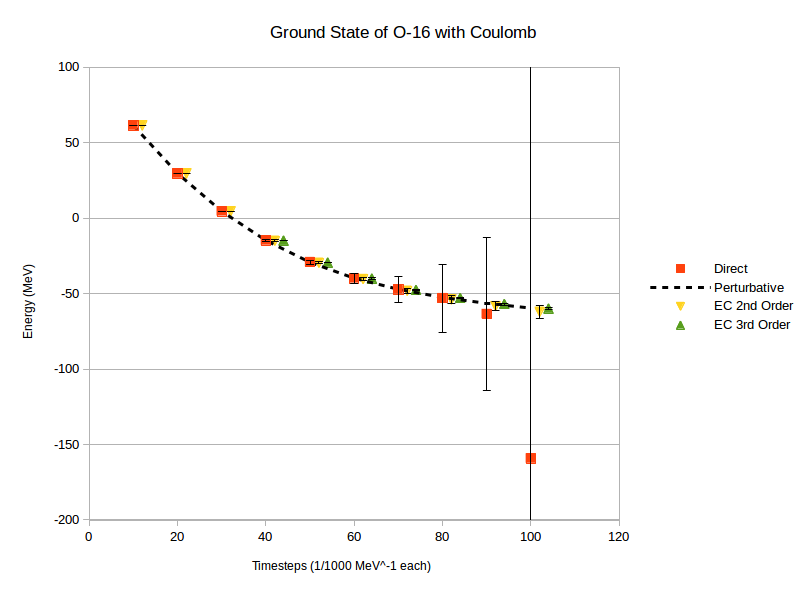
Figure 4.17: Combined plot showing the direct results and the EC estimates of Coulomb energy shifts in ¹⁶O.

Timesteps	$\tau$ (fm)	Perturbative	Direct Calc.	2nd Order EC	3rd Order EC
10	1.97	61.406(89)	61.408(28)	61.35(18)	-
20	3.94	29.60(10)	29.579(73)	29.51(19)	-
30	5.91	4.53(10)	4.54(17)	4.43(28)	-
40	7.88	-14.81(12)	-14.74(50)	-14.94(48)	-14.87(17)
50	9.85	-29.31(12)	-29.12(125)	-29.56(69)	-29.43(18)
60	11.82	-39.82(13)	-39.93(346)	-40.34(113)	-40.02(38)
70	13.79	-47.16(13)	-47.25(833)	-48.11(167)	-47.59(49)
80	15.76	-52.54(15)	-53.02(2254)	-53.92(236)	-52.98(58)
90	17.73	-56.44(15)	-63.55(5091)	-58.35(302)	-57.00(66)
100	19.70	-59.60(15)	-159.27(426912)	-62.04(446)	-56.96(83)

Table 4.3: Summary of the Coulomb results in ¹⁶O, computed via direct calculation, and by eigenvector continuation. Dashed entries are where a singular norm matrix prevented stable calculations.

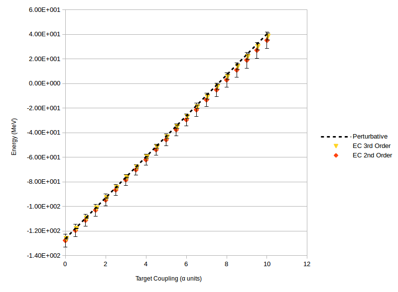
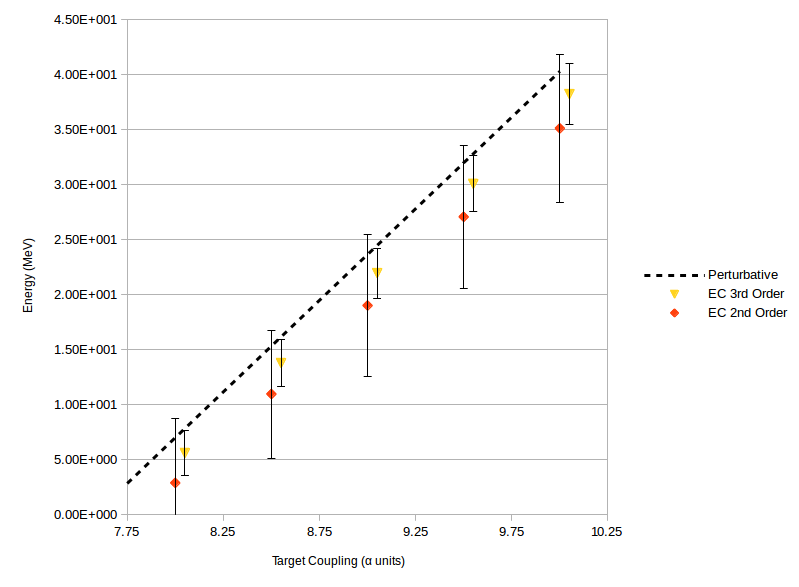
Figure 4.18: Computation of Coulomb energy shifts in ¹⁶O for arbitrary target coupling. $C_{\odot}$ was varied in the range $0.0\alpha_{em}\leq C_{\odot}\leq 10.0\alpha_{em}$. Shown in the bottom figure is a zoom of larger coupling region.

We now repeat the same consistency checks that we performed for the ¹²C simulations. In Fig. [4.19], we show the convergence of the ¹⁶O EC ground state energy estimate as a function of the Monte Carlo step. It takes a bit longer to reach a stable value, but it does appear to be converged.

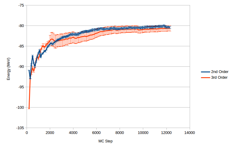
Figure 4.19: Plot of the EC estimate for the ground state energy of ¹⁶O, as a function of the MC step. Shown are also the 1$\sigma$ error bars at each step. These calculations were done at a target coupling $C_{\odot}=3\alpha_{\text{em}}$.

4.4 EC Solutions of the Lipkin Hamiltonian

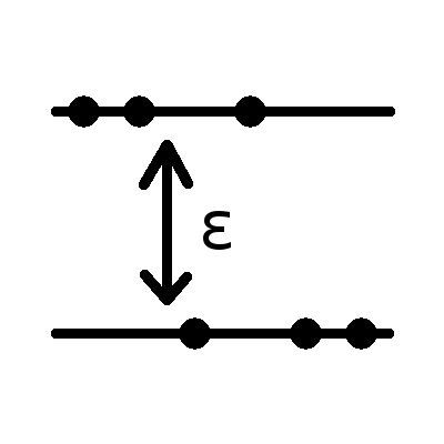
Figure 4.20: Basic schematic of the Lipkin model. There are N particles distributed among two angular momentum levels, $m=\pm 1/2$, separated by some gap $\epsilon$.

The Lipkin-Meshkov-Glick (or just Lipkin) model [50] is a model that was developed to test many-body approximation methods and numerical techniques. It was designed to both be exactly solvable, yet to have non-trivial behaviour.

The model consists of N fermions distributed between two levels, each assumed to be N-fold degenerate. Each particle is assumed to be spin-1/2, and the overall wavefunction $|J,m\rangle$ is given by a total angular momentum $J$ and projection of the angular momentum onto the z-axis $m$. The interaction is written in terms of angular momentum operators

$$H=\epsilon J_{z}+\frac{V}{2}(J_{+}^{2}+J_{-}^{2})+\frac{W}{2}(J_{+}J_{-}+J_{-}J_{+})$$ (4.21)

where $J_{z}$, $J_{+}$ and $J_{-}$ act according to ($\hbar=1$)

$$J_{z}|J,m\rangle =m|J,m\rangle$$

$$J_{+}|J,m\rangle =\sqrt{J(J+1)-m(m+1)}|J,m+1\rangle$$ (4.22)

$$J_{-}|J,m\rangle =\sqrt{J(J+1)-m(m-1)}|J,m-1\rangle$$

The first term is a count of the single particle energies, while the second and third term are what leads to interesting behaviours. The second term, or the V term, is responsible for moving two particles from one level to the other, thus changing m by two units. The third term, or the W term, allows swapping an upper-level particle and a lower-level particle.

This terms that allow mixing are responsible for a quantum phase transition. This feature of the Lipkin model has been well-studied [5] [69] [10] [72] [67] [34], and has been used as a testing ground for studying these phase transitions.

While the dimension of this problem may seem large, we note that none of the operators in the Hamiltonian actually change $J$. This means the Hamiltonian matrix will be block diagonal. There will be $J_{\text{max}}=N/2$ blocks, one per value of $J$, and each block will be dimension $2J+1$, corresponding with the values of $m$. In this paper, we will only consider the $(N+1)\times(N+1)$ sub-matrix corresponding with $J=J_{\text{max}}$.

The first thing that was checked was how well perturbation theory worked in this model. For this, we used a Matlab code, developed by A. Sarkar (publication in the works). Results for these are shown in Figs. [4.21] and [4.22].

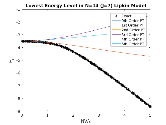
Figure 4.21: Results of the N=14 particle system using perturbation theory, up to 5th order. It is clear that perturbation theory diverges quickly for couplings far from 0.

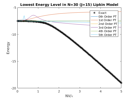
Figure 4.22: Results of the N=30 particle system using perturbation theory, up to 5th order. Convergence here is worse than the 14 particle system.

We now demonstrate the use of the eigenvector continuation technique to this model. Using a short Matlab code, we computed the first five eigenvectors of the Lipkin Hamiltonian, treating $V$ as our tunable parameter, for five different values of V; $V=0.1,0.2,0.3,0.4,0.5$. For now, we take $W=0$.

In each order of EC, which we call $\mu$, we formed a projection operator by taking the span of the first five eigenvectors for $\mu$ of the couplings, resulting in a $5\mu$-dimensional operator. Then, we projected the Hamiltonian $H(V^{\prime})$ into this subspace, resulting in a new matrix $\tilde{H}$. We then diagonalized $\tilde{H}$; the lowest 5 eigenvalues of this matrix we call the $\mu$-th order EC estimates.

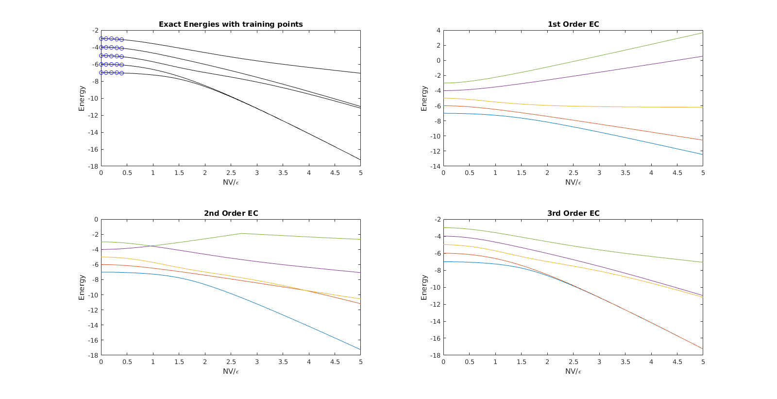
Figure 4.23: EC Estimates of the five lowest energy levels of the N=14 Lipkin model. The exact energies, obtained via diagonalizing $H$, are shown on the top left. At first order and second order, the estimates are not great, but the third order estimate (and beyond) are extremely good.

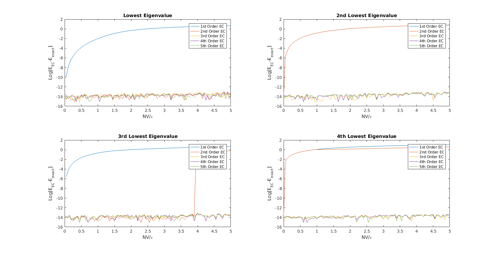
Figure 4.24: Error between the EC estimates and the exact eigenvalues for N=14 Lipkin model, shown on a log scale. The four lowest eigenvalues are shown, each calculated up to 5th order. $10^{-14}$ is about the machine level of precision, so better errors could be obtained by increasing precision.

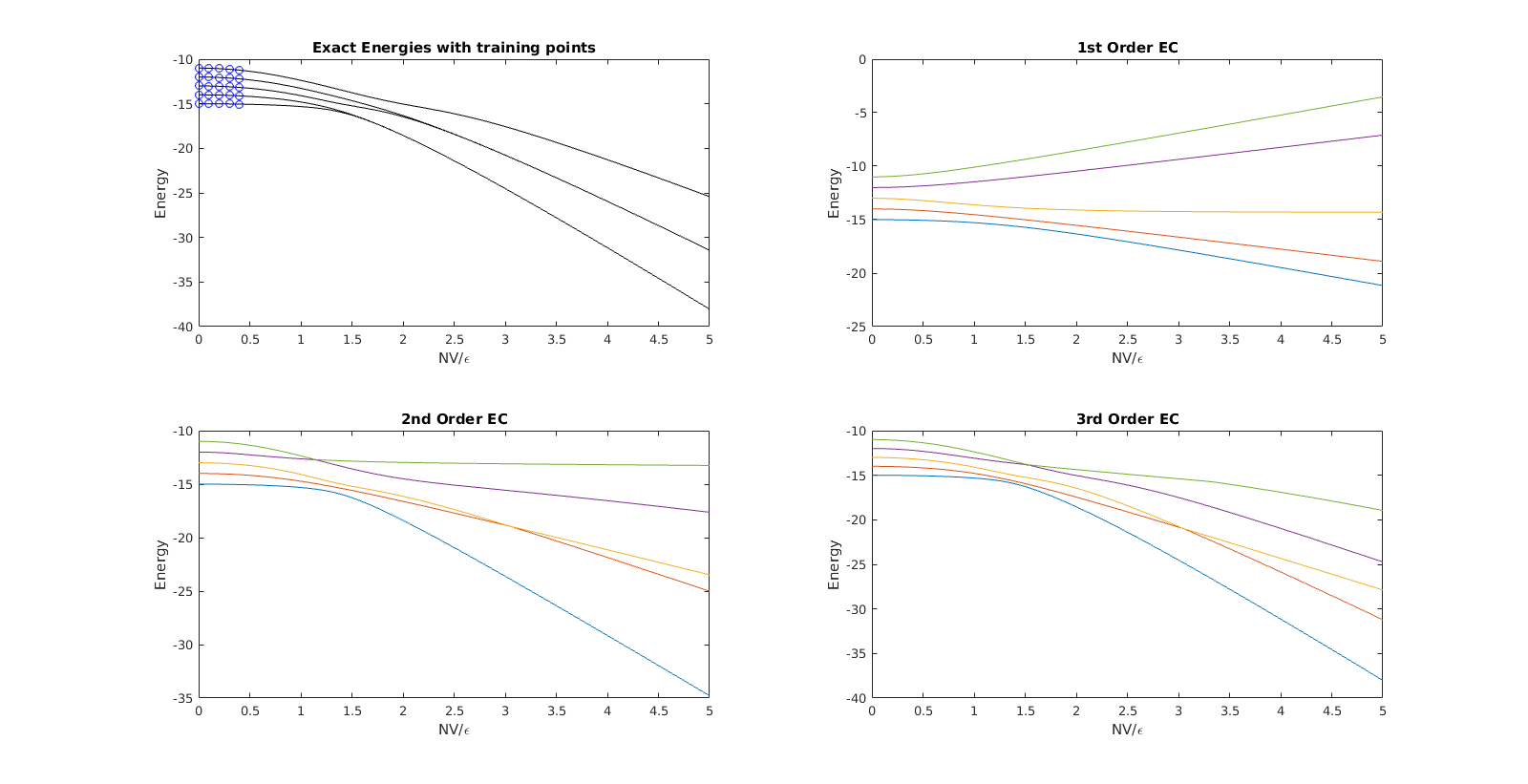
Figure 4.25: EC Estimates of the five lowest energy levels of the N=30 Lipkin model. The exact energies, obtained via diagonalizing $H$, are shown on the top left. The results converge much more slowly, and the improvements at higher orders are noticeable.

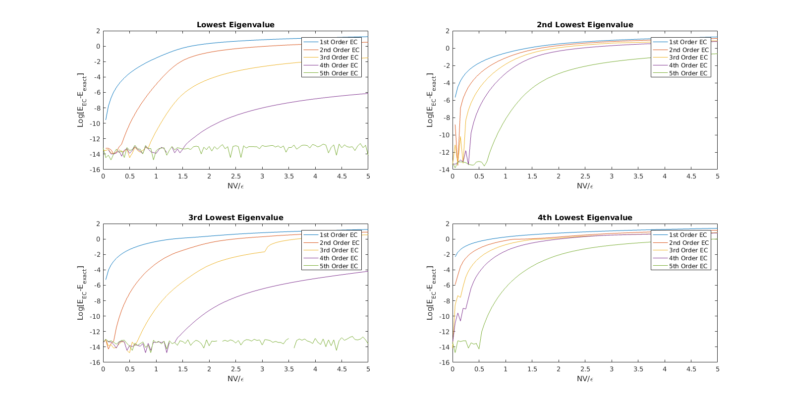
Figure 4.26: Error between the EC estimates and the exact eigenvalues for N=30 Lipkin model, shown on a log scale. The four lowest eigenvalues are shown, each calculated up to 5th order. The order-by-order convergence is more pronounced with this larger number of particles.

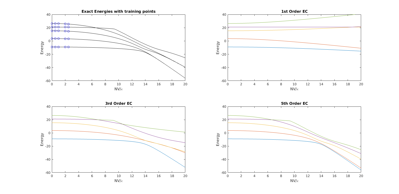
Figure 4.27: EC Estimates of the five lowest energy levels of the N=30 Lipkin model, with $W=0.4$. The exact energies, obtained via diagonalizing $H$, are shown on the top left. The 1st, 3rd, and 5th order results are shown, because convergence is overall slower than the results from $W=0$

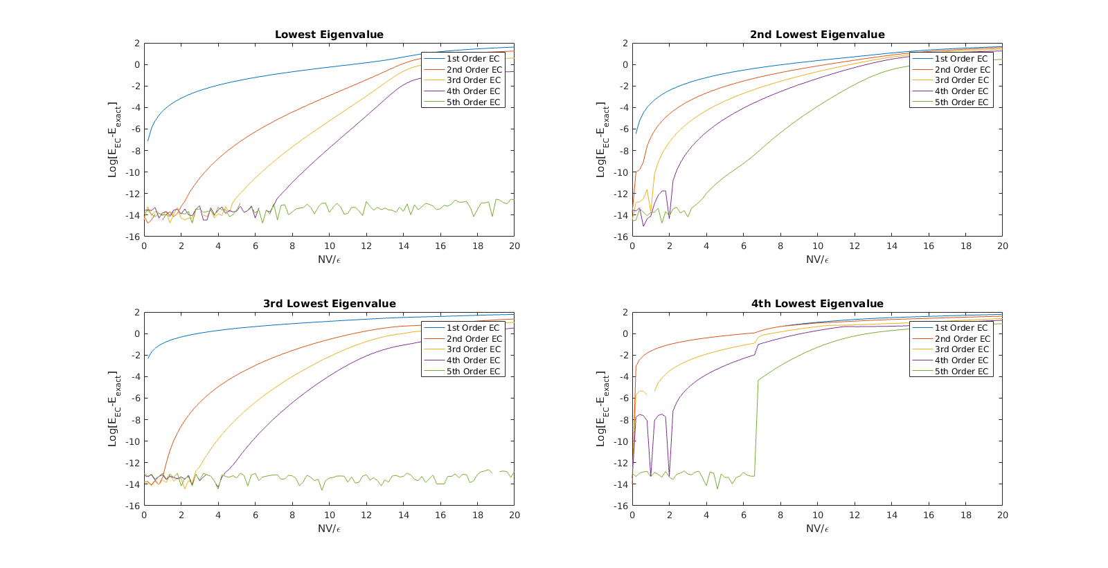
Figure 4.28: Error between the EC estimates and the exact eigenvalues for N=30 Lipkin model, with W = 0.4, shown on a log scale. The four lowest eigenvalues are shown, each calculated up to 5th order. While the residuals are larger, the order-by-order convergence is still present.

In Figures [4.23] and [4.25], we show the results of these calculations. We show for reference the exact energies, shown by the solid black lines in the top-left plot. On this top-left plot, we also show the points that were used in the construction of the EC subspace. The other three plots on each figure show the 1st, 2nd, and 3rd order results of the EC method. We see that while the 1st and 2nd order results are close for couplings near the training region, they tend to not behave for other couplings. However, when we reach 3rd order, we see almost perfect agreement, down to the level of precision in the calculation. We computed the 4th and 5th order estimates for the energies, but did not bother to plot them because we had already reached the numerical precision threshold.

To illustrate this agreement better, we show the residuals between the EC estimates for the energy and the exact values

$$R=\log_{10}\left(|E_{j,\text{EC}}-E_{j,\text{exact}}|\right)$$ (4.23)

plotted in Figures [4.24] and [4.26]. These are organized by eigenvalue, to show the order-by-order convergence in the results. $10^{-14}$ is as good as Matlab can do by default, so this put a limit on how accurately our results could be. For the $N=14$ system, the convergence was already below the machine threshold by the third order calculations. For the $N=30$ system, these errors were much larger, allowing us to see the improvements in each order of EC.

Now, to really test the method, we turn the W term on, taking a value of $W=0.4$. This leads to a more interesting energy level spectrum, with level crossings and the like. We still consider $N=30$. In Fig. [4.27], we show the first five eigenvalues, at first, third, and fifth order in EC. This is because the convergence isn’t as quick as before. Looking at the residuals, shown in Fig. [4.28], it is clear that the fifth order results are not quite converged enough.

Having demonstrated that the EC technique works, we will now push it to the strong coupling or large $N$ limit. Looking at the exact spectrum, we see a very tight pinch on the spectrum around $C=1.0$. This is signalling a branch point is very close to the real axis, which would cause the convergence of the EC method to dramatically slow down (if it works at all.)

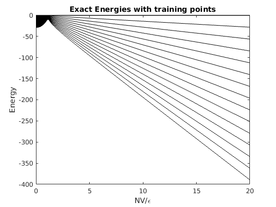
Figure 4.29: Plotted here are the first 20 energy levels for the N=1000 Lipkin Model. Due to the overall energy scale, we have subtracted out the lowest energy level. We note that the energy levels pinch together at around $C=1.0$, suggesting a nearby branch point.

We now apply the EC method, up to 15th order, to this system. In Figs. [4.30] and [4.31], we show the odd EC estimates (1st order to 11th order) for the first five eigenvalues, with the lowest eigenvalues subtracted out. On the top-left of each, we show the exact spectrum, with the lowest eigenvalue also subtracted out, and the training points in blue circles.

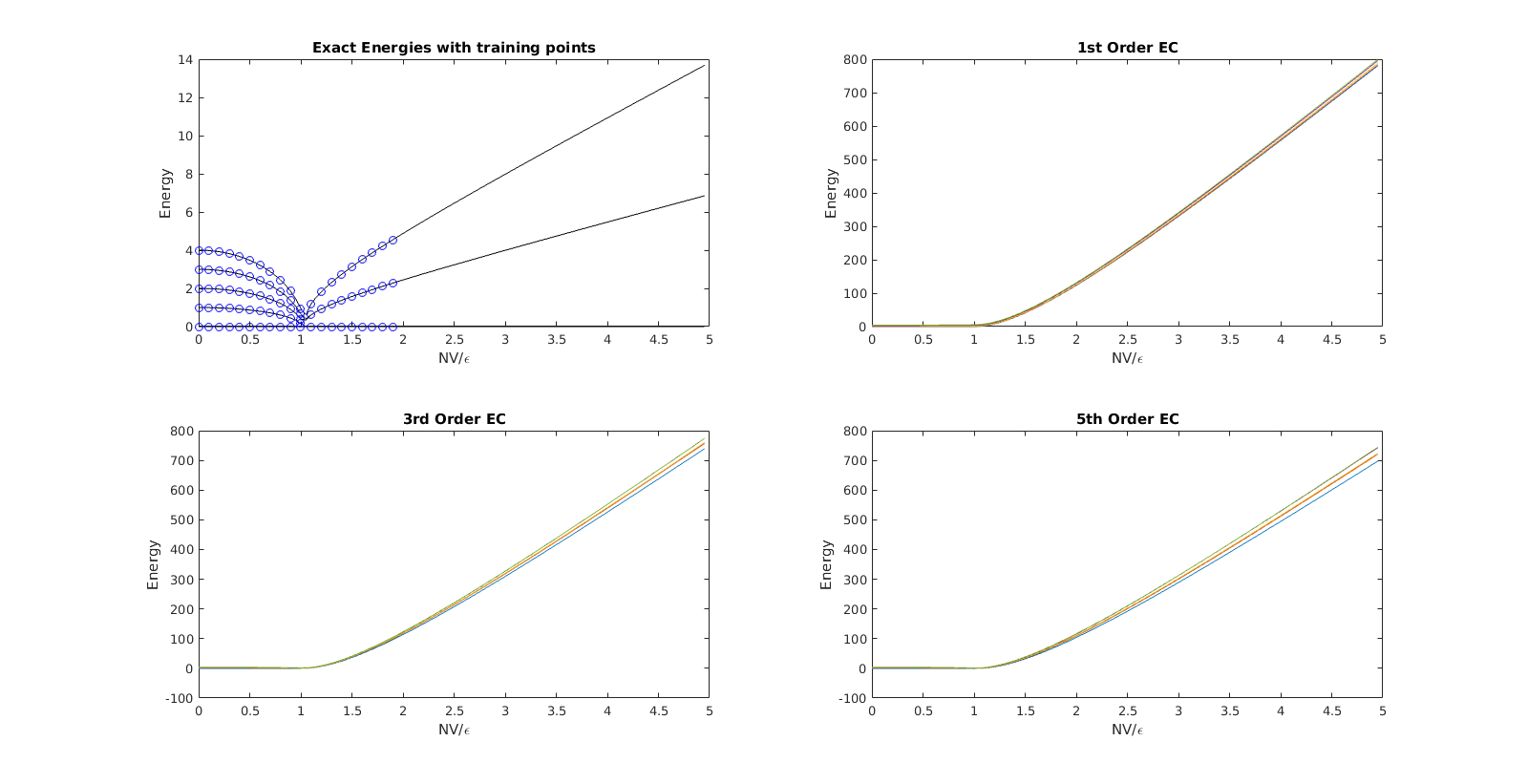
Figure 4.30: EC estimates for the lowest 5 eigenvalues of the N=1000 Lipkin model. We show the energy with the lowest ground state eigenvalue subtracted out, to show the kink present in the spectrum. The EC results diverge rapidly past the branch point at $C=1$.

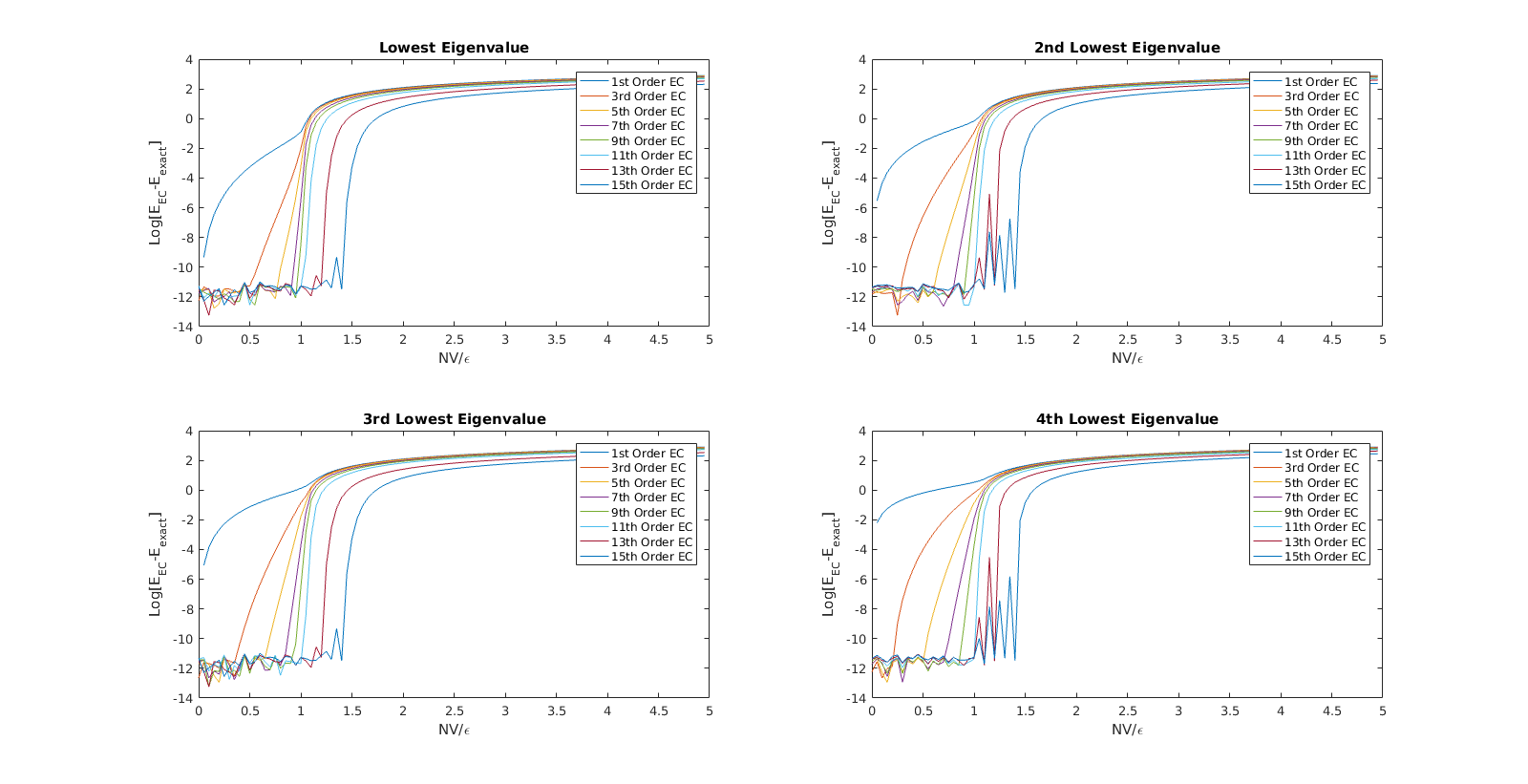
Figure 4.31: EC estimates for the lowest 5 eigenvalues of the N=1000 Lipkin model. We show the energy with the lowest ground state eigenvalue subtracted out, to show the kink present in the spectrum. The EC results diverge rapidly past the branch point at $C=1$.

Figure 4.32: Residuals for the first 4 eigenvalues for the N=1000 Lipkin model. The first 15 EC orders are shown for each eigenvalue.

We note that the EC method is not able to extrapolate past this kink in the spectrum. While the order-by-order estimates for the eigenvalues before that point get better and better, they all go bad by the time they reach the branch point.

Turning on the W term, we can move the location of the kink to around $C=3$. Like before, we consider up to 15th order EC, showing the results of the first five energy levels for odd EC orders in Figs. [4.33] and [4.34], with the corresponding residuals in Figs. [4.35].

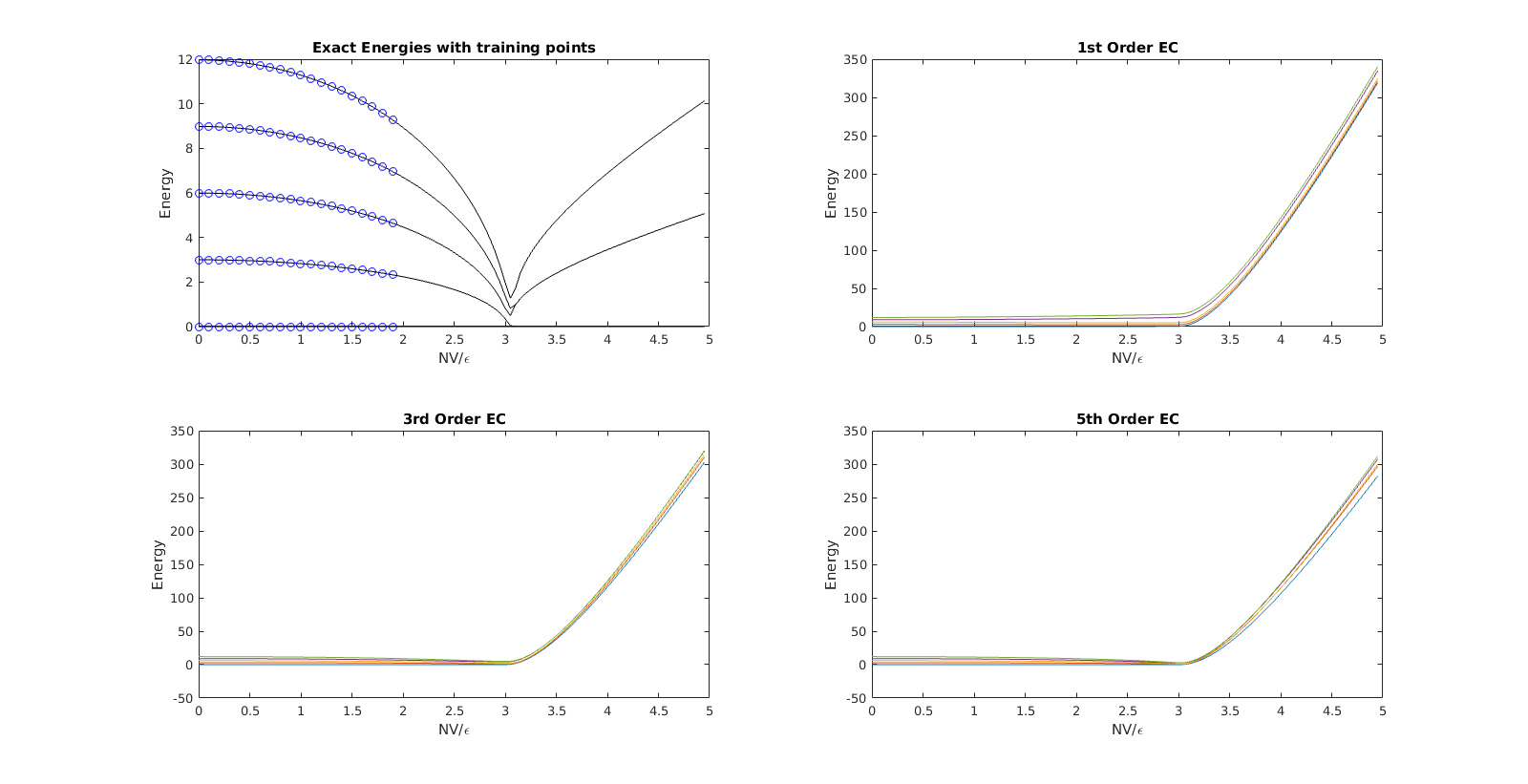
Figure 4.33: EC estimates for the lowest 5 eigenvalues of the N=1000 Lipkin model, with non-zero W. We show the energy with the lowest ground state eigenvalue subtracted out, to show the kink present in the spectrum. The EC results diverge rapidly past the branch point at $C=3$.

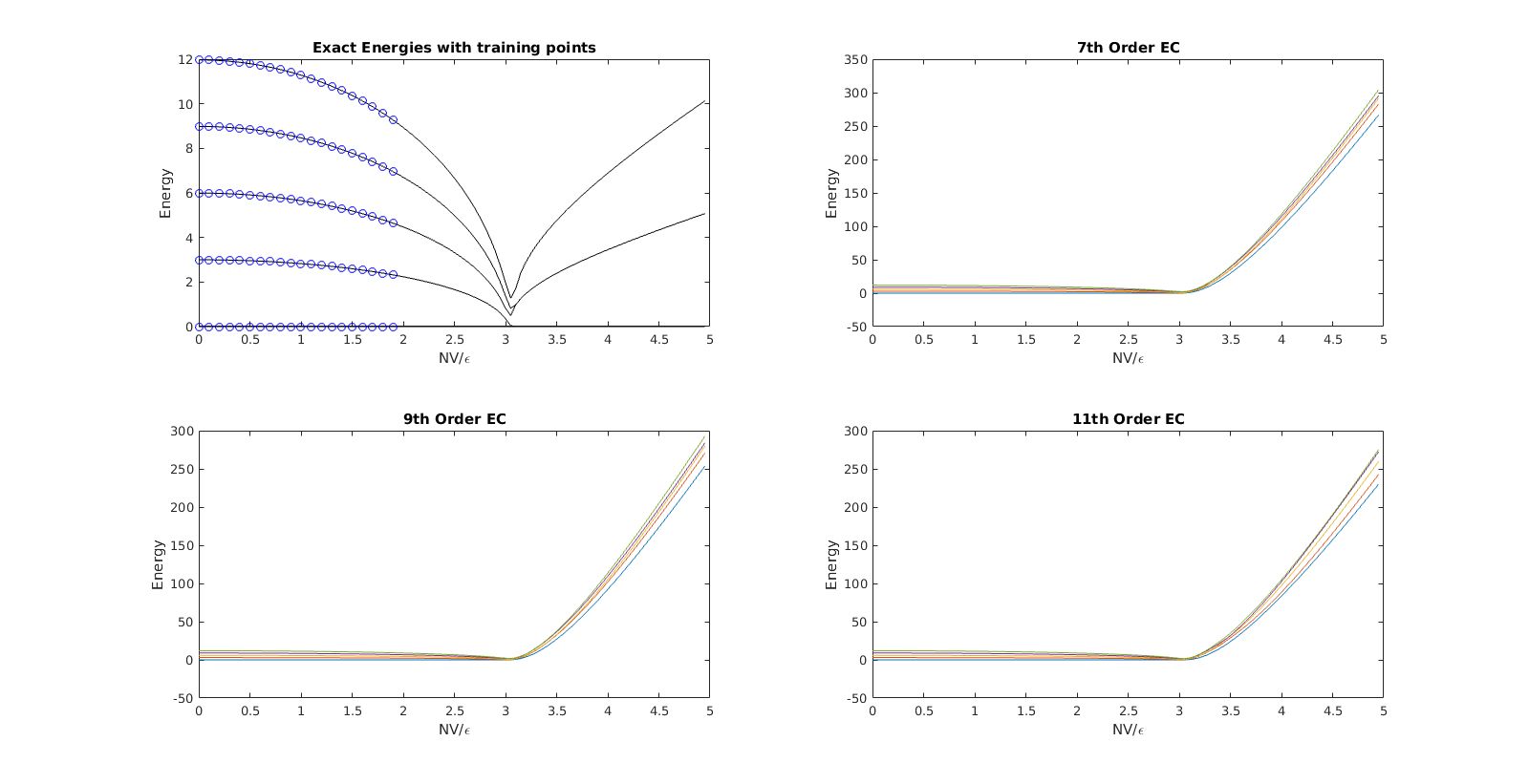
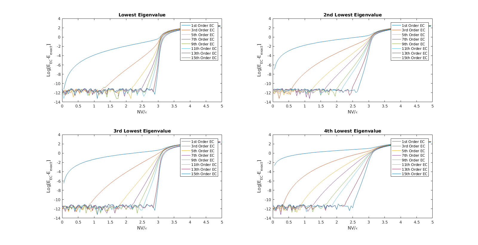
Figure 4.34: EC estimates for the lowest 5 eigenvalues of the N=1000 Lipkin model, with non-zero W. We show the energy with the lowest ground state eigenvalue subtracted out, to show the kink present in the spectrum. The EC results diverge rapidly past the branch point at $C=3$.

Figure 4.35: Residuals for the first 4 eigenvalues for the N=1000 Lipkin model, with non-zero W. The first 15 EC orders are shown for each eigenvalue.

Chapter 5 Concluding Remarks

In this work, we have demonstrated a new technique for evaluating the extremal eigenvalues and eigenvectors at points inaccessible to direct calculations. This technique relies on forming a low-dimensional space out of the eigenvectors in some coupling region, and then projecting the Hamiltonian at some target coupling into this space. Using analytic function theory, we showed that this projected Hamiltonian can be used to determine the analytically continued eigenvalues and eigenvectors at the target coupling.

As an application of this method, we considered four lattice systems. First, we considered the Bose-Hubbard model, which consists of $N$ bosons on a lattice, with a Hamiltonian consisting of a hopping term, and pair-wise interaction, and a chemical potential. This system has a phase transition which cannot be captured easily in perturbation theory, when the system goes from a weakly bound Bose gas, to a strongly bound cluster state. Using eigenvector continuation, we showed that this phase transition could be captured. The second system studied was pure neutron matter, done at leading order in Chiral EFT for a system of six and fourteen neutrons. In direct calculations, the sign problem prevented accurate results from being obtained, but by the use of eigenvector continuation, we could obtain accurate, large projection time estimates for the energies. Next, we looked at the non-perturbative inclusion of the Coulomb interaction into our lattice calculations. Since the Coulomb interaction is repulsive, it has a sign problem for large systems. We showed once again that the direct calculations yielded poor results, and that the use of the eigenvector continuation technique could dramatically help the determinations of the energy. Finally, we looked at the Lipkin model, which consists of N fermions distributed into two N-fold degenerate angular momentum levels. This levels are coupled, and allowed to mix, giving interesting phase transitions. Like in the Bose-Hubbard model, we showed that perturbation theory failed to capture this phase transition, and that the eigenvector continuation method did a good job at reproducing the energy levels.

In the future, we have two primary avenues to continue this work. One is on the mathematical side, looking at proving the convergence of this method, or providing error bounds on the estimates of the eigenvalues. The other direction this work could continue is in the applications to other systems; ones with more impact, like in QCD or in scattering calculations. The eigenvector continuation technique is very basic, so the number of research areas where it could be applied are quite broad. We would like to continue the search for applications, as we continue the work on the mathematical foundations of the method.

References

- [1] Gert Aarts and Ion-Olimpiu Stamatescu. Stochastic quantization at finite chemical potential. JHEP, 09:018, 2008.
- [2] Andrei Alexandru, Paulo F. Bedaque, Henry Lamm, and Scott Lawrence. Finite-Density Monte Carlo Calculations on Sign-Optimized Manifolds. Phys. Rev., D97(9):094510, 2018.
- [3] Andrei Alexandru, Manfried Faber, Ivan Horvath, and Keh-Fei Liu. Lattice QCD at finite density via a new canonical approach. Phys. Rev., D72:114513, 2005.
- [4] Y. Alhassid, D. J. Dean, S. E. Koonin, G. Lang, and W. E. Ormand. Practical solution to the monte carlo sign problem: Realistic calculations of . Phys. Rev. Lett., 72:613–616, Jan 1994.
- [5] J. M. Arias and J. E. García-Ramos. Scaling Properties of the Lipkin Model at the Critical Point. In Symmetries and Order: Algebraic Methods in Many Body Systems: In honor of Francesco Iachello, on the occasion of his retirement New Haven, CT, October 5-6, 2018, 2019.
- [6] G. F. Bertsch, D. J. Dean, and W. Nazarewicz. Computing atomic nuclei. SciDAC Review, 6:42, 2007.
- [7] D. Bindel, J. Demmel, and M. J. Friedman. Continuation of invariant subspaces in large bifurcation problems. SIAM J. Scientific Computing, 30:637–656, 01 2008.
- [8] D. Bindel, M. Friedman, W. Govaerts, J. Hughes, and Yu.A. Kuznetsov. Numerical computation of bifurcations in large equilibrium systems in matlab. Journal of Computational and Applied Mathematics, 261:232 – 248, 2014.
- [9] Shailesh Chandrasekharan. Fermion Bag Approach to Fermion Sign Problems. Eur. Phys. J., A49:90, 2013.
- [10] Giampaolo Co’ and Stefano De Leo. Analytical and numerical analysis of the complete Lipkin–Meshkov–Glick Hamiltonian. Int. J. Mod. Phys., E27(05):1850039, 2018.
- [11] J. Cox, C. Gattringer, K. Holland, B. Scarlet, and U.-J. Wiese. Meron-cluster solution of fermion and other sign problems. Nuclear Physics B - Proceedings Supplements, 83-84:777 – 791, 2000. Proceedings of the XVIIth International Symposium on Lattice Field Theory.
- [12] M. Cristoforetti, F. Di Renzo, A. Mukherjee, and L. Scorzato. Quantum field theories on the Lefschetz thimble. PoS, LATTICE2013:197, 2014.
- [13] Marco Cristoforetti, Francesco Di Renzo, and Luigi Scorzato. New approach to the sign problem in quantum field theories: High density QCD on a Lefschetz thimble. Phys. Rev., D86:074506, 2012.
- [14] Philippe de Forcrand and Slavo Kratochvila. Finite density QCD with a canonical approach. Nucl. Phys. Proc. Suppl., 153:62–67, 2006. [,62(2006)].
- [15] Philippe de Forcrand and Owe Philipsen. The Chiral critical line of N(f) = 2+1 QCD at zero and non-zero baryon density. JHEP, 01:077, 2007.
- [16] H. A. Dijkstra, F. W. Wubs, A. K. Cliffe, E. Doedel, I. F. Dragomirescu, B. Eckhardt, A. Yu. Gelfgat, A. L. Hazel, V. Lucarini, A. G. Salinger, and et al. Numerical bifurcation methods and their application to fluid dynamics: Analysis beyond simulation. Communications in Computational Physics, 15(1):1–45, 2014.
- [17] Simon Duane, A.D. Kennedy, Brian J. Pendleton, and Duncan Roweth. Hybrid monte carlo. Physics Letters B, 195(2):216 – 222, 1987.
- [18] S. Elhatisari, E. Epelbaum, H. Krebs, T. A. Lähde, D. Lee, N. Li, B.-N. Lu, U.-G. Meißner, and G. Rupak. Ab initio calculations of the isotopic dependence of nuclear clustering. Phys. Rev. Lett., 119:222505, Dec 2017.
- [19] S. Elhatisari, D. Lee, U.-G. Meißner, and G. Rupak. Nucleon-deuteron scattering using the adiabatic projection method. The European Physical Journal A, 52(6):174, 2016.
- [20] S. Elhatisari, D. Lee, G. Rupak, E. Epelbaum, H. Krebs, T. A. Lähde, T. Luu, and U.-G. Meißner. Ab-initio alpha-alpha scattering. Nature, 528:111–114, 2015.
- [21] S. Elhatisari, N. Li, A. Rokash, J. M. Alarcón, D. Du, N. Klein, B.-N. Lu, U.-G. Meißner, E. Epelbaum, H. Krebs, T. A. Lähde, D. Lee, and G. Rupak. Nuclear binding near a quantum phase transition. Phys. Rev. Lett., 117:132501, Sep 2016.
- [22] Evgeny Epelbaum, Hermann Krebs, Dean Lee, and Ulf-G. Meissner. Ground state energy of dilute neutron matter at next-to-leading order in lattice chiral effective field theory. Eur. Phys. J., A40:199–213, 2009.
- [23] Evgeny Epelbaum, Hermann Krebs, Dean Lee, and Ulf-G. Meissner. Lattice chiral effective field theory with three-body interactions at next-to-next-to-leading order. Eur. Phys. J., A41:125–139, 2009.
- [24] Evgeny Epelbaum, Hermann Krebs, Timo A. Lähde, Dean Lee, and Ulf-G. Meißner. Dependence of the triple-alpha process on the fundamental constants of nature. Eur. Phys. J., A49:82, 2013.
- [25] Evgeny Epelbaum, Hermann Krebs, Timo A. Lähde, Dean Lee, Ulf-G. Meißner, and Gautam Rupak. Ab Initio Calculation of the Spectrum and Structure of 16O. Phys. Rev. Lett., 112(10):102501, 2014.
- [26] M. Tanabashi et al. (Particle Data Group). Review of particle physics. Phys. Rev. D, 98, 2018.
- [27] Z. Fodor and S. D. Katz. A New method to study lattice QCD at finite temperature and chemical potential. Phys. Lett., B534:87–92, 2002.
- [28] D. Frame, I. He, R.and Ipsen, Da. Lee, De. Lee, and E. Rrapaj. Eigenvector continuation with subspace learning. Phys. Rev. Lett., 121(3):032501, 2018.
- [29] F. Fucito, E. Marinari, G. Parisi, and C. Rebbi. A Proposal for Monte Carlo Simulations of Fermionic Systems. Nucl. Phys., B180:369, 1981. [,586(1980)].
- [30] H. A. Gersch and G. C. Knollman. Quantum cell model for bosons. Phys. Rev., 129:959–967, Jan 1963.
- [31] S. Giorgini, L. P. Pitaevskii, and S. Stringari. Theory of ultracold atomic fermi gases. Rev. Mod. Phys., 80:1215–1274, Oct 2008.
- [32] D. J. Griffiths. Introduction to Quantum Mechanics. Cambridge University Press, 2016.
- [33] M. Hjorth-Jensen and collaborators. An advanced course in computational nuclear physics. Lect. Notes Phys., 936, 2017.
- [34] Yi Huang, Tongcang Li, and Zhang-qi Yin. Symmetry-breaking dynamics of the finite-size Lipkin-Meshkov-Glick model near ground state. Phys. Rev. A, 97(1):012115, Jan 2018.
- [35] J. Hubbard. Calculation of partition functions. Phys. Rev. Lett., 3:77–78, Jul 1959.
- [36] F. Iachello. Analytic description of critical point nuclei in a spherical-axially deformed shape phase transition. Phys. Rev. Lett., 87:052502, Jul 2001.
- [37] Ilse C. F. Ipsen and Dean J. Lee. Determinant Approximations. arXiv e-prints, page arXiv:1105.0437, May 2011.
- [38] N. Ishii, S. Aoki, and T. Hatsuda. The Nuclear Force from Lattice QCD. Phys. Rev. Lett., 99:022001, 2007.
- [39] Nico Klein, Dean Lee, Weitao Liu, and Ulf-G. Meißner. Regularization Methods for Nuclear Lattice Effective Field Theory. Phys. Lett., B747:511–516, 2015.
- [40] Nico Klein, Dean Lee, and Ulf-G. Meißner. Lattice Improvement in Lattice Effective Field Theory. Eur. Phys. J., A54(12):233, 2018.
- [41] T. A. Lähde, T. Luu, D. Lee, U.-G. Meißner, E. Epelbaum, H. Krebs, and G. Rupak. Nuclear lattice simulations using symmetry-sign extrapolation. The European Physical Journal A, 51(7):92, Jul 2015.
- [42] C. Lanczos. An iteration method for the solution of the eigenvalue problem of linear differential and integral operators. Journal of Research of the National Bureau of Standards, 45, 10 1950.
- [43] Kurt Langfeld and Biagio Lucini. Form the density-of-states method to finite density quantum field theory. Acta Phys. Polon. Supp., 9:503–514, 2016.
- [44] D. Lee. Ground state energy at unitarity. Phys. Rev. C, 78:024001, Aug 2008.
- [45] D. Lee. Lattice simulations for few- and many-body systems. Progress in Particle and Nuclear Physics, 63(1):117 – 154, 2009.
- [46] D. Lee. From Nuclear Forces and Effective Field Theory to Nuclear Structure and Reactions. Acta Phys. Polon., B50(3):253, 2019.
- [47] D. Lee, N. Salwen, and M. Windoloski. Introduction to stochastic error correction methods. Physics Letters B, 502(1):329 – 337, 2001.
- [48] N. Li, S. Elhatsari, E. Epelbaum, D. Lee, B.-N. Lu, and U.-G. Meissner. Neutron-proton scattering with lattice chiral effective field theory at next-to-next-to-next-to-leading order. Phys. Rev. C, 98:1–75, Oct 2018.
- [49] Ning Li, Serdar Elhatisari, Evgeny Epelbaum, Dean Lee, Bing-Nan Lu, and Ulf-G. Meißner. Galilean invariance restoration on the lattice. 2019.
- [50] H. Lipkin, N. Meshkov, and A. Glick. Validity of many-body approximation methods for a solvable model. Nuclear Physics, 1965.
- [51] B.-N. Lu, N. Li, S. Elhatsari, E. Epelbaum, D. Lee, , and U.-G. Meissner. Essential elements for nuclear binding.
- [52] Bing-Nan Lu, Timo A. Lähde, Dean Lee, and Ulf-G. Meißner. Precise determination of lattice phase shifts and mixing angles. Phys. Lett., B760:309–313, 2016.
- [53] Timo A. Lähde, Evgeny Epelbaum, Hermann Krebs, Dean Lee, Ulf-G. Meißner, and Gautam Rupak. Lattice effective field theory for nuclei from A = 4 to A = 28. 2013. [PoSLATTICE2013,231(2014)].
- [54] Timo A. Lähde, Evgeny Epelbaum, Hermann Krebs, Dean Lee, Ulf-G. Meißner, and Gautam Rupak. The Hoyle state in nuclear lattice effective field theory. Pramana, 83(5):651–659, 2014.
- [55] Timo A. Lähde, Evgeny Epelbaum, Hermann Krebs, Dean Lee, Ulf-G. Meißner, and Gautam Rupak. Uncertainties of Euclidean Time Extrapolation in Lattice Effective Field Theory. J. Phys., G42(3):034012, 2015.
- [56] R. Machleidt and D. R. Entem. Chiral effective field theory and nuclear forces. Phys. Rep., 503:1–75, 2011.
- [57] Nicholas Metropolis, Arianna W. Rosenbluth, Marshall N. Rosenbluth, Augusta H. Teller, and Edward Teller. Equation of state calculations by fast computing machines. The Journal of Chemical Physics, 21(6):1087–1092, 1953.
- [58] P.J.E. Peebles. Quantum Mechanics. Princeton University Press, 1992.
- [59] M. E. Peskin and D. V. Schroeder. An Introduction to Quantum Field Theory. Avalon Publishing, 2002.
- [60] Press, Flannery, Teukolsky, and Vetterling. Numerical Recipes in C. Cambridge University Press, 1988.
- [61] H. J. Rothe. Lattice Gauge Theories: An Introduction 4th Edition. World Scientific Publishing Company, 2012.
- [62] Y. Saad. Numerical methods for large eigenvalue problems. Classics in Applied Mathematics, 66, 2011.
- [63] Y. Saad. Analysis of subspace iteration for eigenvalue problems with evolving matrices. SIAM Journal on Matrix Analysis and Applications, 37:103–122, 01 2016.
- [64] J.J. Sakurai and J. Napolitano. Modern Quantum Mechanics 2nd Edition. Addison-Wesley, 2011.
- [65] Stephan Scherer. Introduction to chiral perturbation theory. Adv. Nucl. Phys, 27, 2003.
- [66] P. Sirkovic and D. Kressner. Subspace acceleration for large-scale parameter-dependent hermitian eigenproblems. SIAM Journal on Matrix Analysis and Applications, 37, 04 2015.
- [67] Pavel Stránský, Martin Dvořák, and Pavel Cejnar. Exceptional points near first- and second-order quantum phase transitions. Phys. Rev. E, 97(1):012112, Jan 2018.
- [68] P.A. Tipler and R.A. Llewellyn. Modern Physics. W.H. Freeman and Company, 2002.
- [69] Qian Wang and Francisco Perez-Bernal. Excited-state quantum phase transition and the quantum speed limit. arXiv e-prints, page arXiv:1810.03517, Oct 2018.
- [70] B. P. Welford. Note on a method for calculating corrected sums of squares and products. Technometrics, 1926.
- [71] K. G. Wilson. Confinement of quarks. Phys. Rev. D, 10:2445–2459, Oct 1974.
- [72] Biao-Liang Ye, Bo Li, Xianqing Li-Jost, and Shao-Ming Fei. Quantum correlations in critical XXZ system and LMG model. International Journal of Quantum Information, 16(3):1850029, Jan 2018.