The Polarising Fragmentation Function and the
$\Lambda$ polarisation in $e^{+}e^{-}$ processes

Abstract

The surprising polarisation of $\Lambda$s and other hyperons measured in many unpolarised hadronic processes, $p\,N\to\Lambda^{\uparrow}\,X$, has been a long standing challenge for QCD phenomenology. One possible explanation was suggested, related to non perturbative properties of the quark hadronisation process, and encoded in the so-called Polarising Fragmentation Function (PFF). Recent Belle data have shown a non zero $\Lambda$ polarisation also in unpolarised $e^{+}e^{-}$ processes, $e^{+}e^{-}\to\Lambda\,X$ and $e^{+}e^{-}\to\Lambda\,h\,X$. We consider the single inclusive case and the role of the PFFs. Adopting a simplified kinematics it is shown how they can originate a polarisation $P_{\Lambda}\not=0$ and give explicit expressions for it in terms of the PFFs. Although the Belle data do not allow yet, in our approach, an extraction of the PFFs, some clear predictions are given, suggesting crucial measurements, and estimates of $P_{\Lambda}$ are computed, in qualitative agreement with the Belle data.

I Introduction

The polarisation of $\Lambda$ hyperons inclusively produced in the high energy interactions of unpolarised hadrons, $p\,N\to\Lambda^{\uparrow}\,X$ Bunce:1976yb ; Heller:1978ty , is a major challenge for QCD theoretical interpretations since many years. A large amount of data is available Heller:1996pg , due to the fact that the weak decay of the $\Lambda$ allows an easy measurement of its polarisation $P_{\Lambda}$. No definite explanation of the origin of $P_{\Lambda}$, in a QCD framework, is convincingly available. In the usual application of perturbative QCD and collinear factorisation, the elementary interactions among unpolarised partons cannot produce any significant final state quark polarisation Kane:1978nd .

Non perturbative QCD features have been invoked. In Ref. Anselmino:2000vs and in Ref. Anselmino:2001js Transverse Momentum Dependent (TMD) effects in the fragmentation process were introduced, adopting a TMD factorisation scheme, respectively in proton-proton ($p\,p$) and lepton-proton ($\ell\,p$) interactions. In Ref. Zhou:2008fb collinear higher-twist quark-gluon-antiquark correlations in the nucleon were considered for $\ell\,p$ and $p\,p$ processes, while in Refs. Koike:2017fxr and Gamberg:2018fwy a complete twist-3 collinear fragmentation contribution to polarised hyperon production in unpolarised hadronic and $e^{+}e^{-}$ collisions has been presented. The TMD effects in the quark fragmentation of Refs. Anselmino:2000vs ; Anselmino:2001js were encoded in the so called Polarising Fragmentation Function (PFF), introduced and defined in Ref. Mulders:1995dh .

Very recently new data on the polarisation of $\Lambda$ hyperons produced in unpolarised $e^{+}e^{-}$ annihilation processes, $e^{+}e^{-}\to\Lambda\,h\,X$ and $e^{+}e^{-}\to({\rm jet})\,\Lambda\,X$, have been published by the Belle Collaboration Guan:2018ckx , showing a non zero value of $P_{\Lambda}$. Prompted by these data and the simplicity of the process which only depends on fragmentation functions, we consider in this paper the role of the transverse momentum dependent PFF in generating the $\Lambda$ polarisation. A general theoretical discussion of two hadron inclusive production in $e^{+}e^{-}$ interactions can be found in Ref. Boer:1997mf .

Our aim is that of understanding the physical mechanism through which the particular correlation between the momentum of the fragmenting quark, the momentum of the final $\Lambda$ and its polarisation - described by the PFF - can build up the $\Lambda$ polarisation. To do so we will adopt a very simple kinematical configuration which allows analytical computations and a direct visualisation of the process. It allows to understand specific features of $P_{\Lambda}$, which are true beyond the approximate kinematics and provide genuine testable predictions. Although the actual data of the Belle Collaboration, as it will be explained in Section III, do not allow a precise direct comparison with our computation of $P_{\Lambda}$, our estimates result in good qualitative agreement with the data.

II Formalism and simple analytical results for $P_{\Lambda}$

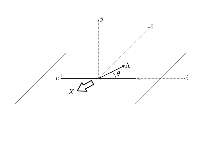
Figure 1: Definition of the c.m. reference frame for the process $e^{+}e^{-}\to\Lambda\,X$

We consider the process $e^{+}e^{-}\to\Lambda(\mbox{\boldmath$P$})\,X$ in the c.m. reference frame defined in Fig. 1, with:

$$\mbox{\boldmath$p$}_{e^{+}}\equiv\mbox{\boldmath$p$}=\frac{\sqrt{s}}{2}(0,\,0,\,1)\quad\quad\quad\mbox{\boldmath$p$}_{e^{-}}=-\mbox{\boldmath$p$}=\frac{\sqrt{s}}{2}(0,\,0,\,-1)\quad\quad\quad\mbox{\boldmath$p$}_{\Lambda}=p_{\Lambda}(\sin\theta,\,0,\,\cos\theta)\>,$$ (1)

where masses have been neglected. The initial leptons are unpolarised, while we consider the spin polarisation vector $P$ of the $\Lambda$ hyperon. Notice that, by parity invariance, the dependence of the cross section on $P$ must be of the form $\mbox{\boldmath$P$}\cdot\mbox{\boldmath$p$}\times\mbox{\boldmath$p$}_{\Lambda}\sim\sin\theta$ and $P$ can only be perpendicular to the production plane.

The $\Lambda$ production, at leading order, goes via the subprocess $e^{+}e^{-}\to q\,\bar{q}$, with the subsequent fragmentation of a quark into the $\Lambda$, such that

$$\mbox{\boldmath$p$}_{\Lambda}=z\,\mbox{\boldmath$p$}_{q}+\mbox{\boldmath$p$}_{\perp}\>$$ (2)

where

$$\mbox{\boldmath$p$}_{q}\cdot\mbox{\boldmath$p$}_{\perp}=0\quad\quad\quad p_{\Lambda}^{2}=\frac{z^{2}s}{4}+p_{\perp}^{2}\>.$$ (3)

The fragmentation function of an unpolarised quark into a spin 1/2 $\Lambda$ hyperon with polarisation vector along the $\uparrow=\mbox{\boldmath$P$}$ or $\downarrow=-\mbox{\boldmath$P$}$ directions can be written as

$$D_{\Lambda^{\uparrow,\downarrow}/q}(z,\mbox{\boldmath$p$}_{\perp})=\frac{1}{2}D_{\Lambda/q}(z,p_{\perp})\pm\frac{1}{2}\,\Delta^{N}D_{\Lambda^{\uparrow}/q}(z,p_{\perp})\,\mbox{\boldmath$P$}\cdot\hat{\mbox{\boldmath$p$}}_{q}\times\hat{\mbox{\boldmath$p$}}_{\perp}$$ (4)

where $D_{\Lambda/q}(z,p_{\perp})$ is the unpolarised Transverse Momentum Dependent Fragmentation Function (TMD-FF) and $\Delta^{N}D_{\Lambda^{\uparrow}/q}(z,p_{\perp})$ is the Polarising Fragmentation Function (PFF): it encodes basic features of the quark hadronisation process and describes the number density of spin 1/2 polarised hadrons ($\Lambda$ hyperons in this case) resulting from the fragmentation of an unpolarised quark. The angular dependence, $\mbox{\boldmath$P$}\cdot\hat{\mbox{\boldmath$p$}}_{q}\times\hat{\mbox{\boldmath$p$}}_{\perp}$, is dictated by parity invariance.

The cross section for the production of a $\Lambda$ hyperon with spin polarisation vector $\uparrow$ or $\downarrow$ in $e^{+}e^{-}$ annihilation, can be written, assuming TMD factorisation at leading order Boglione:2017jlh , as a convolution of the elementary annihilation cross section ($d\hat{\sigma}^{q}$) and the fragmentation function:

$$d\sigma^{\uparrow,\downarrow}=\sum_{q}e_{q}^{2}\>d\hat{\sigma}^{q}\otimes D_{\Lambda^{\uparrow,\downarrow}/q}\>,$$ (5)

where $q=u,\bar{u},d,\bar{d},s,\bar{s}$ quarks. The unpolarised cross section is given by

$$d\sigma^{\uparrow}+d\sigma^{\downarrow}=\sum_{q}e_{q}^{2}\>d\hat{\sigma}^{q}\otimes D_{\Lambda/q}\>,$$ (6)

the cross section difference by

$$d\sigma^{\uparrow}-d\sigma^{\downarrow}=\sum_{q}e_{q}^{2}\>d\hat{\sigma}^{q}\otimes\Delta^{N}D_{\Lambda^{\uparrow}/q}(z,p_{\perp})\,\mbox{\boldmath$P$}\cdot\hat{\mbox{\boldmath$p$}}_{q}\times\hat{\mbox{\boldmath$p$}}_{\perp}\>,$$ (7)

and the $\Lambda$ polarisation in the $P$ direction is given by

$$P_{\Lambda}=\frac{d\sigma^{\uparrow}-d\sigma^{\downarrow}}{d\sigma^{\uparrow}+d\sigma^{\downarrow}}\>\cdot$$ (8)

The convolutions in Eqs. (5)-(7) should take into account all possible momenta $\mbox{\boldmath$p$}_{q}$ of the fragmenting quark and all possible values of $\mbox{\boldmath$p$}_{\perp}$ such that $\mbox{\boldmath$p$}_{\Lambda}=z\,\mbox{\boldmath$p$}_{q}+\mbox{\boldmath$p$}_{\perp}$. Then, in general, the quark momentum $\mbox{\boldmath$p$}_{q}$ has also components outside the $xz$ $\Lambda$ production plane. However, the main contribution to a polarisation perpendicular to the $xz$ plane is originated, because of the cross product $\hat{\mbox{\boldmath$p$}}_{q}\times\hat{\mbox{\boldmath$p$}}_{\perp}$, by momenta in that plane. When computing the polarisation we then consider the simple kinematical configuration given in Fig. 2, in which, at fixed values of $z$ and $p_{\perp}$, there are two vectors $\mbox{\boldmath$p$}_{\perp}$ contributing to $\mbox{\boldmath$p$}_{\Lambda}$:

$$\mbox{\boldmath$p$}_{q_{1,2}}=\frac{\sqrt{s}}{2}(\sin\theta_{q_{1,2}},\,0,\,\cos\theta_{q_{1,2}})\quad\quad\quad\mbox{\boldmath$p$}_{\perp}^{(1,2)}=p_{\perp}(\pm\cos\theta_{q_{1,2}},\,0,\,\mp\sin\theta_{q_{1,2}})$$ (9)

where we have already imposed the condition $\mbox{\boldmath$p$}_{q}\cdot\mbox{\boldmath$p$}_{\perp}=0$.

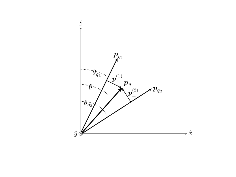
Figure 2: Simple 2-dimensional kinematical configuration. The $\hat{y}$-axis is entering the $xz$ plane.

We must also impose the condition (2):

$$p_{\Lambda}\sin\theta = z\frac{\sqrt{s}}{2}\sin\theta_{q_{1,2}}\pm p_{\perp}\cos\theta_{q_{1,2}}$$ (10)

$$p_{\Lambda}\cos\theta = z\frac{\sqrt{s}}{2}\cos\theta_{q_{1,2}}\mp p_{\perp}\sin\theta_{q_{1,2}}$$ (11)

with the solutions

$$\cos\theta_{q_{1,2}} = \frac{1}{\sqrt{1+\frac{\displaystyle 4p_{\perp}^{2}}{\displaystyle z^{2}s}}}\left(\cos\theta\pm\frac{2p_{\perp}}{z\sqrt{s}}\sin\theta\right)$$ (12)

$$\sin\theta_{q_{1,2}} = \frac{1}{\sqrt{1+\frac{\displaystyle 4p_{\perp}^{2}}{\displaystyle z^{2}s}}}\left(\sin\theta\mp\frac{2p_{\perp}}{z\sqrt{s}}\cos\theta\right)\cdot$$ (13)

As we said, the only polarisation allowed by parity invariance is orthogonal to the $xz$ production plane, that is $\mbox{\boldmath$P$}=\hat{}\mbox{\boldmath$y$}$. Notice that, in Eq. (7), according to our simple kinematical configuration of Fig. 2, we have:

$$\hat{\mbox{\boldmath$p$}}_{q_{1}}\times\hat{\mbox{\boldmath$p$}}_{\perp}^{(1)}=+\hat{}\mbox{\boldmath$y$}\quad\quad\quad\hat{\mbox{\boldmath$p$}}_{q_{2}}\times\hat{\mbox{\boldmath$p$}}_{\perp}^{(2)}=-\hat{}\mbox{\boldmath$y$}\>.$$ (14)

The convolution in Eq. (7) then reads:

$$\frac{d\sigma^{\uparrow}}{dz\,d(\cos\theta)}-\frac{d\sigma^{\downarrow}}{dz\,d(\cos\theta)}=\sum_{q}e_{q}^{2}\int\!p_{\perp}\,dp_{\perp}\left[\frac{d\hat{\sigma}^{q}}{d(\cos\theta_{q_{1}})}-\frac{d\hat{\sigma}^{q}}{d(\cos\theta_{q_{2}})}\right]\>\Delta^{N}D_{\Lambda^{\uparrow}/q}(z,p_{\perp})\>,$$ (15)

where the elementary $e^{+}e^{-}\to q\,\bar{q}$ cross section is given by

$$\frac{d\hat{\sigma}^{q}}{d\cos(\theta_{q})}=\frac{3\pi\alpha^{2}}{2s}(1+\cos^{2}\theta_{q})$$ (16)

and the expressions of $\cos\theta_{q_{1,2}}$ are given in Eq. (12).

By using Eqs. (16) and (12) in Eq. (15) one has a very simple result:

$$\frac{d\sigma^{\uparrow}}{dz\,d(\cos\theta)}-\frac{d\sigma^{\downarrow}}{dz\,d(\cos\theta)} = \frac{3\pi\alpha^{2}}{2s}\sum_{q}e_{q}^{2}\int\!p_{\perp}\,dp_{\perp}(\cos^{2}\theta_{q_{1}}-\cos^{2}\theta_{q_{2}})\>\Delta^{N}D_{\Lambda^{\uparrow}/q}(z,p_{\perp})$$ (17)

$$= \frac{3\pi\alpha^{2}}{2s}\sum_{q}e_{q}^{2}\int\!p_{\perp}\,dp_{\perp}\frac{4\,z\,p_{\perp}\sqrt{s}}{z^{2}s+4\,p_{\perp}^{2}}\>\sin(2\theta)\>\Delta^{N}D_{\Lambda^{\uparrow}/q}(z,p_{\perp})\>.$$ (18)

Some more comments on the physical interpretation of this expression and the approximations involved will be made in the next Section.

We have now to compute the unpolarised cross section, appearing in the denominator of Eq. (8). As, differently from the polarised case, now all components of $\mbox{\boldmath$p$}_{q}$ contribute equally to the $\Lambda$ production, and not only those in the $xz$ plane, we write the convolution (6) as:

$$\frac{d\sigma}{dz\,d(\cos\theta)} = \sum_{q}e_{q}^{2}\int\!2\pi\,p_{\perp}\,dp_{\perp}\frac{d\hat{\sigma}^{q}}{d(\cos\theta)}\>D_{\Lambda/q}(z,p_{\perp})$$ (19)

$$= \sum_{q}e_{q}^{2}\>\frac{d\hat{\sigma}^{q}}{d(\cos\theta)}\>D_{\Lambda/q}(z)$$ (20)

where, essentially, we have assumed $d\hat{\sigma}^{q}/d(\cos\theta_{q})\simeq d\hat{\sigma}^{q}/d(\cos\theta)$ and used the relation $\int d^{2}\mbox{\boldmath$p$}_{\perp}D_{\Lambda/q}(z,p_{\perp})=D_{\Lambda/q}(z)$. Eq. (20) is the usual expression for the cross section in the collinear partonic configuration.

By collecting Eqs. (8) and (16)–(20) we have simple expressions for the $\Lambda$ polarisation along the $\hat{}\mbox{\boldmath$y$}$ direction:

$$P_{\Lambda}(z,\cos\theta)=\frac{\displaystyle\sum_{q}e_{q}^{2}\int\!p_{\perp}\,dp_{\perp}\frac{4\,z\,p_{\perp}\sqrt{s}}{z^{2}s+4\,p_{\perp}^{2}}\>\Delta^{N}D_{\Lambda^{\uparrow}/q}(z,p_{\perp})}{\displaystyle\sum_{q}e_{q}^{2}\>D_{\Lambda/q}(z)}\>\frac{\sin(2\theta)}{1+\cos^{2}\theta}$$ (21)

$$P_{\Lambda}(z,p_{\perp})=\frac{\displaystyle\sum_{q}e_{q}^{2}\>\frac{4\,z\,p_{\perp}\sqrt{s}}{z^{2}s+4\,p_{\perp}^{2}}\>\Delta^{N}D_{\Lambda^{\uparrow}/q}(z,p_{\perp})}{\displaystyle\sum_{q}e_{q}^{2}\>2\pi\>D_{\Lambda/q}(z,p_{\perp})}\>\frac{\displaystyle\int\!d(\cos\theta)\>\sin(2\theta)}{\displaystyle\int\!d(\cos\theta)\>(1+\cos^{2}\theta)}$$ (22)

$$P_{\Lambda}(z,p_{\perp},\cos\theta)=\frac{\displaystyle\sum_{q}e_{q}^{2}\>\frac{4\,z\,p_{\perp}\sqrt{s}}{z^{2}s+4\,p_{\perp}^{2}}\>\Delta^{N}D_{\Lambda^{\uparrow}/q}(z,p_{\perp})}{\displaystyle\sum_{q}e_{q}^{2}\>2\pi\>D_{\Lambda/q}(z,p_{\perp})}\>\frac{\sin(2\theta)}{1+\cos^{2}\theta}\>\cdot$$ (23)

In the single inclusive $\Lambda$ production process that we are considering, the only observables are $z$ and $\cos\theta$, while the values of $p_{\perp}$ are integrated. We have also given Eqs. (22) and (23) as they might allow some comparison with the data of Ref. Guan:2018ckx .

III Comments, suggested measurements and some predictions

Before trying to give some estimates of the polarisation a few comments are in order, which illustrate the meaning and validity of the results obtained in the previous Section.

• Our simple 2-dimensional kinematical configuration shows clearly the mechanism which, thanks to the $\mbox{\boldmath$P$}\cdot\mbox{\boldmath$p$}_{q}\times\mbox{\boldmath$p$}_{\perp}$ correlation of the PFF, builds up the $\Lambda$ polarisation. As illustrated in Fig. 2, at any fixed values of $z$ and $p_{\perp}=|\mbox{\boldmath$p$}_{\perp}|$ there are two possible vectors $\mbox{\boldmath$p$}_{q}$ leading to the same $\mbox{\boldmath$p$}_{\Lambda}$. These two vectors lead to opposite vectors $\mbox{\boldmath$p$}_{q}\times\mbox{\boldmath$p$}_{\perp}=\mbox{\boldmath$p$}_{q}\times\mbox{\boldmath$p$}_{\Lambda}$ and then to opposite values of the polarisation along the $\mbox{\boldmath$P$}=\hat{}\mbox{\boldmath$y$}$ direction. However, in the convolution of Eqs. (7) and (15), to each of them there corresponds a different value of the scattering angle $\theta$ and then of the elementary cross section (16). This leads to a clear physical interpretation of Eqs. (17) and (18).

• Notice also that the annihilation cross section is symmetric around $\theta=\pi/2$, where $\cos^{2}\theta_{q_{1}}=\cos^{2}\theta_{q_{2}}$, Eq. (12); thus, the polarisation vanishes at $\theta=\pi/2$, reflecting the nature of the $e^{+}e^{-}\to q\,\bar{q}$ partonic interaction at leading order. In addition, as we already remarked, the polarisation must vanish at $\theta=0$ and $\theta=\pi$ for parity invariance: then one understands the $\sin(2\theta)$ behaviour of $P_{\Lambda}$.

• The true kinematical implementation of our mechanism should take into account a 3-dimensional configuration of $\mbox{\boldmath$p$}_{q}$ around $\mbox{\boldmath$p$}_{\Lambda}$. Then, always at fixed values of $z$ and $p_{\perp}$, we would have contributions from other pairs of vectors $\mbox{\boldmath$p$}_{q_{1}}$ and $\mbox{\boldmath$p$}_{q_{2}}$ out of the $xz$ plane. Such vectors contribute (oppositely) to $P_{\Lambda}$ only with their components in the $xz$ plane, which is smaller than $p_{\perp}$. In addition, for them the difference between $\theta_{q_{1}}$ and $\theta_{q_{2}}$ is also smaller. We estimate that their total contribution to $P_{\Lambda}$ would not change the value obtained in our limited 2-dimensional kinematical model by more than a factor 2. Our numerical computations will actually underestimate the value of the polarisation.

• The conclusions of the first two paragraphs of this Section are valid also in full 3-dimensional kinematics; the first one simply illustrates the PFF mechanism, while the second one is based on the symmetry properties, at leading order, of the elementary cross section, proportional to $(1+\cos^{2}\theta)$. Then, our result

  $$P_{\Lambda}\sim\sin(2\theta)$$ (24)

  is a genuine prediction of the way in which a PFF would build up the $\Lambda$ polarisation; a prediction which could and should be easily tested experimentally.

• We have given explicit expressions of $P_{\Lambda}(z,p_{\perp},\cos\theta)$, and some of their integrated forms, in terms of the unknown polarising fragmentation function $\Delta^{N}D_{\Lambda^{\uparrow}/q}(z,p_{\perp})$. The $\theta$ dependence, as we stressed in the previous paragraph, is instead well defined. Notice that we also find

  $$P_{\Lambda}={\cal O}(p_{\perp}/\sqrt{s}),$$ (25)

  meaning that the polarisation in the single inclusive process $e^{+}e^{-}\to\Lambda\,X$ is a higher twist effect. It agrees with the observation of a vanishing $\Lambda$ transverse polarisation in $e^{+}e^{-}$ at the $Z^{0}$ pole by the OPAL Collaboration Ackerstaff:1997nh .

In the single inclusive process that we are considering, one only observes the final $\Lambda$ and its polarisation, given by Eq. (21). Such a process allows to exploit the fact that one knows the direction of $\mbox{\boldmath$P$}_{\Lambda}$, perpendicular to the production plane. In addition, we have assumed that also the elementary dynamics takes predominantly place in the same plane. While the $\cos\theta$ dependence of the polarisation is definitely fixed by the PFF mechanism, independently of the simplified kinematics, its magnitude, $P_{\Lambda}(z,\cos\theta)$, depends on our assumption and on the functional form of the PFF $\Delta^{N}D_{\Lambda^{\uparrow}/q}(z,p_{\perp})$. If abundant and precise data were available for $P_{\Lambda}$ in the $e^{+}e^{-}\to\Lambda\,X$ process, one could try to parametrise the PFF, and, performing a best fit of the experimental points, extract information on the PFF.

Unfortunately, the available experimental information is not exactly what we would like to have in order to perform such a procedure. In Ref. Guan:2018ckx the inclusive $\Lambda$ polarisation is measured along the direction ${\hat{}\mbox{\boldmath$T$}}\times{\hat{}\mbox{\boldmath$p$}_{\Lambda}}$, where ${\hat{}\mbox{\boldmath$T$}}$ is the thrust axis, which, apart from unavoidable experimental inaccuracies, coincides with ${\hat{}\mbox{\boldmath$p$}}_{q}$. What actually the Belle Collaboration measure is the polarisation in the process $e^{+}e^{-}\to{\rm jet}\,\Lambda\,X$, which, in general, needs not be perpendicular to the $\Lambda$ production plane. Their polarisation is presented as a function of $p_{\perp}$ and $z$. Presumably, data have been collected over a wide range of the angle $\theta$, although this information cannot be found in the paper.

However, we can attempt a very qualitative comparison with the Belle data, by exploiting Eq. (23), which also gives, with some approximations, the polarisation along $\mbox{\boldmath$p$}_{q}\times\mbox{\boldmath$p$}_{\Lambda}$ as a function of $p_{\perp}$, $z$ and $\cos\theta$. Similarly, if we knew the range of $\theta$ covered by the experiment, we could use Eq. (22).

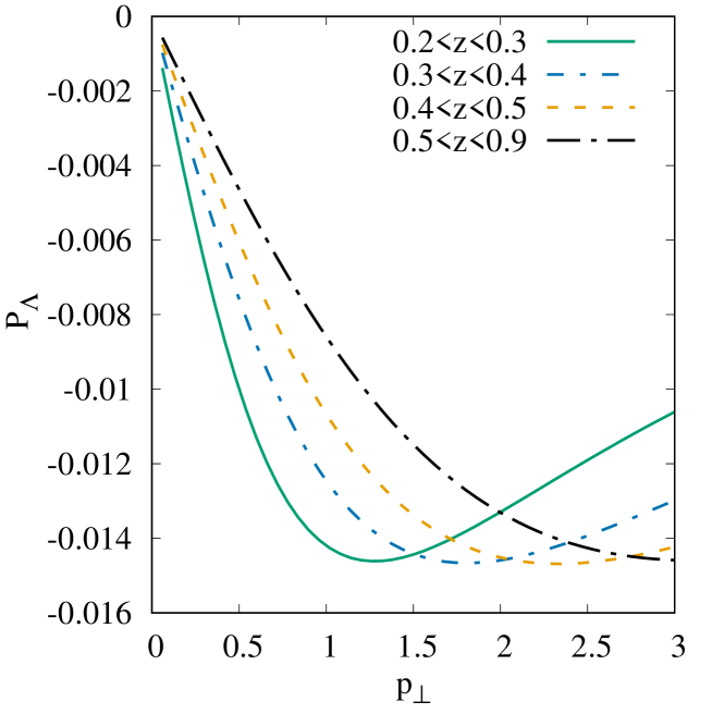
Figure 3: Plots of $P_{\Lambda}(p_{\perp},\theta=\pi/3))$ vs. $p_{\perp}$, computed according to Eq. (23). For each bin of $z$ values the numerator and denominator of Eq. (23) have been accordingly integrated. The PFFs are given in Eq. (26) and the FFs $D_{\Lambda/q}(z)$ are from Ref. deFlorian:1997zj .

Figure 4: Plots of $P_{\Lambda}(z,\theta=\pi/3))$ vs. $z$, computed according to Eq. (21), for different values of $\langle p^{2}_{\perp}\rangle$. We have integrated numerator and denominator of Eq. (21) in the range $0\leq p_{\perp}\leq 3$ GeV.

In order to obtain simple numerical estimates of $P_{\Lambda}$ we assume the PFFs, $\Delta^{N}D_{\Lambda^{\uparrow}/q}(z,p_{\perp})$, to be $20\%$ of the corresponding unpolarised TMD-FFs, $D_{\Lambda/q}(z,p_{\perp})$. In Ref. Anselmino:2001js the PFFs have been parameterised in terms of the unpolarised FFs and have been used to compute the $\Lambda$ polarisation in $p\,p\to\Lambda\,X$ processes. From the best fit parameters it is found that the overall normalisation factor for the $u$ and $d$ quark PFFs has to be negative whereas for $s$ quarks it has to be positive. Motivated by this, we choose

$$\Delta^{N}D_{\Lambda^{\uparrow}/u}(z,p_{\perp})=-0.2\times D_{\Lambda/u}(z,p_{\perp})$$

$$\Delta^{N}D_{\Lambda^{\uparrow}/d}(z,p_{\perp})=-0.2\times D_{\Lambda/d}(z,p_{\perp})$$ (26)

$$\Delta^{N}D_{\Lambda^{\uparrow}/s}(z,p_{\perp})=0.2\times D_{\Lambda/s}(z,p_{\perp})\>.$$

As usual, for the unpolarised TMD-FFs, we consider factorised $z$ and $p_{\perp}$ dependences, with a Gaussian parameterisation for the transverse momentum dependent part:

$$D_{\Lambda/q}(z,p_{\perp})=D_{\Lambda/q}(z)\>\frac{1}{\pi\,\langle p^{2}_{\perp}\rangle}\>e^{\displaystyle-\frac{p^{2}_{\perp}}{\langle p^{2}_{\perp}\rangle}}\>,$$ (27)

where $q=u,d,s$ and $D_{\Lambda/q}(z)$ is the collinear FF. The width of the Gaussian, $\langle p^{2}_{\perp}\rangle$, is a free parameter which could be extracted by fitting data from experiments.

In order to further simplify our order of magnitude estimates, we consider the LO collinear FF from Ref. deFlorian:1997zj , where it has been assumed, following simple $SU_{f}(3)$ symmetry arguments, that all the light flavour quarks fragment to $\Lambda$ with equal probability, i.e.,

$${}D_{\Lambda/u}=D_{\Lambda/d}=D_{\Lambda/s}\equiv D_{\Lambda/q}\>,$$ (28)

while the antiquark fragmentation into a $\Lambda$ are taken to be negligible, $D_{\Lambda/\bar{q}}=0$.

In the plots given in Fig. 3 we show $P_{\Lambda}$ as a function of $p_{\perp}$, computed according to Eq. (23), for different bins of $z$, similar to those of the Belle data Guan:2018ckx , and fixing $\theta=\pi/3$. For each plot we have integrated the numerator and denominator of Eq. (23) over $z$ according to the corresponding bin range. The LO collinear FFs $D_{\Lambda/q}(z)$ for light quarks have been taken from Ref. deFlorian:1997zj . Notice that, in this case, as a consequence of Eqs. (27) and (26), the flavour independent Gaussian widths $\langle p^{2}_{\perp}\rangle$ do not affect the value of $P_{\Lambda}(p_{\perp},\theta)$.

As we commented before, the actual comparison between our computation of $P_{\Lambda}$ and the Belle data can only be considered at a qualitative level. Our definition of $z$, Eq. (2), differs from the value of $z_{\Lambda}=2E_{\Lambda}/\sqrt{s}$, used in Ref. Guan:2018ckx , by terms of the order $p_{\perp}^{2}/(sz^{2})$. Moreover, our estimates of $P_{\Lambda}$ undervalue it. The signs of the PFFs have been assumed to be the same as those obtained in fitting the $\Lambda$ polarisation in $p\,p\to\Lambda\,X$ processes Anselmino:2001js . Despite all this, when comparing with Fig. 1 of Ref. Guan:2018ckx , the qualitative agreement is remarkable, with negative values of $P_{\Lambda}(p_{\perp})$ of the order of a few percents or less. Notice, however, that the sign of $P_{\Lambda}$ depends on the value of the production angle $\theta$ and changes at $\theta=\pi/2$.

In Fig. 4 we plot $P_{\Lambda}$ as a function of $z$ according to Eq. (21), for different values of $\langle p_{\perp}^{2}\rangle$, fixing $\theta=\pi/3$ and integrating numerator and denominator over $p_{\perp}$ between 0 and 3 GeV. Increasing the upper integration limit has negligible effects. Notice that, in this case, again as a consequence of Eqs. (27) and (26), the collinear FFs $D_{\Lambda/q}(z)$ cancel out in the ratio giving $P_{\Lambda}(z,\theta)$.

Again, with our choice of the PFFs, Eq. (26), we obtain, at the chosen $\theta$ angle, negative values of $P_{\Lambda}(z)$, of the order of 1%, in qualitative agreement with the Belle data Guan:2018ckx .

IV Conclusions

Motivated by new data on the polarisation of $\Lambda$ hyperons, measured by the Belle Collaboration in unpolarised $e^{+}e^{-}$ annihilation processes Guan:2018ckx , we have investigated the role of the Polarising Fragmentation Functions Anselmino:2000vs ; Anselmino:2001js ; Mulders:1995dh in generating the polarisation. These new data are particularly interesting as they refer to a process in which $P_{\Lambda}$ can only depend on the properties of the quark fragmentation, without the complication of convolutions with partonic distributions, such as in the case of $p\,N\to\Lambda^{\uparrow}\,X$ and $\ell\,N\to\Lambda^{\uparrow}\,X$ processes.

We have adopted a simplified 2-dimensional kinematics, which might lead to an underestimate of $P_{\Lambda}$, but has the merit of visualising the partonic process and the role of the PFFs. In addition, in our LO TMD factorisation scheme, we obtain a general clear prediction for the $\theta$ dependence of $P_{\Lambda}$, Eq. (24), which could be easily tested.

A precise comparison of the results of our approach with the few Belle data is not possible yet, because of the nature of the Belle data, which do not refer to a fully inclusive process, and to the uncertainty on the $\Lambda$ production angle $\theta$, not discussed in Ref. Guan:2018ckx . However, by making simple assumptions on the PFFs and the collinear FF, and following indications on the sign of the PFFs obtained by fitting the $\Lambda$ polarisation in $p\,p\to\Lambda^{\uparrow}\,X$ processes Anselmino:2000vs , we have given some estimates of the expected values of $P_{\Lambda}(p_{\perp})$ and $P_{\Lambda}(z)$ in the same $p_{\perp}$ and $z$ kinematical regions covered by the Belle measurements, fixing a particular value of $\theta$. Such estimates show a negative and small $\Lambda$ polarisation, in agreement with the Belle data.

- (1) G. Bunce et al., Phys. Rev. Lett. 36, 1113 (1976).
- (2) K. J. Heller et al., Phys. Rev. Lett. 41, 607 (1978); Erratum: [Phys. Rev. Lett. 45, 1043 (1980)].
- (3) For a review of the data, see, e.g.: K. J. Heller, in Proceedings of the 12th International Symposium on Spin Physics, Amsterdam, 1996 (World Scientific, Singapore, 1997).
- (4) G. L. Kane, J. Pumplin and W. Repko, Phys. Rev. Lett. 41, 1689 (1978).
- (5) M. Anselmino, D. Boer, U. D’Alesio and F. Murgia, Phys. Rev. D 63, 054029 (2001) [hep-ph/0008186].
- (6) M. Anselmino, D. Boer, U. D’Alesio and F. Murgia, Phys. Rev. D 65, 114014 (2002) [hep-ph/0109186].
- (7) J. Zhou, F. Yuan and Z. T. Liang, Phys. Rev. D 78, 114008 (2008) [arXiv:0808.3629 [hep-ph]].
- (8) Y. Koike, A. Metz, D. Pitonyak, K. Yabe and S. Yoshida, Phys. Rev. D 95, 114013 (2017) [arXiv:1703.09399 [hep-ph]].
- (9) L. Gamberg, Z. B. Kang, D. Pitonyak, M. Schlegel and S. Yoshida, JHEP 1901, 111 (2019) [arXiv:1810.08645 [hep-ph]].
- (10) P. J. Mulders and R. D. Tangerman, Nucl. Phys. B 461, 197 (1996); Erratum: [Nucl. Phys. B 484, 538 (1997)] [hep-ph/9510301].
- (11) Y. Guan et al. [Belle Collaboration], Phys. Rev. Lett. 122, 042001 (2019) [arXiv:1808.05000 [hep-ex]].
- (12) D. Boer, R. Jakob and P. J. Mulders, Nucl. Phys. B 504, 345 (1997) [hep-ph/9702281].
- (13) A discussion of the TMD factorisation in processes can be found in M. Boglione, J. O. Gonzalez-Hernandez and R. Taghavi, Phys. Lett. B 772, 78 (2017) [arXiv:1704.08882 [hep-ph]].
- (14) K. Ackerstaff et al. [OPAL Collaboration], Eur. Phys. J. C 2, 49 (1998) [hep-ex/9708027].
- (15) D. de Florian, M. Stratmann and W. Vogelsang, Phys. Rev. D 57, 5811 (1998) [hep-ph/9711387].