RACS: Rapid Analysis of ChIP-Seq data for contig based genomes
Abstract
Background: Chromatin immunoprecipitation coupled to next generation sequencing (ChIP-Seq) is a widely used technique to investigate the function of chromatin-related proteins in a genome-wide manner. ChIP-Seq generates large quantities of data which can be difficult to process and analyse, particularly for organisms with contig based genomes. Contig-based genomes often have poor annotations for cis-elements, for example enhancers, that are important for gene expression. Poorly annotated genomes make a comprehensive analysis of ChIP-Seq data difficult and as such standardized analysis pipelines are lacking.
Methods: We report a computational pipeline that utilizes traditional High-Performance Computing techniques and open source tools for processing and analysing data obtained from ChIP-Seq.
We applied our computational pipeline “Rapid Analysis of ChIP-Seq data” (RACS) to ChIP-Seq data that was generated in the model organism Tetrahymena thermophila, an example of an organism with a genome that is available in contigs.
Results: To test the performance and efficiency of RACs, we performed control ChIP-Seq experiments allowing us to rapidly eliminate false positives when analyzing our previously published data set. Our pipeline segregates the found read accumulations between genic and intergenic regions and is highly efficient for rapid downstream analyses.
Conclusions: Altogether, the computational pipeline presented in this report is an efficient and highly reliable tool to analyze genome-wide ChIP-Seq data generated in model organisms with contig-based genomes.
keywords:
Methodology article
[id=n1]Equal contributor
1 Background
In the last few years the traditional High Performance Computing (HPC) centres, such as SciNet at the University of Toronto [1], have been witnessing the emergence of increasing amounts of work-flows from non-typical disciplines in the field of computational science [2]. Among those, disciplines related to bioinformatics appear to be the most prominent in terms of demanding resources and tackling complex problems related to Next Generation Sequencing (NGS). The human genome project [3], the human microbiome project [4], RNA-Seq to analyze gene expression [5, 6] and ChIP-Seq to assess global DNA-binding sites [5, 6] are all examples of projects where HPC can be applied.
The advantage of NGS for researchers is high-throughput sequencing analysis allowing millions of DNA molecules to be read at the same time [7, 8, 9]. The output of NGS is substantial and it can be overwhelming for analyses [10, 11]. The difficulties during the analyses can be increased if the genome to be studied is more specific. We address this problem by combining and utilizing open-source tools such as BWA [12], SAMtools [13], Linux shell and R scripts [14] and techniques commonly employed in the HPC fields.
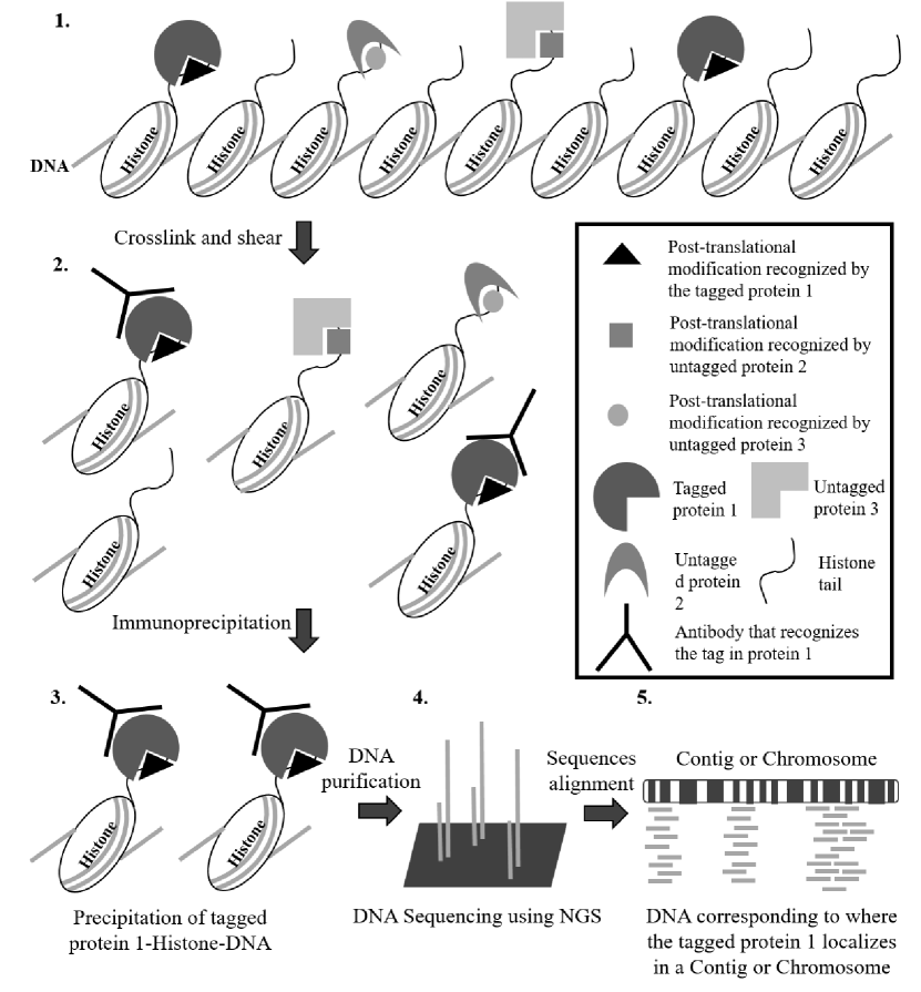
Chromatin immunoprecipitation coupled to NGS (ChIP-Seq, Figure 1) can be utilized to infer function(s) of a protein of interest based on its chromatin-occupancy profile. For instance, if the ChIP signal accumulates closer to a 5’ region of a gene, we could infer that protein’s function may be related to transcription initiation. On the other hand, accumulation of ChIP peaks at the 3’ ends would suggest a role in transcription termination. However, this has to be tested further since gene expression can also be coordinated by elements that are not in close proximity to the specific gene [15]. Utilization of mock/control samples (untagged) is important to account for nonspecific DNA interactions with the chromatography resin.
In multi-cellular eukaryotes, the mechanisms of chromatin remodeling involving the precise delineation of how transcription starts, progresses and ends are poorly understood. Chromatin remodeling research aids in our understanding of how these mechanisms affect cellular function in the progression of disease. ChIP-Seq is generally used as an initial step to examine the possible role(s) of a protein in chromatin re-modeling [9, 16].
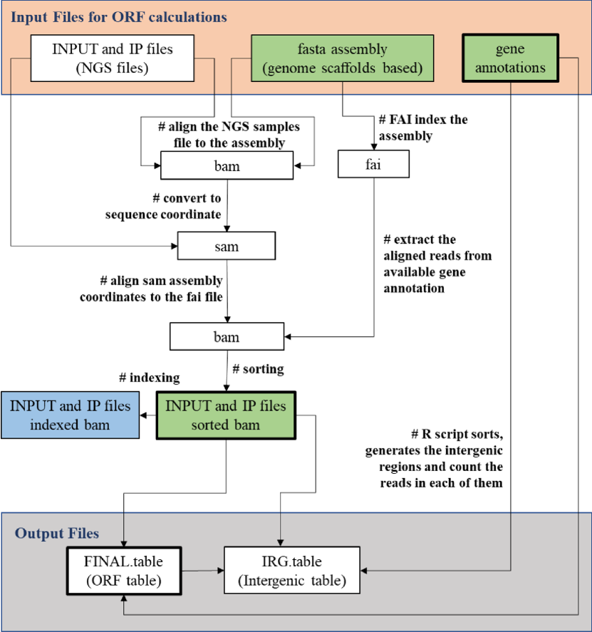
Many algorithms and visualization tools are already set for other model organisms such as human or yeast; however, none of these applications cater to contig based genomes with only minimal annotations of genes, as is the case in T.thermophila. These applications also do not directly address whether the accumulation of the protein of interest is in a genic or intergenic region. Using available tools, such as MACS2 [17], the user receives the peaks coordinates and has to group afterwards to assess the local enrichment within genic and/or intergenic regions. Our pipeline, Figure 2, tackles this problem by offering an one step solution that utilizes the mentioned open sourced tools, the available contigs and gene annotations files of a genome, providing the user with two tables with all the found read accumulations. The first table contains the reads accumulation in the genic region, regions corresponding to the annotated genes. The second table is for the accumulation of reads in the intergenic regions. The intergenic regions are newly generated each time to account for modifications or improvements in the gene annotations. The obtained results are normalized to the number of clusters that passed Illumina’s “Chastity filter” also called PF clusters. These numbers represent the reads obtained per sample. The normalized values are further filtered by using the data obtained from the mock samples.
We present in this paper our computational pipeline to Rapidly Analyse ChIP-Seq data for contig based genomes (RACS). RACS, which can be run either in a typical workstation or taking full advantage of HPC resources, such as, multicore architectures and use of RAMdisk, to improve the analysis times making it more efficient, (see details on Sec.2.4). This pipeline was developed to answer whether the protein of interest localized to a gene or an intergenic region. RACS was designed in a user friendly manner to accommodate researchers with basic knowledge in Linux shell and R [14]. RACS provides accessible downstream analyses of ChIP-Seq data obtained from Illumina instruments. RACS follows a unique approach to tackle this problem, and is widely applicable and useful enough to analyse ChIP-Seq related data from a variety of different organisms generated by NGS.
2 RACS Pipeline Implementation
The RACS pipeline is an open source set of shell and R scripts, which are organized in three main categories:
-
•
the core pipeline tools, which allow the user to compute reads differentiating between genic and intergenic regions automatically
-
•
auxiliary post-processing scripts111Alternatively, we have also included an auxiliary spreadsheet that could be used instead of the script to perform the post-processing and normalization manually, as well as, to check against negative controls. for normalization using the ”Pass Filter” values
-
•
and utilities to validate results by visualizing the reads accumulation and run comparisons with other software tools, such as IGV and MACS respectively. In particular, the visual representation tools are still under development, and will be available in the repository as soon as they are ready.
The RACS pipeline will run in any standard workstation with a Linux-type operating system. The pipeline requires the fastq files; the assembly or genomic data, such as, T_thermophila_June2014.assembly.fasta; the coordinates for the genic regions, such as, T_thermophila_June2014.gff3 (both files can be found at http://ciliate.org/index.php/home/downloadsciliate.org [18]); and the following open source tools:
Our pipeline is open source, and the scripts are available to download and accessibles from any of the following repositories222Both repositories are synchronized, so that the latest version of RACS is available and can be obtained from both of them.:
or
The repository includes the core or main scripts placed in the “core” directory. The comparison and auxilary tools are placed in a “tools” directory. And we have also included examples of submission scripts in the “hpc” directory, with PBS [19, 20] and SLURM [21, 22] examples of submission scripts, so that users can take advantage of HPC resources. Additionally, we have also included a “datasets” directory containing examples of data. Details about the pipeline implementation and how to use it are included in the ‘README’ file available within the RACS repository. A generic top-down overview of the pipeline implementation for the data analysis, is shown in Figure 3.
Our core scripts do not require any additional R packages; however, the comparison tools, depending on what format the data to compare with is given, might use some spreadsheet reader package. For instance, we have included one named xlsx which allows to read propietary formats. The results of the genic and intergenic regions are generated in two CSV (Comma Separated Value) files. These are standard text ASCII files, which can be read with any typical spreadsheet software or R.
We implemented RACS using two data sets of ChIP-Seq data obtained from the organims T. thermophila. The first data set used was using the protein Med31-FZZ which is part of the putative Mediator complex. The Med31-FZZ data was submitted to a scientific journal and it is under review. The second data set used is from one of our recent studies [23]. Here, the protein used is Ibd1-FZZ which it was found to be part of multiple chromatin remodeling complexes.
2.1 Core Pipeline Tools
2.1.1 Determination of the Genic Regions
To count the amount of reads in each genic region or open reading frame (ORF) the core pipeline script was implemented using Linux shell commands combined with the usage of BWA and SAMtools. The input files are the genome of reference (T_thermophila_June2014.assembly.fasta), the gene annotation file (T_thermophila_June2014.gff3) and the INPUT and IP files obtained from NGS. After the INPUT and IP sequences are aligned with the genome and sorted, the script uses a loop to count the reads in each ORF and deposits the obtained data in a file named “FINAL.table.INPUTfile-IPfile”; where INPUTfile and IPfile are the INPUT and IP files respectively. Figure 3 depicts a flowchart representing the required steps to obtain the final table containing the the number of reads found in each of the ORF. Details of the processing stages are shown in Figure 2, in relation to Tetrahymena scaffold database and the breakdown of each these steps.
The pipeline is implemented to specifically target the data from the T.Thermophila organism within the .gff3 file, if the user would like to consider a different organism, some changes should be done in the table.sh script located in the core subdirectory. In particular, the variables filter1 and filter2
    filter1=gene
    filter2="Name=TTHERM_"
should be adjusted correspondingly to the organism of interest.
2.1.2 Determination of the Intergenic Regions
The intergenic regions were not available neither determined by the standard packages. For this reason, we developed an R script to determine these regions. In this pipeline these sequences are calculated during each run to account for further genome actualizations. The input for this script are the files generated by the genic regions pipeline discussed in the previous section (ie. “FINAL.table.INPUTfile-IPfile”, the INPUT and IP .bam files –which are generated as intermediate files of the ORF pipeline–) plus the gene annotation file (eg. T_thermophila_June2014.gff3). First, the script determines the intergenic regions by calculating the beginning and end of each annotated gene within each available scaffold and subtracts these values. The algorithm only reports intergenic regions that are equal or grater to zero. In the earlier version of the pipeline this constraint was not included, and in some cases it could result in the pipeline reporting regions with negative sizes. We noticed that 92 of these cases were presented in our previous study [23]; however, we should emphasize that there were not reads present in these regions thus did not affect these results. Second, the script uses the newly generated intergenic regions to count the number of reads in each of them. Finally, the data is deposited in the intergenic table for each of the intergenic regions Figure 3 .
2.2 Post-processing
2.2.1 Normalization of Reads accumulation and Enrichment Calculation
To account for differences in the amount of PF clusters (reads) presented among samples, the obtained INPUT and IP values were normalized by dividing them by the corresponding value of the Flowcell summary obtained from the Illumina run or from the Total Sequences of the fastQC file. These calculations can be done by the script “normalizedORF.sh” located in the core directory of RACS. Alterantively it can also be calculated employing the following two spreadsheets: for the genic regions (PostProcessing_Genic.xlsx), and for the intergenic regions (PostProcessing_Intergenic.xlsx); that can be found in the “datasets” subdirectory within the RACS repository.
These spreadsheets contain the reads found in the untagged (or mock purification/negative control) samples in the Untagged tab. The user can also add the Flowcell summary details in the Add_FCS_for_(SAMPLE_ID) tab. The user can manually introduce the read values for the samples being analysed in the Add_(SAMPLE_ID)_ChiP_Seq tab. In this tab the user can divide the number found by RACS by the corresponding PF cluster number found in the previous tab. This data can be deposited in the “Normalized_INPUT or _IP (FCS)” columns. After the required reads normalization the accumulation can be obtained as the number of IP reads divided by the number of INPUT reads (IP/INPUT). This can be deposited in the “Enrichment_(N_IP(FCS)/N_INPUT(FCS)” column of the same tabs. The obtained values are filtered (Filter 1) by the user by subtracting the corresponding number found in the Untagged tab and deposit the values in the Enrichment_(Minus_AVERAGE_untagged column. If there are more than two samples the values can be averaged and values that are less than 1.5 can be filtered (Filter 2) and deposited in the “Enrichment_Average_Sample” tab. For the ORF table, in this tab there is a column containing the Expression profile obtained from the RNA_Seq tab. We recommend to copy the filtered cells to the Results tab. The distribution of the protein of interest can be calculated in this tab. For the Intergenic table there is a ORF_vs_IGR (Intergenic) tab where the number of regions and reads can be calculated. The number of regions is represented by the number of ORF and Intergenic regions that passed the 2 filters. The number of reads found in the ORF and Intergenic regions can be calculated by adding all the available values from the “Normalized IP (FCS)” columns and deposit them in the ORF_vs_IGR tab of the Intergenic table.
2.3 Utilities: Validation and Quality Checks
To account for biological variability in the wet lab, we perform ChIP-Seq using 2 samples for each tagged strain and average their Enrichment. To validate the findings, it is important to determine the genic and intergenic regions of the untagged (negative control) INPUT and IP samples. After this determination, we subtracted the obtained average enrichment from untagged to the obtained tagged average of the samples. Then we filtered for values that had an enrichment greater than or equal to 1.5 in the final enrichment column. These are the enriched regions and represent where the tagged protein interacts.
2.3.1 Visualization of Reads accumulation
The browser IGV [24] can be used to visually inspect and validate the obtained reads based on their ranked enrichment. The files needed are illustrated in Figure 3 and the ‘README’ file included in the RACS’ repository. MACS2, a main-stream application to call peaks, can also be used as specified in [17]. MACS2 uses the same intermediate files (.bam) obtained from the RACS pipeline, hence it can be a good reference to be considered for comparison purposes.
2.4 RACS Performance
RACS can be run in any normal Linux workstation, however it can also take advantages of cluster-type environments. In particular, several stages of RACS can be run using mutlicore architectures with several threads in parallel. In addition to that, RAMdisk can be used to speed up file I/O operations, we have added an optional argument where the user can specify to use RAMdisk if wished. When we originally developed our pipeline we tested it in our previous HPC cluster, GPC [1] consisting of 2.53 GHz Intel Xeon E5540, with 16GB RAM per node (2GB per core). By comparing the performance of RACS with a typical workstation we noticed a speed-up factor among 8 to 12. We have also run our pipeline in our newest cluster, Niagara [25], of 1500 Lenovo SD350 servers each with 40 Intel ”Skylake” cores at 2.4 GHz. Each node of the cluster has 188 GiB / 202 GB RAM per node, for which we have obtained a speed up of 5 to 10. In other words, the whole processing of ORF and IGR for a typical INPUT/IP sample, took between 1 and 2 hours. In addition to that, in our new system is possible to bundle 40 (80 using multithreading) processes together.
Moreover, this first release of RACS utilizes the basic SAMtools and BAM codes, however it has been reported that improvements in processing SAM files could be achieved using SAMBAMBA [26]. One of the many advantages of dealing with an open source, modular pipeline like this, is that it allows interested users to explore this possibility as well, just by modifying the tool to process SAM files and selecting the one desired.
3 Results
3.1 Case study
In this section, we will describe how RACS was used to re-analyse and generate the data presented in [23]. The model organism used in [23] is the protist Alveolate T. thermophila which is the most experimentally amenable member of this taxonomical group. T. thermophila can be used in some cases to understand the basic biology of the parasitic and disease-causing members of the Alveolates. Members of Plasmodium species that causes malaria [27, 28, 29] and other related species that affect ecosystems [30] and aquiculture [31] can be examined by analogy through our selected model organism. In addition, T. thermophila has genes that present homology to human genes [32, 33] and characteristics that makes it an excellent candidate to study chromatin mainly because of the segregation of transcriptionally active and silent chromatin into two distinct nuclei, macronucleus (MAC) and micronucleus (MIC) respectively [34]. In our recent study we found a protein, Ibd1, that interacts with many chromatin remodeling complexes [23]. The T.thermophila’s genome [18] is contig based and contains almost 27 thousand annotated genes or genic regions [35]. To further the understanding of Ibd1, and to contribute to current understanding of how chromatin remodeling works, we analysed its localization within the genome by ChIP-Seq (Figure 1) [36, 37, 38, 39]. This allowed us to understand what genes are being regulated by Ibd1.
3.1.1 Pre-Processing of the fastq files and quality assessment
The ChIP samples were processed as described in [23] to make the library preparation using the TruSeq ChIP-Seq kit (Illumina). For the untagged (this study) and Ibd1 [23] strains, libraries were sequenced using the v4 chemistry in a HiSeq2500 instrument (Illumina) set for High Output mode. The obtained read lengths were of 66 base pairs, 6 base pairs corresponded to the adapters for demultiplexing. These files were demultiplexed in fastq format and the adapters were trimmed using the bcl2fastq2 Conversion Software v2.20.0. The obtained fastq files for the INPUTS and IP samples were assessed by fastQC version 0.11.5 [40].
Each dataset obtained from the ChIP-Seq experiments has a sequence of whole cell DNA (INPUT) and DNA sequenced from an immunoprecipitated (IP) sample. The Ibd1 NGS data generated in [23] can be found at the following Gene Expression Omnibus (GEO) link: https://www.ncbi.nlm.nih.gov/geo/query/acc.cgi?acc=GSE103318GSE103318 [23]. In addition, untagged T.thermophila fastq files were generated and they can be found at the following GEO link: https://www.ncbi.nlm.nih.gov/geo/query/acc.cgi?acc=GSE125576GSE125576 (please use the following token: shqnagaefhilrsz)
We recommend to assess the quality of the data obtained from the NGS. This step is important to have general information regarding the run. This fastQC report also helps to understand the alerts present in each sample, these alerts do not necessarily mean that the NGS run failed [40]. In other words, this step is to verify if the fastq data has any alerts that have to be addressed before proceeding to the processing. For example in our case our data for the Per base sequence quality fell into the very good quality reads (green) area of the y axis allowing us to avoid quality trimming. On the other hand, we obtained a flag for Overrepresented sequences, in particular the one that called our attention was the sequence containing only the nucleotide N. Since our reads are 35-58 base paires long, the allowed maximun mismatch to the genome will be up to 3 base paires according to the BWA algorithm [12] hence it will not consider these sequences for the alignment.
3.1.2 Visualization and list of reads
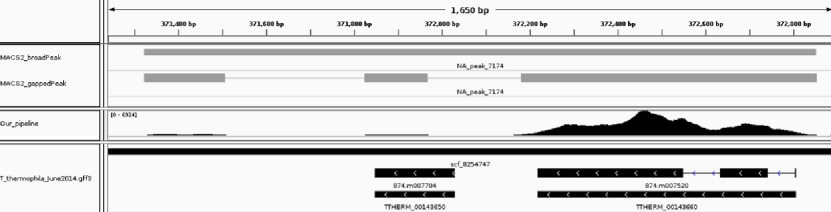
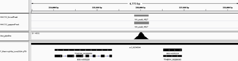
After, the determination of enriched regions we can further analyse them using a visualization tool, such as IGV. The region of interest can be copied from either the ORF or intergenic table. This localization corresponds to where the protein of interest is localizing with respect to annotated genes (see Figure 4) or an intergenic region (see Figure 5).
It is important to note that for Ibd1’s ChIP-Seq [23] data we also used MACS2 a main-stream application to call peaks [17]. The visualization option for MACS2 and RACS are similar in that both provide an specific file that can be used for this purpose. In the case of RACS, our pipeline uses .bam and .fai files which are generated within the ORF part of the pipeline (see Figure 3). Such .bam files can be opened in IGV, although the .fai (index) file will not, however both files should be present in the same directory. The required files for IGV visualization are depicted in Figure 3. In addition, the .bam files generated by RACS can be used as input for MACS2. When compared the MACS2 visualization file to the RACS .bam files using IGV (Figure 4), we observed that the RACS files provide a visual of the portion enriched. Here we observed that the IP samples are clearly enriched regions showing peaks when compared to the INPUT samples. This can be determined by noting the numbers shown in each of the IGV tracks, which represent its corresponding reads accumulation.
The output lists provided by RACS are segregated into two .csv files. The first file contain the ORF and the second the intergenic regions. Both lists contain the all reads obtained from the INPUT and IP samples. This obtained data should be filtered with the data obtained from Mock samples. We found that the output of MACS2 provides a list of peaks. MACS2 does not classify the peaks based on the localization to a gene or an intergenic region as RACS does. However, this can be addressed using BEDTools [41] after MACS2 analysis. The datasets generated by MACS2 and RACS can be found at https://www.ncbi.nlm.nih.gov/geo/query/acc.cgi?acc=GSE103318GSE103318.
3.1.3 Mock samples facilitate the analysis
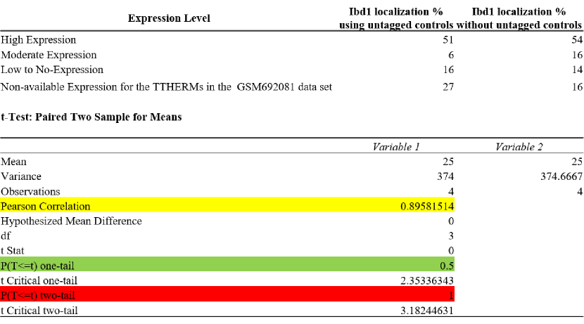
In [23] we found that the majority of genes regulated by Ibd1 were highly expressed housekeeping genes. For that analysis untagged samples were not employed, instead a cut-off based on accumulation of reads was implemented. However, since the cut-off was arbitrary there was some degree of uncertainty in regards of its astringency. To overcome this limitation and further facilitate the analysis, for this study we performed ChIP-Seq using untagged control T.thermophila cells. The addition of two mock ChIP-Seq replicas for this study (untagged T.thermophila) enhanced RACS’ ability to discriminate non specific DNA binding. In addition, the use of mock ChIP-Seq samples eliminated the uncertainty associated with using the arbitrary cut-off. This newly generated analysis will be used as a model for this case study. Between both the analysis presented in [23], and this new analysis (RACS), there are not major statistical differences regarding Ibd1 localization to genes that are highly, moderate, or low to no-expressed. The statistical analysis presented in Figure 6 shows that the hypothesis generated in [23] regarding an Ibd1 function related to transcription of highly expressed genes stands. The calculation of this result can be found in the Result tab of the ORF table (RACS/datasets/IBD1_ORF.xlsx).
3.1.4 RACS aids in the determination of the protein of interest function
By segregating the protein’s localization between genic and intergenic, the determination of its function is rapid. After analizing the Ibd1’s data with RACS, tables with the total number of reads found in each of the 26,996 ORF and 27,780 intergenic regions were generated [23].
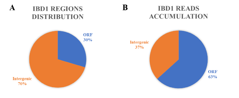
From the ORF and intergenic tables we observed that Ibd1 localizes to more individual intergenic regions than genic regions (Figure 7-A). However, the majority of reads accumulation are in the genic regions (Figure 7-B), suggesting that Ibd1 localization is within the ORF and its function maybe related to transcription regulation.
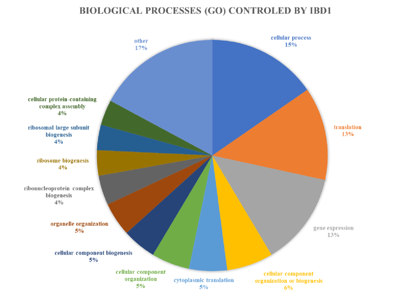
The function of Ibd1 was further inferred based on its gene-specific localization. From the ORF table (RACS/datasets/IBD1_ORF.xlsx) we observed that Ibd1 mostly localizes to genes that are highly expressed and related to housekeeping function; such as, cellular function, translation, gene expression, biogenesis, cytoplasmic translation among others (see Figure 8). The functions are based on GO annotations for biological process [42]. The calculation of this result can be found in the Gene_Ontology tab of the ORF table (RACS/datasets/IBD1_ORF.xlsx).
3.1.5 Outliers
We found a great accumulation of the following three ORFs: TTHERM_02141639, TTHERM_02641280, TTHERM_02653301; in the tagged and untagged ChIP-Seq samples. Since we found this DNA accumulated in the untagged and tagged samples we concluded that this event may be due to non-specific binding to the agarose matrix. For Ibd1, the first 2 were filter out after the subtraction step described in the “Utilities: Validation and Quality Checks” section (Sec. 2.3), and the third region seems to be controled by Ibd1.
3.2 Performance
By implementing this pipeline as described here, we obtained roughly a factor of faster in comparison to a serial and non-I/O optimized (ie. not using RAMdisk), in a equivalent hardware to the node used in the cluster. This is something we have also observed by using similar techniques (eg. RAMdisk) in other type of bio-informatics pipelines where the hierarchy of the computational scales is dominated by the I/O parts of the code. Moreover, we processed a second set of data, that was roughly 3 times larger than the original data –which would not fit in memory (GB)–, utilizing a more modern node (i7 core) with a solid-state device (SSD), we were able to furher reduce the processing time approximately by another factor of . This type of trend is typical in cases where performance is dominated by computations and I/O operations (eg. reading and writting files), for which the combination of faster processing plus faster access to the data is essential for improving the overall performance. Nevertheless, we should emphasize that even when RAMdisk or a SSD can be a solution that could in principle be thrown to similar type of problems, ie. intensively I/O demanding ones, the best approach would always be to try to mitigate and reduce as much as possible the I/O operations, as these usually represent the slowest part in any computational implementation.
4 Discussion
In this paper, we have presented a pipeline implementation utilizing open source tools. This pipeline aids in the rapid analysis of ChIP-Seq data grouping the reads accumulation from gene or intergenic regions throughout a contig based genome. The objective is to infer protein function based on its chromatin occupancy. This pipeline has been applied to Tetrahymena thermophila’s ChIP-Seq data, but its application can be extended to ChIP-Seq datasets generated in any other organisms.
We called peaks using MACS2, the output of this application was efficient; however, did not elucidate whether the protein of interest localizes to a genic or an intergenic region. Different to MACS2 that calls all peaks regardless of their position in a genic or intergenic region, RACS was designed with that very same goal in mind, hence the diferentiation in the modules that are offered in our pipeline. We should also notice that other tools such as BEDTools, can be used to perform this task in combination with MACS2.
Without the need of any additional “external” software, RACS calls reads and segregates them on a genic or intergenic regions table. Thus our pipeline is more suitable to answer biological questions regarding function. We believe that MACS2 is complementary to RACS, in that both are peaks and reads accumulation predictors. As shown in Figure 4, by obtaining a top hit from RACS this regions can be compared or assessed by MACS2 at the same time to obtained a more robust result.
It is important noting that some regions presented in the processed table have very few reads after substracting the values obtained from untagged samples . For instance, a sample that has 2 reads in the INPUT and 10 reads in the IP will return an enrichment of 5 and it may pass the filter of 1.5X enrichment. Even when there are many computational tools available for processing ChIP-Seq data, RACS is particularly suitable for contig genomes with limited annotations. Recently several ChIP-Seq studies [43, 44] have emerged for T.Thermophila. However, there is a lack of standardized computational methods for this model organism, hence it becomes difficult to reliably reach at the same conclusions when replicating the findings. Our tool is the first effort in T.Thermophila to provide a community resource for genome-wide ChIP-Seq studies, therefore it will contribute in standardizing the analyses. Other tools, such as, MACS2 and metagene using BEDTools analysis [41] complement RACS.
Last but not least, we must also note that our tool is of a broad utility and can be easily used for any other model system for ChIP-Seq analyses.
5 Conclusions
RACS is an excellent tool for genomes that are contig-based and/or have poor annotations, it permits the segregation of reads accumulation after ChIP-Seq processing. RACS is complementary to other tools, such as MACS2, as it can help to discriminate complex regions improving the overall analysis.
RACS offers an alternative tool with a different approach focused on a simple, modular and open approach. RACS offers a versatile, agile and modular pipeline that cover many of the steps needed in the process of analysing ChIP-Seq data.
The pipeline uses HPC tools, such as RAMdisk or batch processing via scheduling in cluster type environments, so that the data analysis can be done for large datasets. The scripts are reusable and generic enough that can be simply modified and utilized in other pipelines as well.
The modular approach we followed when developing RACS, also allows for future developments as this pipeline could be easily ported as a backend of a web interface, or a gateway portal, serving a larger group of researchers from different disciplines.
Declarations
Ethics approval and consent to participate
Not applicable.
Consent for publication
Not applicable.
Availability of data and materials
ChIP-Seq data used to develop this methodolgy can be found online at Gene
Expression Omnibus (GEO) http://www.ncbi.nlm.nih.gov/geo/ GSE103318 and GSE125576.
NGS and peak files produced in this study were deposited at
https://www.ncbi.nlm.nih.gov/geo/ with unique identifiers GSE103318 and GSE125576 (please use the following token: shqnagaefhilrsz).
Direct links:
http://www.ncbi.nlm.nih.gov/geo/query/acc.cgi?acc=GSE103318
and
http://www.ncbi.nlm.nih.gov/geo/query/acc.cgi?acc=GSE125576.
RACS pipeline (including a README file with instructions in how to use the scripts)
can be accessed through any of the following repositories:
Competing interests
The authors declare that they have no competing interests.
Funding
Work in the Fillingham laboratory was supported by Natural Sciences and Engineering Research Council of Canada (NSERC) Discovery Grants RGPIN-2015-06448. SciNet is funded by: the Canada Foundation for Innovation under the auspices of Compute Canada; the Government of Ontario; Ontario Research Fund—Research Excellence; and the University of Toronto.
Author’s contributions
AS defined the alignment steps using BWA and SAMtools and the reads extraction methodology and MP automated these steps by developing the scripts. AS conceived the reads extraction methodology for the intergenic regions and MP developed and automated it. AS and MP analysed the data, designed the study and wrote the manuscript. AS and SNS prepared the ChIP samples from untagged strains. JF conceived the study, coordinated and edited the manuscript. All authors read and approved the final manuscript.
Acknowledgements
We acknowledge Tanja Durbic from the Donnelly Sequencing Centre at the University of Toronto for sequencing our ChIP samples.
References
- [1] Loken, C., Gruner, D., Groer, L., Peltier, R., Bunn, N., Craig, M., Henriques, T., Dempsey, J., Yu, C.-H., Chen, J., Dursi, L.J., Chong, J., Northrup, S., Pinto, J., Knecht, N., Zon, R.V.: SciNet: Lessons Learned from Building a Power-efficient Top-20 System and Data Centre. Journal of Physics: Conference Series 256(1), 012026 (2010)
- [2] Ponce, M., Spence, E., Gruner, D., van Zon, R.: Scientific computing, high-performance computing and data science in higher education. Journal of Computational Science Education (2019). doi:10.22369/issn.2153-4136/10/1/5. 1604.05676
- [3] Venter, e.a. J. Craig: The sequence of the human genome. Science 291(5507), 1304–1351 (2001). doi:10.1126/science.1058040
- [4] The NIH HMP Working Group, Jane Peterson, et al: The nih human microbiome project. Genome Research 19(12) (2009). doi:10.1101/gr.096651.109
- [5] Wang, Zhong; Gerstein, Mark; Snyder, Michael: Rna-seq: a revolutionary tool for transcriptomics. Genetics 10(1) (2009). doi:10.1038/nrg2484
- [6] Ng, Sarah B; Turner, Emily H; Robertson, Peggy D; Flygare, Steven D; Bigham, Abigail W; et al.: Targeted capture and massively parallel sequencing of 12 human exomes. Nature 461(7261) (2009)
- [7] Schuster, S.C.: Next-generation sequencing transforms today’s biology. Nature Methods 5 (2008). doi:10.1038/nmeth1156
- [8] Loman, N., Misra, R., Dallman, T., Constantinidou, C., Gharbia, S., Wain, J., Pallen, M.: Corrigendum: Performance comparison of benchtop high-throughput sequencing platforms. Nature Biotechnology 30 (2012). doi:10.1038/nbt0612-562f
- [9] Johnson, D.S., Mortazavi, A., Myers, R.M., Wold, B.: Genome-wide mapping of in vivo protein-dna interactions. Science 316(5830), 1497–1502 (2007). doi:10.1126/science.1141319. http://science.sciencemag.org/content/316/5830/1497.full.pdf
- [10] Park, P.J.: Chip–seq: advantages and challenges of a maturing technology. Nature Reviews Genetics 10 (2009). doi:10.1038/nrg2641
- [11] Mardis, E.R.: The impact of next-generation sequencing technology on genetics. Trends in Genetics 24 (2008). doi:0.1016/j.tig.2007.12.007
- [12] Li, H., Durbin, R.: Fast and accurate short read alignment with Burrows–Wheeler transform. Bioinformatics 25(14), 1754 (2009). doi:10.1093/bioinformatics/btp324
- [13] Li, H., Handsaker, B., Wysoker, A., Fennell, T., Ruan, J., Homer, N., Marth, G., Abecasis, G., Durbin, R.: The Sequence Alignment/Map format and SAMtools. Bioinformatics 25(16), 2078 (2009). doi:10.1093/bioinformatics/btp352
- [14] R Core Team: R: A Language and Environment for Statistical Computing. R Foundation for Statistical Computing, Vienna, Austria (2016). R Foundation for Statistical Computing. https://www.R-project.org/
- [15] Cremer, T., Cremer, C.: Chromosome territories, nuclear architecture and gene regulation in mammalian cells. Nature Reviews.Genetics 2(4), 292–301 (2001). Copyright - Copyright Nature Publishing Group Apr 2001; Last updated - 2013-01-27
- [16] Schmidt, D., Wilson, M.D., Ballester, B., Schwalie, P.C., Brown, G.D., Marshall, A., Kutter, C., Watt, S., Martinez-Jimenez, C.P., Mackay, S., Talianidis, I., Flicek, P., Odom, D.T.: Five-vertebrate chip-seq reveals the evolutionary dynamics of transcription factor binding. Science 328(5981), 1036–1040 (2010). doi:10.1126/science.1186176
- [17] Zhang, Y., Liu, T., Meyer, C.A., Eeckhoute, J., Johnson, D.S., Bernstein, B.E., Nusbaum, C., Myers, R.M., Brown, M., Li, W., Liu, X.S.: Model-based analysis of chip-seq (macs). Genome Biology 9(9), 137 (2008). doi:10.1186/gb-2008-9-9-r137
- [18] Stover, N.A., Krieger, C.J., Binkley, G., Dong, Q., Fisk, D.G., Nash, R., Sethuraman, A., Weng, S., Cherry, J.M.: Tetrahymena genome database (tgd): a new genomic resource for tetrahymena thermophila research. Nucleic Acids Research 34(suppl_1), 500–503 (2006). doi:10.1093/nar/gkj054
- [19] Feng, H., Misra, V., Rubenstein, D.: Pbs: A unified priority-based scheduler. SIGMETRICS Perform. Eval. Rev. 35(1), 203–214 (2007). doi:10.1145/1269899.1254906
- [20] Steine, M., Bekooij, M., Wiggers, M.: A priority-based budget scheduler with conservative dataflow model. In: Proceedings of the 2009 12th Euromicro Conference on Digital System Design, Architectures, Methods and Tools. DSD ’09, pp. 37–44. IEEE Computer Society, Washington, DC, USA (2009). doi:10.1109/DSD.2009.148. https://doi.org/10.1109/DSD.2009.148
- [21] McLay, R., Schulz, K.W., Barth, W.L., Minyard, T.: Best practices for the deployment and management of production hpc clusters. In: State of the Practice Reports. SC ’11, pp. 9–1911. ACM, New York, NY, USA (2011). doi:10.1145/2063348.2063360. http://doi.acm.org/10.1145/2063348.2063360
- [22] Yoo, A.B., Jette, M.A., Grondona, M.: Slurm: Simple linux utility for resource management. In: Feitelson, D., Rudolph, L., Schwiegelshohn, U. (eds.) Job Scheduling Strategies for Parallel Processing, pp. 44–60. Springer, Berlin, Heidelberg (2003)
- [23] Saettone, A., Garg, J., Lambert, J.-P., Nabeel-Shah, S., Ponce, M., Burtch, A., Thuppu Mudalige, C., Gingras, A.-C., Pearlman, R.E., Fillingham, J.: The bromodomain-containing protein ibd1 links multiple chromatin-related protein complexes to highly expressed genes in tetrahymena thermophila. Epigenetics & Chromatin 11(1), 10 (2018). doi:10.1186/s13072-018-0180-6
- [24] Robinson, J.T., Thorvaldsdóttir, H., Winckler, W., Guttman, M., Lander, E.S., Getz, G., Mesirov, J.P.: Integrative Genomics Viewer. Nature Biotechnology 29(1), 24–26 (2011)
- [25] Ponce et al.: Deploying a Top-100 Supercomputer for Large Parallel Workloads: the Niagara Supercomputer. in prep. (2019)
- [26] Tarasov, A., Vilella, A.J., Cuppen, E., Nijman, I.J., Prins, P.: Sambamba: fast processing of ngs alignment formats. Bioinformatics 31(12), 2032–2034 (2015). doi:10.1093/bioinformatics/btv098
- [27] Peterson, D.S., Gao, Y., Asokan, K., Gaertig, J.: The circumsporozoite protein of plasmodium falciparum is expressed and localized to the cell surface in the free-living ciliate tetrahymena thermophila. Molecular and Biochemical Parasitology 122(2), 119–126 (2002). doi:10.1016/S0166-6851(02)00079-8
- [28] Linder, J.U., Engel, P., Reimer, A., Krüger, T., Plattner, H., Schultz, A., Schultz, J.E.: Guanylyl cyclases with the topology of mammalian adenylyl cyclases and an n-terminal p-type atpase-like domain in paramecium, tetrahymena and plasmodium. The EMBO Journal 18(15), 4222–4232 (1999). doi:10.1093/emboj/18.15.4222. http://emboj.embopress.org/content/18/15/4222.full.pdf
- [29] Roelofs, J., Smith, J.L., Haastert, P.J.M.V.: cgmp signalling: different ways to create a pathway. Trends in Genetics 19(3), 132–134 (2003). doi:10.1016/S0168-9525(02)00044-6
- [30] Tang, Y.Z., Egerton, T.A., Kong, L., Marshall, H.G.: Morphological variation and phylogenetic analysis of the dinoflagellate gymnodinium aureolum from a tributary of chesapeake bay. Journal of Eukaryotic Microbiology 55(2), 91–99 (2008). doi:10.1111/j.1550-7408.2008.00305.x
- [31] Buchmann, K., Sigh, J., Nielsen, C.V., Dalgaard, M.: Host responses against the fish parasitizing ciliate ichthyophthirius multifiliis. Veterinary Parasitology 100(1), 105–116 (2001). doi:10.1016/S0304-4017(01)00487-3. Vaccination and Immunity against Parasites
- [32] Eisen, J.A., Coyne, R.S., Wu, M., Wu, D., Thiagarajan, M., Wortman, J.R., Badger, J.H., Ren, Q., Amedeo, P., Jones, K.M., Tallon, L.J., Delcher, A.L., Salzberg, S.L., Silva, J.C., Haas, B.J., Majoros, W.H., Farzad, M., Carlton, J.M., Smith, R.K. Jr., Garg, J., Pearlman, R.E., Karrer, K.M., Sun, L., Manning, G., Elde, N.C., Turkewitz, A.P., Asai, D.J., Wilkes, D.E., Wang, Y., Cai, H., Collins, K., Stewart, B.A., Lee, S.R., Wilamowska, K., Weinberg, Z., Ruzzo, W.L., Wloga, D., Gaertig, J., Frankel, J., Tsao, C.-C., Gorovsky, M.A., Keeling, P.J., Waller, R.F., Patron, N.J., Cherry, J.M., Stover, N.A., Krieger, C.J., del Toro, C., Ryder, H.F., Williamson, S.C., Barbeau, R.A., Hamilton, E.P., Orias, E.: Macronuclear genome sequence of the ciliate tetrahymena thermophila, a model eukaryote. PLOS Biology 4(9), 1–23 (2006). doi:10.1371/journal.pbio.0040286
- [33] Ashraf, K., Nabeel-Shah, S., Garg, J., Saettone, A., Derynck, J., Gingras, A.-C., Lambert, J.-P., Pearlman, R.E., Fillingham, J.: Proteomic analysis of histones H2A/H2B and variant Hv1 in Tetrahymena thermophila reveals an ancient network of chaperones. Molecular Biology and Evolution msz039 (2019). doi:10.1093/molbev/msz039. http://oup.prod.sis.lan/mbe/advance-article-pdf/doi/10.1093/molbev/msz039/27974900/msz039.pdf
- [34] Martindale, D.W., Allis, C.D., Bruns, P.J.: Conjugation in tetrahymena thermophila: A temporal analysis of cytological stages. Experimental Cell Research 140(1), 227–236 (1982). doi:10.1016/0014-4827(82)90172-0
- [35] Xiong, J., Lu, X., Zhou, Z., Chang, Y., Yuan, D., Tian, M., Zhou, Z., Wang, L., Fu, C., Orias, E., Miao, W.: Transcriptome analysis of the model protozoan, tetrahymena thermophila, using deep rna sequencing. PLOS ONE 7(2), 1–13 (2012). doi:10.1371/journal.pone.0030630
- [36] Bailey, T., Krajewski, P., Ladunga, I., Lefebvre, C., Li, Q., Liu, T., Madrigal, P., Taslim, C., Zhang, J.: Practical Guidelines for the Comprehensive Analysis of ChIP-seq Data. PLOS Computational Biology 9(11), 1–8 (2013). doi:10.1371/journal.pcbi.1003326
- [37] Landt, S.G., Marinov, G.K., Kundaje, A., Kheradpour, P., Pauli, F., Batzoglou, S., Bernstein, B.E., Bickel, P., Brown, J.B., Cayting, P., Chen, Y., DeSalvo, G., Epstein, C., Fisher-Aylor, K.I., Euskirchen, G., Gerstein, M., Gertz, J., Hartemink, A.J., Hoffman, M.M., Iyer, V.R., Jung, Y.L., Karmakar, S., Kellis, M., Kharchenko, P.V., Li, Q., Liu, T., Liu, X.S., Ma, L., Milosavljevic, A., Myers, R.M., Park, P.J., Pazin, M.J., Perry, M.D., Raha, D., Reddy, T.E., Rozowsky, J., Shoresh, N., Sidow, A., Slattery, M., Stamatoyannopoulos, J.A., Tolstorukov, M.Y., White, K.P., Xi, S., Farnham, P.J., Lieb, J.D., Wold, B.J., Snyder, M.: ChIP-seq guidelines and practices of the ENCODE and modENCODE consortia. Genome research 22(9), 1813–1831 (2012). doi:10.1101/gr.136184.111
- [38] Cormier, N., Kolisnik, T., Bieda, M.: Reusable, extensible, and modifiable R scripts and Kepler workflows for comprehensive single set ChIP-seq analysis. BMC Bioinformatics 17(1), 270 (2016). doi:10.1186/s12859-016-1125-3
- [39] Qin, Q., Mei, S., Wu, Q., Sun, H., Li, L., Taing, L., Chen, S., Li, F., Liu, T., Zang, C., Xu, H., Chen, Y., Meyer, C.A., Zhang, Y., Brown, M., Long, H.W., Liu, X.S.: ChiLin: a comprehensive ChIP-seq and DNase-seq quality control and analysis pipeline. BMC Bioinformatics 17(1), 404 (2016). doi:10.1186/s12859-016-1274-4
- [40] Andrews, S., et al.: FastQC: a quality control tool for high throughput sequence data (2010)
- [41] Quinlan, A.R., Hall, I.M.: BEDTools: a flexible suite of utilities for comparing genomic features. Bioinformatics 26(6), 841–842 (2010). doi:10.1093/bioinformatics/btq033. http://oup.prod.sis.lan/bioinformatics/article-pdf/26/6/841/16897802/btq033.pdf
- [42] Ashburner, M., Ball, C.A., Blake, J.A., Botstein, D., Butler, H., Cherry, J.M., Davis, A.P., Dolinski, K., Dwight, S.S., Eppig, J.T., et al.: Gene ontology: tool for the unification of biology. Nature genetics 25(1), 25 (2000)
- [43] Wang, Y., Chen, X., Sheng, Y., Liu, Y., Gao, S.: N6-adenine dna methylation is associated with the linker dna of h2a. z-containing well-positioned nucleosomes in pol ii-transcribed genes in tetrahymena. Nucleic acids research 45(20), 11594–11606 (2017)
- [44] Kataoka, K., Mochizuki, K.: Phosphorylation of an hp1-like protein regulates heterochromatin body assembly for dna elimination. Developmental cell 35(6), 775–788 (2015)
6 Figures

Appendix A Abbreviations
The following abbreviations are used in this manuscript:
| ChIP-Seq | Chromatin immunoprecipitation coupled to Next Generation Sequencing |
| NGS | Next Generation Sequencing |
| HPC | High Performance Computing |
| I/O | Input/Output |
| GPC | General Purpose Cluster |
| RACS | Rapid Analysis of ChIP-Seq data |
| MAC | Macronucleus |
| MIC | Micronucleus |
| ENCODE | Encyclopedia of DNA Elements |
| ORF | Open Region Frame |
| IGR | Intergenic Region |
| IP | Immunoprecipitated |
| FCS | Flowcell summary |
| N | Normalized |