Interference of axially-shifted Laguerre-Gaussian beams and their interaction with atoms

Abstract

Counter-propagating co-axial Laguerre-Gaussian (LG) beams are considered, not in the familiar scenario where the focal planes coincide at $z=0$, but when they are separated by a finite axial distance $d$. The simplest case is where both beams are doughnut beams which have the same linear polarisation. The total fields of this system are shown to display novel amplitude and phase distributions and are shown to give rise to a ring or a finite ring lattice composed of double rings and single central ring. When the beams have slightly different frequencies the ring lattice pattern becomes a finite set of rotating Ferris wheels and the whole pattern also moves axially between the focal planes. We show that the field of such an axially shifted pair of counter-propagating LG beams generate trapping potentials due to the dipole force which can trap two-level atoms in the components of the ring lattice. We also highlight a unique feature of this system which involves the creation of a new longitudinal optical atom trapping potential due to the scattering force which arises solely when $d\neq 0$. The results are illustrated using realistic parameters which also confirm the importance of the Gouy and curvature effects in determining the ring separation both radially and axially and gives rise to the possibility of atom tunnelling between components of the double rings.

(Authors’ post-acceptance version of the paper published in J. Opt. 21 104002, 23 Sept 2019)

(PACS Numbers: 42.50Tx; 42.50.Wk; 78.68.+m; 37.10.De; 37.10.Vz)

1 Introduction

Optical manipulation as an area of optical physics stems from the mechanical effects which laser light imposes on matter, both in the form of atoms and molecules or matter at the nanoscale. This area continues to be a subject of much interest both from a fundamental point of view and for useful applications. Research began with the pioneering work by Ashkin et al [1] who showed that light pressure applied to atoms, leads to a variety of techniques resulting, most notably, in their heating, cooling, trapping and levitation (see also [2]. The prototypical example of optical manipulation is the ‘optical tweezers’ [3] and their are recent accounts involving interferometric multi-beam and surface optical tweezers [4, 5]. However, the most celebrated manifestation of radiation pressure is in the realisation of Bose-Einstein condensation in dilute atomic systems [6].

Recently, optical manipulation received an impetus when combined with structured laser light in which optical fields can have unlimited possibilities of form in terms of spatial and phase variations [7]. Laser beams in arbitrary geometrical arrangements can be made to interfere in a specified fashion and so generate optical potential landscapes and associated forces and torques leading to atom manipulation. Ordered arrangements of interfering laser beams form the so-called optical lattices as an example of structured light [8, 9].

More recently, a new ingredient entered the arena of optical manipulation with the discovery of vortex laser light, which is light endowed with the property of orbital angular momentum (OAM)[10]. Such light beams are exemplified by the Laguerre-Gaussian (LG) beams distinguished by the two indices $l,p$ and carry OAM of magnitude $l\hbar$ per photon. The OAM property of this type of laser light is in addition to the wave polarisation, or optical spin angular momentum (SAM) property, which is intrinsic to all laser light (see [11] to [13]). In this context both atomic and nanoparticle manipulation have revealed additional effects, with the OAM features manifesting themselves as rotational motion, and new atom trapping and cooling techniques have emerged (see [14, 15, 16, 17, 18, 19, 20, 21, 22, 23, 24, 25, 26, 27, 28]). The optical spanner is one of the first applications which has been realised as the rotational form of the optical tweezers (see [15, 16, 17, 18, 19, 20, 21]).

The simplest scenario consists a single focused beam where typically the scattering force attracts the atoms towards the focal plane where the beam intensity is maximum. However an axial force in the direction of beam propagation leads to axial drifting which has been counteracted with the use of counter-propagating beams [22]. Counter-propagating LG beams with coinciding focal planes have been considered as a means of localising cold atoms in the dark regions of the total fields [29]. It has also been shown that when two vortex beams meet at their common focal plane, the interference results in a petal-like intensity pattern and such a petal pattern rotates when the two beams are slightly different in frequency, resulting in the Ferris-wheel phenomenon which was discussed first by Franke-Arnold et al [23] and later by Vickers [22]. The case of two counter-propagating Laguerre-Gaussian doughnut beams LG_l,0 and LG_-l,0 with orthogonal linear polarizations ${\mbox{\boldmath$\hat{\epsilon}$}}_{x}$ and ${\mbox{\boldmath$\hat{\epsilon}$}}_{y}$ leads to azimuthal polarization gradients and an azimuthal Sisyphus effect that can be utilized in the creation and control of a persistent current of superfluid atoms circulating in a toroidal trap (see [24, 25, 26]). In addition to the case of LG beams, the coupling of atoms to Bessel beams has been considered [27].

In this paper we consider a scenario of interference which, as far as the authors know, has not been explored before in the context of optical vortices. This simply involves the introduction of a finite spatial separation $d$ between the two focal planes of the counter-propagating LG beams, giving rise to complex intensity and phase changes. The simplest case is where both beams are doughnut beams and have the same linear polarisation $\hat{\epsilon}$. The prominent feature of the resulting intensity distribution is the overlap region of the two beams, the size of which can be controlled by changing the separation $d$ and the curvature of the beams which alter the useful length of the interference pattern. Besides the intensity, which is shown to be in the form of a finite ring lattice, new features arise due to phase variations in the phase function and its gradient. The total fields of this system are shown to display novel amplitude and phase distributions and are shown to give rise to a finite ring lattice composed of double rings and single central ring. When the beams have slightly different frequencies the interference pattern becomes a set of rotating Ferris wheels and the whole pattern also moves axially between the focal planes.

This papers is organised as follows. We firstly display the standard formalism of LG beams which is essential for the theoretical development that follows. We begin with the evaluation of the case in which the two LG beams both have low-intensity. We show that the scattering forces exhibit an additional axial component between the focal planes which is due to the axial shift and points symmetrically towards the centre of the beams. This is a new form of optical trapping of atoms based on scattering forces and arising solely due to the axial shift. Next, we deal with the general case of higher light intensities and large winding number $l$. Here, the full formalism of the interference has to be deployed, along with numerical analysis. A prominent feature of the general theory for $d\neq 0$ is the inter-mixing of the phase and amplitudes due to the shifted beams in the total fields. The full theory enables the realisations of ring Ferris wheels and axial pattern motion to be manifested between the focal planes when the shifted beams have slightly different frequencies.

The main results of this papers can be summarised as follows. (1) We identify and quantify a new trapping mechanism for two-level atoms that arises due to the scattering forces which vanishes in the more common cases with $d=0$. We feel that this result is significant, not only because of the novelty of the finding, but also because it entails an all-optical trapping mechanism that would be an alternative to other more involved trapping mechanisms such as magneto-optical trapping. (2) The one-dimensional case considered here highlights the role of the Gouy phase and curvature in that they control the spacing and number of rings in the interference pattern. We show that the phase difference controls various features including the number and spacing (both radially and axially) of the rings. (3) We also point out and quantify effects that would be of interest to experimentalists, including atom trapping by both the scattering force and the dipole force and we examine regimes for atom tunnelling between double rings in the finite lattice.

2 LG optical modes

The electric field vector distribution of a single LG mode, characterised by the integers $l$ and $p$, of frequency $\omega$ and axial wavevector $k$ travelling along the positive z-axis, can be written in cylindrical coordinates ${\bf r}=(r,\phi,z)$ as follows

$${\bf E}_{klp}(\rho,\phi,z)=U_{klp}e^{i\Theta_{klp}(\rho,\phi,z)}e^{i\omega t}{\mbox{\boldmath$\hat{\epsilon}$}},$$ (1)

where $\hat{\epsilon}$ is the wave polarisation vector, $U_{klp}(r,\phi,z)$ is the amplitude function and $\Theta_{klp}(r,\phi,z)$ is the phase function. We have for the amplitude function

$$U_{klp}(\rho,\phi,z)={\cal U}_{k00}\frac{C_{lp}}{(1+z^{2}/z_{R}^{2})^{1/2}}\left(\frac{\sqrt{2}\rho}{{w(z)}}\right)^{|l|}L^{|l|}_{p}\left(\frac{2\rho^{2}}{{w}^{2}(z)}\right)e^{-\rho^{2}/{w}^{2}(z)}.$$ (2)

Here $L^{|l|}_{p}$ is the associated Laguerre polynomial; ${\cal U}_{k00}$ is the amplitude for a corresponding plane wave of wavevector $k$; $C_{lp}$ is a constant and $w(z)$ is the beam waist at position $z$ such that $w^{2}(z)=2(z^{2}+z_{R}^{2})/kz_{R}$, where $z_{R}$ is the Rayleigh range. For the phase function we have

$$\Theta_{klp}(z)=kz+l\phi+\Theta_{Gouy}+\Theta_{curv}+i\omega t,$$ (3)

where

$$\Theta_{Gouy}=-(2p+|l|+1)\tan^{-1}(z/z_{R});\;\;\;\;\;\;\;\Theta_{curv}=\frac{k\rho^{2}z}{2(z^{2}+z_{R}^{2})}.$$ (4)

The first term in the phase function is the usual term representing plane wave propagation with axial wavevector $k$ and the second term is the azimuthal phase which gives rise to $l$ intertwined helical wavefronts and is the basis for the OLM contents of the beam. The third term is the Gouy phase and the final term enters as a phase contribution due to the variation of the beam curvature with both $\rho$ and $z$.

3 Optical forces on two-level atoms

We focus on the interaction of a two-level atom of transition frequency $\omega_{0}$ and dipole moment $\mu$ with the LG light of frequency $\omega$ and electric field as describe above. In the steady steady such an atom is subject to position- and velocity-dependent forces. A moving atom in the field of a single LG beam experiences two forces: a scattering force and a dipole force

$${\bf F}_{klp}={\bf F}^{scatt}_{klp}+{\bf F}^{dipole}_{klp},$$ (5)

where ${\bf F}^{scatt}_{klp}$ is the scattering force

$${\bf F}^{scatt}_{klp}({\bf r,v)}=\frac{\hbar\Gamma}{4}\Omega^{2}_{klp}({\bf r})\left(\frac{{\mbox{\boldmath$\nabla\!$}}\Theta_{klp}({\bf r})}{\Delta_{klp}^{2}({\bf r,v})+\Omega^{2}_{klp}({\bf r})/2+\Gamma^{2}/4}\right),$$ (6)

and ${\bf F}^{dipole}_{klp}({\bf r,v})$ is the dipole force

$${\bf F}^{dipole}_{klp}({\bf r,v})=-\frac{1}{2}\hbar\Omega_{klp}({\bf r}){\mbox{\boldmath$\nabla\!$}}\Omega_{klp}\left(\frac{\Delta_{klp}({\bf r,v})}{\Delta_{klp}^{2}({\bf r,v})+\Omega^{2}_{klp}({\bf r})/2+\Gamma^{2}/4}\right),$$ (7)

where $\Omega_{klp}$ is the Rabi frequency and $\Delta_{klp}({\bf r,v})$ is the position- and velocity-dependent detuning. We have

$$\Omega_{klp}=\left|\frac{{\mbox{\boldmath$\mu$}}\cdot{{\bf E}}_{klp}}{\hbar}\right|;\;\;\;\;\;\Delta_{klp}({\bf r,v})=\Delta_{0}-{\bf v.}{\mbox{\boldmath$\nabla\!$}}\Theta_{klp}({\bf r,v}),$$ (8)

where $\Delta_{0}=\omega-\omega_{0}$. The dipole force is derivable in terms of the gradient of the dipole potential as follows [14]

$${\bf F}^{dipole}_{klp}({\bf r,v})=-{\mbox{\boldmath$\nabla$}}V^{dipole}_{klp}({\bf r,v}),$$ (9)

where

$$V^{dipole}_{klp}({\bf r,v})=\frac{1}{2}\hbar{\Delta}_{klp}({\bf r,v})\ln{\left[1+\frac{\Omega_{klp}^{2}({\bf R})/2}{\Delta_{klp}^{2}({\bf r,v})+\Gamma_{klp}^{2}/4}\right]}.$$ (10)

Both the scattering force and dipole potential are well known when using ordinary (i.e. non-vortex) laser light in the context of atom cooling and trapping. The scattering force is a net frictional force responsible for optical molasses, and the dipole potential traps the atom in regions of extremum light intensity.

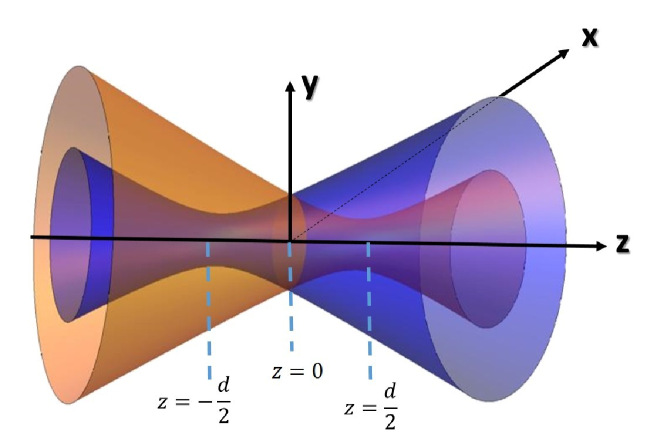
Figure 1: Schematic representation of the shifted counter-propagating LG beams where beam 1 is taken to propagate along the positive z-direction with its focal plane positioned at $z=-d/2$ while beam 2 is propagating along the negative z-direction with its focal plane at $z=+d/2$. We also assume that the two beams have the same polarisation $\hat{\epsilon}$.

4 Axially-shifted counter-propagating LG beams

The physical system involves two counter-propagating LG beams, as shown schematically in Fig. 1 where beam 1 is taken to propagate along the positive z-direction with its focal plane positioned at $z=-d/2$ while beam 2 is propagating along the negative z-direction with its focal plane at $z=+d/2$. We also assume that the two beams have the same polarisation $\hat{\epsilon}$. We consider the case where both beams have low intensity with low winding number $l$ and at near resonance. The influence of the weak light beams on a two-level atom in the region between the focal planes is the sum of individual forces arising from the two beams. The beams we are dealing with are doughnut beams for which $p=0$ and the same winding number $l$. Then the Gouy phase is negligible and we also drop the curvature phase term in this treatment. For ease of notation, we drop the mode label ${klp}$ and the superscripts defining the optical forces $scat$ and $dipole$. At near-resonance, where $Delta_{0}$ is small, the dipole force of a two-level atom is small and the scattering force dominates.

We seek to identify the first feature introduced by the shifting of the beam focal planes, so we shall consider velocity-independent i.e. static optical forces. Setting ${\bf v}=0$, there are two scattering forces on the atom arising from the two beams which we can conveniently describe using cylindrical polar coordinates ${\bf r}=({\mbox{\boldmath$\rho$}},z)$, with ${\mbox{\boldmath$\rho$}}=(\rho,\phi)$ the in-plane position vector component in polar coordinates. We have

$${\bf F}_{1}({\bf r})=\frac{\hbar\Gamma}{4}\frac{\Omega^{2}({\mbox{\boldmath$\rho$}},z+d/2)}{\Delta_{0}^{2}+\Gamma^{2}/4+\Omega^{2}({\mbox{\boldmath$\rho$}},z+d/2)/2}\left[k{\mbox{\boldmath$\hat{z}$}}+\frac{l}{\rho}{\mbox{\boldmath$\hat{\phi}$}}\right],$$ (11)

$${\bf F}_{2}({\bf r})=\frac{\hbar\Gamma}{4}\frac{\Omega^{2}({\mbox{\boldmath$\rho$}},z-d/2)}{\Delta_{0}^{2}+\Gamma^{2}/4+\Omega^{2}({\mbox{\boldmath$\rho$}},z-d/2)/2}\left[-k{\mbox{\boldmath$\hat{z}$}}+\frac{l}{\rho}{\mbox{\boldmath$\hat{\phi}$}}\right],$$ (12)

Recall that the mode labels have been suppressed for ease of notation and $\Omega$ is the Rabi frequency and $\Gamma$ is the inverse lifetime of the excited state of the two-level atom.

The total force acting on the atom is the sum

$${\bf F}({\bf r})={\bf F}_{1}({\bf r})+{\bf F}_{2}({\bf r}).$$ (13)

We are interested in the region between the focal planes as a trapping region for atoms and by symmetry we expect the total force to be the same with reference to the centre of the system, located at $z=0$. Hence we seek to explore the small $|z|$ region using Taylor expansion. We have the leading order

$${\bf F}_{1}({\bf r})\approx\frac{\hbar\Gamma}{4}\left[k{\mbox{\boldmath$\hat{z}$}}+\frac{l}{\rho}{\mbox{\boldmath$\hat{\phi}$}}\right]\left\{Q_{+}(z=0)+z\left(\frac{\partial Q_{+}}{\partial z}\right)_{z=0}\right\}.$$ (14)

where

$$Q_{+}=\frac{\Omega^{2}({\mbox{\boldmath$\rho$}},z+d/2)}{\Delta_{0}^{2}+\Gamma^{2}/4+\Omega^{2}({\mbox{\boldmath$\rho$}},z+d/2)/2}$$ (15)

A similar Taylor expansion can be carried out for ${\bf F}_{2}$ and we note that at $z=0$ we have $Q_{+}=Q_{-}$ and $\Omega^{2}_{d/2}=\Omega^{2}_{-d/2}$. Adding the contributions from ${\bf F}_{1}$ and ${\bf F}_{2}$ to leading order, we find

$${\bf F}({\bf r})=\frac{\hbar\Gamma k}{2}\left(\frac{\partial Q_{+}}{\partial z}\right)_{z=0}z{\mbox{\boldmath$\hat{z}$}}+\frac{2l}{\rho}Q_{+}(z=0){\mbox{\boldmath$\hat{\phi}$}}.$$ (16)

where

$$\left(\frac{\partial Q_{+}}{\partial z}\right)_{z}=-d\frac{(\Delta_{0}^{2}+\Gamma^{2}/4)\Omega^{2}(z=d/2)}{[\Delta_{0}^{2}+\Gamma^{2}/4+\Omega^{2}(z=d/2]^{2}}\left\{\frac{(|l|+1)(z_{R}^{2}+d^{2}/4)-2\rho^{2}z_{R}^{2}/w_{0}^{2}}{(z_{R}^{2}+d^{2}/4)^{2}}\right\}.$$ (17)

We see that the axial total force is a quasi-restoring force centred at $z=0$ and can be written as

$${\bf F}_{z}=-{\cal K}z,$$ (18)

where ${\cal K}$ is the spring ‘constant’, which here is weakly dependent on $\rho$. We have

$${\cal K}=\frac{\hbar\Gamma k}{2}d\frac{(\Delta_{0}^{2}+\Gamma^{2}/4)\Omega^{2}(z=d/2)}{[\Delta_{0}^{2}+\Gamma^{2}/4+\Omega^{2}(z=d/2]^{2}}\left\{\frac{(|l|+1)(z_{R}^{2}+d^{2}/4)-2\rho^{2}z_{R}^{2}/w_{0}^{2}}{(z_{R}^{2}+d^{2}/4)^{2}}\right\}.$$ (19)

The total axial force exhibits a quasi-harmonic trapping potential between the foci which is centred at $z=0$, where the two beams supply the same intensity with a combined single doughnut ring. This central doughnut ring is of radius $\rho_{0}$ and it is at an axial distance $d/2$ from the focal planes. We have $\rho_{0}=\sqrt{w^{2}(z=d/2)l/2}$. Substituting for $w(z=d/2)$ and noting that $w^{2}_{0}=2z_{R}/k$ we find $\rho_{0}=w_{0}\sqrt{l/2}\sqrt{1+\frac{d^{2}}{4z_{R}^{2}}}$. Note that the spring ’constant’ ${\cal K}$ depends on the radial coordinate $\rho$, as given in Eq.(19). This takes a simpler form at the radial position $\rho=\rho_{0}$, i.e. at the central doughnut ring. Substituting for $\rho=\rho_{0}$ we find that the expression between the curly brackets in Eq.(19) becomes equal to unity and we find

$${\cal K}_{0}={\cal K}(\rho_{0},z=0)=\frac{\hbar\Gamma k}{2}d\frac{(\Delta_{0}^{2}+\Gamma^{2}/4)\Omega^{2}(z=d/2)}{\left\{[\Delta_{0}^{2}+\Gamma^{2}/4+\Omega^{2}(z=d/2]^{2}(z_{R}^{2}+d^{2}/4)\right\}}.$$ (20)

This is a constant which depends on the system parameters, most notably, the separation $d$. Figure 2 displays the variations of the spring constant ${\cal K}_{0}$ with $d$ for a typical set of parameters, as stated in the caption to the figure.

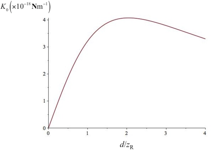
Figure 2: The variation of the spring constant ${\cal K}_{0}$ with $d$ for sodium atoms with the transition ${}^{2}S_{1/2}-^{2}P_{3/2}$ of wavelength $\lambda_{0}=589.16\;$ nm and $\Gamma=2\pi\times 10.01\;$MHz. Other parameters are as follows: $\Delta_{0}=0.5\Gamma$, $w_{0}=8\mu$m$,\Omega_{0}=\Gamma$, where $\Omega_{0}$ is the Rabi frequency corresponding to a field with an amplitude ${\cal U}_{k00}$ appearing in Eq.(2).

Since ${\cal K}_{0}$ is a constant, we may now talk about a true harmonic potential $V_{0}(z)$ associated with the axial scattering force and so write

$$V_{0}(z)=\frac{1}{2}{\cal K}_{0}z^{2},$$ (21)

so that $F_{z}(z)=-{\mbox{\boldmath$\nabla$}}V_{0}(z)$. The physical situation is now clear in that the atoms will be trapped within the axial potential well with a minimum at the plane $z=0$. The azimuthal component at $\rho_{0}$, given by ${\bf F}_{\phi}=(2l/\rho_{0})Q_{+}(z=0){\mbox{\boldmath$\hat{\phi}$}}$ of the scattering force acts to rotate the atoms by the light induced torque given by

$${\bf T}={\bf r}\times{\bf F}_{\phi}=2lQ_{+}(\rho_{0},z=0){\mbox{\boldmath$\hat{z}$}}.$$ (22)

where $Q_{+}$ is given by Eq.(15).

The above treatment is applicable in the low intensity limit and also does not take into account the situations involving focused beams with significant contributions from the Gouy phase and the curvature phase. Our next task is to explore the general case where interference is an important ingredient along with moderate focussing, so that we are still within the paraxial regime and the full LG formalism described at the outset is applicable.

5 Mixing phases and amplitude functions

We now consider the general case where the beams are sufficiently intense and the winding number $l$ is sufficiently large for the curvature effects, including the Gouy phase to come into play. With the two beams having the same polarisation $\hat{\epsilon}$, the total field is simply the sum of the field vectors.

Once again, for ease of notation we suppress the LG mode labels $klp$ and restore these when the need arises. For beams 1 and 2 we write,

$${\bf E}_{1}=U_{1}e^{i\Theta_{1}}{\mbox{\boldmath$\hat{\epsilon}$}};\;\;\;\;\;\;{\bf E}_{2}=U_{2}e^{i\Theta_{2}}{\mbox{\boldmath$\hat{\epsilon}$}},$$ (23)

where the amplitude functions $U_{1}$ and $U_{2}$ and phase function $\Theta_{1}$ and $\Theta_{2}$ are appropriate for LG beams of the forms in Eqs.(2) and (3).

Since the beam polarisations are the same we write for the total field

$${\bf E}=Ue^{i\Theta}{\mbox{\boldmath$\hat{\epsilon}$}},$$ (24)

where $U$ and $\Theta$ are the total amplitude function and the total phase function of the interfering beams. The evaluation of these functions proceeds as follows

$$Ue^{i\Theta}=\left(U_{1}e^{i\Theta_{1}}+U_{2}e^{i\Theta_{2}}\right).$$ (25)

Writing the complex exponentials on the right-hand side in terms of sine and cosine functions of $\Theta_{1}$ and $\Theta_{2}$, followed by separation of real and imaginary part we are then able to write straight forwardly for the total amplitude function

$$U=\left\{U_{1}^{2}+U_{2}^{2}+2U_{1}U_{2}\cos(\Theta_{1}-\Theta_{2})\right\}^{1/2}.$$ (26)

For the total phase function we have

$$\Theta=\tan^{-1}\left\{\frac{U_{1}\sin\Theta_{1}+U_{2}\sin\Theta_{2}}{U_{1}\cos\Theta_{1}+U_{2}\cos\Theta_{2}}\right\}.$$ (27)

Equations (26) and (27) succinctly represent the interference of any two LG beams. The total amplitude function shows interference effects residing in the cosine function involving the phase difference $\Theta_{1}-\Theta_{2}$. On the other hand the total phase involves the amplitude functions. As we show below this inter-mixing of the amplitudes and phases in the total field turns out to be the source of interesting effects in the context of LG beams.

6 Axially-shifted counter-propagating doughnut beams

Our main concern here is to explore the specific case of shifted counter-propagating LG modes and proceed to determine their intensity and phase distributions and their influence on the atoms with which they interact at near resonance. For simplicity we continue to focus on doughnut beams $LG_{l_{1},0}$ and $LG_{l_{2},0}$.

As before, we assume that the two beams have the same frequency $\omega$ and we take the focal plane of beam 1 to be situated at the point $z=-d/2$ and that of beam 2 to be situated at $z=d/2$, with the origin of coordinates situated at z=0, as shown in Fig.1. we have for the amplitude and phase of beam 1

$$U_{1}=U(z\rightarrow z-d/2);\;\;\;\;\Theta_{1}=\Theta(z\rightarrow z-d/2).$$ (28)

where $U$ and $\Theta$ are adaptable from by Eqs.(2) and (3). Similarly, the expressions appropriate for beam 2 can be written where $z\rightarrow z+d/2$.

6.1 Total phase function

In writing the phase function of beam 2 we must take into account that this beam is travelling along -z in addition to the shift of focal plane. Once the expressions for $U_{1},U_{2},\Theta_{1}$ and $\Theta_{2}$ have been determined the the total phase function follows by direct substitution in Eq.(27)

6.2 Total amplitude function and power density

The total amplitude function is given by Eq.(26) where we need to substitute for $U_{1}$ and $U_{2}$, but we also need to evaluate the phase difference. We find since the beams have the same frequency $\omega$

$$\Theta_{1}-\Theta_{2}=2kz+(l_{1}+l_{2})\phi+\Delta\Theta_{Gouy}+\Delta\Theta_{curv},$$ (29)

where

$$\Delta\Theta_{Gouy}=-(|l_{1}|+1)\tan^{-1}\left(\frac{z-d/2}{z_{R}}\right)-(|l_{2}|+1)\tan^{-1}\left(\frac{z+d/2}{z_{R}}\right).$$ (30)

For counter-propagating doughnut beams with $l_{1}=l_{2}=l$ this simplifies to

$$\Delta\Theta_{Gouy}=-(|l|+1)\tan^{-1}\left\{\frac{2zz_{R}}{z_{R}^{2}-(z^{2}+d^{2}/4)}\right\}$$ (31)

For $\Delta\Theta_{curv}$ we find

$$\Delta\Theta_{curv}=\frac{k\rho^{2}d}{2(z^{2}+z_{R}^{2})}.$$ (32)

The explicit form of the phase difference $\Theta_{1}-\Theta_{2}$ is

$$\Theta_{1}-\Theta_{2}=2kz+2l\phi-(|l|+1)\tan^{-1}\left\{\frac{2zz_{R}}{z_{R}^{2}-(z^{2}+d^{2}/4)}\right\}+\frac{k\rho^{2}d}{2(z^{2}+z_{R}^{2})}.$$ (33)

This enables the total power density distribution to be evaluated involving realistic parameters as described in the caption to Fig. 3 and 4.

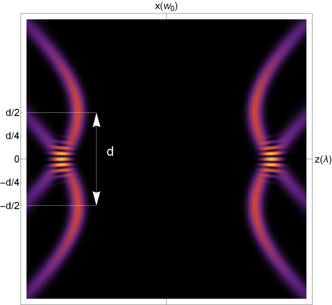
Figure 3: The intensity profile of the interference pattern of two counter-propagating doughnut LG beams. The pattern is shown projected on the $x$-$z$ plane at $y=0$ with the focal planes at $z=-d/2$ and $z=d/2$, with the centre of this cylindrically symmetric system located at $z=0$. The two sides of the interference fringes form the cross-section of the concentric rings, shown in figure 4. The parameters used here are as follows: $l_{1}=l_{2}=80$, $w_{0}=6\lambda$ and $d=24w_{0}$. These paraxial parameters are consistent with those adopted by Chu et al.[2]

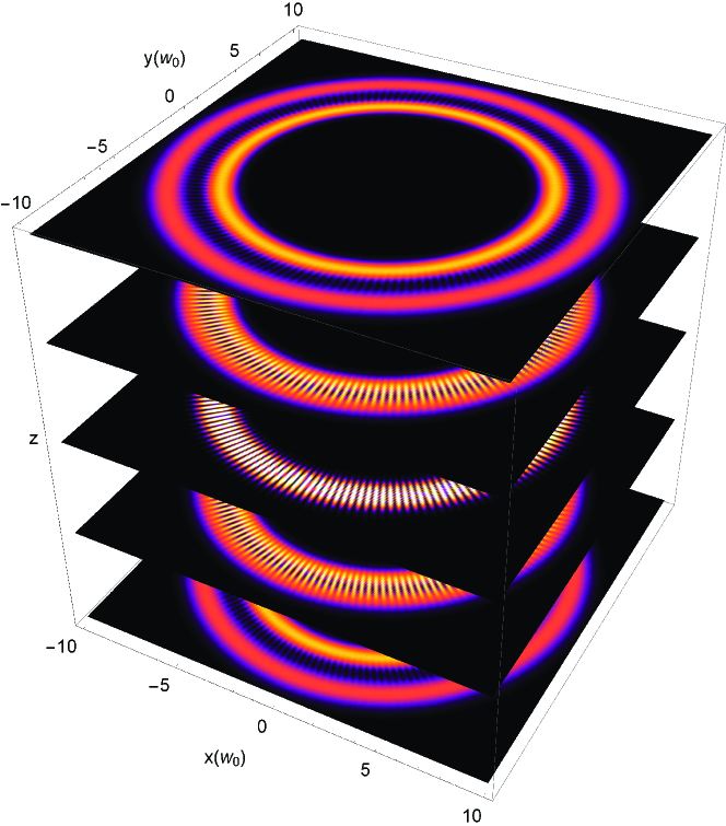
Figure 4: The interference intensity pattern projected on the $xy$ planes in the region between the focal planes. The parameters are as in Fig. 3. This figure shows a central rings at $z=0$ and double rings on either sides of this central ring. The modulation is due to the cosine of the phase difference $\cos{(\Theta_{1}-\Theta_{2})}$ entering the total amplitude function equation (26).

The superposition is seen to give rise to a standing wave in the form of a finite ring lattice of coaxial intensity rings spanning the axial region between the focal planes. The modulation in the power density pattern is governed by the cosine of the phase difference $\cos(\Theta_{1}-\Theta_{2})$ entering the total amplitude function.

6.3 Effects of frequency shift

In addition to the beams being shifted in space along the common axis, it is possible for their frequencies to differ slightly by $\Delta\omega$ in which case the total amplitude function becomes

$$U=\left\{U_{1}^{2}+U_{2}^{2}+2U_{1}U_{2}\cos(\Theta_{1}-\Theta_{2}-\Delta kz-\Delta\omega t\right\}^{1/2},$$ (34)

where $\Delta\omega=\omega_{1}-\omega_{2}$ and $\Delta k=k_{1}-k_{2}$. The $\Delta k$ term is responsible for axial beating/dephasing effects exhibited by the envelope function in the z-direction. These are typically negligible for laser beams as the dephasing length $2\pi/\Delta k$ is typically much longer than the longitudinal coherence length of the laser beam. Since the argument of the cosine function in Eq.(34)is now time-dependent leading to optical Ferris wheels and lift.

6.4 Optical Ferris wheels and lifts

The time dependence arising due to the frequency shift $\Delta\omega$ means that the interference pattern now moves with time. A given plane, for instance the symmetry plane $z=0$, can be shown to shift with time. There is azimuthal motion in every doughnut ring in the interference pattern between the focal planes which moves at an angular frequency $v_{\phi}$ given by

$$v_{\phi}=\frac{d\phi}{dt}=\frac{\Delta\omega}{2l}.$$ (35)

Thus, in the context of shifted beams this is a manifestation of the so-called optical Ferris wheel described by Franke-Arnold et al. [23]. An additional effect arising from the introduction of a frequency difference $\Delta\omega$ is a translation of the interference pattern along the $z$-axis at a speed $v_{z}$ given by

$$v_{z}=\frac{dz}{dt}\approx\frac{\Delta\omega}{2k},$$ (36)

where the approximation is necessitated by having dropped the Gouy phase and curvature phase terms in the argument of the cosine function. This is a reasonable approximation for the case of beams with large Rayleigh range $z_{R}$, and/or small winding number $l$. In the present context the motion of the interference pattern along the $z$-axis is a manifestation of the so-called lifting effect, or the conveyor belt effect.

6.5 Radial shifts in double rings

As Fig. 4 shows, the interference intensity pattern consists of a set of double doughnut rings, with a single central ring at $z=0$. On either side of this brightest ring there are rings separated by a radial distance $\delta\rho$, depending on the position $z$. We see that there is a double ring at $z=(d/2-\delta)$ where $\delta$ is the fringe separation. One of the double rings is a distance equal to $d/2-\delta$, from the focal plane of beam 1 while the second ring is a distance of $d/2+\delta$ from the focal plane of beam 2. Thus the radii of the rings are given by

$$w_{1}=w_{0}\sqrt{|l|/2}\sqrt{[1+(d/2-\delta)^{2}/z_{R}^{2}]};\;\;\;\;\;w_{2}=w_{0}\sqrt{|l|/2}\sqrt{[1+(d/2+\delta)^{2}/z_{R}^{2}]}.$$ (37)

The radial separation is the difference. We have

$$\Delta\rho=w_{0}\sqrt{|l|/2}\left(\sqrt{1+(d/2+\delta)^{2}/z_{R}^{2}}-\sqrt{1+(d/2-\delta)^{2}/z_{R}^{2}}\right).$$ (38)

For small $d$ or large $z_{R}$ this radial separation is approximately $\Delta\rho\approx w_{0}\sqrt{2|l|}(d\delta/z_{R}^{2})$. This provides the possibility of choosing the parameters in such a manner that the two component rings can be made to be very close to each other. If atoms are trapped in these rings, they can tunnel between the rings for sufficiently small radial separations. For $l$ small this could be advantageous when compared with schemes where LG beams with the same $l$, but $p=1$ are examined for atom tunnelling between ring traps. In that case, the inner ring is separated from the outer one by a radial distance of $w_{0}$, while in the current case the factor $\alpha=\sqrt{2|l|}(d\delta/z_{R}^{2})$ may be arranged to be less than unity.

7 Conclusions

The system we have considered here, namely that involving counter-propagating LG beams with axially shifted focal planes, as far as we know, has not been explored before in the context of twisted light. This requires the introduction of a spatial separation $d$ between the two focal planes of the counter-propagating LG beams, giving rise to novel intensity and phase distributions. We have concentrated on the case in which the LG beams are doughnut beams and both beams are assumed to be linearly polarized in the same direction so that when the total field is constructed as the sum of the field vectors, a total amplitude function and a total phase function can be defined and are found to be intertwined, due to spatial variations in the individual beams. The properties of the total fields can be controlled by changing the separation d and the curvature of the beams which alters the useful length of the interference pattern. In addition to the intensity distribution, which is shown to consist of a finite ring lattice, significant other properties are identified due to variations in the total phase function and its gradient. We have also shown that when the frequencies of the beams differ slightly the interference pattern becomes a set of rotating Ferris wheels which also move axially between the focal planes, identified as a conveyor belt in this context.

The summary of our main results is as follows: (1) We have identified and quantified a new trapping mechanism of two-level atoms that arises due to the scattering force, which vanishes in the more common cases in which $d=0$. We feel that this result is significant, not only because of the novelty of the finding, but also because it entails an all-optical trapping mechanism that would be an alternative to other more involved trapping mechanisms such as magneto-optical trapping. (2) The one-dimensional case considered here highlights the role of the Gouy phase and curvature in that they control the spacing and number of the rings in the interference pattern. We have emphasised the role of the phase difference $\Theta_{1}-\Theta_{2}$ in controlling various features including the number and spacing (both radially and axially) of the rings. (3) We have pointed out and quantified effects that would be of interest to experimentalists, including atom trapping by both scattering and dipole forces and have examined regions for atom tunnelling between double rings.

ORCID IDs

K Koksal https://orcid.org/0000-0001-8331-9380
Vasileios E Lembessis https://orcid.org/0000-0002-2000-7782
J Yuan https://orcid.org/0000-0001-5833-4570
M Babiker https://orcid.org/0000-0003-0659-5247

References

References

- [1] Ashkin A, Dziedzic J M, Bjorkholm J E and Chu S 1986 Observation of a single-beam gradient force optical trap for dielectric particles Optics Letters 11 288.
- [2] Chu, Steven and Bjorkholm, J. E. and Ashkin, A. and Cable, A. 1986 Experimental observation of optically trapped atoms Physical Review Letters 57 314.
- [3] Ashkin A 1970 Acceleration and trapping of particles by radiation pressure Physical Review Letters 24 156.
- [4] Mohammadnezhad, Mohammadbagher and Hassanzadeh, Abdollah 2017 Multibeam interferometric optical tweezers Journal of Nanophotonics, 11 036007.
- [5] Mohammadnezhad, Mohammadbagher and Hassanzadeh, Abdollah 2017 Evanescent field interferometric optical tweezers with rotational symmetric patterns Journal of the Optical Society of America B, 34 983.
- [6] Anderson M H, Ensher J R, Matthews M R Weiman C E and Cornell E A 1995 Observation of Bose-Einstein condensation in a dilute atomic vapour Science 269 198.
- [7] Andrews D L (ed) 2008 Structured Light and its Applications, an Introduction to Phase- structured Beams and Nanoscale Optical Forces (Burlington MA : Academic).
- [8] Jessen P S, Gerz C, Lett P D, Phillips W D, Rolston S L Spreewv R J C and Westbrook C I 1992 Observation of quantized motion of Rb atoms in an optical field Physical Review Letters 69 49.
- [9] Verkerk P, Lounis B, Salamon C, Cohen-Tannoudji C, Courtouis J Y and Grynberg G 1992 Dynamics and spatial order of cold cesium atoms in a periodic optical potential Physical Review Letters 88 3861.
- [10] Allen L, Beijersbergen R J, Spreeuw and Woerdman J P 1992. Orbital angular momentum of light and the transformation of Laguerre-Gaussian laser modes.Physical Review A 45 8185.
- [11] Torres J P and Torner L (eds) 2011 Twisted Photons: Applications of Light with Orbital Angular Momentum (Bristol : Wiley-VCH)
- [12] Andrews D L and Babiker M (eds) 2013 The Angular Momentum of Light (Cambridge : Cambridge University Press)
- [13] Barnett S M , Babiker M and Padgett M J 2017 Theme Issue: Optical orbital angular momentum Phil. Trans. R. Soc. 375, issue 2087
- [14] Babiker M, Andrews D L and Lembessis V E 2018 Atoms in complex twisted light Journal of Optics 21 013001.
- [15] He H, Friese M, Heckenburg N and Robinstein-Dulop H 1995 Direct observation of transfer of angular momentum to absorptive particle from a laser beam with a phase singularity Phys. Rev. Lett. 75 826.
- [16] Friese M E J, Nieminen T A, Heckenberg N R and Robinstein-Dunlop H 1998 Optical alignment and spinning of laser-trapped microscopic particlesNature 394 348
- [17] Clifford M A, Arlt J, Courtial J and Dholakia K 1998 High-order Laguerre-Gaussian laser modes for studies of cold atoms Opt. Comun. 156 300.
- [18] Dholakia K, M. Macdonald M and Spalding G 2002 Optical tweezers: the next generation Phys. World 15 31.
- [19] Grier D G 2003 A revolution in optical manipulation Nature 424 810.
- [20] Ladavac K and Grier D G 2004 Microoptomechanical pumps assembled and driven by holographic optical vortex arrays Opt. Express 12 1144.
- [21] Galajda P and Ormos P 2001 Complex Micromachines produced and driven by light Appl. Phys. Lett. 78 249.
- [22] Vickers J, Burch M, Vyas R and Singh S 2008 Phase and interference properties of optical vortex beams Journal of the Optical Society of America A 25 823.
- [23] Franke-Arnold S, Leach J, Padgett M J, Lembessis V E , Ellinas D, Wright A J, Girkin J M, Ohberg P and Arnold A S 2007 Optical Ferris wheel for ultra cold atoms Optics Express 15, 8619.
- [24] Anderson M F, Ryu C, Clade′ P, Natarajan V, Vaziri A, Helmerson K and Phillips W D 2006 Quantized rotation of atoms from photons with orbital angular momentum Phys. Rev. Lett. 97 170406.
- [25] Lembessis V E, Ellinas D and Babiker M 2011 Azimuthal Sisyphus effect for atoms in a toroidal all-Optical trap Phys. Rev. A 84 043422.
- [26] Lembessis V E and Babiker M 2016 Mechanical Effects on Atoms interacting with highly twisted Laguerre-Gaussian light Phys. Rev. A 94 043854.
- [27] Hayrapetyan, Armen G., Matula O, Surzhykov A , and Fritzsche S 2013 Bessel beams of two-Level atoms driven by a linearly polarized laser field European Physical Journal D: Atomic, Molecular, Optical and Plasma Physics 67 1.
- [28] Al Rsheed A, Lembessis V E, Lyras A and Aldossary O M, 2016 Rotating optical tubes for vertical transport of atoms J. Phys. B 49 125002.
- [29] Arnold A S 2012 Extending dark opticaL trapping geometries Opt. Lett. 37 2505